Sector models—A toolkit for teaching general relativity: II. Geodesics

Abstract

Sector models are tools that make it possible to teach the basic principles of the general theory of relativity without going beyond elementary mathematics. This contribution shows how sector models can be used to determine geodesics. We outline a workshop for high school and undergraduate students that addresses gravitational light deflection by means of the construction of geodesics on sector models. Geodesics close to a black hole are used by way of example. The contribution also describes a simplified calculation of sector models that students can carry out on their own. The accuracy of the geodesics constructed on sector models is discussed in comparison with numerically computed solutions. The teaching materials presented in this paper are available online for teaching purposes at www.spacetimetravel.org.

Keywords: general relativity, geodesics, black hole, gravitational light deflection, sector models

1 Introduction

To teach the basic principles of the general theory of relativity without going beyond elementary mathematics remains a challenge even a century after the completion of the theory. In view of this objective, we describe a novel approach that is focussed on geometric insight and makes do with elementary mathematics as taught in school. This approach is suitable for learners who lack the qualifications or the time required to master the mathematical tools that are needed for a standard introductory text, i.e., advanced high school students and undergraduate students, especially those in a physics minor programme or in physics teacher education. The approach can also be used as a supplement to standard textbooks (e.g., Hartle 2003) to strengthen geometric insight.

In a first paper (Zahn and Kraus 2014, in the following referred to as paper I), we have developed sector models as a new type of physical model for curved spaces and spacetimes. We have shown how they can be used to convey the notion of a space or a spacetime being curved. In paper I, sector models were first introduced for two-dimensional curved surfaces of positive or negative curvature. They were then developed for three-dimensional curved spaces and 1+1-dimensional curved spacetimes using the Schwarzschild black hole as an example.

Sector models implement the description of curved spacetimes used in the Regge calculus (Regge 1961) in the form of physical models. Figure 1 illustrates the basic principle using the surface of the earth by way of example: The surface is approximated by means of small flat elements of area. When these are laid out in the plane, one obtains a world map; this map is the sector model of the surface of the earth. Two differences to ordinary world maps stand out: The sector map is non-contiguous, since it is not possible to join all sectors simultaneously to all their neighbours. Also, the sector map is undistorted within the bounds of the discretization error, preserving both lengths and angles. It is, therefore, open to an intuitive geometric understanding. The sector model of a curved three-dimensional space is built along the same lines. The flat elements of area are replaced by blocks with euclidean geometry. In the case of a curved spacetime, the sectors are spacetime blocks with Minkowski geometry.

The general theory of relativity describes the paths of light and of free particles as geodesics of a curved spacetime. The notion of geodesics, therefore, is an important point in any introduction to general relativity. This contribution shows how sector models can be used to introduce the concept of geodesics and to determine geodesics by graphic construction. Instead of solving a system of ordinary differential equations, geodesics are constructed with pencil and ruler. The construction implements the description of geodesics in the Regge calculus (Williams and Ellis 1981) and gives quantitatively correct results (within the discretization error).

In this contribution, we outline a workshop on gravitational light deflection the way we teach it for high school and for undergraduate students (section 2). Section 3 is a discussion of the approximations involved in the construction of geodesics on sector models and a study of the accuracy that can be achieved. Conclusions and outlook follow in section 4.

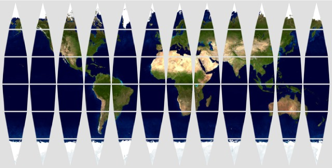
Figure 1: Sector model of the surface of the earth. Earth texture: NASA.

2 Workshop on geodesics and light deflection

The workshop starts by introducing the concept of geodesics, using curved surfaces by way of example. Geodesics are then constructed on the sector model of a black hole in order to show how gravitational light deflection arises. The black hole is used as an example because close to it relativistic effects are large and, therefore, clearly visible in the graphic constructions. As an extension to the workshop, we describe a simplified procedure for the calculation of sector models that students can use to create sector models on their own. This enables them to study the geodesics of a spacetime starting from a given metric.

2.1 Geodesics on curved surfaces

The introduction to the workshop includes the explanation that the general theory of relativity describes the paths of light and of free particles as geodesics. Depending on the background of the participants, the significance of geodesics in general relativity may just be stated or may be explained in more detail with reference to the equivalence principle (e.g., Natário 2011, chapter 5). In preparation for the determination of geodesics in the vicinity of a black hole, geodesics are first studied on curved surfaces.

The geodesic line on a curved surface is introduced as a locally straight line. Such a line keeps its direction at each point, i.e., it neither bends nor kinks. A criterion is described that permits to recognize a geodesic: One imagines that a narrow strip made of a non-elastic material is glued along its centre line onto the line that is to be investigated. If the line bends, the strip tears on the outside and buckles on the inside—this shows that the line is not a geodesic.

Figure 2: The geodesics on the sphere are the great circles.

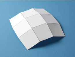
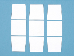
Figure 3: A spherical cap is approximated by facets (a) and represented as a sector model (b).

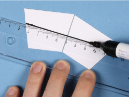
Figure 4: The construction of a geodesic on a sector model.

The sphere is used as the first example (figure 2). We consider a line that starts from the equator due north and is locally straight. It is obvious that the line is a line of longitude. The lines of longitude, and more generally all great circles, are geodesics on the sphere. Figure 2 illustrates a characteristic property of these geodesics: Two lines of longitude are parallel at the equator; towards the north pole they converge. Generally speaking, geodesics on the sphere converge when starting in parallel.

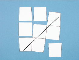
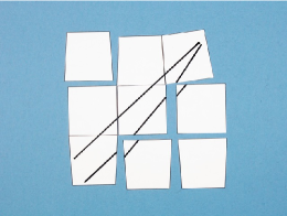
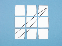
Figure 5: Geodesics on the sector model of a spherical cap. In (a) the sectors are joined along the bottom geodesic and in (b) along the top geodesic. The two geodesics are parallel in the bottom left sector and converge towards the right hand side ((b), (c)).

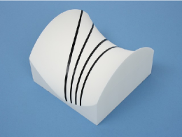
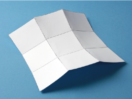
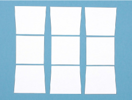
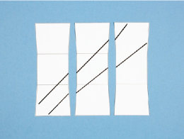
Figure 6: A saddle (a) is in part approximated by facets (b) and represented as a sector model (c); geodesics starting parallel to each other diverge ((a), (d)).

In the next step we show how this property of geodesics on the sphere can be obtained from a sector model. A spherical cap is approximated by facets (figure 3(a)), and the facets are laid out as a sector model (figure 3(b)). Now a geodesic is drawn onto the sector model. Within a sector, i.e., on a flat element of area, a geodesic is a straight line. When the line reaches the border of a sector, it is continued onto the neighbouring sector. How to do this follows from the definition of the geodesic: locally straight (figure 4). The two neighbouring sectors are joined at their common edge and the line is continued straight across the border. In this way the geodesic is continued across the sector model (figure 5(a)). A second geodesic is then added that is parallel to the first in the bottom left sector (figure 5(b)). One can see that the two geodesics starting in parallel on the lower left converge towards the right hand side (figures 5(b), (c)).

A saddle is taken as a second example. Adhesive strips glued to the surface show that geodesics starting parallel to each other diverge (figure 6(a)). The approximation of a part of the surface by facets (figure 6(b)) leads to the sector model (figure 6(c)). On the sector model, two geodesics are constructed that are parallel to each other in the lower left sector; these geodesics diverge (figure 6(d)).

The two examples show that sector models of curved surfaces can be used as tools to study the properties of geodesics on these surfaces.

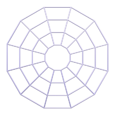
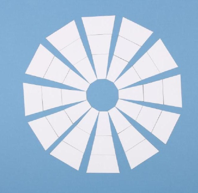
Figure 7: A thought experiment on the construction of the sector model of the black hole equatorial plane: A lattice is erected around the black hole according to the pattern shown in (a). For each cell, the lengths of the four enclosing rods are measured and from these data paper sectors are constructed true to scale. The result is the sector model of a ring around the black hole (b).

2.2 Geodesics close to a black hole

The second part of the workshop begins with the presentation of a sector model that permits to construct geodesics in the vicinity of a black hole. The sector model represents a plane of symmetry of the black hole that in the following we will call equatorial plane.

To introduce the sector model, its ”construction” is described in a thought experiment: A spaceship is sent to a black hole with the task of surveying the space around it. To this end, a lattice is erected around the black hole according to the pattern shown in figure 7(a): Rigid rods are arranged like an orb web in the equatorial plane, centred on the black hole. The whole lattice is located outside of the event horizon because no such static structure is possible in the inner region of the black hole. Measurements are taken of the lattice: Each cell is enclosed by four rods. The lengths of the rods are measured and the data sent to Earth. There, each cell, reduced in size, is represented by a sector. The complete set of sectors forms a true to scale model of a ring around the black hole (figure 7(b)). Obviously, the sectors cannot be arranged to cover a ring without leaving gaps. This indicates that the geometry of the black hole equatorial plane is different from the geometry of the plane surface on which the sectors are laid out. The equatorial plane of the black hole is part of a curved space; the flat support of the model is a plane in euclidean space. If one could place a black hole with the appropriate mass in the centre of the model, then all the flat pieces with the sizes and shapes as shown would fit without gaps. The required mass amounts to about three earth masses for the cut-out sheet that is provided online (Zahn and Kraus 2018).

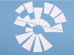
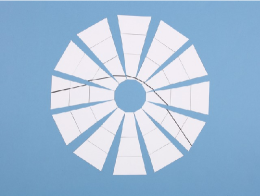
Figure 8: A geodesic on the sector model of the equatorial plane of a black hole. The line is locally straight; the direction ”far behind” the black hole differs from the direction ”far ahead”. In (a) the sectors are joined along the geodesic and in (b) they are arranged symmetrically.

Alternatively, the sector model can be introduced via the workshop on curved space described in paper I. This workshop presents a sector model of the curved three-dimensional space around a black hole (figure 5(b) in paper I). The equatorial plane of this model (in figure 5(b) of paper I: the green, nearly horizontal sides of the blocks) is identical with the sector model shown in figure 7(b).

To build the sector model shown in figure 7(b), the sectors are cut out of a sheet of paper and are glued onto cardboard with spray adhesive (use repositionable spray adhesive for repeated lifting and repositioning). The sector model is then used to study geodesics close to a black hole. First a single geodesic is drawn across the sector model. As in the case of the curved surfaces described above, this is done by joining neighbouring sectors and drawing a straight line (figure 8(a)). It can be seen that the two end sections of the line point in different directions (Fig 8(b)). Thus, for a line that passes close to a black hole while keeping its direction at each point, the direction ”far behind” the black hole differs from the direction ”far ahead”. This construction illustrates the principle underlying light deflection in a gravitational field: Light propagates on a locally straight path; when it passes a region of curved space, the direction of propagation afterwards is different from that before.

Two things must be borne in mind when assessing the significance of this construction on a sector model. First, the geodesics constructed on sector models are quantitatively correct. When the condition of a locally straight line is expressed mathematically, the result is the geodesic equation (Weinberg 1972, p. 70 ff). The graphically constructed geodesic is a solution of this equation. Since the sector model is an approximate representation of the curved space, the geodesic drawn on it is likewise an approximate solution. Using an appropriately fine subdivision, geodesics can in principle be graphically constructed with high accuracy (section 3). Secondly one must bear in mind that though the line constructed above is a geodesic, it is not a light ray. This line is a geodesic in space. But light propagates in space and time, meaning that light rays are spacetime geodesics. Nevertheless, the geodesic in space illustrates by way of close analogy the principle behind gravitational light deflection.

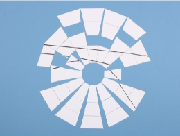
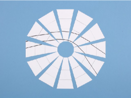
Figure 9: To the geodesic shown in figure 8, a second geodesic is added that on the far left is parallel to the first: The inner geodesic is deflected more strongly, and the two geodesics diverge. In (a) the sectors are joined along the second geodesic, in (b) they are arranged symmetrically.

Even though geodesics in space are not identical with light rays, it is instructive to use them for demonstrating properties of geodesics. One may for instance construct a second geodesic that starts close to the first and in the same direction (figure 9). The geodesic that runs closer to the black hole is deflected more strongly and the two geodesics diverge.

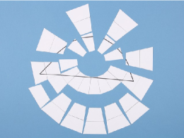
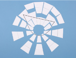
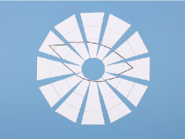
Figure 10: Two geodesics form a digon. This illustrates the formation of double images due to gravitational light deflection: Light emitted from a source reaches the observer along two different paths. In (a) and (b) the sectors are joined along the first and the second geodesic, respectively, in (c) they are arranged symmetrically.

Or one may construct two geodesics that come from the same point, pass the black hole on opposite sides, and meet again (figure 10). Thus, with geodesics it is possible to form a digon. Extrapolated to light rays, this construction shows how double images arise.

2.3 The construction of geodesics using transfer sectors

  $r_{\mathrm{S}}$

Figure 11: Worksheet for the construction of geodesics close to a black hole. The worksheet includes the sector model of the equatorial plane arranged symmetrically and with tick marks (a) and a column of transfer sectors (b). The length of the scale bar indicates the Schwarzschild radius $r_{\mathrm{S}}$ of the black hole.

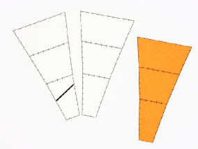
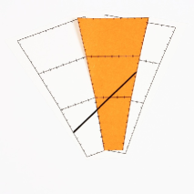
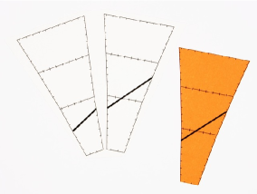
Figure 12: The construction of geodesics using transfer sectors (coloured). A geodesic is drawn up to the border of the column (a), continued across the transfer column (b), and copied from the transfer column onto the neighbouring column (c).

Figures 8, 9, and 10 show sectors that have been cut out of a sheet of paper and have been aligned along a geodesic or arranged symmetrically, as required. This procedure has the advantage that each geodesic can separately be displayed as a straight line. However, the construction of geodesics can be carried out more easily and more quickly without cutting out all the sectors. To this end, one uses the complete model in symmetric layout and with tick marks as shown in figure 11(a). A single additional column (figure 11(b)) is cut out of a sheet of paper, these are the so-called transfer sectors. The construction of a geodesic starts on the symmetric model and the line is first drawn up to the border of the column (figure 12(a)). The appropriate sector of the transfer column is then joined and the line is continued across the column of transfer sectors (figure 12(b)). The line on the transfer column is copied onto the neighbouring column of the symmetric model (figure 12(c)). This procedure is repeated up to the desired end point. In the model shown in figure 11(a), equidistant tick marks have been added at the borders to facilitate the copying of the lines. The worksheet shown in figure 11 is available online (Zahn and Kraus 2018).

2.4 The construction of sector models

A workshop can be implemented as described above, with sector models that are provided. This is the most elementary and the shortest type of workshop. But for sector models to realize their full potential as tools for studying curved spaces, the participants should calculate and construct the models on their own. This enables them to study other curved spaces in the same way, by, e.g., studying the geodesics corresponding to a given metric. Thus, setting up and solving the geodesic equation is replaced by creating the sector model and drawing the geodesics onto it.

The following section shows how one may introduce the calculation of sector models by using the sphere as an example. This procedure is then extended to the calculation of the sector model of the black hole equatorial plane.

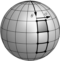
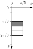
Figure 13: (a) The sphere described in polar coordinates $\theta$, $\phi$ and subdivided into elements of area of 20 degrees by 20 degrees. (b) Three elements of area in $\phi$-$\theta$ coordinate space. (c) The corresponding sectors. They make up one column of the model shown in figure 3(b). For clarity, one and the same sector is highlighted in grey in all three component images.

2.4.1 Construction of the sector model of a spherical surface.

This example serves to introduce the general procedure for the construction of sector models. The starting point is the concept of a metric as a function that takes the coordinates of two nearby points as arguments and returns their distance. This can be introduced in an elementary way by starting with curvilinear coordinates in the euclidean plane (e.g., Kraus and Zahn 2016; Hartle 2003, p. 21 f; Natário 2011, p. 35 f).

For the sector model of the sphere, the calculation is based on the metric in the usual spherical coordinates $\theta$, $\phi$ (figure 13(a)):

$$\mathrm{d}s^{2}=R^{2}\,\mathrm{d}\theta^{2}+R^{2}\sin^{2}\theta\,\mathrm{d}\phi^{2},$$ (1)

where $R$ is the radius of the sphere (for an elementary derivation that can be used in the workshop, see, e.g., Hartle 2003, p. 23 f; Natário 2011, p. 37 ff).

The creation of the sector model proceeds in three steps. In the first step the sphere is divided up into elements of area, defined by their vertices. In the example shown here, the elements of area are quadrilaterals with vertices at 20 degree ($\pi/9$) intervals in the angular coordinates $\theta$ and $\phi$, respectively (figures 13(a), (b)). In the second step the edge lengths of the quadrilaterals are computed. This is done in an approximate way in order to keep the calculation simple. For each edge, one determines the length by treating the end points as nearby points in the sense of the metric. For edges between vertices with the same longitude, one obtains the length

$$\Delta s=R\,\Delta\theta\hskip 28.45274pt(\Delta\phi=0),$$ (2)

in this example $\Delta s=R\pi/9$. For edges between two vertices of the same latitude, one finds

$$\Delta s=R\,\sin\theta\,\Delta\phi\hskip 28.45274pt(\Delta\theta=0),$$ (3)

depending on the angle $\theta$ of the circle of latitude. For the sector models shown in the figures and provided online, the distance between vertices is determined along geodesics (see paper I). The difference between the approximate and the exact edge lengths amounts to $0.13\%$ at most in this example.

In step three flat pieces of area are constructed from the edge lengths. In the present example, the elements of area on the sphere possess mirror symmetry. The flat pieces of area are constructed with the same symmetry property in the shape of symmetric trapezia (figure 13(c)).

2.4.2 Construction of the sector model of the equatorial plane of a black hole.

Figure 14: Construction of the sector model of the equatorial plane of a black hole. (a) The three elements of area of one column in $\phi$-$r$ coordinate space. (b) The corresponding sectors.

The starting point of the calculation is the metric of the equatorial plane of a black hole

$$\mathrm{d}s^{2}=\frac{1}{1-r_{\mathrm{S}}/r}\mathrm{d}r^{2}+r^{2}\mathrm{d}\phi^{2}$$ (4)

with the usual Schwarzschild coordinates $r$ and $\phi$. Here, $r_{\mathrm{S}}=2GM/c^{2}$ is the Schwarzschild radius of the black hole with mass $M$, $G$ is the gravitational constant, and $c$ the speed of light. The sector model represents an annular part of the equatorial plane, centred on the black hole. The inner rim is located at $r=1.25\,r_{\mathrm{S}}$ and the outer rim at $r=5\,r_{\mathrm{S}}$. The azimuthal angle $\phi$ has values between zero and $2\pi$.

First the ring is divided up into elements of area. For that purpose, the $\phi$-range is subdivided into twelve segments of coordinate length $\pi/6$ each. Since the metric does not depend on the coordinate $\phi$, only one of the twelve segments needs to be calculated. The $r$-range is subdivided into three segments of coordinate length $1.25\,r_{\mathrm{S}}$ each (figure 14(a)). Next, the edge lengths of the three quadrilaterals shown in figure 14(a) are calculated. Using the metric, the distance between vertices with the same value of $r$ is obtained as

$$\Delta s=r\,\Delta\phi\hskip 28.45274pt(\Delta r=0).$$ (5)

When calculating the distance of vertices with the same $\phi$-coordinate, the first term of the metric comes into play. Its metric coefficient $1\big{/}(1-r_{\mathrm{S}}/r)$ depends on $r$ and, therefore, varies along the edge. Here we make another approximation and use the metric coefficient at the mean $r$-coordinate $r_{\mathrm{m}}$ of the edge:

$$\Delta s=\sqrt{\frac{1}{(1-r_{\mathrm{S}}/r_{\mathrm{m}})}}\,\Delta r\hskip 28.45274pt(\Delta\phi=0),$$ (6)

where $r_{\mathrm{m}}=(r_{1}+r_{2})/2$ with the coordinates $r_{1}$ and $r_{2}$ of the associated vertices. The sector models shown in the figures and provided online are constructed with edge lengths that are computed numerically for geodesics joining the vertices. The difference between the approximate and the exact edge lengths is largest for the innermost radial edge and there amounts to 5.4%.

Step three is the construction of the quadrilaterals. The subdivision of the ring by radial cuts creates elements of area that possess mirror symmetry (figure 7(a)). In accordance with this symmetry, the sectors are constructed as symmetric trapezia. Figure 14 shows the three sectors of a column together with the corresponding three rectangles in $\phi-r$ coordinate space. The complete sector model with twelve columns is shown in figure 11.

2.5 Geodesics vs. curvature

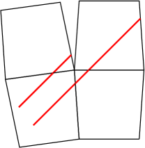
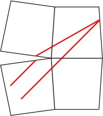
Figure 15: Two geodesics start in parallel (a), pass a vertex on opposite sides, and are then inclined towards each other by the deficit angle (b).

When the workshop described above is combined with the workshop on curvature described in paper I (section 2), it is possible to address the connection between the curvature of a surface and its geodesics. In paper I, the sphere and the saddle are introduced as prototypes of surfaces with positive and negative curvature, respectively. The deficit angle at a vertex of the sector model is shown to be a criterion for curvature: Positive curvature is indicated by a positive deficit angle and vice versa.

Using sector models, one can show that the paths of neighbouring geodesics also provide a criterion for determining curvature. Figure 15 shows neighbouring geodesics near a single vertex with positive deficit angle. Two geodesics that are parallel ahead of the vertex and pass the vertex on opposite sides (figure 15(a)) converge behind it (figure 15(b)). By construction, the angle between the two directions behind the vertex is the deficit angle.

Thus, geodesics starting in parallel indicate positive curvature if they converge. Conversely, they indicate negative curvature if they diverge. Two examples for this criterion are provided in section 2.1 in the form of geodesics on the sphere (figure 5(c)) and on the saddle (figure 6(d)). Applied to the equatorial plane of a black hole where initially parallel geodesics diverge (figure 9), one concludes that the curvature is negative.

The argument given above is an illustration of the equation of geodesic deviation

$$(\nabla_{\bf u}\nabla_{\bf u}{\bf D})^{i}=-R^{i}{}_{jkl}u^{j}D^{k}u^{l}$$ (7)

for two geodesics $x^{i}(\lambda)$ and $x^{i}(\lambda)+D^{i}(\lambda)$ with $u^{i}=dx^{i}/d\lambda$ and the Riemann curvature tensor $R^{i}{}_{jkl}$. In the sector model, the components of the Riemann curvature tensor are represented by the deficit angles (paper I, section 3) and figure 15 illustrates their impact on the change in distance between neighbouring geodesics.

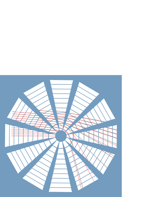
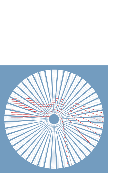
Figure 16: Geodesics constructed on sector models (red lines) in comparison with numerical solutions of the geodesic equation (black lines). (a) Sector model with the resolution used in the workshop. (b) Sector model with four times the resolution in each coordinate.

3 The accuracy of geodesics on sector models

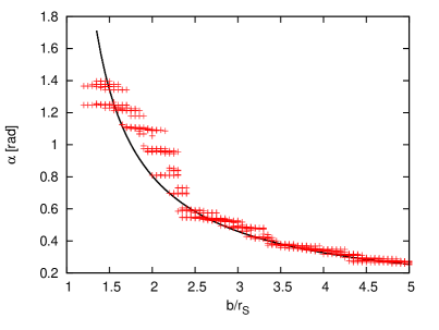
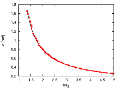
Figure 17: Relation between the angle of deflection $\alpha$ and the impact parameter $b$ of a geodesic, determined by constructing geodesics on a sector model (symbols) and by integrating the geodesic equation (line). (a) Sector model with the resolution used in the workshop. (b) Sector model with four times the resolution in each coordinate.

In the Regge calculus, geodesics are described as straight lines in the flat sectors (Williams and Ellis 1981, 1984, Brewin 1993). On the sector models, this description is implemented by graphic construction. Thus, the geodesics constructed in this way are in principle quantitatively correct. Their accuracy, however, depends on the resolution of the sector model. For use in the workshops, the resolution is deliberately chosen to be coarse, in order for the models to be easy to handle. In this section, we study the accuracy of the graphic method by comparing its results with numerically computed geodesics. Two sector models of the equatorial plane of a black hole are used in the comparison. Both cover the region between $r=1.25\,r_{\mathrm{S}}$ and $r=13.75\,r_{\mathrm{S}}$. The first one has the resolution used in the workshop ($\Delta r=1.25\,r_{\mathrm{S}}$, $\Delta\phi=\pi/6$), it consists of 10 rings of 12 sectors each (figure 16(a)). The second one has four times this resolution in each coordinate ($\Delta r=0.3125\,r_{\mathrm{S}}$, $\Delta\phi=\pi/24$), thus it consists of 40 rings of 48 sectors each (figure 16(b)). Figure 16 shows the geodesics obtained in the Regge calculus in comparison with the numerical solutions of the geodesic equation. For this comparison, the paths computed from the geodesic equation are plotted onto the sector models. The mapping of Schwarzschild coordinates onto sector points is carried out by interpolation (Hormann 2005). For a quantitative comparison, the angle of deflection as a function of the impact parameter was determined on the same two sector models and compared with the values obtained by integration (figure 17). On the sector models, ten geodesics were constructed for each value of the impact parameter. They are rotated in $\phi$-direction with respect to each other and thus have different locations with respect to the sector boundaries. For the coarser resolution, the agreement is good if the deflection is small, otherwise the deviation may be significant (figures 16(a), 17(a)). For the higher resolution sector model, the agreement is generally good (figures 16(b), 17(b)). For qualitative considerations, the accuracy on the sector model used in the workshop is satisfactory.

4 Conclusions and outlook

4.1 Summary and pedagogical comments

We have shown how sector models can be used as tools to determine geodesics. On the one hand this provides geometric insight and on the other hand it is a possibility to determine geodesics graphically. The concept of a geodesic as a locally straight line is illustrated by implementing this definition directly on a sector model using pencil and ruler (section 2.1). The graphic construction of geodesics shows that their direction after crossing a region of curved space differs from the direction they had before (section 2.2), thus showing clearly how gravitational light deflection arises. Since the graphically constructed geodesics represent solutions of the geodesic equation, one obtains quantitatively correct results. Due to the rather coarse resolution of the sector models used in the workshop, the accuracy of these geodesics is not high. From a pedagogical point of view, though, a coarse resolution is an advantage. The deficit angles are then large enough to allow the illustration of the effects of curvature by considering a single vertex. This provides a clear picture of the connection between curvature and the run of neighbouring geodesics (section 2.5). In this paper we consider spatial geodesics only. An extension to geodesics in spacetime is described in the sequel to this contribution (Kraus and Zahn 2018).

The workshop on geodesics and gravitational light deflection outlined in this contribution has been developed in several cycles of testing and revision (Kraus and Zahn 2005, Zahn and Kraus 2010, 2013, Kraus and Zahn 2016). It was mainly tested with classes grades 10 to 13 (age 16 to 19 years) and with pre-service teachers.

There are different possible uses for the material presented above, depending on the teaching goals and on the time available. If the goal is to provide a short and direct approach to the phenomenon of gravitational light deflection, e.g. in an astronomy class, then the workshop can be held as described in sections 2.1 to 2.3 with the sector models provided as worksheets. No previous knowledge of the concept of metric is required; the graphic construction is easily carried out and conveys an appropriate understanding of light paths as geodesics. In a course that aims at introducing the basic concepts of general relativity, one can let the participants compute the sector models of the sphere and of the black hole equatorial plane. The participants then acquire the necessary skills for studying the geometry of a surface when they are given the metric. Answers are here obtained graphically that in a standard university course would be found by calculations. Since sector models and the graphic construction of geodesics directly correspond to the mathematical description by means of the metric and the geodesic equation, this material can also be used as a supplement to a standard course in order to strengthen geometric insight.

4.2 Comparison with other graphic approaches

In comparison with other graphic representations of geodesics, constructions on sector models stand out by the fact that they clearly show geodesics to be locally straight as well as by their straightforward construction.

Explanations of optical phenomena due to gravitational light deflection, e.g. double images, typically use drawings that depict light rays as curved lines. In this context, light rays are described as ”bent”. These drawings and explanations do not express the fact that light paths are geodesics, i.e. (locally) straight lines, and may thereby encourage misconceptions. The construction of geodesics on sector models clearly shows that there is no contradiction between the line being locally straight and the occurrence of light deflection (figure 8). The construction can also relate geodesics to light rays being drawn as curved lines: On a world map, the surface of the earth is projected onto the plane and the geodesics of the sphere appear as curved lines. These are distortions due to the projection. Analogously, in a projection that maps the sector model of figure 8 onto a plane circular ring, there will be distortions and the geodesics in the equatorial plane of the black hole will appear curved.

A commonly used visualization shows geodesics on the embedding surface of the equatorial plane of a star or a black hole in order to illustrate the deflection of light (d’Inverno 1992, p. 209). This is equivalent to the geodesics constructed in section 2.2. When the sectors of the model shown there are joined at the common edges, one obtains a faceted surface that is an approximation of the embedding surface. The same caveat applies to the geodesics on the embedding surface as to the geodesics on the sector model: The subspace is purely spatial so that gravitational light deflection is illustrated by way of analogy with spacelike geodesics. Experience shows that the concept of an embedding surface is a difficult one for the audience at which this workshop is targeted and that the embedding surface is quite likely to be misinterpreted as the geometric shape of the black hole (Zahn and Kraus 2010). With respect to embedding surfaces, sector models have the advantage that their calculation is elementary, especially with the simplified method of section 2.4. Also, sector models are easily built as physical paper models and are readily duplicated, so that all participants of a workshop can carry out the construction of geodesics on models of their own.

A description of geodesics that is related to the representation on sector models is diSessa’s construction on so-called wedge maps (diSessa 1981). To create a wedge map, the symmetry plane of a spherically symmetric spacetime is divided up into strips by a number of radial cuts; the strips (the wedges) are regarded as flat segments. On the wedges, geodesics are determined numerically as in the Regge calculus. Thus, the construction of geodesics on the wedge map follows the same prescription that is used here for sector models. The numerical method, however, is more involved than the graphic construction used here, concerning both the mathematical description and the requirement of programming skills.

4.3 Outlook

In paper I, three fundamental questions were raised that should be answered by an introduction to general relativity: What is a curved spacetime? How does matter move in a curved spacetime? How is the distribution of matter linked to the curvature of the spacetime? The concept of curved spaces and spacetimes was discussed in paper I. To address the second question, the present part II describes geodesics in space and its sequel describes geodesics in spacetime (Kraus and Zahn 2018). The relation between curvature and the distribution of matter will be treated in a fourth part of this series.

References

- (1)
- Brewin (1993) Brewin L 1993 Particle paths in a Schwarzschild spacetime via the Regge calculus Class. Quantum Grav. 10 1803–23
- d’Inverno (1992) d’Inverno R 1992 Introducing Einstein’s Relativity (Oxford: Clarendon Press)
- diSessa (1981) diSessa A 1981 An elementary formalism for general relativity Am. J. Phys. 49 (5) 401–11
- Hartle (2003) Hartle J 2003 Gravity (San Francisco: Addison Wesley)
- Hormann (2005) Hormann K 2005 Barycentric Coordinates for Arbitrary Polygons in the Plane, Technical Report No. 5, Institute of Computer Science, Clausthal University of Technology, Germany
- Kraus and Zahn (2005) Kraus U and Zahn C 2005 Wir basteln ein Schwarzes Loch – Unterrichtsmaterialien zur Allgemeinen Relativitätstheorie Praxis der Naturwissenschaften Physik, Didaktik der Relativitätstheorien 4/54 38–43
-
Kraus and Zahn (2016)
Kraus U and Zahn C 2016
Teaching gravitational light deflection:
A short path from the metric to the geodesic
www.spacetimetravel.org/aur16
English translation of: Lichtablenkung für die Schule: Von der Metrik zur Geodäte Astronomie und Raumfahrt im Unterricht 53 (3-4/2016) 43–9 - Kraus and Zahn (2018) Kraus U and Zahn C 2018 Sector models—A toolkit for teaching general relativity: III. Spacetime geodesics, submitted
- Natário (2011) Natário J 2011 General Relativity Without Calculus (Springer)
- Regge (1961) Regge T 1961 General relativity without coordinates Il Nuovo Cimento 19 558–71
- Weinberg (1972) Weinberg S 1972 Gravitation and Cosmology (Wiley)
- Williams and Ellis (1981) Williams R M and Ellis G F R 1981 Regge Calculus and Observations. I. Formalism and Applications to Radial Motion and Circular Orbits Gen. Rel. Grav. 13 (4) 361–95
- Williams and Ellis (1984) Williams R M and Ellis G F R 1984 Regge Calculus and Observations. II. Further Applications Gen. Rel. Grav. 16 (11) 1003–21
- Zahn and Kraus (2010) Zahn C and Kraus U 2010 Workshops zur Allgemeinen Relativitätstheorie im Schülerlabor „Raumzeitwerkstatt“ an der Universität Hildesheim PhyDid B DD 09.03
- Zahn and Kraus (2013) Zahn C and Kraus U 2013 Bewegung im Gravitationsfeld in der Allgemeinen Relativitätstheorie – ein neuer Zugang auf Schulniveau PhyDid B DD 17.13
-
Zahn and Kraus (2014)
Zahn C and Kraus U 2014