A comparison of eigenvalue condition numbers for matrix polynomials

Abstract

In this paper, we consider the different eigenvalue condition numbers for matrix polynomials used in the literature and we compare them. One of these condition numbers is a generalization of the Wilkinson condition number for the standard eigenvalue problem. This number has the disadvantage of only being defined for finite eigenvalues. In order to give a unified approach to all the eigenvalues of a matrix polynomial, both finite and infinite, two (homogeneous) condition numbers have been defined in the literature. In their definition, very different approaches are used. One of the main goals of this note is to show that, when the matrix polynomial has a moderate degree, both homogeneous numbers are essentially the same and one of them provides a geometric interpretation of the other. We also show how the homogeneous condition numbers compare with the “Wilkinson-like” eigenvalue condition number and how they extend this condition number to zero and infinite eigenvalues.

1 Introduction

Let $\mathbb{C}$ denote the field of complex numbers. A square matrix polynomial of grade $k$ can be expressed (in its non-homogeneous form) as

$$P(\lambda)=\sum_{i=0}^{k}\lambda^{i}B_{i},\quad B_{i}\in\mathbb{C}^{n\times n},$$ (1)

where the matrix coefficients, including $B_{k}$, are allowed to be the zero matrix. In particular, when $B_{k}\neq 0$, we say that $P(\lambda)$ has degree $k$. Throughout the paper, the grade of every matrix polynomial $P(\lambda)$ will be assumed to be its degree unless it is specified otherwise.

The (non-homogeneous) polynomial eigenvalue problem (PEP) associated with a regular matrix polynomial $P(\lambda)$, (that is, $det(P(\lambda))\neq 0$) consists of finding scalars $\lambda_{0}\in\mathbb{C}$ and nonzero vectors $x,y\in\mathbb{C}^{n}$ satisfying

$$P(\lambda_{0})x=0\ \text{and}\ y^{*}P(\lambda_{0})=0.$$

The vectors $x$ and $y$ are called, respectively, a right and a left eigenvector of $P(\lambda)$ corresponding to the eigenvalue $\lambda_{0}$. In addition, $P(\lambda)$ may have infinite eigenvalues. We say that $P(\lambda)$ has an infinite eigenvalue if 0 is an eigenvalue of the reversal of $P(\lambda)$, where the reversal of a matrix polynomial $P(\lambda)$ of grade $k$ is defined as

$$rev(P(\lambda)):=\lambda^{k}P(1/\lambda)\,.$$ (2)

The numerical solution of the PEP has received considerable attention from many research groups in the last two decades and, as a consequence, several condition numbers for simple eigenvalues of a matrix polynomial $P(\lambda)$ have been defined in the literature to determine the sensitivity of these eigenvalues to perturbations in the coefficients of $P(\lambda)$ [2, 3, 8]. One of these condition numbers is a natural generalization of the Wilkinson condition number for the standard eigenproblem (see Definition 1). A disadvantage of this eigenvalue condition number is that it is not defined for infinite eigenvalues. Then, in order to study the conditioning of all the eigenvalues of a matrix polynomial, other condition numbers are considered in the literature. These condition numbers assume that the matrix polynomial is expressed in homogeneous form, that is,

$$P(\alpha,\beta)=\sum_{i=0}^{k}\alpha^{i}\beta^{k-i}B_{i}.$$ (3)

If $P(\alpha,\beta)$ is regular, we can consider the corresponding homogeneous PEP that consists in finding pairs of scalars $(\alpha_{0},\beta_{0})\neq(0,0)$ and nonzero vectors $x,y\in\mathbb{C}^{n}$ such that

$$P(\alpha_{0},\beta_{0})x=0\quad\ \text{and}\ \quad y^{*}P(\alpha_{0},\beta_{0})=0.$$ (4)

We note that the pairs $(\alpha_{0},\beta_{0})$ satisfying (4) are those for which $det(P(\alpha_{0},\beta_{0}))=0$ holds. Notice that $(\alpha_{0},\beta_{0})$ satisfies $det(P(\alpha_{0},\beta_{0}))=0$ if and only if $det(P(c\alpha_{0},c\beta_{0}))=0$ for any nonzero complex number $c$. Therefore, it is natural to define an eigenvalue of $P(\alpha,\beta)$ as any line in $\mathbb{C}^{2}$ passing through the origin consisting of solutions of $det(P(\alpha,\beta))=0$. For simplicity, we denote such a line, i.e., an eigenvalue of $P(\alpha,\beta)$, as $(\alpha_{0},\beta_{0})$ and by $[\alpha_{0},\beta_{0}]\neq(0,0)$ a specific representative of this eigenvalue. The vectors $x,y$ in (4) are called, respectively, a right and a left eigenvector of $P(\alpha,\beta)$ corresponding to the eigenvalue $(\alpha_{0},\beta_{0})$. For $\beta\neq 0$, we can define $\lambda=\alpha/\beta$ and find a relationship between the homogeneous and the non-homogeneous expressions of a matrix polynomial $P$ of degree $k$ as follows:

$$P(\alpha,\beta)=\beta^{k}P(\lambda).$$

We note also that, if $(y,\lambda_{0},x)$ is a solution of the non-homogeneous PEP, i.e., an eigentriple of the non-homogeneous PEP, then $(y,(\alpha_{0},\beta_{0}),x)$ is a solution of the corresponding homogeneous PEP, for any ${[\alpha_{0},\beta_{0}]\neq(0,0)}$ such that $\lambda_{0}=\alpha_{0}/\beta_{0}$, including $\lambda_{0}=\infty$ for $\beta_{0}=0$.

Two homogeneous eigenvalue condition numbers (well defined for all the eigenvalues of $P(\alpha,\beta)$, finite and infinite) have been presented in the literature. One of them is a natural generalization of the condition number defined by Stewart and Sun in [7, Chapter VI, Section 2.1] for the eigenvalues of a pencil. This condition number is defined in terms of the chordal distance between two lines in $\mathbb{C}^{2}$ (see Definition 12).

The other homogeneous eigenvalue condition number is defined as the norm of a differential map [2, 3]. The definition of this condition number is very involved and less intuitive than the definition of the other condition numbers that we consider in this paper. For an explicit formula for this condition number, see Theorem 6.

In this paper we address the following natural questions:

• how are the two homogeneous eigenvalue condition numbers related? Are they equivalent?

• if $\lambda_{0}$ is a finite nonzero eigenvalue of a matrix polynomial $P(\lambda)$ and $(\alpha_{0},\beta_{0})$ is the associated eigenvalue of $P(\alpha,\beta)$ (that is, $\lambda_{0}=\alpha_{0}/\beta_{0}$), how are the (non-homogeneous) absolute and relative eigenvalue condition numbers of $\lambda_{0}$ and the (homogeneous) condition numbers of $(\alpha_{0},\beta_{0})$ related? Are these two types of condition numbers equivalent in the sense that $\lambda_{0}$ is ill-conditioned if and only if $(\alpha_{0},\beta_{0})$ is ill-conditioned?

Partial answers to these questions are scattered in the literature written in an implicit way so that they seem to be unnoticed by most researchers in Linear Algebra. Our goal is to present a complete and explicit answer to these questions. More precisely, we provide an exact relationship between the two homogeneous eigenvalue condition numbers and we use this relationship to prove that they are equivalent. Also, we obtain exact relationships between each of the non-homogeneous (relative and absolute) and the homogeneous eigenvalue condition numbers. From these relationships we prove that the non-homogeneous condition numbers are always larger than the homogeneous condition numbers. This means that non-homogenous eigenvalues $\lambda_{0}$ are always more sensitive to perturbations than the corresponding homogeneous ones $(\alpha_{0},\beta_{0})$, which is natural since $\lambda_{0}=\alpha_{0}/\beta_{0}$. Moreover, we will see that non-homogeneous eigenvalues with large or small moduli have much larger non-homogeneous than homogeneous condition numbers. Thus, in these cases, $(\alpha_{0},\beta_{0})$ can be very well-conditioned and $\lambda_{0}$ very ill-conditioned. In the context of this discussion, it is important to bear in mind that in most applications of PEPs the quantities of interest are the non-homogeneous eigenvalues, and not the homogeneous ones.

The paper is organized as follows: Section 2 includes the definitions and expressions of the different condition numbers that are used in this work. In section 3, we establish relationships between the condition numbers introduced in section 2, and in section 4 we present a geometric interpretation of these relationships. Section 4 also includes a study of the computability of small and large eigenvalues. Finally, some conclusions are discussed in section 5.

2 Eigenvalue condition numbers of matrix polynomials

In this section we recall three eigenvalue condition numbers used in the literature and discuss some of the advantages and disadvantages of each of them. Before recalling their definition, we present some notation that will be used throughout the paper.

Let $a$ and $b$ be two integers. We define

$$a:b=\left\{\begin{array}[]{cc}a,a+1,a+2,\ldots,b,&\textrm{if $a\leq b$,}\\ \emptyset,&\textrm{if $a>b$.}\end{array}\right.$$

For any matrix $A$, $\|A\|_{2}$ denotes its spectral or 2-norm, i.e., its largest singular value [7]. For any vector $x$, $\|x\|_{2}$ denotes its standard Euclidean norm, i.e., $\|x\|_{2}=(x^{*}x)^{1/2}$, where the operator $()^{*}$ stands for the conjugate-transpose of $x$.

2.1 Non-homogeneous eigenvalue condition numbers

Next we recall the definition of two versions (absolute and relative) of a normwise eigenvalue condition number introduced in [8].

Definition 1.

Let $\lambda_{0}$ be a simple, finite eigenvalue of a regular matrix polynomial $P(\lambda)=\sum_{i=0}^{k}\lambda^{i}B_{i}$ of grade $k$ and let $x$ be a right eigenvector of $P(\lambda)$ associated with $\lambda_{0}$. We define the normwise absolute condition number $\kappa_{a}(\lambda_{0},P)$ of $\lambda_{0}$ by

$$\kappa_{a}(\lambda_{0},P):=\lim_{\epsilon\to 0}\sup\bigg{\{}\frac{|\Delta\lambda_{0}|}{\epsilon}:[P(\lambda_{0}+\Delta\lambda_{0})+\Delta P (\lambda_{0}+\Delta\lambda_{0})](x+\Delta x)=0,$$

$$\|\Delta B_{i}\|_{2}\leq\epsilon\;\omega_{i},i=0:k\bigg{\}},$$

where $\Delta P(\lambda)=\sum_{i=0}^{k}\lambda^{i}\Delta B_{i}$ and $\omega_{i}$, $i=0:k$, are nonnegative weights that allow flexibility in how the perturbations of $P(\lambda)$ are measured.

For $\lambda_{0}\neq 0$, we define the normwise relative condition number $\kappa_{r}(\lambda_{0},P)$ of $\lambda_{0}$ by

$$\kappa_{r}(\lambda_{0},P):=\lim_{\epsilon\to 0}\sup\bigg{\{}\frac{|\Delta\lambda_{0}|}{\epsilon|\lambda_{0}|}:[P(\lambda_{0}+\Delta\lambda_{0})+\Delta P (\lambda_{0}+\Delta\lambda_{0})](x+\Delta x)=0,$$

$$\|\Delta B_{i}\|_{2}\leq\epsilon\;\omega_{i},i=0:k\bigg{\}}.$$

We will refer to $\kappa_{a}(\lambda_{0},P)$ and $\kappa_{r}(\lambda_{0},P)$, respectively, as the absolute and relative non-homogeneous eigenvalue condition numbers. Note that the absolute non-homogeneous condition number is not defined for infinite eigenvalues while the relative condition number is not defined for zero or infinite eigenvalues.

Remark 2.

In the definitions of $\kappa_{a}(\lambda_{0},P)$ and $\kappa_{r}(\lambda_{0},P)$, the weights $\omega_{i}$ can be chosen in different ways. The most common ways are: 1) $\omega_{i}=\|B_{i}\|_{2}$ (relative coefficient-wise perturbations); 2) $\omega_{i}=\max\limits_{i=0:k}\{\|B_{i}\|_{2}\}$ (relative perturbations with respect to the norm of $P(\lambda)$); 3) $\omega_{i}=1$ (absolute perturbations).

An explicit formula for each of the non-homogeneous eigenvalue condition numbers presented above was obtained by Tisseur in [8].

Theorem 3.

Let $P(\lambda)$ be a regular matrix polynomial of grade $k$. Let $\lambda_{0}$ be a simple, finite eigenvalue of $P(\lambda)$ and let $x$ and $y$ be, respectively, a right and a left eigenvector of $P(\lambda)$ associated with $\lambda_{0}$. Then,

$$\kappa_{a}(\lambda_{0},P)=\frac{(\sum_{i=0}^{k}|\lambda_{0}|^{i}\omega_{i})\|y\|_{2}\|x\|_{2}}{|y^{*}P^{\prime}(\lambda_{0})x|},$$

where $P^{\prime}(\lambda)$ denotes the derivative of $P(\lambda)$ with respect to $\lambda$. For $\lambda_{0}\neq 0$,

$$\kappa_{r}(\lambda_{0},P)=\frac{(\sum_{i=0}^{k}|\lambda_{0}|^{i}\omega_{i})\|y\|_{2}\|x\|_{2}}{|\lambda_{0}||y^{*}P^{\prime}(\lambda_{0})x|}.$$

The following technical result will be useful for the comparison of the non-homogeneous condition numbers introduced above and the homogeneous condition numbers that we introduce in the next subsection. We will use the concept of reversal of a matrix polynomial defined in (2).

Lemma 4.

Let $P(\lambda)=\sum_{i=0}^{k}\lambda^{i}B_{i}$ be a regular matrix polynomial. Let $\lambda_{0}$ be a simple, nonzero, finite eigenvalue of $P(\lambda)$. Then,

$$\kappa_{a}\left(\frac{1}{\lambda_{0}},revP\right)=\frac{\kappa_{r}(\lambda_{0},P)}{|\lambda_{0}|}\quad\textrm{and}\quad\kappa_{r}\left(\frac{1}{\lambda_{0}},revP\right)=\kappa_{r}(\lambda_{0},P).$$

Proof.

We only prove the first claim. The second claim follows immediately from the first.

Let $x$ and $y$ be, respectively, a right and a left eigenvector of $P(\lambda)$ associated with $\lambda_{0}$. It is easy to see that these vectors are also a right and a left eigenvector of $revP$ associated with $\frac{1}{\lambda_{0}}$. Notice that

$$\kappa_{a}\left(\frac{1}{\lambda_{0}},revP\right) =\frac{(\sum_{i=0}^{k}\left|\frac{1}{\lambda_{0}}\right|^{k-i}\omega_{i})\|x\|_{2}\|y\|_{2}}{|y^{*}(revP)^{\prime}(\frac{1}{\lambda_{0}})x|}$$

$$=\frac{(\sum_{i=0}^{k}\left|{\lambda_{0}}\right|^{i}\omega_{i})\|x\|_{2}\|y\|_{2}}{|\lambda_{0}|^{k}|y^{*}(revP)^{\prime}(\frac{1}{\lambda_{0}})x|}=\frac{(\sum_{i=0}^{k}\left|{\lambda_{0}}\right|^{i}\omega_{i})\|x\|_{2}\|y\|_{2}}{|\lambda_{0}|^{2}|y^{*}\lambda_{0}^{k-2}(revP)^{\prime}(\frac{1}{\lambda_{0}})x|}$$

$$=\frac{(\sum_{i=0}^{k}\left|{\lambda_{0}}\right|^{i}\omega_{i})\|x\|_{2}\|y\|_{2}}{|\lambda_{0}|^{2}|y^{*}P^{\prime}(\lambda_{0})x|}=\frac{\kappa_{r}(\lambda_{0},P)}{|\lambda_{0}|},$$

where the fourth equality follows from the facts that $revP(\lambda)=\lambda^{k}P(\frac{1}{\lambda})$ and $P(\lambda_{0})x=0$, and the first and fifth equalities follow from Theorem 3. Thus, the claim follows.

∎

2.2 Homogeneous eigenvalue condition numbers

As pointed out in the last subsection, neither of the non-homogeneous condition numbers is defined for infinite eigenvalues. Thus, these type of eigenvalues require a special treatment in the non-homogeneous setting. In this section we introduce two condition numbers that allow a unified approach to all eigenvalues, finite and infinite. These condition numbers require the matrix polynomial to be expressed in homogeneous form (see (3)). This is the reason why we refer to them as homogeneous eigenvalue condition numbers.

Remark 5.

We recall that $(\alpha_{0},\beta_{0})\neq(0,0)$ is an eigenvalue of $P(\alpha,\beta)$ if and only if $\lambda_{0}:=\alpha_{0}/\beta_{0}$ is an eigenvalue of $P(\lambda)$, where $\lambda_{0}=\infty$ if $\beta_{0}=0$.

Each of the condition numbers presented in this subsection has been defined in the literature with a different approach. One of them is due to Stewart and Sun [7], who define the eigenvalue condition number in terms of the chordal distance between the exact and the perturbed eigenvalues. The other approach is due to Dedieu and Tisseur [2, 3] and makes use of the Implicit Function Theorem to construct a differential operator whose norm is defined to be an eigenvalue condition number. This idea was inspired by Shub and Smale’s work [6]. These two condition numbers do not have a specific name in the literature. We will refer to them as the Stewart-Sun condition number and the Dedieu-Tisseur condition number, respectively.

2.2.1 Dedieu-Tisseur condition number

The homogeneous eigenvalue condition number that we present in this section has been often used in recent literature on matrix polynomials as an alternative to the non-homogeneous Wilkinson-like condition number. See, for instance, [4, 5]. We do not include its explicit definition because it is much more involved than Definition 1. For the interested reader, the definition can be found in [3]. The next theorem provides an explicit formula for this condition number.

Theorem 6.

[3, Theorem 4.2] Let $(\alpha_{0},\beta_{0})$ be a simple eigenvalue of the regular matrix polynomial $P(\alpha,\beta)=\sum_{i=0}^{k}\alpha^{i}\beta^{k-i}B_{i}$, and let $y$ and $x$ be, respectively, a left and a right eigenvector of $P(\alpha,\beta)$ associated with $(\alpha_{0},\beta_{0})$. Then, the Dedieu-Tisseur condition number of $(\alpha_{0},\beta_{0})$ is given by

$$\kappa_{h}((\alpha_{0},\beta_{0}),P)=\left(\sum_{i=0}^{k}|\alpha_{0}|^{2i}|\beta_{0}|^{2(k-i)}\omega_{i}^{2}\right)^{1/2}\frac{\|y\|_{2}\|x\|_{2}}{|y^{*}(\overline{\beta_{0}}D_{\alpha}P(\alpha_{0},\beta_{0})-\overline{\alpha_{0}}D_{\beta}P(\alpha_{0},\beta_{0}))x|},$$ (5)

where $D_{a}\equiv\frac{\partial}{\partial a},$ that is, the partial derivative with respect to $a$ and $\omega_{i}$, $i=0:k$ are nonnegative weights that define how the perturbations of the coefficients $B_{i}$ are measured.

It is important to note that the expression for this eigenvalue condition number does not depend on the choice of representative for the eigenvalue $(\alpha_{0},\beta_{0})$.

2.2.2 Stewart-Sun condition number

Here we introduce another homogeneous eigenvalue condition number. Its definition is easy to convey and to interpret from a geometrical point of view.

We recall that every eigenvalue of a homogeneous matrix polynomial can be seen as a line in $\mathbb{C}^{2}$ passing through the origin. The condition number that we present here uses the “chordal distance” between lines in $\mathbb{C}^{2}$ to measure the distance between an eigenvalue and a perturbed eigenvalue. This distance is defined on the projective space $\mathbb{P}_{1}(\mathbb{C})$.

Before introducing the chordal distance, we recall the definition of angle between two lines.

Definition 7.

Let $x$ and $y$ be two nonzero vectors in $\mathbb{C}^{2}$ and let $\langle x\rangle$ and $\langle y\rangle$ denote the lines passing through zero in the direction of $x$ and $y$, respectively. We define the angle between the two lines $\langle x\rangle$ and $\langle y\rangle$ by

$$\theta(\langle x\rangle,\langle y\rangle):=arccos\frac{|\langle x,y\rangle|}{\|x\|_{2}\|y\|_{2}},\quad 0\leq\theta(\langle x\rangle,\langle y\rangle)\leq\pi/2,$$

where $\langle x,y\rangle$ denotes the standard Hermitian inner product, i.e., $\langle x,y\rangle=y^{*}x$.

Remark 8.

We note that $cos\;\theta(\langle x\rangle,\langle y\rangle)$ can be seen as the ratio between the length of the orthogonal projection (with respect to the standard inner product in $\mathbb{C}^{2}$) of the vector $x$ onto $y$ to the length of the vector $x$ itself, that is,

$$cos\;\theta(\langle x\rangle,\langle y\rangle)=\frac{\|proj_{y}x\|_{2}}{\|x\|_{2}},$$

since

$$proj_{y}x=\frac{\langle x,y\rangle y}{\|y\|_{2}^{2}}\quad\textrm{and}\quad\frac{\|proj_{y}x\|_{2}}{\|x\|_{2}}=\frac{|\langle x,y\rangle|}{\|x\|_{2}\|y\|_{2}}.$$

We also have

$$sin\;\theta(\langle x\rangle,\langle y\rangle)=\frac{\|x-proj_{y}x\|_{2}}{\|x\|_{2}}.$$

The definition of chordal distance is given next.

Definition 9.

[7, Chapter VI, Definition 1.20] Let $x$ and $y$ be two nonzero vectors in $\mathbb{C}^{2}$ and let $\langle x\rangle$ and $\langle y\rangle$ denote the lines passing through zero in the direction of $x$ and $y$, respectively. The chordal distance between $\langle x\rangle$ and $\langle y\rangle$ is given by

$$\chi(\langle x\rangle,\langle y\rangle):=sin(\theta(\langle x\rangle,\langle y\rangle)).$$

Notice that $\chi(\langle x\rangle,\langle y\rangle)\leq\theta(\langle x\rangle,\langle y\rangle).$ Moreover, the chordal distance and the angle are identical asymptotically, that is, when $\theta(\langle x\rangle,\langle y\rangle)$ approaches $0$.

The chordal distance between two lines $\langle x\rangle$ and $\langle y\rangle$ in $\mathbb{C}^{2}$ can also be expressed in terms of the coordinates of the vectors $x$ and $y$ in the canonical basis for $\mathbb{C}^{2}$. Note that this expression does not depend on the representatives $x$ and $y$ of the lines.

Lemma 10.

[7, page 283] If $\langle\alpha,\beta\rangle$ and $\langle\gamma,\delta\rangle$ are two lines in $\mathbb{C}^{2}$, then

$$\chi(\langle\alpha,\beta\rangle,\langle\gamma,\delta\rangle)=\frac{|\alpha\delta-\beta\gamma|}{\sqrt{|\alpha|^{2}+|\beta|^{2}}\sqrt{|\gamma|^{2}+|\delta|^{2}}}.$$

Remark 11.

Notice that $0\leq\chi(\langle\alpha,\beta\rangle,\langle\gamma,\delta\rangle)\leq 1$ for all lines $\langle\alpha,\beta\rangle,\langle\gamma,\delta\rangle$ in $\mathbb{C}^{2}$. Since the line $\langle 1,0\rangle$ is identified with the eigenvalue $\infty$ in PEPs, we see that the chordal distance allows us to measure the distance from $\infty$ to any other eigenvalue very easily. Moreover, such distance is never larger than one.

Next we introduce the homogeneous eigenvalue condition number in which the change in the eigenvalue is measured using the chordal distance and that we baptize as the Stewart-Sun eigenvalue condition number. This condition number was implicitly introduced for matrix pencils in [7, page 294], although an explicit definition is not given in [7]. See also [1, page 40] for an explicit definition of this condition number for matrix polynomials.

Note that in Definition 12 below, $(\alpha_{0},+\Delta\alpha_{0},\beta_{0}+\Delta\beta_{0})$ is the unique simple eigenvalue of $(P+\Delta P)(\alpha,\beta)$ that approaches $(\alpha_{0},\beta_{0})$ when $\Delta P$ approaches zero.

Definition 12.

Let $(\alpha_{0},\beta_{0})$ be a simple eigenvalue of a regular matrix polynomial $P(\alpha,\beta)=\sum_{i=0}^{k}\alpha^{i}\beta^{k-i}B_{i}$ of grade $k$ and let $x$ be a right eigenvector of $P(\alpha,\beta)$ associated with $(\alpha_{0},\beta_{0})$. We define

$$\kappa_{\theta}((\alpha_{0},\beta_{0}),P):=\lim_{\epsilon\to 0}\sup\bigg{\{}\frac{\chi((\alpha_{0},\beta_{0}),(\alpha_{0}+\Delta\alpha_{0},\beta_{0}+\Delta\beta_{0}))}{\epsilon}:$$

$$[P(\alpha_{0}+\Delta\alpha_{0},\beta_{0}+\Delta\beta_{0})+\Delta P(\alpha_{0}+\Delta\alpha_{0},\beta_{0}+\Delta\beta_{0})](x+\Delta x)=0,$$

$$\|\Delta B_{i}\|_{2}\leq\epsilon\omega_{i},i=0:k\bigg{\}},$$

where $\Delta P(\alpha,\beta)=\sum_{i=0}^{k}\alpha^{i}\beta^{k-i}\Delta B_{i}$ and $\omega_{i}$, $i=0:k$, are nonnegative weights that allow flexibility in how the perturbations of $P(\alpha,\beta)$ are measured.

As far as we know, no explicit formula for the Stewart-Sun condition number is available in the literature. We provide such an expression next.

Theorem 13.

Let $(\alpha_{0},\beta_{0})\neq(0,0)$ be a simple eigenvalue of $P(\alpha,\beta)=\sum_{i=0}^{k}\alpha^{i}\allowbreak\beta^{k-i}B_{i}$, and let $x$ and $y$ be, respectively, a right and a left eigenvector of $P(\alpha,\beta)$ associated with $(\alpha_{0},\beta_{0})$. Then,

$$\kappa_{\theta}((\alpha_{0},\beta_{0}),P)=\left(\sum_{i=0}^{k}|\alpha_{0}|^{i}|\beta_{0}|^{k-i}\omega_{i}\right)\frac{\|y\|_{2}\|x\|_{2}}{|y^{*}(\overline{\beta_{0}}D_{\alpha}P(\alpha_{0},\beta_{0})-\overline{\alpha_{0}}D_{\beta}P(\alpha_{0},\beta_{0}))x|},$$ (6)

where $D_{a}\equiv\frac{\partial}{\partial a},$ that is, the partial derivative with respect to $a$.

Proof.

Let $(P+\Delta P)(\alpha,\beta)$ be a small enough perturbation of $P(\alpha,\beta)$. Then, $(P+\Delta P)(\alpha,\beta)$ has a unique simple eigenvalue $(\tilde{\alpha_{0}},\tilde{\beta_{0}})$, with associated eigenvector $x+\Delta x$, that approaches $(\alpha_{0},\beta_{0})$ when $\Delta P(\alpha,\beta)$ approaches zero. Since $\{[\alpha_{0},\beta_{0}],[-\overline{\beta_{0}},\overline{\alpha_{0}}]\}$ is an orthogonal basis for $\mathbb{C}^{2}$ (with respect to the standard inner product), we can choose a representative for $(\tilde{\alpha_{0}},\tilde{\beta_{0}})$ of the form

$$[\alpha_{0},\beta_{0}]+[\Delta\alpha_{0},\Delta\beta_{0}],$$

where $\langle[\alpha_{0},\beta_{0}],[\Delta\alpha_{0},\Delta\beta_{0}]\rangle=0$ for any given representative $[\alpha_{0},\beta_{0}]$ of $(\alpha_{0},\beta_{0})$. This implies that there exists a scalar $\mathfrak{h}$ such that

$$[\Delta\alpha_{0},\Delta\beta_{0}]=\mathfrak{h}[-\overline{\beta_{0}},\overline{\alpha_{0}}].$$ (7)

Expanding for these representatives the left hand side of the constraint

$$[P(\alpha_{0}+\Delta\alpha_{0},\beta_{0}+\Delta\beta_{0})+\Delta P(\alpha_{0}+\Delta\alpha_{0},\beta_{0}+\Delta\beta_{0})](x+\Delta x)=0$$

in the definition of $\kappa_{\theta}((\alpha_{0},\beta_{0}),P)$ and keeping only the first order terms, we get

$$[D_{\alpha}P(\alpha_{0},\beta_{0})\Delta\alpha_{0}+D_{\beta}P(\alpha_{0},\beta_{0})\Delta\beta_{0}]x+P(\alpha_{0},\beta_{0})\Delta x+\Delta P(\alpha_{0},\beta_{0})x=O(\epsilon^{2}).$$

If we multiply the previous equation by $y^{*}$ on the left, taking into account that $y$ is a left eigenvector of $P(\alpha,\beta)$ associated with $(\alpha_{0},\beta_{0})$, we get

$$y^{*}[D_{\alpha}P(\alpha_{0},\beta_{0})\Delta\alpha_{0}+D_{\beta}P(\alpha_{0},\beta_{0})\Delta\beta_{0}]x+y^{*}\Delta P(\alpha_{0},\beta_{0})x=O(\epsilon^{2}).$$ (8)

Using (7), (8) becomes

$$y^{*}[D_{\alpha}P(\alpha_{0},\beta_{0})\mathfrak{h}\overline{\beta_{0}}-D_{\beta}P(\alpha_{0},\beta_{0})\mathfrak{h}\overline{\alpha_{0}}]x-y^{*}\Delta P(\alpha_{0},\beta_{0})x=O(\epsilon^{2}).$$

Since $(\alpha_{0},\beta_{0})\neq 0$ is a simple eigenvalue, by [3, Theorem 3.3],

$$y^{*}[D_{\alpha}P(\alpha_{0},\beta_{0})\overline{\beta_{0}}-D_{\beta}P(\alpha_{0},\beta_{0})\overline{\alpha_{0}}]x\neq 0.$$

Therefore,

$$\mathfrak{h}=\frac{y^{*}\Delta P(\alpha_{0},\beta_{0})x}{y^{*}[\overline{\beta_{0}}D_{\alpha}P(\alpha_{0},\beta_{0})-\overline{\alpha_{0}}D_{\beta}P(\alpha_{0},\beta_{0})]x}+O(\epsilon^{2}).$$ (9)

On the other hand,

$$\frac{\chi((\alpha_{0},\beta_{0}),(\alpha_{0}+\Delta\alpha_{0},\beta_{0}+\Delta\beta_{0}))}{\epsilon} =\frac{|\alpha_{0}\Delta\beta_{0}-\beta_{0}\Delta\alpha_{0}|}{\epsilon\sqrt{|\alpha_{0}|^{2}+|\beta_{0}|^{2}}\sqrt{|\alpha_{0}+\Delta\alpha_{0}|^{2}+|\beta_{0}+\Delta\beta_{0}|^{2}}}$$

$$=\frac{|\mathfrak{h}|}{\epsilon}\frac{\sqrt{|\alpha_{0}|^{2}+|\beta_{0}|^{2}}}{\sqrt{|\alpha_{0}+\Delta\alpha_{0}|^{2}+|\beta_{0}+\Delta\beta_{0}|^{2}}}.$$ (10)

Since, by (9),

$$\frac{|\mathfrak{h}|}{\epsilon}\leq\left(\sum_{i=0}^{k}|\alpha_{0}|^{i}|\beta_{0}|^{k-i}\omega_{i}\right)\frac{\|y\|_{2}\|x\|_{2}}{|y^{*}(\overline{\beta_{0}}D_{\alpha}P(\alpha_{0},\beta_{0})-\overline{\alpha_{0}}D_{\beta}P(\alpha_{0},\beta_{0}))x|}+O(\epsilon)$$ (11)

and $\Delta\alpha_{0}$ and $\Delta\beta_{0}$ approach zero as $\epsilon\to 0$, from (2.2.2) and (11) we get

$$\kappa_{\theta}((\alpha_{0},\beta_{0}),P)\leq\left(\sum_{i=0}^{k}|\alpha_{0}|^{i}|\beta_{0}|^{k-i}\omega_{i}\right)\frac{\|y\|_{2}\|x\|_{2}}{|y^{*}(\overline{\beta_{0}}D_{\alpha}P(\alpha_{0},\beta_{0})-\overline{\alpha_{0}}D_{\beta}P(\alpha_{0},\beta_{0}))x|}.$$

Now we need to show that this upper bound on the Stewart-Sun condition number can be attained. Let

$$\Delta B_{i}=sgn(\overline{\alpha_{0}}^{i})sgn(\overline{\beta_{0}}^{k-i})\epsilon\omega_{i}\frac{yx^{*}}{\|x\|_{2}\|y\|_{2}},\quad i=0:k,$$

where $sgn(z)=\frac{z}{|z|}$ if $z\neq 0$ and $sgn(0)=0$. Note that, with this definition of $\Delta B_{i}$, we have

$$\|\Delta B_{i}\|_{2}=\epsilon\omega_{i},\ i=0:k,\quad\text{and}\quad|y^{*}\Delta P(\alpha_{0},\beta_{0})x|=\epsilon\left(\sum_{i=0}^{k}|\alpha_{0}|^{i}|\beta_{0}|^{k-i}\omega_{i}\right)\|x\|_{2}\|y\|_{2}.$$

Thus, the inequality in (11) becomes an equality and the result follows. ∎

3 Comparisons of eigenvalue condition numbers of matrix polynomials

In this section we provide first a comparison between the Dedieu-Tisseur and Stewart-Sun homogeneous condition numbers and, as a consequence, we prove that these condition numbers are equivalent up to a moderate constant depending only on the degree of the polynomial. Then we compare the Stewart-Sun condition number with the non-homogeneous condition number in both its absolute and relative version; as a result, we see that these condition numbers can be very different in certain situations. A simple geometric interpretation of these differences is given in Section 4. In the literature some comparisons can be found, as we will point out, but they provide inequalities among the condition numbers while our expressions are equalities.

3.1 Comparison of the Dedieu-Tisseur and Stewart-Sun condition numbers

As mentioned earlier, the Dedieu-Tisseur and the Stewart-Sun homogeneous condition numbers are defined following a very different approach. So it is a natural question to determine how they are related. We start with a result known in the literature.

Theorem 14.

[2, Section 7][1, Corollary 2.6] Let $(\alpha_{0},\beta_{0})\neq(0,0)$ be a simple eigenvalue of a regular matrix polynomial $P(\alpha,\beta)=\sum_{i=0}^{k}\alpha^{i}\beta^{k-i}B_{i}$ of grade $k$. Assuming that the same weights $\omega_{i}$ are considered for both condition numbers, we have

$$\kappa_{\theta}((\alpha_{0},\beta_{0}),P)\leq C\kappa_{h}((\alpha_{0},\beta_{0}),P),$$

for some constant $C$.

To provide an exact relationship between the Dedieu-Tisseur and the Stewart-Sun homogeneous condition numbers, we simply use the explicit formulas given for them in Theorems 6 and 13, respectively.

Theorem 15.

Let $(\alpha_{0},\beta_{0})\neq(0,0)$ be a simple eigenvalue of $P(\alpha,\beta)=\sum_{i=0}^{k}\alpha^{i}\allowbreak\beta^{k-i}B_{i}$. Then,

$$\kappa_{h}((\alpha_{0},\beta_{0}),P)=\frac{\left(\sum_{i=0}^{k}|\alpha_{0}|^{2i}|\beta_{0}|^{2(k-i)}\omega_{i}^{2}\right)^{1/2}}{\sum_{i=0}^{k}|\alpha_{0}|^{i}|\beta_{0}|^{k-i}\omega_{i}}\ \kappa_{\theta}((\alpha_{0},\beta_{0}),P).$$

The following result is an immediate consequence of Theorem 15 and shows that, for moderate $k$, both homogeneous condition numbers are essentially the same.

Corollary 16.

Let $(\alpha_{0},\beta_{0})\neq(0,0)$ be a simple eigenvalue of $P(\alpha,\beta)=\sum_{i=0}^{k}\alpha^{i}\beta^{k-i}B_{i}$. Then,

$$\frac{1}{\sqrt{k+1}}\leq\frac{\kappa_{h}((\alpha_{0},\beta_{0}),P)}{\kappa_{\theta}((\alpha_{0},\beta_{0}),P)}\leq 1.$$

Proof.

Let $v:=[|\beta_{0}|^{k}\omega_{0},|\alpha_{0}||\beta_{0}|^{k-1}\omega_{1},\ldots,|\alpha_{0}|^{k}\omega_{k}]^{T}\in\mathbb{R}^{k+1}$. From Theorem 15, we have

$$\frac{\kappa_{h}((\alpha_{0},\beta_{0}),P)}{\kappa_{\theta}((\alpha_{0},\beta_{0}),P)}=\frac{\|v\|_{2}}{\|v\|_{1}},$$

where $\|.\|_{1}$ denotes the vector 1-norm [7]. The result follows taking into account the fact that $1/\sqrt{k+1}\leq\|v\|_{2}/\|v\|_{1}\leq 1.$ ∎

Since the Dedieu-Tisseur and the Stewart-Sun condition numbers are equivalent and the definition of the Stewart-Sun condition number is much simpler and intuitive, we do not see any advantage in using the Dedieu-Tisseur condition number. Therefore, in the next subsection, we focus on comparing the Stewart-Sun condition number with the non-homogeneous condition numbers. The corresponding comparisons with the Dedieu-Tisseur condition number follow immediately from Theorem 15 and Corollary 16.

3.2 Comparison of the homogeneous and non-homogeneous eigenvalue condition numbers

As we mentioned in Section 2, the main drawback of the non-homogeneous condition numbers is that they do not allow a unified treatment of all the eigenvalues of a matrix polynomial since these condition numbers are not defined for the infinite eigenvalues. Thus, some researchers prefer to use a homogeneous eigenvalue condition number instead, although in most applications the non-homogeneous eigenvalues $\lambda$ are the relevant quantities. In this section, we give an algebraic relationship between the Stewart-Sun condition number and the non-homogeneous (absolute and relative) eigenvalue condition number. We emphasize again that, by Theorem 15 and Corollary 16, this relation also provides us with a relation between the Dedieu-Tisseur condition number and the non-homogeneous condition numbers.

We start with the only result we have found in the literature on this topic.

Theorem 17.

[1, Corollary 2.7] Let $(\alpha_{0},\beta_{0})$ with $\alpha_{0}\neq 0$ and $\beta_{0}\neq 0$ be a simple eigenvalue of a regular matrix polynomial $P(\alpha,\beta)=\sum_{i=0}^{k}\alpha^{i}\beta^{k-i}B_{i}$ of grade $k$ and let $\lambda_{0}:=\frac{\alpha_{0}}{\beta_{0}}$. Assuming that the same weights $\omega_{i}$ are considered for both condition numbers, there exists a constant $C$ such that

$$\kappa_{r}(\lambda_{0},P)\leq C\ \frac{1+|\lambda_{0}|^{2}}{|\lambda_{0}|}\ \kappa_{h}((\alpha_{0},\beta_{0}),P).$$

The next theorem is the main result in this section and provides exact relationships between the Stewart-Sun condition number and the non-homogeneous condition numbers. Note that in Theorem 18 an eigenvalue condition number of the reversal of a matrix polynomial is used, more precisely, $\kappa_{a}((1/\lambda_{0}),revP)$. For $\lambda_{0}=\infty$, this turns into $\kappa_{a}(0,revP)$ which can be interpreted as a non-homogeneous absolute condition number of $\lambda_{0}=\infty$.

Theorem 18.

Let $(\alpha_{0},\beta_{0})\neq(0,0)$ be a simple eigenvalue of a regular matrix polynomial $P(\alpha,\beta)=\sum_{i=0}^{k}\alpha^{i}\beta^{k-i}B_{i}$ of grade $k$ and let $\lambda_{0}:=\frac{\alpha_{0}}{\beta_{0}}$, where $\lambda_{0}=\infty$ if $\beta_{0}=0$. Assume that the same weights $\omega_{i}$ are considered in the definition of all the condition numbers appearing below, i.e., $\|\Delta B_{i}\|_{2}\leq\epsilon\omega_{i},i=0:k$, in all of them. Then,

1. if $\beta_{0}\neq 0$,

   $$\kappa_{\theta}((\alpha_{0},\beta_{0}),P)=\kappa_{a}(\lambda_{0},P)\ \frac{1}{1+|\lambda_{0}|^{2}};$$ (12)

2. if $\alpha_{0}\neq 0$,

   $$\kappa_{\theta}((\alpha_{0},\beta_{0}),P)=\kappa_{a}\left(\frac{1}{\lambda_{0}},revP\right)\ \frac{1}{1+\left|\frac{1}{\lambda_{0}}\right|^{2}};$$ (13)

3. if $\alpha_{0}\neq 0$ and $\beta_{0}\neq 0$,

   $$\kappa_{\theta}((\alpha_{0},\beta_{0}),P)=\kappa_{r}(\lambda_{0},P)\ \frac{|\lambda_{0}|}{1+|\lambda_{0}|^{2}}.$$ (14)

Proof.

Assume first that $\beta_{0}\neq 0$, which implies that $\lambda_{0}$ is finite. Let $(\tilde{\alpha_{0}},\tilde{\beta_{0}}):=(\alpha_{0}+\Delta\alpha_{0},\beta_{0}+\Delta\beta_{0})$ be a perturbation of $(\alpha_{0},\beta_{0})$ small enough so that $\beta_{0}+\Delta\beta_{0}\neq 0$, and let $\lambda_{0}+\Delta\lambda_{0}:=\frac{\tilde{\alpha_{0}}}{\tilde{\beta_{0}}}$. Note that

$$\Delta\lambda_{0}=\frac{\tilde{\alpha_{0}}\beta_{0}-\alpha_{0}\tilde{\beta_{0}}}{\beta_{0}\tilde{\beta_{0}}}=\frac{\beta_{0}\Delta\alpha_{0}-\alpha_{0}\Delta\beta_{0}}{\beta_{0}(\beta_{0}+\Delta\beta_{0})}.$$ (15)

Then, we have, by Lemma 10,

$$\chi((\alpha_{0},\beta_{0}),(\tilde{\alpha_{0}},\tilde{\beta_{0}})) =\frac{|\alpha_{0}\Delta{\beta_{0}}-\beta_{0}\Delta{\alpha_{0}}|}{|\beta_{0}|\sqrt{1+|\lambda_{0}|^{2}}|\beta_{0}+\Delta{\beta_{0}}|\sqrt{1+|\lambda_{0}+\Delta\lambda_{0}|^{2}}}$$

$$=\frac{|\Delta\lambda_{0}|}{\sqrt{1+|\lambda_{0}|^{2}}\sqrt{1+|\lambda_{0}+\Delta\lambda_{0}|^{2}}}$$ (16)

where the second equality follows from (15). Then, as $\epsilon\to 0$ in the definition of the condition numbers (which implies that $|\Delta\alpha_{0}|$ and $|\Delta\beta_{0}|$ approach $0$ as well, using a continuity argument), we have $\Delta\lambda_{0}\to 0.$ Thus, bearing in mind Definitions 1 and 12, (12) follows from (16).

Assume now that $\alpha_{0}\neq 0$ and $\beta_{0}\neq 0$, that is, $\lambda_{0}\neq 0$ and $\lambda_{0}$ is not an infinite eigenvalue. Then, from (16), we get

$$\chi((\alpha_{0},\beta_{0}),(\tilde{\alpha}_{0},\tilde{\beta}_{0}))=\,\frac{|\Delta\lambda_{0}|}{|\lambda_{0}|}\frac{|\lambda_{0}|}{\sqrt{1+|\lambda_{0}|^{2}}\sqrt{1+|\lambda_{0}+\Delta\lambda_{0}|^{2}}}.$$

This implies (14). By Lemma 4, (13) follows from (14) for finite, nonzero eigenvalues. It only remains to prove (13) for $\lambda_{0}=\infty$, which corresponds to $(\alpha_{0},\beta_{0})=(1,0)$. This follows from Theorem 3 applied to $revP$ and Theorem 13, which yield:

$$\kappa_{a}(0,revP)=\frac{\omega_{k}\|x\|_{2}\|y\|_{2}}{|y^{*}B_{k-1}x|}=\kappa_{\theta}((1,0),P).$$

∎

From Theorem 18, we immediately get

$$\kappa_{\theta}((\alpha_{0},\beta_{0}),P)\leq\kappa_{r}(\lambda_{0},P)\quad\text{for}\ 0<|\lambda_{0}|<\infty,$$

as a consequence of (14), and

$$\kappa_{\theta}((\alpha_{0},\beta_{0}),P)\leq\kappa_{a}(\lambda_{0},P)\quad\text{for}\ 0\leq|\lambda_{0}|<\infty,$$

as a consequence of (12). In addition, Theorem 18 guarantees that there exist values of $\lambda_{0}$ for which $\kappa_{\theta}((\alpha_{0},\beta_{0}),P)$ and $\kappa_{r}(\lambda_{0},P)$ are very different and also values for which they are very similar. The same happens for $\kappa_{\theta}((\alpha_{0},\beta_{0}),P)$ and $\kappa_{a}(\lambda_{0},P)$. In the rest of this subsection we explore some of these scenarios.

The next result follows directly from Theorem 18 and says that for small $|\lambda_{0}|$, $\kappa_{\theta}((\alpha_{0},\beta_{0}),P)$ is essentially $\kappa_{a}(\lambda_{0},P)$, while for $|\lambda_{0}|\geq 1$, $\kappa_{\theta}((\alpha_{0},\beta_{0}),P)$ is essentially $\kappa_{a}(1/\lambda_{0},revP)$.

Corollary 19.

Let $(\alpha_{0},\beta_{0})\neq(0,0)$ be a simple eigenvalue of a regular matrix polynomial $P(\alpha,\beta)=\sum_{i=0}^{k}\alpha^{i}\beta^{k-i}B_{i}$ of grade $k$ and let $\lambda_{0}:=\frac{\alpha_{0}}{\beta_{0}}$, where $\lambda_{0}=\infty$ if $\beta_{0}=0$. Assume that the same weights $\omega_{i}$ are considered in the definition of the condition numbers that appear below. Then

• If $0\leq|\lambda_{0}|\leq 1$, we have

  $$\frac{\kappa_{a}(\lambda_{0},P)}{2}\leq\kappa_{\theta}((\alpha_{0},\beta_{0}),P)\leq\kappa_{a}(\lambda_{0},P).$$ (17)

• If $|\lambda_{0}|\geq 1$, we have

  $$\frac{\kappa_{a}\left(\frac{1}{\lambda_{0}},revP\right)}{2}\leq\kappa_{\theta}\left((\alpha_{0},\beta_{0}),P\right)\leq\kappa_{a}\left(\frac{1}{\lambda_{0}},revP\right).$$ (18)

From Corollary 19, we can informally state that for $0\leq|\lambda_{0}|\leq 1$, $\kappa_{\theta}((\alpha_{0},\beta_{0}),P)$ behaves more as an absolute than as a relative eigenvalue condition number of $P$. The same happens for $|\lambda_{0}|\geq 1$ but with respect to $revP$ and $1/\lambda_{0}$.

Taking into account Lemma 4 and the fact that $\kappa_{a}(\lambda_{0},P)=\kappa_{r}(\lambda_{0},P)\cdot|\lambda_{0}|$, the observations in (17) and (18) lead to the following conclusions.

Corollary 20.

Let $(\alpha_{0},\beta_{0})\neq(0,0)$ be a simple eigenvalue of a regular matrix polynomial $P(\alpha,\beta)=\sum_{i=0}^{k}\alpha^{i}\beta^{k-i}B_{i}$ of grade $k$ and let $\lambda_{0}:=\frac{\alpha_{0}}{\beta_{0}}$, where $\lambda_{0}=\infty$ if $\beta_{0}=0$. Assume that the same weights $\omega_{i}$ are considered in the definition of the condition numbers appearing below. Then,

• If $0<|\lambda_{0}|\leq 1$, we have

  $$\kappa_{r}(\lambda_{0},P)\frac{|\lambda_{0}|}{2}\leq\kappa_{\theta}((\alpha_{0},\beta_{0}),P)\leq\kappa_{r}(\lambda_{0},P)|\lambda_{0}|,$$

• If $1\leq|\lambda_{0}|<\infty$, we have

  $$\kappa_{r}(\lambda_{0},P)\frac{1}{2|\lambda_{0}|}\leq\kappa_{\theta}((\alpha_{0},\beta_{0}),P)\leq\kappa_{r}(\lambda_{0},P)\frac{1}{|\lambda_{0}|}.$$

Remark 21.

Using the results in this subsection, we can give a description (in function of $|\lambda_{0}|$) of the behavior of the Stewart-Sun condition number in terms of the non-homogeneous condition numbers. For this purpose, we use $\kappa_{a}(\lambda_{0},P)=\kappa_{r}(\lambda_{0},P)|\lambda_{0}|$ to obtain the following relations:

• From (12), we get that, if $|\lambda_{0}|=1$, then

  $$\kappa_{\theta}((\alpha_{0},\beta_{0}),P)=\frac{\kappa_{a}(\lambda_{0},P)}{2}=\frac{\kappa_{r}(\lambda_{0},P)}{2}.$$

• From (17), we get, as $|\lambda_{0}|$ approaches 0,

  $$\kappa_{\theta}((\alpha_{0},\beta_{0}),P)\approx\kappa_{a}(\lambda_{0},P)\ll\kappa_{r}(\lambda_{0},P).$$

• From (18), Lemma 4, and the fact that $\kappa_{a}(1/\lambda_{0},revP)=\kappa_{r}(1/\lambda_{0},revP)\cdot\left|\frac{1}{\lambda_{0}}\right|$, we get, as $|\lambda_{0}|$ approaches $\infty$,

  $$\kappa_{\theta}((\alpha_{0},\beta_{0}),P)\approx\kappa_{a}\left(\frac{1}{\lambda_{0}},revP\right)\ll\kappa_{r}\left(\frac{1}{\lambda_{0}},revP\right)=\kappa_{r}(\lambda_{0},P)\ll\kappa_{a}(\lambda_{0},P).$$

4 A geometric interpretation of the relationship between homogeneous and non-homogeneous condition numbers

In Theorem 18, we provided an exact relationship between the Stewart-Sun homogeneous condition number and the non-homogeneous condition numbers. This relationship involves the factors $\frac{1}{1+|\lambda_{0}|^{2}}$ and $\frac{1}{1+\left|\frac{1}{\lambda_{0}}\right|^{2}}$, when the Stewart-Sun condition number is compared with the absolute non-homogeneous condition number, and involves the factor $\frac{|\lambda_{0}|}{1+|\lambda_{0}|^{2}}$, when the Stewart-Sun condition number is compared with the relative non-homogeneous condition number. In this section we give a geometric interpretation of these factors, which leads to a natural understanding of the situations discussed in Remark 21 where the homogeneous and non-homogeneous condition numbers can be very different. The reader should bear in mind, once again, that in most applications of PEPs, the quantities of interest are the non-homogeneous eigenvalues, which can be accurately computed with the current algorithms only if the non-homogeneous condition numbers are moderate.

4.1 Geometric interpretation in terms of the chordal distance

The factors $\frac{1}{1+|\lambda_{0}|^{2}}$, $\frac{1}{1+\left|\frac{1}{\lambda_{0}}\right|^{2}}$ and $\frac{|\lambda_{0}|}{1+|\lambda_{0}|^{2}}$ appearing in (12), (13) and (14), respectively, can be interpreted in terms of the chordal distance as we show in the next theorem. We do not include a proof of this result since it can be immediately obtained from the definition of chordal distance (Definition 9) and Remark 8. Note that $\chi((\alpha_{0},\beta_{0}),(1,0))$ can be seen as the chordal distance from “$\lambda_{0}=\frac{\alpha_{0}}{\beta_{0}}$ to $\infty$”, while $\chi((\alpha_{0},\beta_{0}),(0,1))$ can be seen as the chordal distance from “$\lambda_{0}=\frac{\alpha_{0}}{\beta_{0}}$ to 0”.

Proposition 22.

Let $(\alpha_{0},\beta_{0})\neq(0,0)$ and let $\lambda_{0}:=\frac{\alpha_{0}}{\beta_{0}}$, where $\lambda_{0}=\infty$ if $\beta_{0}=0$. Let $\theta$ denote the angle between $(\alpha_{0},\beta_{0})$ and $(1,0)$. Then,

• If $\beta_{0}\neq 0$, then

  $$\frac{1}{1+|\lambda_{0}|^{2}}=\chi((\alpha_{0},\beta_{0}),(1,0))^{2}=\sin^{2}(\theta).$$

• If $\alpha_{0}\neq 0$, then

  $$\frac{1}{1+\left|\frac{1}{\lambda_{0}}\right|^{2}}=\chi((\alpha_{0},\beta_{0}),(0,1))^{2}=\cos^{2}(\theta).$$

• If $\alpha_{0}\neq 0$ and $\beta_{0}\neq 0$, then

  $$\frac{|\lambda_{0}|}{1+|\lambda_{0}|^{2}}=\chi((\alpha_{0},\beta_{0}),(1,0))\ \chi((\alpha_{0},\beta_{0}),(0,1))=\sin(\theta)\cos(\theta).$$

Remark 23.

We notice that the conditions $0\leq|\lambda_{0}|\leq 1$ and $|\lambda_{0}|\geq 1$ used in Corollaries 19 and 20 and in Remark 21 are equivalent, respectively, to $\chi((\alpha_{0},\beta_{0}),\allowbreak(1,0))\geq 1/\sqrt{2}$ and $\chi((\alpha_{0},\beta_{0}),(0,1))\geq 1/\sqrt{2}$, or, in other words, to $sin(\theta)\geq 1/\sqrt{2}$ and $cos(\theta)\geq 1/\sqrt{2}$.

Combining Proposition 22 (iii) with Theorem 18 (iii), we see that either when the angle between the lines $(\alpha_{0},\beta_{0})$ and $(1,0)$ is very small or when the angle between the lines $(\alpha_{0},\beta_{0})$ and $(0,1)$ is very small, $\kappa_{\theta}((\alpha_{0},\beta_{0}),P)\ll\kappa_{r}(\lambda_{0},P)$, i.e., even in the case $\kappa_{\theta}((\alpha_{0},\beta_{0}),P)$ is moderate and the line $(\alpha_{0},\beta_{0})$ changes very little under perturbations, the quotient $\lambda_{0}=\alpha_{0}/\beta_{0}$ can change a lot in a relative sense. This is immediately understood geometrically in $\mathbb{R}^{2}$. The combination of the remaining parts of Theorem 18 and Proposition 22 lead to analogous discussions. In the next section, we make an analysis of these facts from another perspective.

4.2 Geometric interpretation in terms of the condition number of the cotangent function

Let $\alpha_{0},\beta_{0}\in\mathbb{C}$ with $\beta_{0}\neq 0$, let $\lambda_{0}:=\frac{\alpha_{0}}{\beta_{0}}$, and let $\theta:=\theta((\alpha_{0},\beta_{0}),(1,0))$, that is, let $\theta$ denote the angle between the lines $(\alpha_{0},\beta_{0})$ and $(1,0)$. From Proposition 22,

$$cos\;\theta=\frac{|\lambda_{0}|}{\sqrt{1+|\lambda_{0}|^{2}}},\quad sin\;\theta=\frac{1}{\sqrt{1+|\lambda_{0}|^{2}}}.$$

Thus,

$$|\lambda_{0}|=\frac{|\alpha_{0}|}{|\beta_{0}|}=cotan\;\theta\quad\textrm{and}\quad\frac{1}{|\lambda_{0}|}=tan\;\theta.$$

Note that this is also the standard definition of the cotangent and tangent functions in the first quadrant of $\mathbb{R}^{2}$. The cotangent function is differentiable in $(0,\pi/2)$. Thus, the absolute condition number of this function is

$$\kappa_{a,ct}(\theta):=|cotan^{\prime}(\theta)|=|1+cotan^{2}(\theta)|=1+|\lambda_{0}|^{2},$$ (19)

which is huge when $\theta$ approaches zero. Moreover, the relative-absolute condition number of the cotangent function is given by

$$\kappa_{r,ct}(\theta):=\frac{|cotan^{\prime}(\theta)|}{|cotan(\theta)|}=\frac{|1+cotan^{2}(\theta)|}{|cotan(\theta)|}=\frac{1+|\lambda_{0}|^{2}}{|\lambda_{0}|},$$ (20)

which is huge when $\theta$ approaches either zero or $\pi/2$.

The tangent function is also differentiable in $(0,\pi/2)$ and the absolute condition number of this function is

$$\kappa_{a,t}(\theta):=|tan^{\prime}(\theta)|=|1+tan^{2}(\theta)|=1+\left|\frac{1}{\lambda_{0}}\right|^{2}.$$ (21)

From (12), (13), (14), (19), (20), and (21), we obtain the following result.

Theorem 24.

Let $(\alpha_{0},\beta_{0})\neq(0,0)$ be a simple eigenvalue of a regular matrix polynomial $P(\alpha,\beta)=\sum_{i=0}^{k}\alpha^{i}\beta^{k-i}B_{i}$ of grade $k$ and let $\lambda_{0}:=\frac{\alpha_{0}}{\beta_{0}}$, where $\lambda_{0}=\infty$ if $\beta_{0}=0$. Let $\theta:=\theta((\alpha_{0},\beta_{0}),(1,0))$. Assume that the same weights are considered in the definitions of all the condition numbers appearing below. Then,

• If $\beta_{0}\neq 0$, then

  $$\kappa_{a}(\lambda_{0},P)=\kappa_{\theta}((\alpha_{0},\beta_{0}),P)\ \kappa_{a,ct}(\theta).$$ (22)

• If $\alpha_{0}\neq 0$, then

  $$\kappa_{a}\left(\frac{1}{\lambda_{0}},revP\right)=\kappa_{\theta}((\alpha_{0},\beta_{0}),P)\ \kappa_{a,t}(\theta).$$

• If $\alpha_{0}\neq 0$ and $\beta_{0}\neq 0$, then

  $$\kappa_{r}(\lambda_{0},P)=\kappa_{\theta}((\alpha_{0},\beta_{0}),P)\ \kappa_{r,ct}(\theta).$$ (23)

Since for lines $(\alpha_{0},\beta_{0})$ and $(\tilde{\alpha}_{0},\tilde{\beta}_{0})$ very close to each other, $\chi((\alpha_{0},\beta_{0}),(\tilde{\alpha_{0}},\tilde{\beta_{0}}))\approx\theta((\alpha_{0},\beta_{0}),(\tilde{\alpha_{0}},\tilde{\beta_{0}}))=|\theta((\alpha_{0},\beta_{0}),(1,0))-\theta((\tilde{\alpha_{0}},\tilde{\beta_{0}}),(1,0))|$, equations (22) and (23) express the non-homogeneous condition numbers of $\lambda_{0}$ as a combination of two effects: the change of the homogeneous eigenvalue measured by $\theta((\alpha_{0},\beta_{0}),(\tilde{\alpha_{0}},\tilde{\beta_{0}}))$ as a consequence of perturbations in the coefficients of $P(\alpha,\beta)$ and the alteration that this change produces in $|cotan(\theta)|$, which depends only on the properties of $cotan(\theta)$ and not on $P(\lambda)$. In fact, with this idea in mind, Theorem 24 can also be obtained directly from the definitions of the involved condition numbers.

We notice that the expressions in (22) and (23) can be interpreted as follows: Given a matrix polynomial $P(\lambda)$, the usual way to solve the polynomial eigenvalue problem is to use a linearization $L(\lambda)=\lambda L_{1}-L_{0}$ of $P(\lambda)$. A standard algorithm to solve the generalized eigenvalue problem associated with $L(\lambda)$ is the QZ algorithm. This algorithm computes first the generalized Schur decomposition of $L_{1}$ and $L_{0}$, that is, these matrix coefficients are factorized in the form $L_{1}=QSZ^{*}$ and $L_{0}=QTZ^{*}$, where $Q$ and $Z$ are unitary matrices and $S$ and $T$ are upper-triangular matrices. The pairs $(T_{ii},S_{ii})$, where $S_{ii}$ and $T_{ii}$ denote the main diagonal entries of $S$ and $T$ in position $(i,i)$, respectively, are the “homogeneous” eigenvalues of $L(\lambda)$ (and, therefore, of $P(\lambda)$). In order to obtain the non-homogeneous eigenvalues of $P(\lambda)$, one more step is necessary, namely, to divide $T_{ii}/S_{ii}$. The expressions in (22) and (23) say that, even if $\kappa_{\theta}((T_{ii},S_{ii}),P)$ is moderate and the pair $(T_{ii},S_{ii})$ is “accurately computed”, the quotient $\lambda_{i}:=T_{ii}/S_{ii}$ may be “inaccurately computed” when $S_{ii}$ is very close to zero (that is, when $|\lambda_{i}|$ is very large) or when $T_{ii}$ is close to zero (that is, when $|\lambda_{i}|$ is close to zero) since $|\lambda_{i}|$ will have a huge non-homogeneous condition number. More precisely, for the large eigenvalues, both $\kappa_{a}(\lambda_{0},P)$ and $\kappa_{r}(\lambda_{0},P)$ will be much larger than $\kappa_{\theta}((\alpha_{0},\beta_{0}),P)$, and for the small eigenvalues, $\kappa_{r}(\lambda_{0},P)$ will be much larger than $\kappa_{\theta}((\alpha_{0},\beta_{0}),P)$. This observation brings up the question of the computability of small and large eigenvalues.

4.3 Computability of small and large eigenvalues of matrix polynomials

By Remark 21, if $|\lambda_{0}|$ is very large, we have

$$\kappa_{\theta}((\lambda_{0},1),P)\ll\kappa_{r}(\lambda_{0},P)\ll\kappa_{a}(\lambda_{0},P),$$ (24)

and, if $|\lambda_{0}|$ is very close to 0, then

$$\kappa_{\theta}((\lambda_{0},1),P)\approx\kappa_{a}(\lambda_{0},P)\ll\kappa_{r}(\lambda_{0},P).$$ (25)

The question that we study in this section is whether or not the absolute non-homogeneous condition number $\kappa_{a}(\lambda_{0},P)$ is always very large when $|\lambda_{0}|$ is very large, or the relative non-homogeneous condition number $\kappa_{r}(\lambda_{0},P)$ is always very large when either $|\lambda_{0}|$ is very close to 0 or is very large. If this was the case, then these types of non-homogeneous eigenvalues would be always very ill-conditioned and would be computed with such huge errors by the available algorithms that it could be simply said that they are not computable.

We focus our answer to this question on the behavior of the eigenvalues of pencils (that is, we focus on matrix polynomials $P(\lambda)$ of grade 1). This is reasonable since, when computing the eigenvalues of a matrix polynomial, the most common approach is to use a linearization. In order to keep in mind that we are not working with general matrix polynomials, we will use the notation $L(\lambda)$ to denote a pencil instead of $P(\lambda)$. Moreover, we will focus on eigenvalue condition numbers with weights $\omega_{i}$ corresponding to the backward errors of current algorithms for generalized eigenvalue problems.

Let $L(\lambda):=\lambda B_{1}+B_{0}$ be a regular pencil and let $\lambda_{0}$ be a finite, simple eigenvalue of $L(\lambda)$. Notice that, by Theorem 13,

$$\kappa_{\theta}((\lambda_{0},1),L) =\frac{(\omega_{0}+|\lambda_{0}|\omega_{1})\|y\|_{2}\|x\|_{2}}{|y^{*}(B_{1}-\overline{\lambda_{0}}B_{0})x|}\geq\frac{(\omega_{0}+|\lambda_{0}|\omega_{1})}{\|B_{1}\|_{2}+|\lambda_{0}|\|B_{0}\|_{2}}.$$ (26)

The following result is an immediate consequence of the previous inequality and shows some important cases in which the eigenvalues of a pencil $L(\lambda)$ with large or small modulus are not computable.

Proposition 25.

Let $L(\lambda)=\lambda B_{1}+B_{0}$ be a regular pencil and let $\lambda_{0}$ be a finite, simple eigenvalue of $P(\lambda)$. Let $\omega_{1},\omega_{0}$ be the weights used in the definition of the non-homogeneous condition number of $\lambda_{0}$. Then,

$$\kappa_{a}(\lambda_{0},L)\geq 1+|\lambda_{0}|^{2}\quad\textrm{and}\quad\kappa_{r}(\lambda_{0},L)\geq\frac{1+|\lambda_{0}|^{2}}{|\lambda_{0}|},$$

(where the second inequality holds only if $\lambda_{0}\neq 0$) if any of the following conditions holds:

1. $\omega_{0}=\omega_{1}=\max\{\|B_{1}\|_{2},\|B_{0}\|_{2}\}$;

2. $\omega_{i}=\|B_{i}\|_{2}$ for $i=0,1$, $|\lambda_{0}|<1$ and $\|B_{1}\|_{2}\leq\|B_{0}\|_{2}$;

3. $\omega_{i}=\|B_{i}\|_{2}$ for $i=0,1$, $|\lambda_{0}|>1$ and $\|B_{0}\|_{2}\leq\|B_{1}\|_{2}$;

4. $\omega_{i}=\|B_{i}\|_{2}$ for $i=0,1$ and $\|B_{1}\|_{2}$ and $\|B_{0}\|_{2}$ are similar.

Proof.

First assume that $\omega_{1}=\omega_{0}=\max\{\|B_{0}\|_{2},\|B_{1}\|_{2}\}$. From (26), we get

$$\kappa_{\theta}((\lambda_{0},1),L)\geq 1,$$

which implies the result by Theorem 18. Assume now that $\omega_{i}=\|B_{i}\|_{2}$ for $i=0,1$. If $|\lambda_{0}|<1$ and $\|B_{1}\|_{2}\leq\|B_{0}\|_{2}$, then

$$(1-|\lambda_{0}|)\|B_{1}\|_{2}\leq(1-|\lambda_{0}|)\|B_{0}\|_{2},$$

or equivalently,

$$\frac{\|B_{0}\|_{2}+|\lambda_{0}|\|B_{1}\|_{2}}{\|B_{1}\|_{2}+|\lambda_{0}|\|B_{0}\|_{2}}\geq 1$$

and the result follows from (26), which implies $\kappa_{\theta}((\lambda_{0},1),L)\geq 1$, and Theorem 18.

The proof of the result assuming 3. follows from applying 2. to $revL$ and $\frac{1}{|\lambda_{0}|}$ and taking into account Lemma 4. Finally, assume that $\|B_{1}\|_{2}\approx\|B_{0}\|_{2}$. Then, the result follows from 2. and 3. ∎

Remark 26.

We admit a certain degree of ambiguity in the meaning of “$\|B_{1}\|_{2}$ and $\|B_{0}\|_{2}$ are similar” in the fourth set of assumptions in Proposition 25. It is possible to make a quantitative assumption of the type $\frac{1}{C}\leq\frac{\|B_{1}\|_{2}}{\|B_{0}\|_{2}}\leq C$ for some constant $C>1$, which would more laboriously lead to more complicated lower bounds for $\kappa_{a}(\lambda_{0},L)$ and $\kappa_{r}(\lambda_{0},L)$ which decrease as $C$ increases. We have preferred the simpler but somewhat ambiguous statement in Proposition 25.

Taking into account Proposition 25, the only case left to study of the potential non-computability of eigenvalues with small and large absolute values is when $|\lambda_{0}|\ll 1$ and $\|B_{0}\|_{2}\ll\|B_{1}\|_{2}.$ The case in which $|\lambda_{0}|\gg 1$ and $\|B_{0}\|_{2}\gg\|B_{1}\|_{2}$ follows by using the reversal of $L(\lambda)$ and the fact that

$$\kappa_{r}(\lambda_{0},L)=\kappa_{r}\left(\frac{1}{\lambda_{0}},revL\right).$$

Notice that when $\|B_{0}\|_{2}\ll\|B_{1}\|_{2}$, in practice, $L(\lambda)$ is essentially $\lambda B_{1}$, and since $L(\lambda)$ is regular, $B_{1}$ is generically nonsingular, which implies that, when $\frac{\|B_{0}\|_{2}}{\|B_{1}\|_{2}}$ approaches 0, all the eigenvalues of $L(\lambda)$ are very close to 0, independently of the specific matrices $B_{0}$ and $B_{1}$. Thus, in this trivial case, we should expect that the eigenvalues are all well-conditioned. Next we show an example that illustrates this observation.

Example 27.

Let $\epsilon<1$. Consider the regular pencil

$$L(\lambda)=\lambda B_{1}+B_{0}:=\lambda\left[\begin{array}[]{cc}1/\epsilon&1/\epsilon\\ 1/\epsilon&1\end{array}\right]+\left[\begin{array}[]{cc}\epsilon&1\\ 1&1\end{array}\right].$$

We note that the standard condition numbers for inversion, i.e., $\|B_{i}\|_{2}\|B_{i}^{-1}\|_{2}$, of the matrix coefficients $B_{0}$ and $B_{1}$ are bounded by

$$\frac{1}{1-\epsilon}\leq cond(B_{0})=cond(B_{1})\leq\frac{4}{1-\epsilon}$$

and

$$\ \frac{2}{\sqrt{2}}\leq\|B_{0}\|_{2}\leq 2,\quad\frac{2}{\sqrt{2}\epsilon}\leq\|B_{1}\|_{2}\leq\frac{2}{\epsilon}.$$

Thus, as $\epsilon$ approaches 0, $cond(B_{0})=cond(B_{1})\approx 1$ and $\|B_{0}\|_{2}\ll\|B_{1}\|_{2}$. Moreover, the eigenvalues of $L(\lambda)$, given by

$$\lambda_{0}=\frac{\epsilon-\epsilon^{3}+\sqrt{\epsilon^{6}-6\epsilon^{4}+8\epsilon^{3}-3\epsilon^{2}}}{2\epsilon-2},\quad\lambda_{1}=\frac{\epsilon-\epsilon^{3}-\sqrt{\epsilon^{6}-6\epsilon^{4}+8\epsilon^{3}-3\epsilon^{2}}}{2\epsilon-2}$$

are both of order $\epsilon$ as $\epsilon\to 0$. Additionally, the right (resp. left) eigenvectors of $L(\lambda)$ associated with $\lambda_{0}$ and $\lambda_{1}$ are denoted, respectively, by $x_{\lambda_{0}}$ and $x_{\lambda_{1}}$ (resp. $y_{\lambda_{0}}$ and $y_{\lambda_{1}}$) are given by

$$x_{\lambda_{0}}=\overline{y_{\lambda_{0}}}=\left(1,\frac{-\lambda_{0}-\epsilon^{2}}{\lambda_{0}+\epsilon}\right)^{T},\ x_{\lambda_{1}}=\overline{y_{\lambda_{1}}}=\left(1,\frac{-\lambda_{1}-\epsilon^{2}}{\lambda_{1}+\epsilon}\right)^{T}.$$

Observe that, as $\epsilon\to 0$, we have $\|x_{\lambda_{0}}\|_{2}=\|y_{\lambda_{0}}\|_{2}\approx\|y_{\lambda_{1}}\|_{2}=\|x_{\lambda_{1}}\|_{2}\approx\sqrt{2}\,.$ Moreover, we have

$$\kappa_{\theta}((\lambda_{0},1),L) =\frac{(|\lambda_{0}|\|B_{1}\|_{2}+\|B_{0}\|_{2})\|y_{\lambda_{0}}\|_{2}\|x_{\lambda_{0}}\|_{2}}{|y_{\lambda_{0}}^{*}(B_{1}-\overline{\lambda_{0}}B_{0})x_{\lambda_{0}}|}.$$

Some computations show that

$$y_{\lambda_{0}}^{*}(B_{1}-\overline{\lambda_{0}}B_{0} )x_{\lambda_{0}}=\frac{1}{\epsilon}-\overline{\lambda_{0}}\epsilon+\left(\frac{1}{\epsilon}+\overline{\lambda_{0}}\epsilon\right)\left(\frac{-\lambda_{0}-\epsilon^{2}}{\lambda_{0}+\epsilon}\right)$$

$$+ \left[\frac{1}{\epsilon}-\overline{\lambda_{0}}+\frac{(-\lambda_{0}-\epsilon^{2})(1+\overline{\lambda_{0}})}{\lambda_{0}+\epsilon}\right]\left(\frac{-\epsilon-\epsilon^{2}}{2\epsilon}\right).$$

Combining all this information, we deduce that $\kappa_{\theta}((\lambda_{0},1),L)=O(\epsilon)$ as $\epsilon\to 0$, noticing that the numerator tends to a constant while the denominator is $O(1/\epsilon)$. Then, from Theorem 18 and from $\frac{1+|\lambda_{0}|^{2}}{|\lambda_{0}|}=O(\frac{1}{\epsilon})$, we have that $\kappa_{r}(\lambda_{0},L)=O(1)$. It is clear that a similar conclusion can be obtained for $\kappa_{r}(\lambda_{1},L)$.

In the Figure 1, we plot the values of $|\lambda_{0}|$, $\kappa_{\theta}((\lambda_{0},1),L)$ and $\kappa_{r}(\lambda_{0},L)$ against $\epsilon$. We can observe that, as $\epsilon\rightarrow 0$, both $|\lambda_{0}|$ and $\kappa_{\theta}((\lambda_{0},1),L)$ tend to 0 at the same rate but that $\kappa_{r}(\lambda_{0},L)$ remains essentially constant and close to 1. A similar graph can be obtained for $\lambda_{1}$.

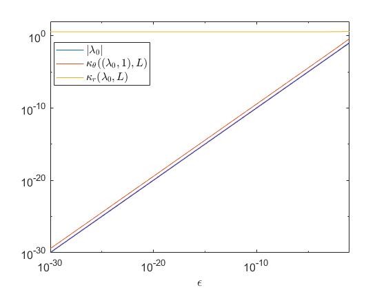
Fig. 1: Plot of $|\lambda_{0}|$, $\kappa_{\theta}((\lambda_{0},1),L)$ and $\kappa_{r}(\lambda_{0},L)$ against $\epsilon$ in Example 27.

In summary, we have proven that, as $\epsilon\to 0$, the pencil $L(\lambda)=\lambda B_{1}+B_{0}$ in Example 27 has well-conditioned matrix coefficients with very different norms, it has two eigenvalues close to 0 and they are both computable, since their non-homogeneous relative condition numbers are approximately 1. It is easy to check that $revL$ is an example of a pencil that has computable very large eigenvalues. As commented before, these pencils illustrate the only situation in which non-homogeneous eigenvalues with very small or large modulus can be accurately computed, which corresponds to pencils with highly unbalanced coefficients.

5 Conclusions

We have gathered together the definitions of (non-homogeneous and homogeneous) eigenvalue condition numbers of matrix polynomials that were scattered in the literature. We have also derived for the first time an exact formula to compute one of these condition numbers (the homogeneous condition number that is based on the chordal distance, also called Stewart-Sun condition number). On the one hand, we have determined that the two homogeneous condition numbers studied in this paper differ at most by a factor $\sqrt{k+1}$, where $k$ is the grade of the polynomial, and so are essentially equal in practice. Since the definition of the homogeneous condition number based on the chordal distance is considerably simpler, we believe that its use should be preferred among the homogeneous condition numbers. On the other hand, we have proved exact relationships between each of the non-homogeneous condition numbers and the homogeneous condition number based on the chordal distance. This result would allow us to extend results that have been proved for the non-homogeneous condition numbers to the homogeneous condition numbers (and vice versa). Besides, we have provided geometric interpretations of the factor that appears in these exact relationships, which explain transparently when and why the non-homogeneous condition numbers are much larger than the homogeneous ones. Finally, we have used these relationships to analyze for which cases the large and small non-homogeneous eigenvalues of a matrix polynomial are computable with some accuracy and we have seen that this is only possible in some very particular situations.

References

- [1] M. Berhanu, The polynomial eigenvalue problem. Thesis (Ph.D.) - The University of Manchester (United Kingdom). 2005. 221 pp. ISBN: 978-0355-47610-1.
- [2] J. P. Dedieu, Condition operators, condition numbers, and condition number theorem for the generalized eigenvalue problem, Linear Algebra Appl., 263 (1997), 1-24.
- [3] J.P. Dedieu and F. Tisseur, Perturbation theory for homogeneous polynomial eigenvalue problems, Linear Algebra Appl., 358 (2003), 71-94.
- [4] S. Hammarling, C.J. Munro, and F. Tisseur, An algorithm for the complete solution of quadratic eigenvalue problems, ACM Trans. Math. Softw., 39,3 (2013), 18:1-18:19.
- [5] N.J. Higham, D. S. Mackey, and F. Tisseur, The conditioning of linearizations of matrix polynomials, SIAM J. Matrix Anal. Appl., 28, 4 (2006), 1005-1028.
- [6] M. Shub and S. Smale, Complexity of Bezout’s theorem IV: Probability of success; extensions, SIAM J. Numer. Anal., 33,1 (1996), 128-148.
- [7] G. W. Stewart and J.-G. Sun, Matrix Perturbation Theory, Academic Press, Boston, 1990.
- [8] F. Tisseur, Backward error and condition of polynomial eigenvalue problems, Linear Algebra Appl., 309 (2000), 339-361.