Space-time multiscale model reduction for transport equations

Abstract

In this paper, we propose a space-time GMsFEM for transport equations. Multiscale transport equations occur in many geoscientific applications, which include subsurface transport, atmospheric pollution transport, and so on. Most of existing multiscale approaches use spatial multiscale basis functions or upscaling, and there are very few works that design space-time multiscale functions to solve the transport equation on a coarse grid. For the time dependent problems, the use of space-time multiscale basis functions offers several advantages as the spatial and temporal scales are intrinsically coupled. By using the GMsFEM idea with a space-time framework, one obtains a better dimension reduction taking into account features of the solutions in both space and time. In addition, the time-stepping can be performed using much coarser time step sizes compared to the case when spatial multiscale basis are used. Our scheme is based on space-time snapshot spaces and model reduction using space-time spectral problems derived from the analysis. We give the analysis for the well-posedness and the spectral convergence of our method. We also present some numerical examples to demonstrate the performance of the method. In all examples, we observe a good accuracy with a few basis functions.

1 Introduction

Transport processes in practical applications have multiscale nature. The convection term in the transport equation is governed by a flow velocity field, which can be described by the Darcy equation or the steady-state Stokes equation, and the convection velocity is typically highly heterogeneous and contains many scales. Because of the spatial and magnitude variations of the velocity field, the transport equation contains both spatial and temporal scales. For example, high velocity fields in thin channels introduce both spatial scales related to channel sizes and temporal scales related to velocity variations. These scales are tightly coupled in this example, as we deal with high convection in small channel like spatial regions.

Transport equations governed or dominated by convection processes occur in many geoscientific applications. Besides subsurface processes, the convection-dominated multiscale transport occurs in atmospheric sciences, where particles are transported by the air. Because atmospheric flows can have multiple scales, one deals with multiscale transport equations with space and time heterogeneities. Other geoscientific applications include the transport in vadoze zone hydrology and so on.

Numerical solutions for these transport equations can be expensive as we need to resolve both spatial and temporal scales. Some type of model reduction can be used to reduce the computational cost and achieve a certain degree accuracy at a very reduced cost. Model reduction techniques usually depend on a coarse grid approximation, which can be obtained by discretizing the problem on a coarse grid and choosing a suitable coarse-grid formulation of the problem. In the literature, several approaches have been developed to obtain the coarse-grid formulation, including upscaling methods [29, 22, 23, 20, 25, 3, 2, 27, 6, 8] and multiscale methods [19, 24, 17, 16, 4, 9, 5, 1]. Among these approaches, GMsFEM (Generalized Multiscale Finite Element Methods) [18, 12, 11, 10, 15, 7] provides a systematic way of adding degrees of freedom for problems with high contrast and multiple scales. Most of these approaches have been developed for diffusion dominated processes. Our goal is to extend these concepts to transport equations by designing appropriate space-time basis functions. We note that the proposed problems do not have scale separation and one can not represent the velocity field by a single “average” velocity field on a coarse grid [21, 28]. Appropriate number of coarse-grid parameters is needed to obtain accurate solutions.

In this paper, we propose a space-time GMsFEM for the transport equations. To do so, we start with a coarse space-time grid, which does not necessarily resolve the fine-scale heterogeneities. Then, we derive a space-time discontinuous Galerkin formulation, which uses upwinding for the convection term and the time derivative. The key component of the scheme is the basis functions, which are supported on space-time coarse elements. To construct the basis functions, we apply the general concept of GMsFEM. In particular, for each coarse space-time element, we first find the snapshot space. We consider two ways to compute the snapshot space. In our first approach, we solve the transport equation on each space-time coarse element with all possible initial and boundary conditions resolved on the underlying fine grid. In the second approach, we consider an oversampling strategy, in which we solve the transport equation on oversampled space-time regions. Next, we perform local model reduction procedure in order to obtain the offline space for the computation of the solution. In this step, we construct a local spectral problem defined on the snapshot space and identify dominant modes as the basis functions. We remark that the spectral problem takes care both the space and time structures, and is designed by our convergence analysis.

In the paper, we will present the detailed construction of the basis functions. In addition, we will give analysis for the well-posedness of the discrete system as well as the spectral convergence of the scheme. We have shown that the error is inversely proportional to the eigenvalues of the spectral problem. Furthermore, we illustrate the performance of our scheme by a couple of test cases. In both cases, we see that our scheme is able to produce accurate solutions with only a few multiscale basis functions. We also compare the performance with the use of space-time polynomial basis functions, and show that our scheme is able to capture the scales of the solutions with very few degrees of freedoms. We remark that the use of space-time basis functions offers some advantages over the use of spatial multiscale basis functions. In particular, space-time basis functions are able to capture the scales in both space and time, when they are tightly coupled. The latter is the case in the applications of interest. Besides, space-time approaches allow the scheme to update the solution with a coarser time step size. The success of the space-time basis functions is also illustrated by a work for parabolic equations [14].

Numerical results are presented in the paper. We consider the velocity field obtained by solving flow equation in highly heterogeneous, high-contrast media. The media contains high-permeability channels and inclusions, which introduce several time scales. We solve the transport equation with some choices of boundary and initial conditions and compare the fine-grid solution against the multiscale solution with various number of basis functions. Our numerical results show that with a few basis functions, we can obtain accurate results.

The paper is organized as follows. In Section 2, we present the construction of the method, including the space-time formulation and basis function constructions, and prove the well-posedness of the discrete system. In Section 3, we prove the spectral convergence of the scheme. We illustrate the performance of the scheme by some numerical examples in Section 4. The paper ends with a conclusion.

2 Space-time GMsFEM

In this section, we will give the construction of our space-time GMsFEM for transport equations. First, we present some basic notations and the coarse grid formulation in Section 2.1. Then, we present the constructions of the space-time multiscale snapshot functions and basis functions in Section 2.2.

2.1 Preliminaries

Let $\Omega$ be a bounded domain in $\mathbb{R}^{2}$ with a Lipschitz boundary $\partial\Omega$ with unit normal vector $\mathbf{n}$, and $[0,T]$ $(T>0)$ be a time interval. In this paper, we consider the following transport equation:

$$\begin{split}\frac{\partial u}{\partial t}+\mathbf{v}\cdot\nabla u&=0\quad\quad\quad\text{in}\;\Omega\times(0,T),\\ u&=g\quad\quad\quad\text{on}\;\Gamma^{-}\times(0,T),\\ u(x,0)&=u_{0}(x)\,\quad\text{in}\;\Omega\times\left\{t=0\right\},\end{split}$$ (1)

where $\mathbf{v}$ is a given divergence-free velocity field, $g$ is the inflow boundary data, $u_{0}(x)$ is initial condition, $\Gamma^{-}=\left\{x\in\partial\Omega\,|\,\mathbf{v}\cdot\mathbf{n}<0\right\}$ is the inflow boundary and $\Gamma^{+}=\left\{x\in\partial\Omega\,|\,\mathbf{v}\cdot\mathbf{n}>0\right\}$ is the outflow boundary. We remark that the method presented in this paper can be applied to 3D problems.

The goal of this paper is to develop a space-time generalized multiscale finite element method. The method is motivated by the space-time finite element framework. First, a space-time variational formulation is defined. Then some space-time multiscale basis functions are constructed. The constructions of the multiscale basis functions follow two general steps. In the first step, we will construct space-time snapshot functions in order to build a set of possible modes of the solution. The snapshot functions are obtained by solving local problem on coarse space-time cells. We consider the use of oversampling technique with the aim of reducing the offline cost. In the second step, we will construct multiscale basis functions. To do so, we design a suitable spectral problem defined in the snapshot space, and use the first few dominant eigenfunctions as the basis functions. We note that the spectral problems take both space and time into account. By using the space-time multiscale basis functions, we obtain a reduced model which takes into account the variations of the solutions in both space and time, and thus produces accurate solution for the transport equation in heterogeneous media.

Let $\mathcal{T}^{h}$ be a partition of the domain $\Omega$ into fine finite elements. Here $h>0$ is the fine mesh size. The coarse partition, $\mathcal{T}^{H}$ of the domain $\Omega$, is formed such that each element in $\mathcal{T}^{H}$ is a connected union of fine-grid blocks. More precisely, $\forall K_{j}\in\mathcal{T}^{H},\;K_{j}=\cup_{F\in I_{j}}F$ for some $I_{j}\subset\mathcal{T}^{h}$. The quantity $H>0$ is the coarse mesh size. We will consider rectangular coarse elements and the methodology can be used with general coarse elements. An illustration of the mesh notations is shown in Figure 1 (left).

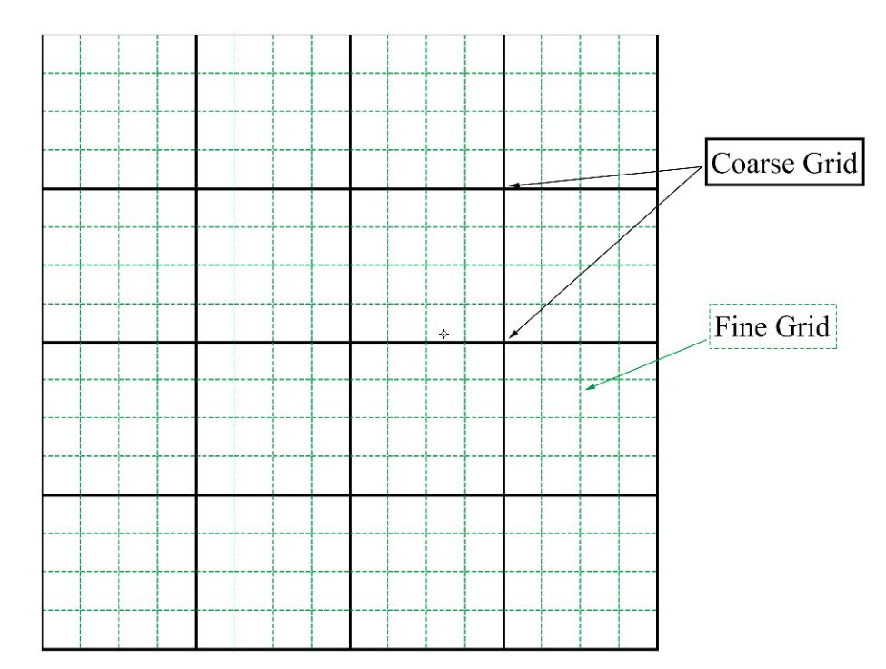
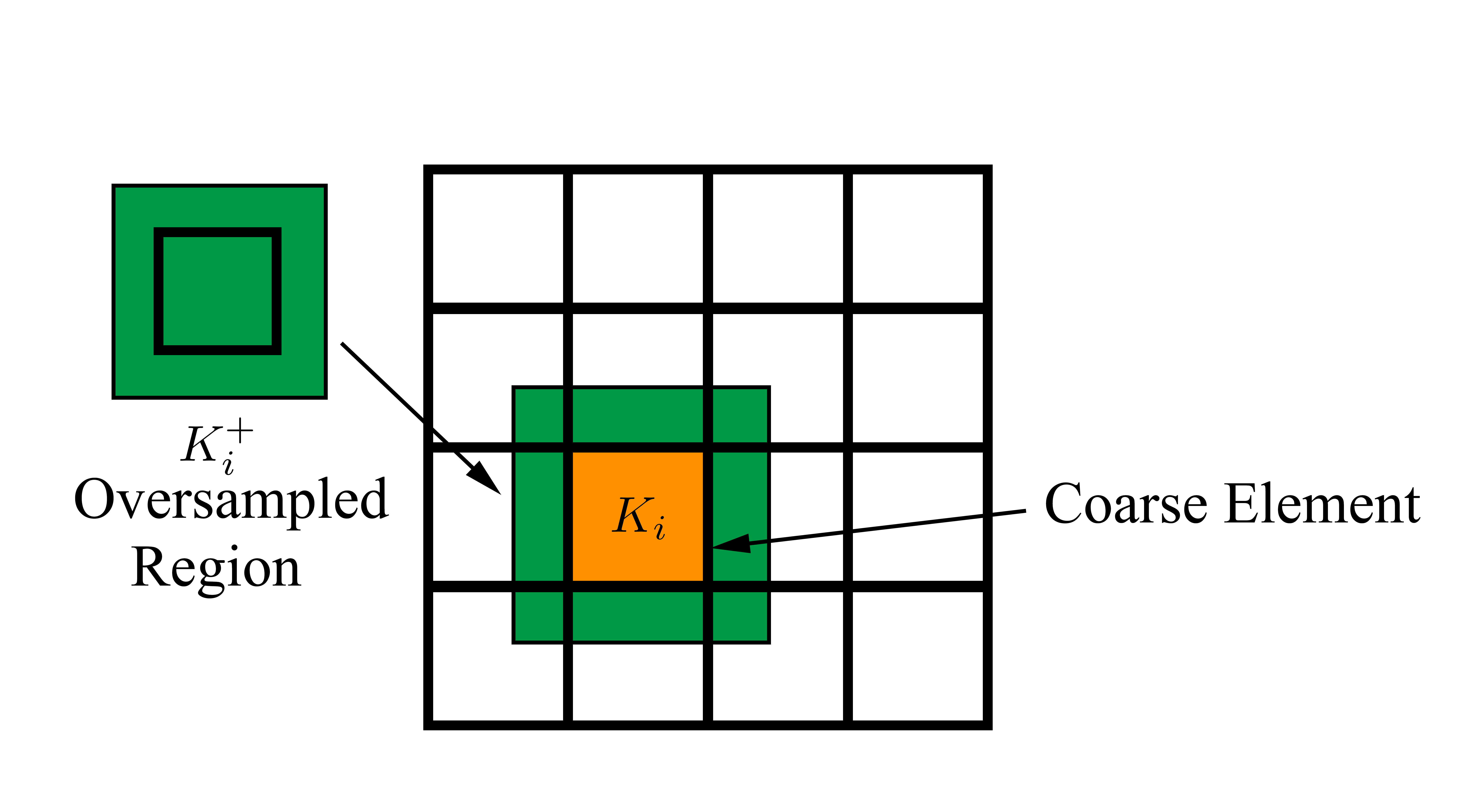
Figure 1: Left: an illustration of fine and coarse grids. Right: an illustration of a coarse neighborhood and a coarse element.

Next, let $\mathcal{T}^{T}=\{(T_{n-1},T_{n})|1\leq n\leq N\}$ be a coarse partition of $(0,T)$, where

$$0=T_{0}<T_{1}<T_{2}<\cdots<T_{N}=T$$

and we define a fine partition $\mathcal{T}^{t}$ of $(0,T)$ by refining the partition $\mathcal{T}^{T}$, that is $\mathcal{T}^{t}=\{(T_{i-\frac{1}{r}},T_{i})|i=\frac{1}{r},\frac{2}{r},\cdots,N-\frac{1}{r},N\}$, where

$$0=T_{0}<T_{\frac{1}{r}}<\cdots<T_{1-\frac{1}{r}}<T_{1}<T_{1+\frac{1}{r}}<\cdots<T_{N}=T$$

To fix the notations, we define the finite element space $V_{h}$ with respect to $\mathcal{T}^{h}\times(0,T)$ as a space consists of piecewise linear functions in fine grid. Here we introduce two types of $V_{h}$.

2.1.1 CG in coarse cell

We use the term ”coarse cell” to represent $K\times(T_{n-1},T_{n})$ where $K$ is a coarse element in space, and $(T_{n-1},T_{n})$ is a coarse time interval. In this case, all functions in $V_{h}$ are continuous in each coarse cell, that is

$$V_{h}= \left\{v\in L^{2}((0,T);\Omega)\,|\,v=\phi(x)\psi(t)\text{ where }\phi|_{K}\in Q_{1}(K)\;\forall K\in\mathcal{T}^{h},\,\phi|_{K}\in C^{0}(K)\;\forall K\in\mathcal{T}^{H},\right.$$

$$\left.\psi|_{\tau}\in P_{1}(\tau)\;\forall\tau\in\mathcal{T}^{t},\,\text{ and }\psi|_{\tau}\in C^{0}(\tau)\;\forall\tau\in\mathcal{T}^{T}\right\}.$$

Next, we let $\mathcal{E}_{H}$ be the collection of all coarse edges, and $\mathcal{E}_{H}^{0}=\mathcal{E}_{H}\backslash\partial\Omega$. For the value on a coarse edge, which is shared by two coarse blocks $K_{i}$ and $K_{j}$, if $K_{i}$ is the upwind block, define $w^{+}=w|_{K_{i}}$ and $w^{-}=w|_{K_{j}}$ for the corresponding downwind value. Figure 2 gives an illustration.

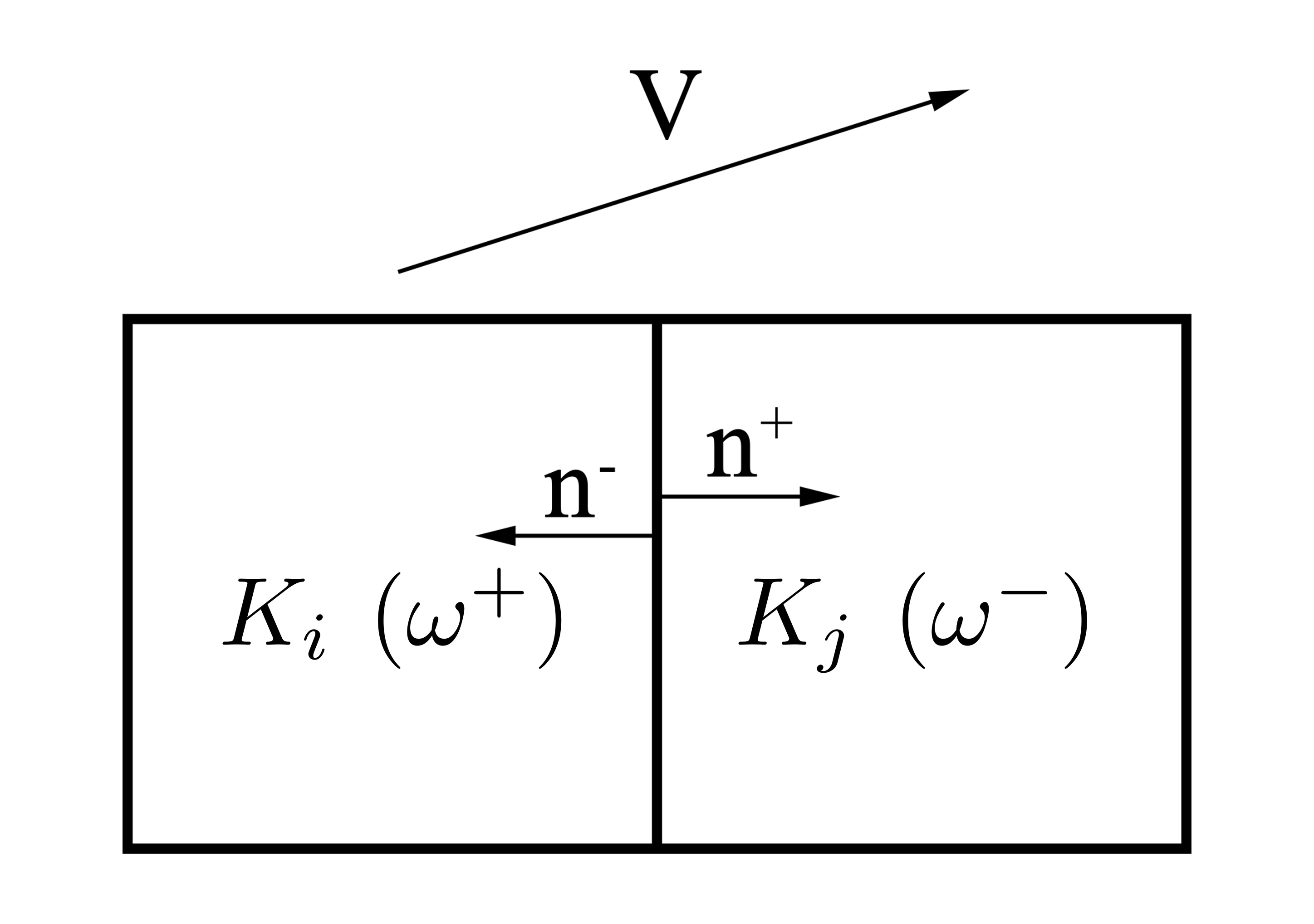
Figure 2: An illustration of upwind and downwind blocks.

The fine-scale solution $u_{h}\in V_{h}$ is obtained by solving the following variational problem

$$\begin{split}\int_{0}^{T}\int_{\Omega}\left(\frac{\partial u_{h}}{\partial t}w-u_{h}\nabla w\cdot\mathbf{v}\right)+\int_{0}^{T}\sum_{e\in\mathcal{E}_{H}^{0}}\int_{e}u_{h}^{+}[w]\cdot\mathbf{v}+\int_{0}^{T}\sum_{e\in{\Gamma^{+}}}\int_{e}u_{h}w\mathbf{v}\cdot\mathbf{n}\\ -\sum_{n=0}^{N-1}\int_{\Omega}\left[\left[u_{h}(x,T_{n})\right]\right]w(x,T_{n}^{+})=\int_{0}^{T}u_{0}(x)w(x,T_{n}^{+})-\int_{0}^{T}\sum_{e\in{\Gamma^{-}}}\int_{e}gw\mathbf{v}\cdot\mathbf{n},\quad\forall w\in V_{h}.\end{split}$$ (2)

where $[\cdot]$ is the jump operator in space defined by

$$[w]=\left\{\begin{matrix}w^{-}\mathbf{n}^{-}+w^{+}\mathbf{n}^{+}&\text{on }\mathcal{E}_{H}^{0},\\ w^{-}\mathbf{n}^{-}&\text{on }\Gamma^{-},\\ w^{+}\mathbf{n}^{+}&\text{on }\Gamma^{+}.\end{matrix}\right.$$ (3)

And $[[\cdot]]$ is the jump operator in time defined by

$$\left[\left[u_{h}(x,T_{n})\right]\right]=\left\{\begin{matrix}u_{h}(x,T_{0}^{+})&\text{for }n=0,\\ u_{h}(x,T_{n}^{+})-u_{h}(x,T_{n}^{-})&\text{for }n>0.\end{matrix}\right.$$ (4)

The above equation uses an upwind approximation in $\mathbf{v}\cdot\nabla u$ term, and is motivated by [14] and [26]. We assume that the fine mesh size $h$ is small enough so that the fine-scale solution $u_{h}$ is close enough to the exact solution. We will skip the discussion on the well-posedness of (2) since it is similar to that of the coarse scale system to be presented. We will also skip the approximation property of the fine-scale solver since it is standard (see for example [26]).

We note that the purpose of this paper is to find a multiscale solution $u_{H}$ that is a good approximation of the fine-scale solution $u_{h}$.

Now we present the general idea of GMsFEM. We will use the space-time finite element method to solve the system (1) on the coarse grid. We will use a similar framework as (2). That is, we find $u_{H}\in V_{H}$ such that

$$\begin{split}\int_{0}^{T}\int_{\Omega}\left(\frac{\partial u_{H}}{\partial t}w-u_{H}\nabla w\cdot\mathbf{v}\right)+\int_{0}^{T}\sum_{e\in\mathcal{E}_{H}^{0}}\int_{e}u_{H}^{+}[w]\cdot\mathbf{v}+\int_{0}^{T}\sum_{e\in{\Gamma^{+}}}\int_{e}u_{H}w\mathbf{v}\cdot\mathbf{n}\\ +\sum_{n=0}^{N-1}\int_{\Omega}\left[\left[u_{H}(x,T_{n})\right]\right]w(x,T_{n}^{+})=\int_{\Omega}u_{0}(x)w(x,T_{0}^{+})-\int_{0}^{T}\sum_{e\in{\Gamma^{-}}}\int_{e}gw\mathbf{v}\cdot\mathbf{n}\quad\forall w\in V_{H},\end{split}$$ (5)

where $V_{H}$ is the multiscale finite element space which will be introduced in the following subsections.
 To avoid a large computational cost associated with solving the equation (5), we divide the computational domain. We assume the solution space $V_{H}$ is a direct sum of the spaces only containing the functions defined on one single coarse time interval $(T_{n-1},T_{n})$. We decompose the problem (5) into a sequence of problems and find the solution $u_{H}$ in each time interval sequentially. Our coarse space will be constructed in each time interval

$$V_{H}=\bigoplus_{n=1}^{N}V_{H}^{(n)},$$

where $V_{H}^{(n)}$ only contains the functions having zero values in the time interval $(0,T)$ except $(T_{n-1},T_{n})$, namely $\forall v\in V_{H}^{(n)}$,

$$v(\cdot,t)=0\text{ for }t\in(0,T)\backslash(T_{n-1},T_{n}).$$

The equation (5) can be decomposed into the following problem: find $u_{H}^{(n)}\in V_{H}^{(n)}$ (where $V_{H}^{(n)}$ will be defined later) satisfying

$$\begin{split}&\int_{T_{n-1}}^{T_{n}}\int_{\Omega}\left(\frac{\partial u_{H}^{(n)}}{\partial t}w-u_{H}^{(n)}\nabla w\cdot\mathbf{v}\right)+\int_{T_{n-1}}^{T_{n}}\sum_{e\in\mathcal{E}_{H}^{0}}\int_{e}u_{H}^{(n)+}[w]\cdot\mathbf{v}\\ &+\int_{T_{n-1}}^{T_{n}}\sum_{e\in{\Gamma^{+}}}\int_{e}u_{H}^{(n)}w\mathbf{v}\cdot\mathbf{n}+\int_{\Omega}u_{H}^{(n)}(x,T_{n-1}^{+})w(x,T_{n-1}^{+})\\ =&\int_{\Omega}f_{H}^{(n)}(x)w(x,T_{n-1}^{+})-\int_{T_{n-1}}^{T_{n}}\sum_{e\in{\Gamma^{-}}}\int_{e}gw\mathbf{v}\cdot\mathbf{n},\quad\forall w\in V_{H}^{(n)},\end{split}$$ (6)

where

$$f_{H}^{(n)}(x)=\left\{\begin{matrix}u_{H}^{(n-1)}(x,T_{n-1}^{-})&\text{for}&n\geq 2\\ u_{0}&\text{for}&n=1.\end{matrix}\right.$$

Then the solution $u_{H}$ is the direct sum of all these $u_{H}^{(n)}$’s, that is $u_{H}=\bigoplus_{n=1}^{N}u_{H}^{(n)}.$ Next, we motivate the use of space-time multiscale basis functions by comparing it to space multiscale basis functions. Let $\left\{T_{n-1},T_{n-1+\frac{1}{r}},\cdots,T_{n-\frac{1}{r}},T_{n}\right\}$ be $r$ fine time steps in $(T_{n-1},T_{n})$. The solution can be represented as $u_{H}^{(n)}=\sum_{l,i}c_{l,i}\phi_{l}^{K_{i}}(x,t)$ in the interval $(T_{n-1},T_{n})$, where the number of coefficients $c_{l,i}$ is related to the size of the reduced system in space-time interval. If we use spatial multiscale basis functions, these multiscale basis functions are constructed at each fine time interval $(T_{p-\frac{1}{r}},T_{p})$, denoted by $\phi_{l}^{K_{i}}(x,T_{p})$. The solution $u_{H}$ spanned by these basis functions will have a larger dimension since each time interval is represented by multiscale basis functions.

2.1.2 DG in coarse cell

In this case, all functions in $V_{h}$ could be discontinuous in each coarse cell, that is

$$V_{h}=\left\{v\in L^{2}((0,T);\Omega)\,|\,v=\phi(x)\psi(t)\text{ where }\phi|_{K}\in Q_{1}(K)\;\forall K\in\mathcal{T}^{h},\,\psi|_{\tau}\in P_{1}(\tau)\;\forall\tau\in\mathcal{T}^{t}\right\}.$$

We let $\mathcal{E}_{h}$ be the collection of all fine edges, and $\mathcal{E}_{h}^{0}=\mathcal{E}_{h}\backslash\partial\Omega$. The fine-scale solution $u_{h}\in V_{h}$ is obtained by solving the following variational problem

$$\begin{split}\int_{0}^{T}\int_{\Omega}\left(\frac{\partial u_{h}}{\partial t}w-u_{h}\nabla w\cdot\mathbf{v}\right)+\int_{0}^{T}\sum_{e\in\mathcal{E}_{h}^{0}}\int_{e}u_{h}^{+}[w]\cdot\mathbf{v}+\int_{0}^{T}\sum_{e\in{\Gamma^{+}}}\int_{e}u_{h}w\mathbf{v}\cdot\mathbf{n}\\ +\sum_{p=0}^{N-\frac{1}{r}}\int_{\Omega}\left[\left[u_{h}(x,T_{p})\right]\right]w(x,T_{p}^{+})=\int_{\Omega}u_{0}(x)w(x,T_{0}^{+})-\int_{0}^{T}\sum_{e\in{\Gamma^{-}}}\int_{e}gw\mathbf{v}\cdot\mathbf{n},\quad\forall w\in V_{h},\end{split}$$ (7)

where the jump operators $[\cdot]$ and $\left[[\cdot]\right]$ have similar definition to equation (3) and (4).

As for GMsFEM, we find $u_{H}\in V_{H}$ such that

$$\begin{split}\int_{0}^{T}\int_{\Omega}\left(\frac{\partial u_{H}}{\partial t}w-u_{H}\nabla w\cdot\mathbf{v}\right)+\int_{0}^{T}\sum_{e\in\mathcal{E}_{h}^{0}}\int_{e}u_{H}^{+}[w]\cdot\mathbf{v}+\int_{0}^{T}\sum_{e\in{\Gamma^{+}}}\int_{e}u_{H}w\mathbf{v}\cdot\mathbf{n}\\ +\sum_{p=0}^{N-\frac{1}{r}}\int_{\Omega}\left[\left[u_{H}(x,T_{p})\right]\right]w(x,T_{p}^{+})=\int_{\Omega}u_{0}(x)w(x,T_{0}^{+})-\int_{0}^{T}\sum_{e\in{\Gamma^{-}}}\int_{e}gw\mathbf{v}\cdot\mathbf{n},\quad\forall w\in V_{h},\end{split}$$ (8)

The equation (8) can be decomposed into the following problem: find $u_{H}^{(n)}\in V_{H}^{(n)}$ (where $V_{H}^{(n)}$ will be defined later) satisfying

$$\begin{split}&\int_{T_{n-1}}^{T_{n}}\int_{\Omega}\left(\frac{\partial u_{H}^{(n)}}{\partial t}w-u_{H}^{(n)}\nabla w\cdot\mathbf{v}\right)+\int_{T_{n-1}}^{T_{n}}\sum_{e\in\mathcal{E}_{h}^{0}}\int_{e}u_{H}^{(n)+}[w]\cdot\mathbf{v}+\int_{T_{n-1}}^{T_{n}}\sum_{e\in{\Gamma^{+}}}\int_{e}u_{H}^{(n)}w\mathbf{v}\cdot\mathbf{n}\\ &+\int_{\Omega}u_{H}^{(n)}(x,T_{n-1}^{+})w(x,T_{n-1}^{+})+\sum_{p=n-1+\frac{1}{r}}^{n-\frac{1}{r}}\int_{\Omega}\left[\left[u_{H}^{(n)}(x,T_{p})\right]\right]w(x,T_{p}^{+})\\ =&\int_{\Omega}f_{H}^{(n)}(x)w(x,T_{n-1}^{+})-\int_{T_{n-1}}^{T_{n}}\sum_{e\in{\Gamma^{-}}}\int_{e}gw\mathbf{v}\cdot\mathbf{n},\quad\forall w\in V_{H}^{(n)},\end{split}$$ (9)

2.2 Construction of offline basis functions

In this section, we will give the constructions of multiscale basis functions. In Section 2.2.1, we will present the construction of the snapshot space. To do so, we will solve the transport equation on coarse space-time cells with suitable initial and boundary conditions. This process will provide a set of functions which are able to span the fine-scale solution with high accuracy. We will also consider the use of the oversampling technique by solving the transport equation on a domain larger then the target coarse space-time cell. Next, in Section 2.2.2, we will present the construction of our multiscale basis functions. The construction is based on the design of a local spectral problem which can identify important modes in the snapshot space. Our choice of spectral problem is based on our convergence analysis given later.

2.2.1 Snapshot Space

Let $K_{i}$ be a given coarse element in space. Consider the coarse time interval $(T_{n-1},T_{n})$. We will construct a snapshot space $V_{\text{snap}}^{i(n)}$ containing functions defined on coarse cell $K_{i}\times(T_{n-1},T_{n})$. A spectral problem is then solved in the snapshot space to extract the dominant modes in the snapshot space. These dominant modes are the offline multiscale basis functions and the resulting reduced space is called the offline space. We will present two choices of $V_{\text{snap}}^{i(n)}$.

The first choice for the snapshot spaces consists of solving the transport equation on the target space-time coarse cell $K_{i}\times(T_{n-1},T_{n})$ for all possible boundary conditions. In particular, we define the $j$-th snapshot function $\psi_{j}$ as the solution to the following problem

$$\left\{\begin{array}[]{rl}\frac{\partial\psi_{j}}{\partial t}+\mathbf{v}\cdot\nabla\psi_{j}=0&\text{in}\quad K_{i}\times(T_{n-1},T_{n}),\\ \psi_{j}(x,t)=\delta_{ij}(x,t)&\text{on}\quad\partial(K_{i}\times(T_{n-1},T_{n})).\end{array}\right.$$ (12)

Here $\delta_{ij}(x,t)$ is a fine-grid delta function and $\partial(K_{i}\times(T_{n-1},T_{n}))$ denotes the boundaries $t=T_{n-1}$ and on $(\partial K_{i})^{-}\times(T_{n-1},T_{n})$. Then $V_{\text{snap}}^{i(n)}$ consists of all $\psi_{j}$’s.

To improve the accuracy of the solution, we can take an advantage of oversampling concepts. We denote by $K_{i}^{+}$ the oversampled space region of $K_{i}\subset K_{i}^{+}$, defined by adding several fine- or coarse-grid layers around $K_{i}$ (see Figure 1). Also, we define $(T_{n-1}^{*},T_{n})$ as the left-side oversampled time region for $(T_{n-1},T_{n})$. We generate our second choice of the snapshot space on the oversampled space-time region $K_{i}^{+}\times(T_{n-1}^{*},T_{n})$ by solving

$$\left\{\begin{array}[]{rl}\frac{\partial\psi_{j}^{+}}{\partial t}+\mathbf{v}\cdot\nabla\psi_{j}^{+}=0&\text{in}\quad K_{i}^{+}\times(T_{n-1}^{*},T_{n})\\ \psi_{j}^{+}(x,t)=\delta_{ij}(x,t)&\text{on}\quad\partial(K_{i}^{+}\times(T_{n-1}^{*},T_{n})).\end{array}\right.$$ (15)

Then $V_{\text{snap}}^{i(n)+}$ consists of all $\psi_{j}^{+}$’s, and $V_{\text{snap}}^{i(n)}$ consists of all $\psi_{j}=\psi_{j}^{+}|_{K_{i}}$’s. Finally, $V_{\text{snap}}^{(n)}$ is spanned by all functions in each $V_{\text{snap}}^{i(n)}$, that is

$$V_{\text{snap}}^{(n)}=\bigoplus_{K_{i}}V_{\text{snap}}^{i(n)}.$$

We will use the second choice of the snapshot space in the rest of the paper.

For the case in Section 2.1.1, we define snapshot solution $u_{\text{snap}}^{(n)}\in V_{\text{snap}}^{(n)}$ such that

$$\begin{split}&\int_{T_{n-1}}^{T_{n}}\int_{\Omega}\left(\frac{\partial u_{\text{snap}}^{(n)}}{\partial t}w-u_{\text{snap}}^{(n)}\nabla w\cdot\mathbf{v}\right)+\int_{T_{n-1}}^{T_{n}}\sum_{e\in\mathcal{E}_{H}^{0}}\int_{e}u_{\text{snap}}^{(n)+}[w]\cdot\mathbf{v}+\int_{T_{n-1}}^{T_{n}}\sum_{e\in{\Gamma^{+}}}\int_{e}u_{\text{snap}}^{(n)}w\mathbf{v}\cdot\mathbf{n}\\ &+\int_{\Omega}u_{\text{snap}}^{(n)}(x,T_{n-1}^{+})w(x,T_{n-1}^{+})+\sum_{n=0}^{N-1}\int_{\Omega}\left[\left[u_{\text{snap}}^{(n)}(x,T_{n})\right]\right]w(x,T_{n}^{+})\\ =&\int_{\Omega}f_{\text{snap}}^{(n)}(x)w(x,T_{n-1}^{+})-\int_{T_{n-1}}^{T_{n}}\sum_{e\in{\Gamma^{-}}}\int_{e}gw\mathbf{v}\cdot\mathbf{n},\quad\forall w\in V_{\text{snap}}^{(n)},\end{split}$$ (16)

where

$$f_{\text{snap}}^{(n)}(x)=\left\{\begin{matrix}u_{\text{snap}}^{(n-1)}(x,T_{n-1}^{-})&\text{for}&n\geq 2\\ u_{0}&\text{for}&n=1.\end{matrix}\right.$$

And for the case in Section 2.1.2, we define snapshot solution $u_{\text{snap}}^{(n)}\in V_{\text{snap}}^{(n)}$ such that

$$\begin{split}&\int_{T_{n-1}}^{T_{n}}\int_{\Omega}\left(\frac{\partial u_{\text{snap}}^{(n)}}{\partial t}w-u_{\text{snap}}^{(n)}\nabla w\cdot\mathbf{v}\right)+\int_{T_{n-1}}^{T_{n}}\sum_{e\in\mathcal{E}^{0}}\int_{e}u_{\text{snap}}^{(n)+}[w]\cdot\mathbf{v}+\int_{T_{n-1}}^{T_{n}}\sum_{e\in{\Gamma^{+}}}\int_{e}u_{\text{snap}}^{(n)}w\mathbf{v}\cdot\mathbf{n}\\ &+\int_{\Omega}u_{\text{snap}}^{(n)}(x,T_{n-1}^{+})w(x,T_{n-1}^{+})+\sum_{p=n-1+\frac{1}{r}}^{n-\frac{1}{r}}\int_{\Omega}\left[\left[u_{\text{snap}}^{(n)}(x,T_{p})\right]\right]w(x,T_{p}^{+})\\ =&\int_{\Omega}f_{\text{snap}}^{(n)}(x)w(x,T_{n-1}^{+})-\int_{T_{n-1}}^{T_{n}}\sum_{e\in{\Gamma^{-}}}\int_{e}gw\mathbf{v}\cdot\mathbf{n},\quad\forall w\in V_{\text{snap}}^{(n)},\end{split}$$ (17)

2.2.2 Offline Space

To obtain the offline multiscale basis functions, we need to perform a space reduction by appropriate spectral problems. Motivated by our later convergence analysis, we adopt the following spectral problem on $K_{i}^{+}\times(T_{n-1}^{*},T_{n})$: find $\left(\phi^{+},\lambda\right)\in V_{\text{snap}}^{i(n)+}\times\mathbb{R}$ such that

$$a_{n}(\phi^{+},\eta^{+})=\lambda s_{n}(\phi^{+},\eta^{+}),\;\;\;\forall\eta^{+}\in V_{\text{snap}}^{i(n)+},$$

where the bilinear operators $a_{n}(\phi^{+},\eta^{+})$ and $s_{n}(\phi^{+},\eta^{+})$ are defined as follow:
For the case in Section 2.1.1:

$$a_{n}(\phi^{+},\eta^{+})= \int_{T_{n-1}^{*}}^{T_{n}}\int_{K_{i}^{+}}\nabla\phi^{+}\cdot\nabla\eta^{+},$$

$$s_{n}(\phi^{+},\eta^{+})= \frac{1}{2}\left(\int_{K_{i}}\phi^{+}(x,T_{n-1}^{+})\eta^{+}(x,T_{n-1}^{+})+\int_{K_{i}}\phi^{+}(x,T_{n}^{-})\eta^{+}(x,T_{n}^{-})+\int_{T_{n-1}}^{T_{n}}\int_{\partial{K_{i}}}\left|\mathbf{v}\cdot\mathbf{n}\right|\phi^{+}\eta^{+}\right).$$

For the case in Section 2.1.2:

$$a_{n}(\phi,\eta)= \frac{1}{2}\left(\sum_{p=n-1+\frac{1}{r}}^{n-\frac{1}{r}}\int_{K_{i}}\left[\left[\phi(x,T_{p})\right]\right]\left[\left[\eta(x,T_{p})\right]\right]+\int_{T_{n-1}}^{T_{n}}\sum_{e\in\mathcal{E}^{0}(K_{i})}\int_{e}\left|\mathbf{v}\cdot\mathbf{n}\right|[\phi][\eta]\right),$$

$$s_{n}(\phi,\eta)= \frac{1}{2}\left(\int_{K_{i}}\phi(x,T_{n-1}^{+})\eta(x,T_{n-1}^{+})+\int_{K_{i}}\phi(x,T_{n}^{-})\eta(x,T_{n}^{-})\right.$$

$$\left.+\sum_{p=n-1+\frac{1}{r}}^{n-\frac{1}{r}}\int_{K_{i}}\left(\phi(x,T_{p}^{-})\eta(x,T_{p}^{-})+\phi(x,T_{p}^{+})\eta(x,T_{p}^{+})\right)+\int_{T_{n-1}}^{T_{n}}\sum_{\tau\subset K_{i}}\int_{\partial\tau}\left|\mathbf{v}\cdot\mathbf{n}\right|\phi\eta\right).$$

We arrange the eigenfunctions $\phi_{j}^{+}$’s in ascending order of the corresponding eigenvalues $\lambda_{j}$’s, and obtain $\phi_{j}$’s on the target region $K_{i}\times(T_{n-1},T_{n})$ by restricting $\phi_{j}^{+}$’s onto $K_{i}\times(T_{n-1},T_{n})$. Then we select first $L_{i}$ functions $\phi_{1},\phi_{2},...,\phi_{L_{i}}$ to construct local offline space $V_{H}^{i(n)}$, and perform POD to remove linearly dependent functions. We define $L=\max_{i}L_{i}$. Finally $V_{H}^{(n)}$ is spanned by all functions in each $V_{H}^{i(n)}$, that is

$$V_{H}^{(n)}=\bigoplus_{K_{i}}V_{H}^{i(n)}.$$

This is the approximation space we used to solve the system (1) using the formulation (9).

3 Convergence Analysis

In this section, we will analyze the convergence of our proposed method. We will only consider the case in Section 2.1.1, the case in Section 2.1.2 will be similar.

First, we will define the following norms

$$\left\|u\right\|_{V^{(n)}}^{2}=\frac{1}{2}\left(\int_{\Omega}u^{2}(x,T_{n-1}^{+})+\int_{\Omega}u^{2}(x,T_{n}^{-})+\int_{T_{n-1}}^{T_{n}}\sum_{e\in\mathcal{E}_{H}}\int_{e}\left|\mathbf{v}\cdot\mathbf{n}\right|[u]^{2}\right)$$

and

$$\left\|u\right\|_{W^{(n)}}^{2}=\frac{1}{2}\left(\int_{\Omega}u^{2}(x,T_{n}^{-})+\int_{\Omega}u^{2}(x,T_{n-1}^{+})+\int_{T_{n-1}}^{T_{n}}\sum_{K_{i}}\int_{\partial K_{i}}\left|\mathbf{v}\cdot\mathbf{n}\right|u^{2}\right).$$

We will first show that the problem (6) is well-posed. Then we will prove a best approximation property. Finally, we will prove an error bound of our method. To begin our convergence analysis, we write (6) as

$$a(u_{H}^{(n)},w)=F(w)$$

where

$$\begin{split}a(u,w)=&\int_{T_{n-1}}^{T_{n}}\int_{\Omega}\left(\frac{\partial u}{\partial t}w-u\nabla w\cdot\mathbf{v}\right)+\int_{T_{n-1}}^{T_{n}}\sum_{e\in\mathcal{E}_{H}^{0}}\int_{e}u^{+}[w]\cdot\mathbf{v}\\ &+\int_{T_{n-1}}^{T_{n}}\sum_{e\in{\Gamma^{+}}}\int_{e}uw\mathbf{v}\cdot\mathbf{n}+\int_{\Omega}u(x,T_{n-1}^{+})w(x,T_{n-1}^{+})\end{split}$$

and

$$F(w)=\int_{\Omega}f_{H}^{(n)}(x)w(x,T_{n-1}^{+})-\int_{T_{n-1}}^{T_{n}}\sum_{e\in{\Gamma^{-}}}\int_{e}gw\mathbf{v}\cdot\mathbf{n}.$$

In the following theorem, we prove the well-posedness of the scheme (6).

Theorem 1.

The space-time GMsFEM (6) has a unique solution. In addition, we have the following coercivity result

$$a(u,u)=\left\|u\right\|_{V^{(n)}}^{2},\quad\forall u\in V_{\text{snap}}^{(n)}.$$

Proof.

Since the system (6) is a square linear system, it suffices to prove that if $a(\widehat{u},w)=0$ for any $w\in V_{H}^{(n)}$, then $\widehat{u}=0$. To prove this, we will show that $a(u,u)=\left\|u\right\|_{V^{(n)}}^{2}$ for all $u\in V_{\text{snap}}^{(n)}$.

By direct calculations, we have

$$a(u,u)= \int_{T_{n-1}}^{T_{n}}\int_{\Omega}\left(\frac{\partial u}{\partial t}u-u\nabla u\cdot\mathbf{v}\right)+\int_{T_{n-1}}^{T_{n}}\sum_{e\in\mathcal{E}_{H}^{0}}\int_{e}u^{+}[u]\cdot\mathbf{v}$$

$$+\int_{T_{n-1}}^{T_{n}}\sum_{e\in{\Gamma^{+}}}\int_{e}u^{2}\mathbf{v}\cdot\mathbf{n}+\int_{\Omega}u^{2}(x,T_{n-1}^{+})$$

$$= \frac{1}{2}\int_{\Omega}\left(u^{2}(x,T_{n}^{-})-u^{2}(x,T_{n-1}^{+})\right)-\frac{1}{2}\int_{T_{n-1}}^{T_{n}}\sum_{K_{i}}\int_{\partial K_{i}}u^{2}\mathbf{v}\cdot\mathbf{n}$$

$$+\int_{T_{n-1}}^{T_{n}}\sum_{e\in\mathcal{E}_{H}^{0}}\int_{e}u^{+}[u]\cdot\mathbf{v}+\int_{T_{n-1}}^{T_{n}}\sum_{e\in{\Gamma^{+}}}\int_{e}u^{2}\mathbf{v}\cdot\mathbf{n}+\int_{\Omega}u^{2}(x,T_{n-1}^{+})$$

$$= \frac{1}{2}\int_{\Omega}\left(u^{2}(x,T_{n}^{-})+u^{2}(x,T_{n-1}^{+})\right)-\frac{1}{2}\int_{T_{n-1}}^{T_{n}}\sum_{K_{i}}\int_{\partial K_{i}}u^{2}\mathbf{v}\cdot\mathbf{n}$$

$$+\int_{T_{n-1}}^{T_{n}}\sum_{e\in\mathcal{E}_{H}^{0}}\int_{e}u^{+}[u]\cdot\mathbf{v}+\int_{T_{n-1}}^{T_{n}}\sum_{e\in{\Gamma^{+}}}\int_{e}u^{2}\mathbf{v}\cdot\mathbf{n}.$$

Since

$$-\frac{1}{2}\int_{T_{n-1}}^{T_{n}}\sum_{K_{i}}\int_{\partial K_{i}}u^{2}\mathbf{v}\cdot\mathbf{n}+\int_{T_{n-1}}^{T_{n}}\sum_{e\in\mathcal{E}_{H}^{0}}\int_{e}u^{+}[u]\cdot\mathbf{v}+\int_{T_{n-1}}^{T_{n}}\sum_{e\in{\Gamma^{+}}}\int_{e}u^{2}\mathbf{v}\cdot\mathbf{n}$$

$$= -\frac{1}{2}\int_{T_{n-1}}^{T_{n}}\sum_{e\in{\Gamma^{+}}}\int_{e}\left|\mathbf{v}\cdot\mathbf{n}\right|u^{2}+\frac{1}{2}\int_{T_{n-1}}^{T_{n}}\sum_{e\in{\Gamma^{-}}}\int_{e}\left|\mathbf{v}\cdot\mathbf{n}\right|u^{2}+\frac{1}{2}\int_{T_{n-1}}^{T_{n}}\sum_{e\in\mathcal{E}_{H}^{0}}\int_{e}\left|\mathbf{v}\cdot\mathbf{n}\right|\left({u^{-}}^{2}-{u^{+}}^{2}\right)$$

$$+\int_{T_{n-1}}^{T_{n}}\sum_{e\in\mathcal{E}_{H}^{0}}\int_{e}\left|\mathbf{v}\cdot\mathbf{n}\right|u^{+}\left(u^{+}-u^{-}\right)+\int_{T_{n-1}}^{T_{n}}\sum_{e\in{\Gamma^{+}}}\int_{e}\left|\mathbf{v}\cdot\mathbf{n}\right|u^{2}$$

$$= \frac{1}{2}\int_{T_{n-1}}^{T_{n}}\sum_{e\in{\Gamma^{+}}}\int_{e}\left|\mathbf{v}\cdot\mathbf{n}\right|u^{2}+\frac{1}{2}\int_{T_{n-1}}^{T_{n}}\sum_{e\in{\Gamma^{-}}}\int_{e}\left|\mathbf{v}\cdot\mathbf{n}\right|u^{2}+\frac{1}{2}\int_{T_{n-1}}^{T_{n}}\sum_{e\in\mathcal{E}_{H}^{0}}\int_{e}\left|\mathbf{v}\cdot\mathbf{n}\right|\left({u^{+}}-{u^{-}}\right)^{2}$$

$$= \frac{1}{2}\int_{T_{n-1}}^{T_{n}}\sum_{e\in\mathcal{E}_{H}}\int_{e}\left|\mathbf{v}\cdot\mathbf{n}\right|[u]^{2},$$

we obtain $a(u,u)=\left\|u\right\|_{V^{(n)}}^{2}$. In particular, $a(\widehat{u},\widehat{u})=\left\|\widehat{u}\right\|_{V^{(n)}}^{2}$. By assumption that $a(\widehat{u},w)=0$ for any $w\in V_{H}^{(n)}$, we have $\left\|\widehat{u}\right\|_{V^{(n)}}^{2}=0$. So, $\widehat{u}(x,T_{n-1}^{+})=\widehat{u}(x,T_{n}^{-})=0$, $\left|\mathbf{v}\cdot\mathbf{n}\right|\widehat{u}=0$ on $e\in\partial\Omega$, and $\left|\mathbf{v}\cdot\mathbf{n}\right|\widehat{u}^{-}=\left|\mathbf{v}\cdot\mathbf{n}\right|\widehat{u}^{+}$ on $e\in\mathcal{E}_{H}^{0}$. Then, for any $t_{0}\in(T_{n-1},T_{n})$, from equation (15), we have

$$\int_{T_{n-1}}^{t_{0}}\int_{\Omega}(\frac{\partial\widehat{u}}{\partial t}+\mathbf{v}\cdot\nabla\widehat{u})\widehat{u}=\int_{T_{n-1}}^{t_{0}}\sum_{K_{i}}\int_{K_{i}}(\frac{\partial\widehat{u}}{\partial t}+\mathbf{v}\cdot\nabla\widehat{u})\widehat{u}=0.$$

On the other hand, using integration by parts, we have

$$\int_{T_{n-1}}^{t_{0}}\int_{\Omega}(\frac{\partial\widehat{u}}{\partial t}+\mathbf{v}\cdot\nabla\widehat{u})\widehat{u}$$

$$= \frac{1}{2}\int_{\Omega}\widehat{u}^{2}(x,t_{0})-\frac{1}{2}\int_{\Omega}\widehat{u}^{2}(x,T_{n-1}^{+})+\frac{1}{2}\int_{T_{n-1}}^{t_{0}}\sum_{K_{i}}\int_{\partial K_{i}}\widehat{u}^{2}\mathbf{v}\cdot\mathbf{n}$$

$$= \frac{1}{2}\int_{\Omega}\widehat{u}^{2}(x,t_{0}).$$

Thus $\widehat{u}(x,t_{0})=0$ for any $t_{0}\in(T_{n-1},T_{n})$, that is $\widehat{u}=0$. Hence, we proved the theorem. ∎

In the following, we will prove a best approximation result. In particular, we will show that the $V^{(n)}$-norm of the error $u_{\text{snap}}-u_{H}$ can be bounded by the $W^{(n)}$-norm of the difference $u_{\text{snap}}-w$ for any $w\in V_{H}^{(n)}$ plus the error from the previous time step.

Lemma 1.

Let $u_{\text{snap}}$ be the snapshot solution of (16) and let $u_{H}$ be the multiscale solution of (6). Then we have the following estimate

$$\left\|u_{\text{snap}}-u_{H}\right\|_{V^{(n)}}^{2}\leq C\inf_{w\in V_{H}^{(n)}}\left\|u_{\text{snap}}-w\right\|_{W^{(n)}}^{2}+\left\|u_{\text{snap}}-u_{H}\right\|_{V^{(n-1)}}^{2},$$

where $C$ is a constant independent of the velocity $\bf{v}$ and the mesh size.

Proof.

We will first show the boundedness condition $a(u,w)\leq\sqrt{2}\left\|u\right\|_{V^{(n)}}\left\|w\right\|_{W^{(n)}}$ for any $u,w\in V_{\text{snap}}^{(n)}$. Notice that, using integration by parts and (15), we have

$$\int_{T_{n-1}}^{T_{n}}\int_{\Omega}\left(\frac{\partial u}{\partial t}w-u\nabla w\cdot\mathbf{v}\right)$$

$$= \int_{T_{n-1}}^{T_{n}}\int_{\Omega}\left(\frac{\partial u}{\partial t}w+w\nabla u\cdot\mathbf{v}\right)-\int_{T_{n-1}}^{T_{n}}\sum_{K_{i}}\int_{\partial K_{i}}\mathbf{v}\cdot\mathbf{n}uw$$

$$= \int_{T_{n-1}}^{T_{n}}\sum_{K_{i}}\int_{K_{i}}\left(\frac{\partial u}{\partial t}+\nabla u\cdot\mathbf{v}\right)w-\int_{T_{n-1}}^{T_{n}}\sum_{K_{i}}\int_{\partial K_{i}}\mathbf{v}\cdot\mathbf{n}uw$$

$$= -\int_{T_{n-1}}^{T_{n}}\sum_{K_{i}}\int_{\partial K_{i}}\mathbf{v}\cdot\mathbf{n}uw.$$

Therefore, we have

$$a(u,w)= -\int_{T_{n-1}}^{T_{n}}\sum_{K_{i}}\int_{\partial K_{i}}\mathbf{v}\cdot\mathbf{n}uw+\int_{T_{n-1}}^{T_{n}}\sum_{e\in\mathcal{E}_{H}^{0}}\int_{e}u^{+}[w]\cdot\mathbf{v}+\int_{T_{n-1}}^{T_{n}}\sum_{e\in{\Gamma^{+}}}\int_{e}uw\mathbf{v}\cdot\mathbf{n}$$

$$+\int_{\Omega}u(x,T_{n-1}^{+})w(x,T_{n-1}^{+})$$

$$= -\int_{T_{n-1}}^{T_{n}}\sum_{e\in\mathcal{E}_{H}^{0}}\int_{e}w^{-}[u]\cdot\mathbf{v}-\int_{T_{n-1}}^{T_{n}}\sum_{e\in{\Gamma^{-}}}\int_{e}uw\mathbf{v}\cdot\mathbf{n}+\int_{\Omega}u(x,T_{n-1}^{+})w(x,T_{n-1}^{+})$$

$$\leq \left(\int_{\Omega}u^{2}(x,T_{n-1}^{+})+\int_{T_{n-1}}^{T_{n}}\sum_{e\in\mathcal{E}_{H}^{0}}\int_{e}\left|\mathbf{v}\cdot\mathbf{n}\right|[u]^{2}+\int_{T_{n-1}}^{T_{n}}\sum_{e\in{\Gamma^{-}}}\int_{e}\left|\mathbf{v}\cdot\mathbf{n}\right|u^{2}\right)^{1/2}$$

$$\left(\int_{\Omega}w^{2}(x,T_{n-1}^{+})+\int_{T_{n-1}}^{T_{n}}\sum_{e\in\mathcal{E}_{H}^{0}}\int_{e}\left|\mathbf{v}\cdot\mathbf{n}\right|{w^{-}}^{2}+\int_{T_{n-1}}^{T_{n}}\sum_{e\in{\Gamma^{-}}}\int_{e}\left|\mathbf{v}\cdot\mathbf{n}\right|w^{2}\right)^{1/2}$$

$$\leq \sqrt{2}\left\|u\right\|_{V^{(n)}}\left(\int_{\Omega}w^{2}(x,T_{n-1}^{+})+\int_{T_{n-1}}^{T_{n}}\sum_{e\in\mathcal{E}_{H}^{0}}\int_{e}\left|\mathbf{v}\cdot\mathbf{n}\right|{w^{-}}^{2}+\int_{T_{n-1}}^{T_{n}}\sum_{e\in{\Gamma^{-}}}\int_{e}\left|\mathbf{v}\cdot\mathbf{n}\right|w^{2}\right)^{1/2}.$$

We will next estimate the right hand side of the above inequality. From equation (15), we have

$$0= \int_{T_{n-1}}^{T_{n}}\int_{\Omega}\left(\frac{\partial w}{\partial t}+\mathbf{v}\cdot\nabla w\right)w$$

$$= \frac{1}{2}\left(\int_{\Omega}w^{2}(x,T_{n}^{-})-\int_{\Omega}w^{2}(x,T_{n-1}^{+})+\int_{T_{n-1}}^{T_{n}}\sum_{K_{i}}\int_{\partial K_{i}}\mathbf{v}\cdot\mathbf{n}w^{2}\right)$$

$$= \frac{1}{2}\left(\int_{\Omega}w^{2}(x,T_{n}^{-})-\int_{\Omega}w^{2}(x,T_{n-1}^{+})-\int_{T_{n-1}}^{T_{n}}\sum_{e\in\Gamma^{-}}\int_{e}\left|\mathbf{v}\cdot\mathbf{n}\right|w^{2}\right.$$

$$\left.+\int_{T_{n-1}}^{T_{n}}\sum_{e\in\Gamma^{+}}\int_{e}\left|\mathbf{v}\cdot\mathbf{n}\right|w^{2}+\int_{T_{n-1}}^{T_{n}}\sum_{e\in\mathcal{E}_{H}^{0}}\int_{e}\left|\mathbf{v}\cdot\mathbf{n}\right|\left({w^{+}}^{2}-{w^{-}}^{2}\right)\right).$$

Thus, we obtain

$$\int_{\Omega}w^{2}(x,T_{n-1}^{+})+\int_{T_{n-1}}^{T_{n}}\sum_{e\in\mathcal{E}_{H}^{0}}\int_{e}\left|\mathbf{v}\cdot\mathbf{n}\right|{w^{-}}^{2}+\int_{T_{n-1}}^{T_{n}}\sum_{e\in{\Gamma^{-}}}\int_{e}\left|\mathbf{v}\cdot\mathbf{n}\right|w^{2}$$

$$= \frac{1}{2}\left(\int_{\Omega}w^{2}(x,T_{n}^{-})+\int_{\Omega}w^{2}(x,T_{n-1}^{+})+\int_{T_{n-1}}^{T_{n}}\sum_{e\in\Gamma^{-}}\int_{e}\left|\mathbf{v}\cdot\mathbf{n}\right|w^{2}\right.$$

$$\left.+\int_{T_{n-1}}^{T_{n}}\sum_{e\in\Gamma^{+}}\int_{e}\left|\mathbf{v}\cdot\mathbf{n}\right|w^{2}+\int_{T_{n-1}}^{T_{n}}\sum_{e\in\mathcal{E}_{H}^{0}}\int_{e}\left|\mathbf{v}\cdot\mathbf{n}\right|\left(w^{+2}+w^{-2}\right)\right)$$

$$= \frac{1}{2}\left(\int_{\Omega}w^{2}(x,T_{n}^{-})+\int_{\Omega}w^{2}(x,T_{n-1}^{+})+\int_{T_{n-1}}^{T_{n}}\sum_{K_{i}}\int_{\partial K_{i}}\left|\mathbf{v}\cdot\mathbf{n}\right|w^{2}\right)$$

$$= \left\|w\right\|_{W^{(n)}}^{2}.$$

So, we have proved the desired inequality.

Next, using the coercivity and the boundedness of the bilinear form $a(v,w)$, we obtain the following best approximation result

$$\left\|u_{\text{snap}}-u_{H}\right\|_{V^{(n)}}\leq\sqrt{2}\left\|u_{\text{snap}}-w\right\|_{W^{(n)}}\;\;\;\forall w\in V_{H}^{(n)}.$$ (18)

Combining (6) and a similar formulation for the fine-scale solution $u_{\text{snap}}$, for any $v\in V_{H}^{(n)}$, we have

$$a(u_{\text{snap}}-u_{H},v)= \int_{\Omega}\left(f_{\text{snap}}^{(n)}(x)-f_{H}^{(n)}(x)\right)v(x,T_{n-1}^{+})$$ (19)

$$= \,\int_{\Omega}\left(u_{\text{snap}}(x,T_{n-1}^{-})-u_{H}(x,T_{n-1}^{-})\right)v(x,T_{n-1}^{+})$$ (20)

$$\leq \,2\left\|u_{\text{snap}}-u_{H}\right\|_{V^{(n-1)}}\left\|v\right\|_{V^{(n)}}.$$ (21)

Therefore for any $w\in V_{H}^{(n)}$, setting $v=w-u_{H}\in V_{H}^{(n)}$ , and using the coercivity, boundedness and the above best approximation result, we obtain

$$\left\|u_{\text{snap}}-u_{H}\right\|_{V^{(n)}}^{2}$$

$$= \,a(u_{\text{snap}}-u_{H},u_{\text{snap}}-u_{H})$$

$$= \,a(u_{\text{snap}}-u_{H},u_{\text{snap}}-w)+a(u_{\text{snap}}-u_{H},w-u_{H}).$$

Using (21), we have

$$\left\|u_{\text{snap}}-u_{H}\right\|_{V^{(n)}}^{2}$$

$$\leq \,\sqrt{2}\left\|u_{\text{snap}}-u_{H}\right\|_{V^{(n)}}\left\|u_{\text{snap}}-w\right\|_{W^{(n)}}+2\left\|u_{\text{snap}}-u_{H}\right\|_{V^{(n-1)}}\left\|w-u_{H}\right\|_{V^{(n)}}$$

$$\leq \,2\left\|u_{\text{snap}}-w\right\|_{W^{(n)}}^{2}+\left\|u_{\text{snap}}-u_{H}\right\|_{V^{(n-1)}}^{2}$$

$$\,+\frac{1}{2}\left\|w-u_{\text{snap}}+u_{\text{snap}}-u_{H}\right\|_{V^{(n)}}^{2}$$

$$\leq \,2\left\|u_{\text{snap}}-w\right\|_{W^{(n)}}^{2}+\left\|u_{\text{snap}}-u_{H}\right\|_{V^{(n-1)}}^{2}$$

$$\,+\frac{1}{2}\left(\left(1+\sqrt{2}\right)\left\|u_{\text{snap}}-w\right\|_{V^{(n)}}^{2}+\left(1+\frac{1}{\sqrt{2}}\right)\left\|u_{\text{snap}}-u_{H}\right\|_{V^{(n)}}^{2}\right)$$

$$\leq \,2\left\|u_{\text{snap}}-w\right\|_{W^{(n)}}^{2}+\left\|u_{\text{snap}}-u_{H}\right\|_{V^{(n-1)}}^{2}$$

$$\,+\frac{1}{2}\left(\left(1+\sqrt{2}\right)\left\|u_{\text{snap}}-w\right\|_{V^{(n)}}^{2}+\left(1+\frac{1}{\sqrt{2}}\right)2\left\|u_{\text{snap}}-w\right\|_{W^{(n)}}^{2}\right)$$

$$= \,\frac{9+2\sqrt{2}}{2}\left\|u_{\text{snap}}-w\right\|_{W^{(n)}}^{2}+\left\|u_{\text{snap}}-u_{H}\right\|_{V^{(n-1)}}^{2}.$$

Hence, we proved the lemma. ∎

Now, we are ready to prove our main convergence result in this section. First, we define some notations. For any fine-scale function $u_{\text{snap}}\in V_{\text{snap}}$, we can write $u_{\text{snap}}=\sum_{i}u_{\text{snap},i}$ where $u_{\text{snap},i}\in V_{\text{snap}}^{i(n)}$ and the sum is taken over all spatial coarse elements $K_{i}$. We remark that this representation holds for each coarse time interval. Since the snapshot functions are the restriction of solutions of the transport equation on oversampled regions, we can write $u_{\text{snap},i}=u_{\text{snap},i}^{+}|_{K_{i}\times(T_{n-1},T_{n})}$ where $u_{\text{snap},i}^{+}\in V_{\text{snap}}^{i(n)+}$. The following is our main spectral convergence theorem.

Theorem 2.

Let $u_{\text{snap}}$ be the fine-scale solution of (16) and let $u_{H}$ be the multiscale solution of (6). Then we have

$$\left\|u_{\text{snap}}-u_{H}\right\|_{V^{(n)}}^{2}\leq\frac{C}{\Lambda_{*}}\sum_{i}a_{n}\left(u_{\text{snap},i}^{+},u_{\text{snap},i}^{+}\right)+\left\|u_{\text{snap}}-u_{H}\right\|_{V^{(n-1)}}^{2}.$$

where $\Lambda_{*}=\min_{i}\lambda_{L_{i}+1}^{(i)}$.

Proof.

Note that $u_{\text{snap}}=\sum_{i}u_{\text{snap},i}=\sum_{i}\sum_{l}c_{l,i}\phi_{l}^{i}$, where $\phi_{l}^{i}$ is the $l$-th multiscale basis function for the coarse element $K_{i}$. Using this expression, we can define a projection of $u_{\text{snap}}$ into $V_{H}^{(n)}$ by

$$P(u_{\text{snap}})=\sum_{i}\sum_{l\leq L_{i}}c_{l,i}\phi_{l}^{i}.$$

Then we have

$$\inf_{w\in V_{H}^{(n)}}\left\|u_{\text{snap}}-w\right\|_{W^{(n)}}^{2}\leq \left\|u_{\text{snap}}-P(u_{\text{snap}})\right\|_{W^{(n)}}^{2}$$

$$= \sum_{i}s_{n}\left(u_{\text{snap},i}-P(u_{\text{snap},i}),u_{\text{snap},i}-P(u_{\text{snap},i})\right)$$

$$= \sum_{i}s_{n}\left(u_{\text{snap},i}^{+}-P(u_{\text{snap},i})^{+},u_{\text{snap},i}^{+}-P(u_{\text{snap},i})^{+}\right)$$

$$\leq \sum_{i}\frac{1}{\lambda_{L_{i}+1}^{(i)}}a_{n}\left(u_{\text{snap},i}^{+},u_{\text{snap},i}^{+}\right)$$

$$\leq \frac{1}{\Lambda_{*}}\sum_{i}a_{n}\left(u_{\text{snap},i}^{+},u_{\text{snap},i}^{+}\right).$$

Combining with Lemma 1, we proved the theorem. ∎

Let $u$ be the exact solution to problem (1). We also note that $u_{\text{snap}}\approx u$ when $h$ is small enough.
Similar to the proof of (18), we can prove

$$\left\|u-u_{\text{snap}}\right\|_{V^{(n)}}\leq\sqrt{2}\left\|u-w\right\|_{W^{(n)}}\;\;\;\forall w\in V_{\text{snap}}^{(n)}.$$

In particular, we choose $w=\widetilde{u}\in V_{\text{snap}}^{(n)}$ such that $\widetilde{u}=P(g)\text{ on }\Gamma^{-}\times(T_{n-1}-T_{n})$ and $\widetilde{u}(x,T_{n-1})=P(u(x,T_{n-1})),$ where $P$ is some piecewise linear interpolation. Hence $u-\widetilde{u}$ is the solution to the following equation

$$\begin{split}\frac{\partial(u-\widetilde{u})}{\partial t}+\mathbf{v}\cdot\nabla(u-\widetilde{u})&=0\quad\quad\quad\text{in}\;\Omega\times(0,T),\\ (u-\widetilde{u})&=(I-P)(g)\quad\quad\quad\text{on}\;\Gamma^{-}\times(0,T),\\ (u-\widetilde{u})(x,0)&=(I-P)(u_{0}(x))\,\quad\text{in}\;\Omega\times\left\{t=0\right\},\end{split}$$

Since $(I-P)(g)$ and $(I-P)(u_{0}(x))$ converge to $0$ when $h$ converges to $0$, we can regard $u\approx\widetilde{u}$ when $h$ is small enough. Hence $u_{\text{snap}}\approx u$ when $h$ is small enough.

4 Numerical Results

In this section, we present several numerical examples for the case in Section 2.1.1 to show the performance of the proposed method. The situation in Section 2.1.2 will be similar. We solve the system (1) using the space-time GMsFEM. The space domain $\Omega$ is taken as the unit square $[0,1]\times[0,1]$ and is divided into $10\times 10$ coarse blocks consisting of uniform squares. Each coarse block is then divided into $10\times 10$ fine blocks consisting of uniform squares. That is, $\Omega$ is partitioned by $100\times 100$ square fine blocks. The whole time interval is $(0,0.08)$ (i.e., $T=0.08$) and is divided into $80$ uniform coarse time intervals and each coarse time interval is then divided into $5$ fine time intervals. And we define an oversampling region $K_{i}^{+}\times(T_{n-1}^{*},T_{n})$ by enlarging $K_{i}\times(T_{n-1},T_{n})$ by one coarse grid layer.

4.1 Example 1

In our first example, we consider CG in coarse cell case, take $u_{0}=\sin(2x+2y)$ and $g=\sin(2x+2y-4t)$. To generate a heterogeneous divergence-free velocity field $\mathbf{v}=(v_{1},v_{2})$, we solve the following high contrast flow equation using a fine-scale mixed method:

$$\left\{\begin{matrix}\kappa^{-1}\mathbf{v}+\nabla p&=0&\quad\text{in}\;\Omega,\\ \nabla\cdot\bf{v}&=0&\quad\text{in}\;\Omega,\\ \bf{v}\cdot{n}&=f&\quad\text{on}\;\partial\Omega,\end{matrix}\right.$$

where

$$f=\left\{\begin{matrix}-1&\text{on}\;\{0\}\times(0,1),\\ 1&\text{on}\;\{1\}\times(0,1),\\ 0&\text{otherwise},\end{matrix}\right.$$

and $\kappa$ is a heterogeneous media. The heterogeneous field $\kappa$ and and the corresponding velocity $\bf{v}$ are shown in Figure 3.

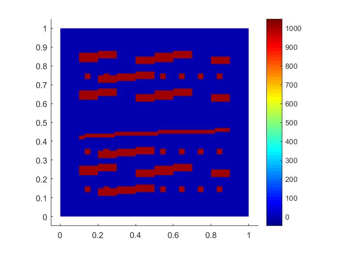
$\kappa$

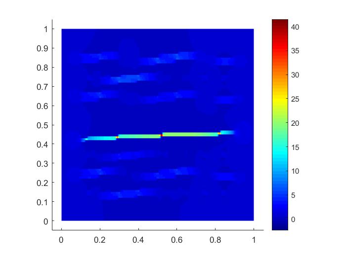
$x$-component of velocity $\bf{v}$

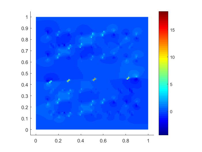
$y$-component of velocity $\bf{v}$

Figure 3: A heterogeneous field $\kappa$ and the corresponding velocity $\bf{v}$.

To compare the accuracy, we will use the following error quantities:

$$e_{1}=\left(\frac{\int_{0}^{T}\int_{\Omega}\left|u_{H}-u_{h}\right|^{2}}{\int_{0}^{T}\int_{\Omega}\left|u_{h}\right|^{2}}\right)^{1/2},\quad\quad e_{2}=\left(\frac{\int_{\Omega}\left|u_{H}(\cdot,T)-u_{h}(\cdot,T)\right|^{2}}{\int_{\Omega}\left|u_{h}(\cdot,T)\right|^{2}}\right)^{1/2}.$$

Furthermore, we introduce the concept of snapshot ratio:

$$\text{snapshot ratio}=\frac{\text{dim}(V_{H}^{(n)})}{\text{dim}(V_{\text{snap}}^{(n)})},$$

where $\text{dim}(V_{H}^{(n)})$ refers to the dimension of offline space, and $\text{dim}(V_{\text{snap}}^{(n)})$ refers to the number of functions $\delta_{ij}(x,t)$ from equation (15).

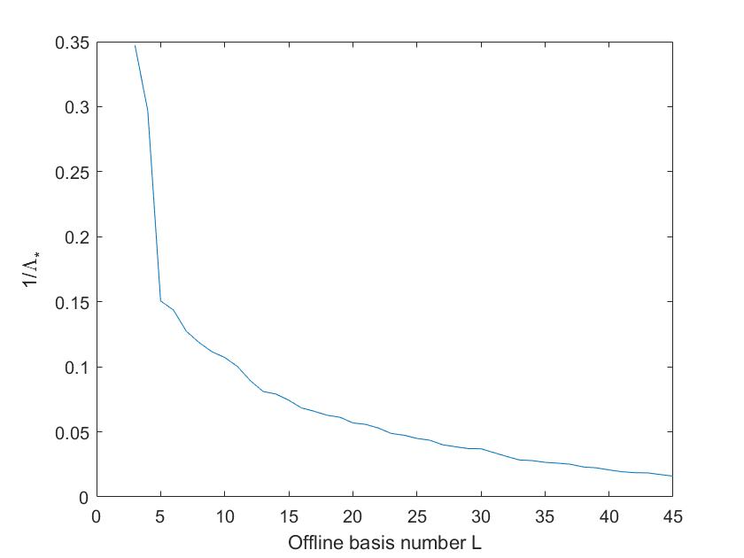
Figure 4: The values $1/\Lambda_{*}$ against number of basis functions.

$L$	dim$(V_{H}^{(n)})$	snapshot ratio	$e_{1}$	$e_{2}$
1	100	0.45%	45.85%	48.38%
3	300	1.34%	7.29%	10.08%
5	500	2.24%	6.01%	8.41%
7	700	3.13%	4.22%	5.73%
10	1000	4.47%	3.48%	4.99%
15	1500	6.71%	2.83%	4.24%
20	2000	8.94%	2.46%	3.64%
25	2500	11.18%	2.07%	3.16%
30	3000	13.41%	1.85%	2.82%

Table 1: Errors for Example 1 (dim$(V_{h}^{(n)})$=72600 and dim$(V_{\text{snap}}^{(n)})$=22365 for each time step $n$).

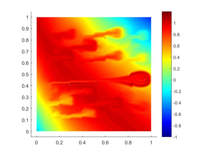
$u_{h}$

$u_{H}\text{ with }L=10$

$u_{H}\text{ with }L=20$

$u_{H}\text{ with }L=30$

Figure 5: $u_{h}$ and $u_{H}$ in Example 1.

In Figure 4, we plot the values $1/\Lambda_{*}$, where $\Lambda_{*}=\min_{K_{i}}\lambda_{L_{i}+1}^{(i)}$, against the number of basis functions. We clearly see the decay of the eigenvalues. We also observe that the decay is much faster for the first few eigenfunctions, which implies that a few basis will give a substantial decay in error. In Table 1, we show the errors using different numbers of offline basis functions $L_{i}$. We see clearly the reduction of error when more basis functions are used, and the reduction of error is more rapid when fewer basis functions are used. We also observe that the method gives reasonable error levels with small snapshot ratios. On the other hand, Figures 5 shows the fine and multiscale solutions at $t=0.08$. From these figures, we observe very good agreements between the fine-scale and multiscale solutions.

In addition, we compare the performance of our method with the use of space-time polynomial basis. For space-time polynomial basis, we build local offline space $V_{H}^{i(n)}$ using $Q_{s}$ functions in $K_{i}\times(T_{n-1},T_{n})$ (total $(s+1)^{3}$ functions), where $s=1,\,2,\,\cdots$ and $Q_{s}$ is the space of polynomials of degree $s$ in each direction. We denote this solution using space-time polynomial basis by $u_{\text{poly}}$. Then, we compare these numerical results to GMsFEM method with $L_{i}=(s+1)^{3}$. In Table 2, we present the errors with the use of $s=1$ and $s=2$ for space-time polynomial basis and the use of $L=8$ and $L=27$ multiscale basis. We note that the dimension of $V_{H}$ is the same for both cases. From this table, we see that the multiscale basis performs better than polynomial basis when the same number of basis is used. Figures 6 shows the corresponding solutions, and we observe that the GMsFEM provides better approximate solutions.

From the results in Tables 1 and 2, we observe our multiscale approach provides an efficient representation of the solution. In particular, if one uses space-time piecewise linear approximation, the errors $e_{1}$ and $e_{2}$ are $6.79\%$ and $9.43\%$ respectively and the dimension of the approximation space for each space-time cell is $8$. On the other hand, the multiscale approach is able to obtain similar error levels by using $3$ multiscale basis functions per space-time cell. Moreover, if one uses space-time piecewise quadratic approximation, the errors $e_{1}$ and $e_{2}$ are $4.12\%$ and $5.36\%$ respectively and the dimension of the approximation space for each space-time cell is $27$. On the other hand, the multiscale approach is able to obtain similar error levels by using $7$ multiscale basis functions per space-time cell.

	$e_{1}$	$e_{2}$
Multiscale basis with $L=8$	4.11%	5.69%
Polynomial basis with $Q_{s}=Q_{1}$	6.79%	9.43%
Multiscale basis with $L=27$	1.95%	2.96%
Polynomial basis with $Q_{s}=Q_{2}$	4.12%	5.36%

Table 2: Comparing the use of multiscale and polynomial basis functions for Example 1.

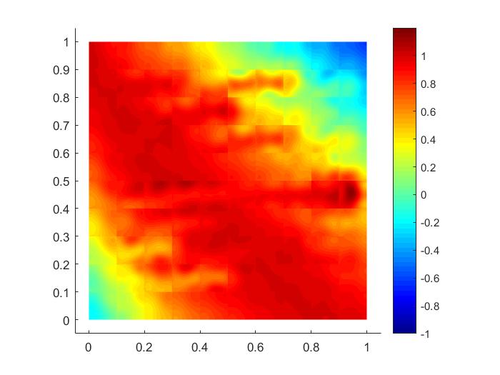
$u_{H}\text{ with }L=8$

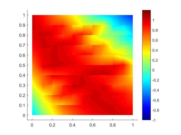
$u_{\text{poly}}\text{ with }Q_{s}=Q_{1}$

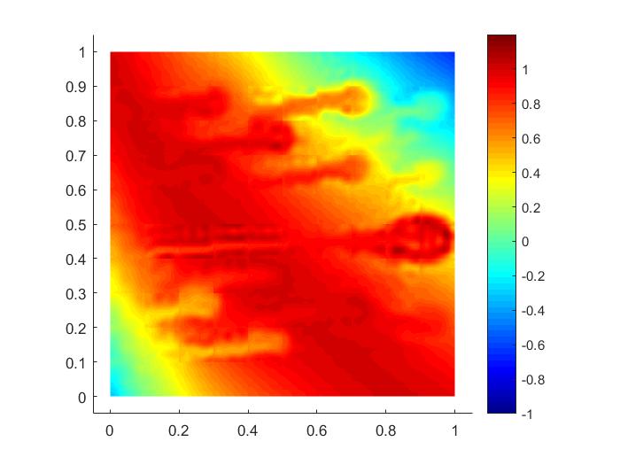
$u_{H}\text{ with }L=27$

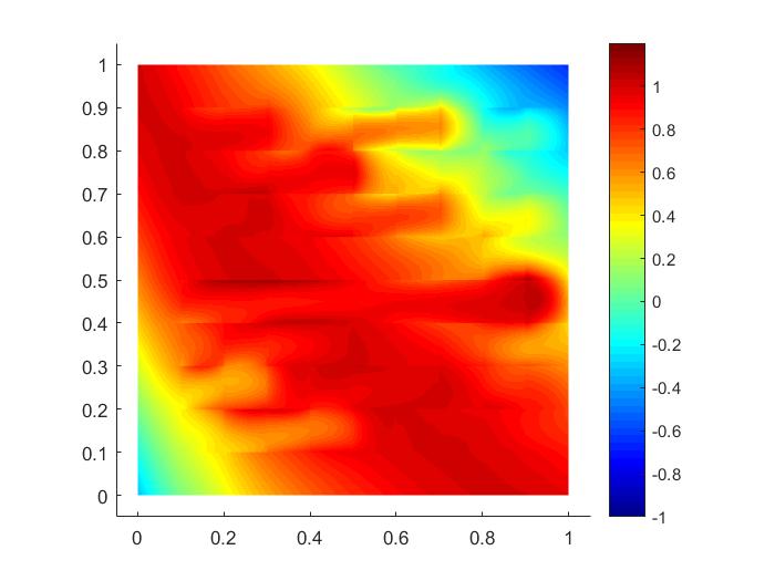
$u_{\text{poly}}\text{ with }Q_{s}=Q_{2}$

Figure 6: Comparing $u_{H}$ with $u_{\text{poly}}$ in Example 1.

4.2 Example 2

In our second example, we also use CG in coarse cell case, take $u_{0}=1-xy$ and $g=1$. The velocity field $\mathbf{v}=(v_{1},v_{2})$ is the same as that in Example 1. In Table 3, we present the errors for using various choices of number of basis functions. We clearly see that, with a very small snapshot ratio, our method is able to obtain solutions with very good accuracy. Furthermore, we observe a faster decay of the error when smaller number of basis functions are used. This confirm the fast decay of eigenvalues in the regime of smaller numbers of basis functions. In Figures 7, we present the fine and multiscale solutions at the time $t=0.08$. We observe very good agreement of both solutions.

$L$	dim$(V_{H}^{(n)})$	snapshot ratio	$e_{1}$	$e_{2}$
1	100	0.45%	44.82%	46.94%
3	300	1.34%	3.96%	5.72%
5	500	2.24%	3.39%	4.92%
7	700	3.13%	2.28%	3.10%
10	1000	4.47%	1.97%	2.74%
15	1500	6.71%	1.43%	2.21%
20	2000	8.94%	1.29%	1.86%
25	2500	11.18%	1.10%	1.65%
30	3000	13.41%	1.02%	1.49%

Table 3: Errors for Example 2 (dim$(V_{h}^{(n)})$=72600 and dim$(V_{\text{snap}}^{(n)})$=22365 for each time step $n$).

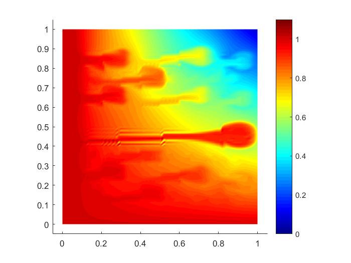
$u_{h}$

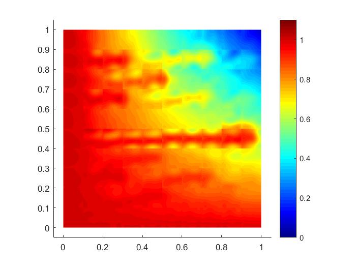
$u_{H}\text{ with }L=10$

$u_{H}\text{ with }L=20$

$u_{H}\text{ with }L=30$

Figure 7: $u_{h}$ and $u_{H}$ in Example 2.

We also compare the performance of our method with the use of space-time polynomial basis functions, and the results are presented in Table 4 and Figures 8. We observe similar conclusions as in the first example. In particular, we see that the multiscale basis functions give more accurate solutions compared with the polynomial basis functions when the same numbers of basis functions are used. We also see from Tables 3 and 4 that multiscale basis functions give faster error decay. For the $e_{1}$ error of about $3.8\%$, our multiscale method needs only $3$ basis functions while the use of polynomial needs $8$ basis functions. Besides, for the $e_{1}$ error of about $2.3\%$, our multiscale method needs only $7$ basis functions while the use of polynomial needs $27$ basis functions. So, we see the rapid decay of error by using multiscale basis functions.

	$e_{1}$	$e_{2}$
Multiscale basis with $L=8$	2.26%	3.11%
Polynomial basis with $Q_{s}=Q_{1}$	3.85%	5.62%
Multiscale basis with $L=27$	1.07%	1.59%
Polynomial basis with $Q_{s}=Q_{2}$	2.46%	3.23%

Table 4: Comparing the use of multiscale and polynomial basis functions for Example 2.

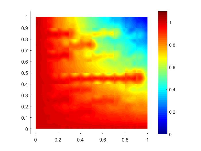
$u_{H}\text{ with }L=8$

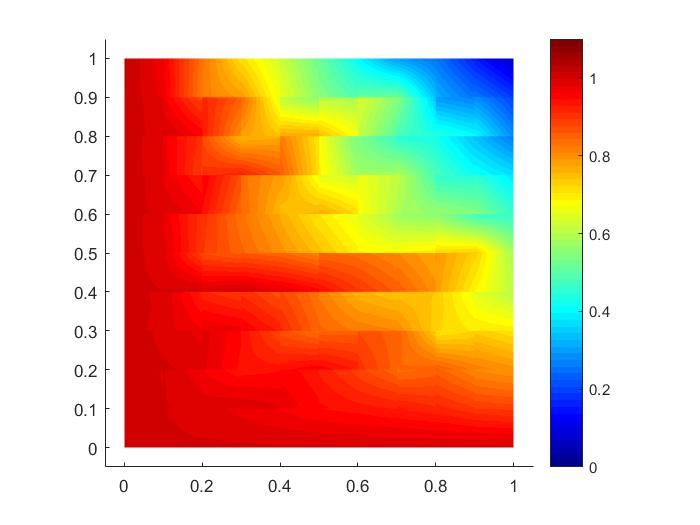
$u_{\text{poly}}\text{ with }Q_{s}=Q_{1}$

$u_{H}\text{ with }L=27$

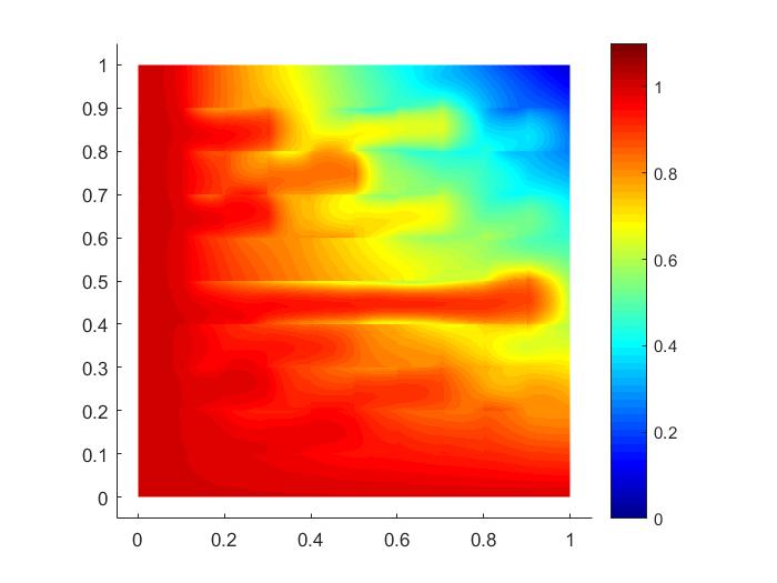
$u_{\text{poly}}\text{ with }Q_{s}=Q_{2}$

Figure 8: Comparing $u_{H}$ with $u_{\text{poly}}$ in Example 2.

5 Conclusion

In this paper, we consider the construction of the space-time GMsFEM to solve time dependent transport equation with heterogeneous velocity field. To our best knowledge, this is a first attempt to generate space-time multiscale basis functions for convection problems, that are known to be challenging because of strong distant effects. Our main objective is to develop systematic multiscale model reduction techniques in space-time cells by constructing local (in space-time) multiscale basis functions. The proposed concepts can be used for other applications, where one needs space-time multiscale basis functions. Our approach focuses on (1) constructing space-time snapshot vectors, (2) performing appropriate t local spectral decomposition in the snapshot space. For snapshot vectors, we solve local problems in local space-time domains. A complete snapshot space includes solutions with all possible boundary and initial conditions. Local spectral decomposition is derived from the analysis. We present a convergence analysis of the proposed method and show that one can obtain a stable and robust multiscale discretization. Several numerical examples are presented. We consider examples where the velocity fields are highly heterogeneous in the space. With only spatial multiscale basis functions are used, we will need a large dimensional space. The space-time multiscale space allows reducing the degrees of freedom. Our numerical results show that one can obtain accurate solutions. Though the presented results are promising, there is a room for further improvements. In particular, we will seek more accurate multiscale basis functions and develop online approaches [13]. The main idea of online approaches is to add multiscale basis functions using the residual information. With appropriate offline spaces, one can achieve a fast convergence with online basis functions. This will be studied in our future work.

6 Acknowledgements

The authors are grateful to Wing Tat Leung for many helpful suggestions.

References

- [1] J.E. Aarnes, Y. Efendiev, and L. Jiang. Analysis of multiscale finite element methods using global information for two-phase flow simulations. SIAM J. Multiscale Modeling and Simulation, 7:2177–2193, 2008.
- [2] T. Arbogast. Analysis of a two-scale, locally conservative subgrid upscaling for elliptic problems. SIAM J. Numer. Anal., 42(2):576–598 (electronic), 2004.
- [3] T. Arbogast and K.J. Boyd. Subgrid upscaling and mixed multiscale finite elements. SIAM J. Numer. Anal., 44(3):1150–1171 (electronic), 2006.
- [4] T. Arbogast, G. Pencheva, M.F. Wheeler, and I. Yotov. A multiscale mortar mixed finite element method. Multiscale Model. Simul., 6(1):319–346 (electronic), 2007.
- [5] T. Arbogast, G. Pencheva, M.F. Wheeler, and I. Yotov. A multiscale mortar mixed finite element method. Multiscale Model. Simul., 6(1):319–346, 2007.
- [6] A. Brandt. Multiscale solvers and systematic upscaling in computational physics. Computer Physics Communication, 169:438–441, 2005.
- [7] Fuchen Chen, Eric Chung, and Lijian Jiang. Least-squares mixed generalized multiscale finite element method. Computer Methods in Applied Mechanics and Engineering, 311:764–787, 2016.
- [8] Y. Chen, L. Durlofsky, M. Gerritsen, and X. Wen. A coupled local-global upscaling approach for simulating flow in highly heterogeneous formations. Advances in Water Resources, 26:1041–1060, 2003.
- [9] C.-C. Chu, I. G. Graham, and T.-Y. Hou. A new multiscale finite element method for high-contrast elliptic interface problems. Math. Comp., 79(272):1915–1955, 2010.
- [10] E. Chung, Y. Efendiev, and C. Lee. Mixed generalized multiscale finite element methods and applications. SIAM Multicale Model. Simul., 13:338–366, 2014.
- [11] E. T. Chung, Y. Efendiev, and G. Li. An adaptive GMsFEM for high contrast flow problems. J. Comput. Phys., 273:54–76, 2014.
- [12] Eric Chung, Yalchin Efendiev, and Thomas Y Hou. Adaptive multiscale model reduction with generalized multiscale finite element methods. Journal of Computational Physics, 320:69–95, 2016.
- [13] Eric T Chung, Yalchin Efendiev, and Wing Tat Leung. Residual-driven online generalized multiscale finite element methods. Journal of Computational Physics, 302:176–190, 2015.
- [14] Eric T Chung, Yalchin Efendiev, Wing Tat Leung, and Shuai Ye. Generalized multiscale finite element methods for space-time heterogeneous parabolic equations. arXiv preprint arXiv:1605.07634, 2016.
- [15] Eric T Chung, Maria Vasilyeva, and Yating Wang. A conservative local multiscale model reduction technique for stokes flows in heterogeneous perforated domains. Journal of Computational and Applied Mathematics, 2017.
- [16] Y. Efendiev and J. Galvis. Domain decomposition preconditioner for multiscale high-contrast problems. In Proceedings of DD19, 2009.
- [17] Y. Efendiev and J. Galvis. Eigenfunctions and multiscale methods for Darcy problems. Technical report, ISC, Texas A& M University, 2010.
- [18] Y. Efendiev, J. Galvis, and T. Hou. Generalized multiscale finite element methods. Journal of Computational Physics, 251:116–135, 2013.
- [19] Y. Efendiev, J. Galvis, S. Ki Kang, and R.D. Lazarov. Robust multiscale iterative solvers for nonlinear flows in highly heterogeneous media. Numer. Math. Theory Methods Appl., 5(3):359–383, 2012.
- [20] R. Ewing, O. Iliev, R. Lazarov, I. Rybak, and J. Willems. A simplified method for upscaling composite materials with high contrast of the conductivity. SIAM J. Sci. Comput., 31(4):2568–2586, 2009.
- [21] Thomas Y Hou and Xue Xin. Homogenization of linear transport equations with oscillatory vector fields. SIAM Journal on Applied Mathematics, 52(1):34–45, 1992.
- [22] O Iliev, Z Lakdawala, and V Starikovicius. On a numerical subgrid upscaling algorithm for stokes–brinkman equations. Computers & Mathematics with Applications, 65(3):435–448, 2013.
- [23] O. Iliev, R. Lazarov, and J. Willems. Fast numerical upscaling of heat equation for fibrous materials. Comput. Vis. Sci., 13(6):275–285, 2010.
- [24] O. Iliev, R. Lazarov, and J. Willems. Variational multiscale finite element method for flows in highly porous media. Multiscale Model. Simul., 9(4):1350–1372, 2011.
- [25] O.P. Iliev, I. Rybak, and J. Willems. On upscaling of heat conductivity for a class of industrial problems. J. Theoretical and Applied Mechanics. submitted.
- [26] Béatrice Rivière. Discontinuous Galerkin methods for solving elliptic and parabolic equations: theory and implementation. Society for Industrial and Applied Mathematics, 2008.
- [27] P.S. Vassilevski. Coarse spaces by algebraic multigrid: multigrid convergence and upscaling error estimates. Adv. Adapt. Data Anal., 3(1-2):229–249, 2011.
- [28] E Weinan. Homogenization of linear and nonlinear transport equations. Communications on Pure and Applied Mathematics, 45(3):301–326, 1992.
- [29] X.H. Wu, Y. Efendiev, and T.Y. Hou. Analysis of upscaling absolute permeability. Discrete and Continuous Dynamical Systems, Series B., 2:158–204, 2002.