Off the Beaten Track: Using Deep Learning to Interpolate Between Music Genres

Abstract

We describe a system based on deep learning that generates drum patterns in the electronic dance music domain. Experimental results reveal that generated patterns can be employed to produce musically sound and creative transitions between different genres, and that the process of generation is of interest to practitioners in the field.

Automatic music generation is a fast growing area with applications in diverse domains such as gaming [1], virtual environments [2], and entertainment industry [3]. A thorough account of goals and techniques is presented in [4]. Electronic dance music (EDM) is one of the domains where automatic generation appears to be particularly promising due to its heavily constrained repetitive structure, characterized by clearly defined stylistic forms [5]. In this domain, a typical task of “traditional” Disk-Jockeys (DJs) operating in dance clubs and radio stations is to obtain seamless transitions between the consecutive tracks of a given playlist. When the individual song tracks are entirely pre-recorded, the main tools available to DJs are a combination of an accurate synchronization of beats-per-minute (BPM) via beatmatching, and a perceptually smooth crossfading (i.e.  gradually lowering the volume of one track while increasing the volume of the other track), occasionally with the help of equalizers and other effects such as reverbs, phasers, or delays, which are commonly available in commercial mixing consoles. However, since the early 1990’s, it has become increasingly common for DJs to take advantage of samplers and synthesizers that can be used to generate (compose) on-the-fly novel musical parts to be combined with the existing pre-recorded material. Artists such as DJ Shadow and DJ Spooky have indeed demonstrated that the line demarcating DJing and electronic music composition can be extremely blurry [6].

In this paper, we explore the automation of track transitioning when the consecutive tracks belong to different genres. Previous attempts to automate track transitioning are limited to time-stretching and crossfading [7], essentially mimicking the human work of a traditional DJ. While these approaches can effectively achieve the goal of a seamless mix between pre-recorded tracks (particularly when the tracks stay within the same musical genre), they hardly fit the contemporary scenario where DJs and composers are seeking artistically interesting results also by using in a creative way transitions spanning different genres. We thus advocate a radically different perspective where novel musical material is automatically generated (composed) by the computer in order to smoothly transition from one genre to another. The hope is that by exploring this smooth musical space in an automatic fashion, we can create materials that are useful to musicians as novel elements in composition and performance. In this new approach, we thus take transitions be compositional devices in their own right. Depending on length, transitions serve different functions in dance music: they could be momentary sound effects on a short time scale, or comparable to frequency sweeps on longer time scales, or on even longer scales to act as an automatically generated foundation on top of which musical layers can be added, both in live performance and post-production.

Building a general interpolation tool that encompasses the whole set of instruments is beyond the scope of this paper. Genre in the domain of EDM is mainly determined by the basic rhythm structure of drum instruments. Hence, by taking these drum patterns as the musical material for an experiment, the complexity associated with other aspects such as harmony, melody and timbre [8], that are relevant for genre in other musical domains, can be sidestepped. At the same time, the domain remains sufficiently complex and suitable for significant real-world usage by music professionals such as DJs, producers, and electronic musicians.

To investigate the potential of deep learning for transitioning between dance music genres, we designed a learning system based on variational autoencoders [9], we trained it on a dataset of rhythm patters from different genres that we created, and then we asked it to produce interpolations between two given rhythm patterns. Such transitions consist of a sequence of rhythm patterns, starting from a given pattern from one genre and ending in a given goal pattern (possibly from another genre). The connecting patterns in between are new rhythm patterns generated by the trained system itself. Along the same vein, we also developed an autonomous drummer that smoothly explores the EDM drum pattern space by moving in the noise space of a generative adversarial network [10]. We constructed an experimental software instrument that allows practitioners to create interpolations, by embedding the learning system in Ableton Live, a music software tool commonly used within the EDM production community. Finally, the proposed process for creating interpolations and the resulting musical materials were thoroughly evaluated by a set of musicians especially recruited for this research.

Generative Machine Learning

Many machine learning applications are concerned with pattern recognition problems in the supervised setting. Recently, however, a rather different set of problems has received significant attention, where the goal is to generate patterns rather than recognize them. Application domains are numerous and diverse and very often involve the generation of data for multimedia environments. Examples include natural images [11], videos [12], paintings [13], text [14], and music [15, 14, 8].

Pattern generation is closely related to unsupervised learning, where a dataset $\{x^{(1)},\dots,x^{(n)}\}$ of patterns, sampled from an unknown distribution $p$, is given as input to a learning algorithm whose task is to estimate $p$ or to extract useful information about the structure of $p$ such as clusters (i.e.  groups of similar patterns) or support (i.e.  regions of high density, especially when it consists of a low-dimensional manifold). In pattern generation, however, we are specifically interested in sampling new patterns from a distribution that matches $p$ as well as possible. Two important techniques for pattern generation are generative adversarial networks and (variational) autoencoders, briefly reviewed in the following.

Generative Adversarial Networks

Generative Adversarial Networks (GANs) [10] consist of a pair of neural networks: a generator, $\mathcal{G}:\mathds{R}^{d}\mapsto\mathds{R}^{m}$, parameterized by weights $w_{g}$, and a discriminator, $\mathcal{D}:\mathds{R}^{m}\mapsto\{0,1\}$, parameterized by weights $w_{d}$. The generator receives as input a vector $z\in\mathds{R}^{d}$ sampled from a given distribution $q$ and outputs a corresponding pattern $\mathcal{G}(z)\in\mathds{R}^{m}$. We can interpret $z$ as a low-dimensional code for the generated pattern, or as a tuple of coordinates within the manifold of patterns. The discriminator is a binary classifier, trained to separate true patterns belonging to the training dataset (positive examples) from fake patterns produced by the generator (negative examples). Training a GAN is based on an adversarial game where the generator tries to produce fake patterns that are as hard to distinguish from true patterns as possible, while the discriminator tries to detect fake patterns with the highest possible accuracy. At the end of training we hope to reach a game equilibrium where the generator produces realistic patterns as desired. The discriminator is no longer useful after training. Equilibrium is sought by minimizing the following objective functions, for the discriminator and for the generator, respectively:

$$J_{d}(w_{d}) = \mathbb{E}_{x\sim p}\left[L(\mathcal{D}(x),1)\right]+\mathbb{E}_{z\sim q}\left[L(\mathcal{D}(\mathcal{G}(z)),0)\right]$$ (1)

$$J_{g}(w_{g}) = \mathbb{E}_{z\sim q}\left[L(\mathcal{D}(\mathcal{G}(z)),1)\right]$$ (2)

where $L$ denotes the binary cross-entropy loss, $q$ can be either a uniform distribution on a compact subset of $\mathds{R}^{d}$ or, alternatively, a Gaussian distribution with zero mean and unit variance. Since $p$ is not accessible, the expectation in Eq. (1) is replaced by its empirical value on the training sample. In practice, fake data points are also sampled. Optimization typically proceeds by stochastic gradient descent or related algorithms where a balanced minibatch of real and fake examples is generated at each optimization step.

Autoencoders and Variational Autoencoders

Autoencoders also consist of a pair of networks: an encoder, $\mathcal{E}$, parameterized by weights $w_{e}$, that maps an input pattern $x\in\mathds{R}^{m}$ into a latent code vector $z=\mathcal{E}(x)\in\mathds{R}^{d}$, and a decoder, $\mathcal{D}$, parameterized by weights $w_{d}$, mapping latent vectors $z\in\mathds{R}^{d}$ back to the pattern space $\mathds{R}^{m}$. In this case, the two networks are stacked one on the top of the other to create a composite function $\mathcal{D}\circ\mathcal{E}:\mathds{R}^{m}\mapsto\mathds{R}^{m}$, and the overall model is trained to reproduce its own inputs at the output. Since typically $d\ll m$, the model is forced to develop a low-dimensional representation that captures the manifold of the pattern associated with the data distribution $p$. Training is performed by minimizing the objective

$$J(w_{e},w_{d}) = \mathbb{E}_{x\sim p}\left[L(\mathcal{D}(\mathcal{E}(x)),x)\right]$$ (3)

where the parameters $w_{e}$ and $w_{d}$ are optimized jointly and $L$ an appropriate reconstruction loss.

Variational autoencoders (VAEs) [9] also consist of an encoder and a decoder, but they bear a probabilistic interpretation. To generate a pattern, we first sample a vector $z\in\mathds{R}^{d}$ from a prior distribution $p(z)$ (usually a multivariate Gaussian with zero mean and unit variance), and we then apply $z$ as input to the decoder, in order to obtain $p(x|z)$. The encoder in this case produces an approximation $q(z|x)$ to the intractable posterior $p(z|x)$. Specifically, $q(z|x)$ is a multivariate Gaussian whose mean $\mu(x)$ and diagonal covariance $\sigma(x)$ are computed by the encoder network $\mathcal{E}$ receiving a pattern $x$ as input. A VAE is then trained to minimize the difference between the Kullback-Leibler divergence

$$\mathrm{KL}(q(z)||p(z)) = \int q(z)\log\frac{p(z)}{q(z)}dz$$

$$= \frac{1}{2}\sum_{j=1}^{d}\left(1+\log\sigma^{2}_{j}(x)-\mu^{2}_{j}(x)-\sigma^{2}_{j}(x)\right)$$

and the log conditional likelihood

$$\log p(x|z)=-\mathbb{E}_{x\sim p}\left[L(x,\mathcal{D}(z))\right].$$ (5)

Deep and Recurrent Networks

All the above networks (generator and discriminator for GANs, decoder and encoder for VAEs) can be constructed by stacking several neural network layers. In particular, our encoder for the VAE was based on three bidirectional long-short-term-memory (LSTM) [16] recurrent layers with tanh nonlinearities, followed by four fully connected layers with ReLU nonlinearities, ending in a representation of size $d=4$. LSTM layers were used to capture the temporal structure of the data and, in particular, the correlations among note-on MIDI events within a drum pattern. Convolutional layers could have also been employed and we found that they produce similar reconstruction errors during training. We developed a slight aesthetic preference towards LSTM layers in our preliminary listening sessions during the development of the VAE, although differences compared to convolutional layers were not very strong. The decoder simply consisted of five fully connected layers with ReLUs. We used logistic units on the last layer of the decoder and a binary cross-entropy loss for comparing reconstructions against true patterns, where MIDI velocities were converted into probabilities by normalizing them in [0,1]. Details on the architecture are visible in Figure 1.

The discriminator and the generator networks for the GAN had essentially the same architectures as the encoder and the decoder for the VAE, respectively, except of course the GAN discriminator terminates with a single logistic unit and for the VAE we used a slightly smaller (two-dimensional) noise space, in order to exploit the “swirling” explorer described below in the “autonomous drumming” subsection.

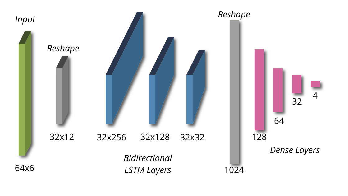
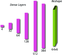
Figure 1: Architecture of the variational autoencoder used to interpolate drum patterns. Top: Encoder; Bottom: Decoder.

Electronic Dance Music Dataset

One of the authors, who is a professional musician, used his in-depth knowledge of EDM to compose a collection of drum patterns representative of three genres: Electro, Techno, and Intelligent Dance Music (IDM). In all patterns, the following six instruments of a Roland TR-808 Rhythm composer drum machine were used: bass drum, snare drum, closed hi-hat, open hi-hat, rimshot, and cowbell. The TR-808 (together with its sisters TR-606 and TR-909), was integral to the development of electronic dance music and these six instrument sounds are still widely used in EDM genres today which makes them suitable for our interpolation approach. All patterns are one measure (4 bars) long, and quantized to 1/16th note on the temporal scale. At the intended tempo of 129 BPM, it takes 7.44s to play one measure. Patterns were constructed with the help of the Ableton Live music production software, and delivered in the form of standard MIDI files. After checking for duplicates, a data set consisting of 1782 patterns resulted, which is summarized in Table I.

Each drum pattern was represented as a two-dimensional array whose first and second axes are associated with the six selected drum instruments and the temporal position at which a MIDI note-on event occurs, respectively. Note durations were not included in the representation as they are irrelevant for our choice of percussive instruments. The duration of four measures results in a $6\times 64$ array for each pattern. Values (originally in the integer range [0,127], then normalized in [0,1]) correspond to MIDI velocities and were used during dataset construction mainly to represent dynamic accents or ghost (echoing) notes that may be present in some musical styles. In our representation, a zero entry in the array indicates the absence of a note-on event.

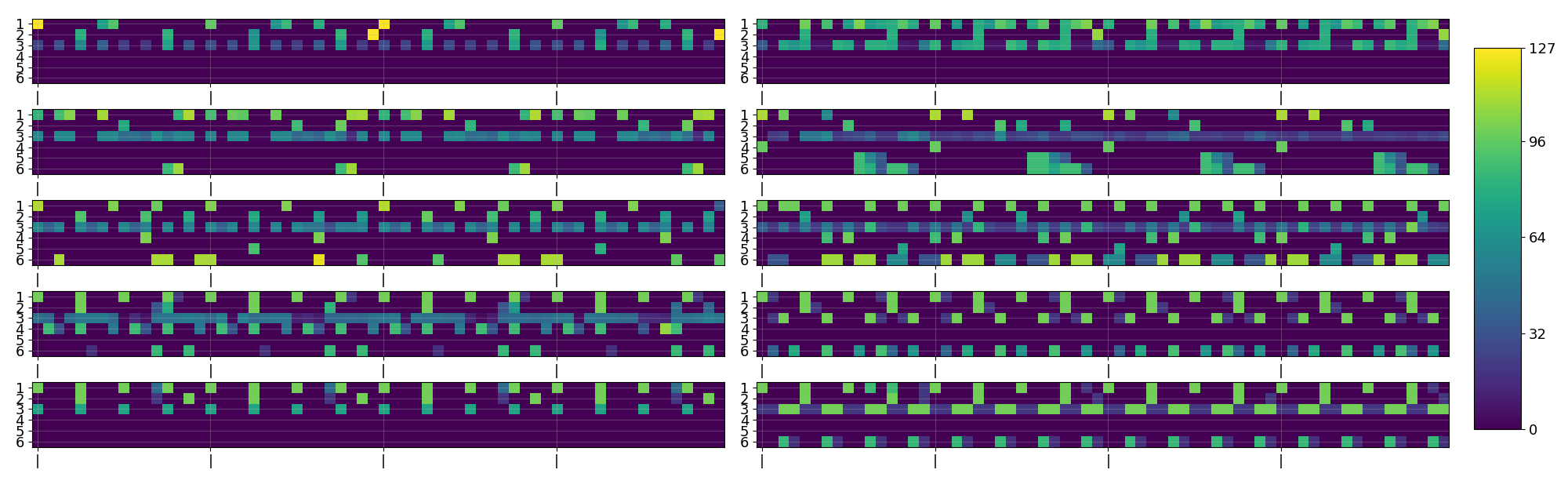
Figure 2: Ten sample drum patterns in the EDM dataset. Instruments from the top are (1): bass drum, (2): snare drum, (3): closed hi-hat, (4): open hi-hat, (5): rimshot, (6): cowbell. Pixel intensities correspond to MIDI velocities. Top row: Electro-Funk; mid two rows: IDM; bottom two rows: Techno.

TABLE I: Electronic Dance Music Dataset

Style	# of patterns	Playing time
IDM	$608$	$4$,525s	(1h 15m 25s)
Electro	$690$	$5$,135s	(1h 25m 35s)
Techno	$484$	$3$,602s	(1h 0m 2s)
Total	$1$,782	$13$,261s	(3h 41m 1s)

Generating interpolations

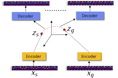
Figure 3: Building transitions by interpolating drum patterns in their representation space.

Both techniques discussed above were used to generate sequences of drum patterns that interpolate between genres.

Using VAEs for start-goal interpolations

When using VAEs, it is straightforward to create an interpolation between a starting pattern $x_{s}$ and a goal pattern $x_{g}$ as follows (see also Figure 3):

1. Apply the encoder $\mathcal{E}$ to the endpoint patterns to obtain the associated coordinates in the manifold space of the autoencoder: $z_{s}=\mathcal{E}(x_{s})$ and $z_{g}=\mathcal{E}(x_{g})$;

2. For a given interpolation length, $L$, construct a sequence of codes in the manifold space: $\langle z_{0}=z_{s},z_{1},\dots,z_{L}=z_{g}\rangle$

3. Apply the decoder $\mathcal{D}$ to each element of this sequence, to obtain a sequence of patterns: $\langle\mathcal{D}(z_{0}),\dots,\mathcal{D}(z_{L})\rangle$; note that (unless the autoencoder underfits the dataset) $\mathcal{D}(z_{0})\approx x_{s}$ and $\mathcal{D}(z_{L})\approx x_{g}$.

Linear and spherical interpolation

In the case of linear interpolation (LERP), the sequence of codes is defined as

$$z_{i}=(1-\mu_{i})z_{s}+\mu_{i}z_{g}$$ (6)

for $\mu_{i}=i/L$, $i=0,\dots L$. In the case of spherical interpolation (SLERP), the sequence is

$$z_{i}=\frac{z_{s}\sin(\theta(1.0-\mu_{i}))+z_{g}\sin(\theta\mu_{i})}{\sin(\theta)}$$ (7)

where $\theta=\arccos(\frac{h^{\intercal}_{s}z_{g}}{\|z_{s}\|\|z_{g}\|})$. [17] offers a thorough discussion of the benefits of SLERP in the case of image generation. We found that SLERP interpolations produced musically more adventurous and expressive results and thus we used them in our experimental evaluation.

Crossfading vs. interpolation in the representation space

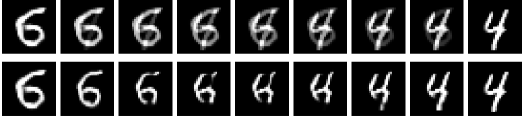
Figure 4: Top: Interpolation in the pattern space (i.e., crossfading) between two MNIST characters; Bottom: interpolation in the representation space.

We remark the significance of performing the interpolation in the representation space: rather than generating a weighted average of two patterns (as it would happen with crossfading, which consists of a linear combination as in Eq. 6 but using identity functions instead of $\mathcal{E}$ and $\mathcal{D}$), we generate at each step $i$ a novel drum pattern from the learned distribution. To help the reader with a visual analogy, we show in Figure 4 the difference between interpolation in pattern space (crossfading) and in representation space using two handwritten characters from the MNIST dataset.

Pattern novelty

A quantitative measure of quality and novelty of patterns generated by models such as VAEs or GANs is not readily available. We observed however that several of the patterns produced by interpolating between start and goal patterns in our dataset are genuinely new. In Figure 5 we visualize the result of two-dimensional principal components analysis (PCA) showing all training set patterns and those generated by interpolating between a subset of them. It can be seen that trajectories tend to respect the distribution of the training data but include new data points, showing that novel patterns are indeed generated in the transitions.

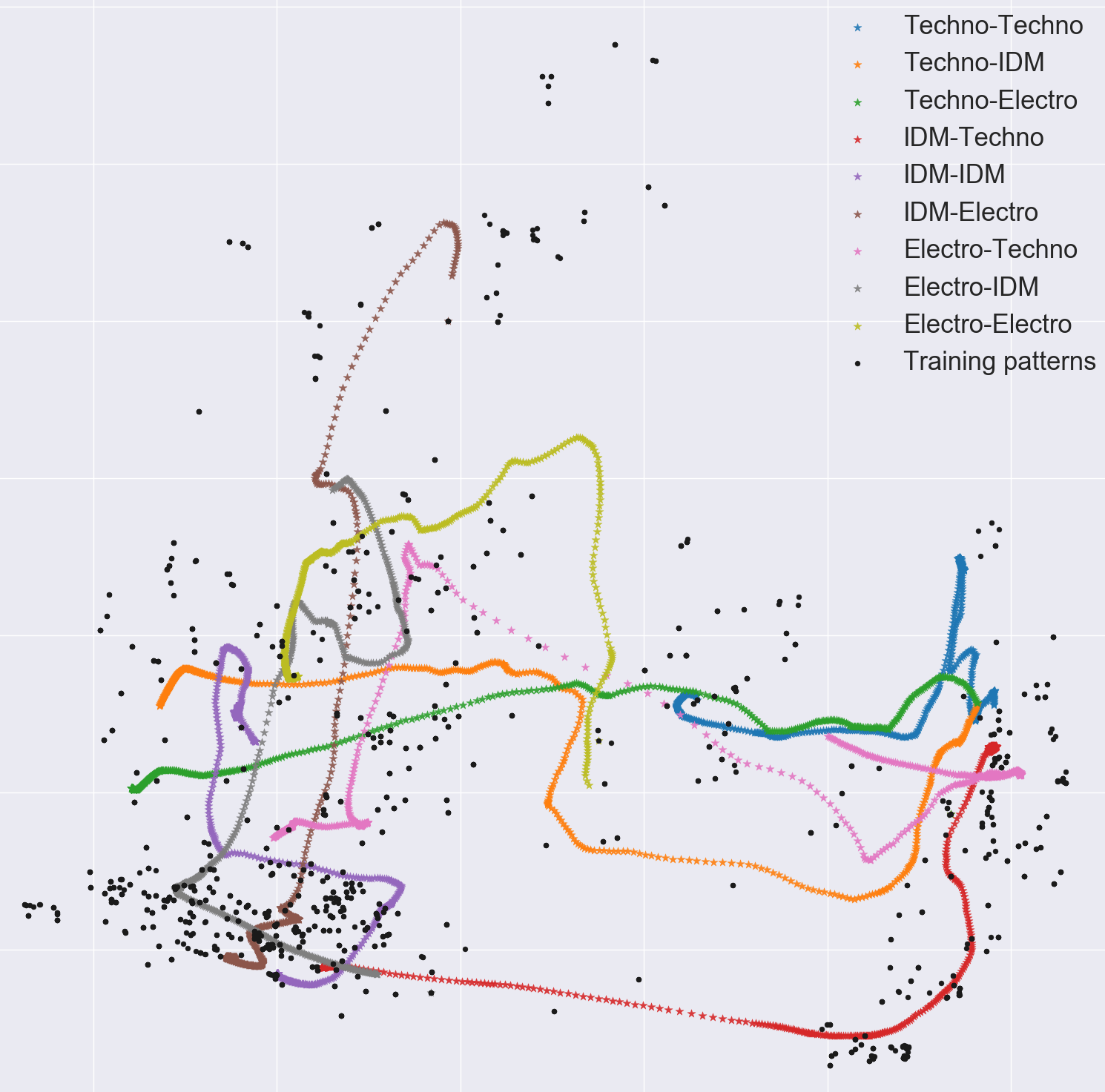
Figure 5: PCA plot of training data (black dots) and a set of possible start-goal interpolations obtained with a deep LSTM VAE (labeled by the genres of the start and goal patterns).

A software instrument for start-goal interpolations

The trained VAE (in the form of a Tensorflow model) was embedded as a plugin in Ableton Live Suite 9 for Mac OS, a program that is widely used by performing and producing musicians in EDM, and that enables the construction of software instruments via the programming environment Max for Live. During performance, musicians first specify a start and a goal pattern (chosen from the dataset), and the length of the interpolation. This can be conveniently done within the Live user interface. The controller (a small Python script) then produces the required sequence of patterns using the VAE and the resulting MIDI notes are sent to Live to be rendered in audio with a user-specified soundset. The whole process is fast enough for real-time usage.

Using GANs for autonomous drumming

In the case of GANs, Step 1 of the procedure we used to create start-goal interpolations with VAEs is not readily available. We attempted to “invert” the generator network using the procedure suggested in [18] but our success was limited since training patters are largely not reproducible by the generator. Although unsuitable for start-goal interpolations, we found that GANS are very effective to create an autonomous drummer by exploring the noise space in a smooth way. Exploration can be designed in many ways and here we propose a very simple approach based on the following complex periodic function

$$f(t,\omega_{1},\omega_{2},\omega_{3},\omega_{4})\doteq e^{\omega_{1}jt}-\frac{e^{\omega_{2}jt}}{2}+\frac{je^{\omega_{3}jt}}{3}+\frac{e^{\omega_{4}jt}}{4}$$ (8)

for $t\in[0,2\pi]$ and constants $\omega_{1}=2$, $\omega_{2}=19$, $\omega_{3}=-20$, $\omega_{4}=20$. Using a GAN with $d=2$, the real and the imaginary part of $f$ are used to form the two components of vector $z$. The resulting “swirl” in noise space is illustrated in Figure 6.

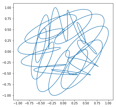
Figure 6: Swirl in GAN noise space associated with Eq. 8.

Evaluation experiments

Although patterns generated by VAEs and GANs are novel, we still need to establish that they do add something new to the current practice of EDM and that they are of interest to its practitioners. To this end, we designed three experiments where we asked professional musicians to assess the quality of the generated patterns. The identification experiment aims to verify if practitioners are able to tell start-goal interpolations apart from start-goal crossfades; the task experiment aims to assess how much musicians appreciated and were able to make use of the drum interpolation as a compositional tool; the robot experiment aims to rate the aesthetic quality of the autonomous drumming produced by the GAN when generating patterns by swirling in the representation space. The goal was to answer the following questions:

Q1: Are musicians able to tell interpolations and crossfades between genres apart during listening sessions?

Q2: How do practitioners rate the novelty, adequacy, and style of the “instrument” for creating interpolations between genres?

Q3: Are the drum tracks generated by moving or interpolating smoothly in the representation space of VAEs and GANs useful as a material for musicians in composition and performance?

Identification experiment

The goal of the experiment was to answer Q1. Subjects were asked to listen to pairs of transitions, a crossfade and an interpolation. Both straight and mixed pairs were formed, in which starting and goal patterns were identical or different, respectively. Three drum patterns for each of the three genres were chosen from the dataset. Nine different transitions using these patterns were specified in a design that includes a transition for each possible pair of genres in both directions, as well a transition within each of the three genres. Interpolations and crossfades had a length of 6 measures (24 bars, 44.7s playing time). For interpolations, the endpoints were the VAE’s reconstructions of the start and goal pattern. Crossfades were produced using a standard function (equal power) of Logic Pro X.

The difference between an interpolation and a crossfade was explained to the subjects in the visual domain using an animated version of Figure 4. Every subject was asked to tell apart 6 pairs, preceded by one practice pair to get acquainted with the procedure, and received no feedback on the correctness of their answers.

Task experiment

The goal of the experiment was to answer Q2 and Q3. We used the creative product analysis model (CPAM) [19], that focuses on the following three factors: Novelty, Resolution, and Style. Each factor is characterized by a number of facets that further describe the product. For each facet, there is a 7-point scale built on a semantic differential: subjects are asked to indicate their position on the scale between two bipolar words (also referred to as anchors). Novelty involves two facets: Originality and Surprise. Resolution considers how well the product does what it is supposed to do and has four facets: Logicality, Usefulness, Value, and Understandability. Style considers how well the product presents itself to the customer and has three facets: Organicness, Well- craftedness, and Elegance. In this experiment, subjects were allowed to choose start and goal patterns from those available in the dataset in order to create their own interpolations using our Ableton Live interface. In this experiment, subjects were allowed to choose start and goal patterns from those available in the dataset in order to create their own interpolations using our Ableton Live interface.

Robot experiment

The goal of the experiment was to answer Q3. We used in this case the Godspeed questionnaire [20] a well-known set of instruments designed to measure the perceived quality of robots, based on subjects’ observations of a robot’s behavior in a social setting. They consist of 5-point scales based on semantic differentials. In our case, observation is limited to hearing the artificial agent drum and thus we chose to measure only two factors: Animacy (three facets: Lively, Organic, Lifelike) and Perceived Intelligence (three facets: Competent, Knowledgeable, Intelligent).

A long interpolation of 512 bars (124 measures) was generated using the trained GAN, by “sweeping” the code space with a complex function. Six segments of 60 bars each were selected from the MIDI file, 9 measures preceded and followed by half a measure (2 bars) for leading in and out. These MIDI files were rendered into sound using an acoustic drum soundset in Logic Pro X (Drum Designer/Smash kit), where the parts of the rimshot and cowbell were transposed to be played by toms. Acoustic rather than electronic drum sounds were used to facilitate the comparison with human drumming. Subjects were instructed that they were going to listen to an improvisation by an algorithmic drummer, presented with one of the 6 audio files (distributed evenly over the subject population), and asked to express a judgment on animacy and perceived intelligence.

Experimental procedure

The experiments were conducted with subjects active in the wider field of electronic music (DJs, producers, instrumentalists, composers, sound engineers), that were familiar with the relevant genres of EDM. Their experience in electronic music ranged from 2–30 years (median 7 years, average 8.75). They were recruited by the authors from educational institutes and the local music scenes in Krakow (PL), Cuneo and the wider Firenze area (IT), and Eindhoven (NL). Experiments took place in a class room or music studio setting, where subjects listened through quality headphones or studio monitors. All audio materials in the experiment were prepared as standard stereo files (44.1 kHz, 16 bits).

(a)	(b)

Figure 7: (a): Task experiment box plots (n=16, 7-point scale); (b): Robot experiment box plots (n= 38, 5-point scale).

Results

We now present and discuss the experimental results.

Identification experiment

This experiment was conducted with 19 subjects using 18 distinct stimulus pairs. 13 identification errors were made in 114 pairs. For each pair correctly identified by a subject 1 point was awarded (0 for a miss). Subjects achieved an average score of $2.68\pm 0.8$ and $2.63\pm 0.58$ (out of 3) for straight and mixed interpolations, respectively. In total they achieved a score of $5.32\pm 1.03$ (out of 6). A Chi-squared test confirms that participants scored better than chance $\chi^{2}(19)=25.92$ (critical value $5.99$). Clearly, subjects are able to tell interpolations and crossfades apart in a musical context.

Task experiment

Fifteen subjects with knowledge of the means of EDM production were invited to construct an interpolation with the Ableton Live interface as described above (six of them had previously participated in the Identification experiment). We asked them to rate their experience (process and result) on the CPAM scales. Figure 7(a) summarizes the results in a set of box plots, one for each of the facets. Median scores for all facets are 6 (for Value even 7). The average scores for the facets of the factor Resolution (Logicality 6; Usefulness 6.13; Value 6.5; Understandability 5.8) are generally slightly higher than those for the factors Novelty (Originality 6.13; Surprise 5.94) and Style (Organic 5.82; Well-craftedness 6.06; Elegant 5.88). Although we did not use the CPAM to compare different solutions for generating transitions between drum tracks, subjects judged the process for creating interpolations and its results against their background knowledge of existing techniques such as crossfades. The relatively high scores on all facets indicate that developing the current prototype into an interpolation instrument will be of value to practitioners in the field.

Robot experiment

We asked 38 subjects to listen to a drum track produced by the trained GAN and to rate the robotic drummer on the scales for Animacy and Perceived Intelligence. Figure 7(b) summarizes the result in a set of box plots for the aspects. The median score on all aspects is 4, with the exception of Lifelike where it is 3. Average scores are higher for the aspects of Perceived Intelligence (Competent 4.24; Knowledgeable 3.95; Intelligence 3.84) than for those of Animacy (Lively 3.89; Organic 3.45; Lifelike 3.13). Comments written by the subjects indicate that they judged Perceived Intelligence mainly with respect to the construction and evolution of the patterns, whereas for Animacy the execution of the patterns was more prominent: absence of small variations in timing and timbre of the drum hits pushed their judgments towards the anchors Stagnant, Mechanical, and Artificial. This could be addressed with standard techniques to “humanize” sequenced drum patterns by slightly randomizing the note onsets and velocities, and rotating between multiple samples for each of the instruments, but for this experiment we used the patterns output by the GAN without such alterations. Even though this measurement just sets a first benchmark for further development, the high scores for Competent and Knowledgeable are encouraging as they suggest that the deep learning process has captured the genres in the dataset to a large extent.

Conclusion

Our tool has already potential applications. First, it can be used to improve the process of producing (and delivering) libraries of drum patterns as the trained network can generate a large number of patterns in the style represented by the training data. Second, it can support the workflows of dance musicians in new ways. Generated interpolation tracks can be recorded inside the tool to create fragments to be used in post-production or during live performance as a foundation on which a DJ or instrumentalist can layer further musical elements. In addition, VAEs or GANs can be trained on materials created by individual users, providing users with a highly customized software instrument that “knows” their personal style and is able to generate new drum tracks in this style for post-production or in performance.

There are several directions that can be followed to further enrich the drumming space, including the generation of tempo for tracks that require tempo that varies over time, and the generation of additional information for selecting drum sounds in a wide soundset. A more ambitious direction is to extend our approach for generating whole sets of instruments (bass lines, leads, pads, etc.) in EDM, which involves not only note onsets but also pitch and duration.

References

- [1] D. Plans and D. Morelli, “Experience-driven procedural music generation for games,” IEEE Transactions on Computational Intelligence and AI in Games, vol. 4, no. 3, pp. 192–198, 2012.
- [2] P. Casella and A. Paiva, “Magenta: An architecture for real time automatic composition of background music,” in Intelligent Virtual Agents. Springer, 2001, pp. 224–232.
- [3] J.-I. Nakamura, T. Kaku, K. Hyun, T. Noma, and S. Yoshida, “Automatic background music generation based on actors’ mood and motions,” The Journal of Visualization and Computer Animation, vol. 5, no. 4, pp. 247–264, Oct. 1994.
- [4] P. Pasquier, A. Eigenfeldt, O. Bown, and S. Dubnov, “An Introduction to Musical Metacreation,” Computers in Entertainment, vol. 14, no. 2, pp. 1–14, Jan. 2017.
- [5] A. Eigenfeldt and P. Pasquier, “Evolving structures for electronic dance music,” in GECCO ’13. ACM, 2013, pp. 319–326.
- [6] M. Katz, Capturing sound: how technology has changed music. Berkeley: University of California Press, 2004.
- [7] D. Cliff, “Hang the DJ: Automatic sequencing and seamless mixing of dance-music tracks,” HP Laboratories, Tech. Rep. 104, 2000.
- [8] N. Boulanger-Lewandowski, Y. Bengio, and P. Vincent, “Modeling Temporal Dependencies in High-Dimensional Sequences: Application to Polyphonic Music Generation and Transcription,” in Proceedings of the 29th International Conference on Machine Learning (ICML 2012), Jun. 2012.
- [9] D. P. Kingma and M. Welling, “Auto-encoding variational Bayes,” in Proc. ICLR ’14, 2014.
- [10] I. Goodfellow, J. Pouget-Abadie, M. Mirza, B. Xu, D. Warde-Farley, S. Ozair, A. Courville, and Y. Bengio, “Generative adversarial nets,” in Advances in neural information processing systems, 2014, pp. 2672–2680.
- [11] A. Radford, L. Metz, and S. Chintala, “Unsupervised representation learning with deep convolutional generative adversarial networks,” in Proc. of the 4th International Conference on Learning Representations, 2016.
- [12] C. Vondrick, H. Pirsiavash, and A. Torralba, “Generating videos with scene dynamics,” in Advances In Neural Information Processing Systems, 2016, pp. 613–621.
- [13] A. Elgammal, B. Liu, M. Elhoseiny, and M. Mazzone, “CAN: Creative Adversarial Networks, Generating ”Art” by Learning About Styles and Deviating from Style Norms,” in Proc. of the 8th International Conference on Computational Creativity, Jun. 2017.
- [14] L. Yu, W. Zhang, J. Wang, and Y. Yu, “SeqGAN: Sequence Generative Adversarial Nets with Policy Gradient,” in Proc. of the 31st AAAI Conference on Artificial Intelligence, San Francisco, CA, Feb. 2017.
- [15] L.-C. Yang, S.-Y. Chou, and Y.-H. Yang, “MidiNet: A Convolutional Generative Adversarial Network for Symbolic-domain Music Generation using 1D and 2D Conditions,” in Proc. of the 18th International Society for Music Information Retrieval Conference, Suzhou, China, Oct. 2017.
- [16] S. Hochreiter and J. Schmidhuber, “Long short-term memory,” Neural computation, vol. 9, no. 8, pp. 1735–1780, 1997.
- [17] T. White, “Sampling generative networks: Notes on a few effective techniques,” arXiv preprint arXiv:1609.04468, 2016.
- [18] A. Creswell and A. A. Bharath, “Inverting The Generator Of A Generative Adversarial Network (II),” ArXiv e-prints 1802.05701, Feb. 2018.
- [19] S. Besemer and K. O’Quin, “Confirming the three-factor creative product analysis matrix model in an american sample,” Creativity Research Journal, vol. 12, no. 4, pp. 287–296, 1999.
- [20] E. C. C. Bartneck, D. Kulić and S. Zoghbi, “Measurement instruments for the anthropomorphism, animacy, likeability, perceived intelligence, and perceived safety of robots,” International Journal of Social Robotics, no. 1, pp. 71–81, 2009.