Compressive Transition Path Sampling

Abstract

Algorithms for rare event complex systems simulations are proposed. Compressed Sensing (CS) has revolutionized our understanding of limits in signal recovery and has forced us to re-define Shannon-Nyquist sampling theorem for sparse recovery. A formalism to reconstruct trajectories and transition paths via CS is illustrated as proposed algorithms. The implication of under-sampling is quite important. This formalism could increase the tractable time-scales immensely for simulation of statistical mechanical systems and rare event simulations. While, long time-scales are known to be a major hurdle and a challenge for realistic complex simulations for rare events. The outline of how to implement, test and possible challenges on the proposed approach are discussed in detail.

Simulation methods are now appearing as a standard tool to investigate structure and dynamics of complex systems. These methods rely on solving equations of motion, for deterministic or stochastic dynamics, needs to sample trajectories or set of moves over time Allen and Tildesley (1989); Frenkel and Smit (2002); Rapaport (2004). Using these methods in rare events is shown to be a challenging task due to the presence of energy-barriers and meta-stable states, so special techniques should be used instead Doltsinis ; Landau and Binder (2000); Newman and Barkema (1999); Vanden-Eijnden (2009), for example in studying transition states.

Analog signals can be sampled in a digital manner and the Shannon-Nyquist theorem Shannon (1949); Nyquist (1928) restricts how this can be achived in perfect manner. However, it is now known that under certain assumptions reconstructions can be achived with much less sampling, via compressed sensing (CS) framework Candès et al. (2006); Donoho (2006); Eldar and Kutyniok (2012).

Transition State Theory (TST) provides a theoretical framework to study barrier-crossing problems and rare events in complex systems Eyring (1935); Wigner (1938); Horiuti (1938); Hänggi et al. (1990); Truhlar et al. (1996); Schenter et al. (2003); Doll (2005). And TST is still an active area of research in chemical physics Chong et al. (2017); Jung et al. (2017) A major concept introduced by TST is that a configuration of a complex system moves from a reactant state to a product state by navigating over saddle point of the potential energy surface i.e. a dividing surface, for example applied to isomerization dynamics Chandler (1978). Computing reaction rates over this saddle surface appears as a great challenge and attracts interest more then fifty years Hänggi et al. (1990); Miller (1998). An important quantity in TST appears as reaction coordinate, an observable depending upon trajectory, which in most cases determined with intuition. This can be misleading in situation where slow varying variables are noting to do with reaction. Additionally, in many complex systems the very notion of transition state is obscured in higher dimensional space Weinan and Vanden-Eijnden (2010). To overcome these serious set back in TST, a set of novel approaches has pioneered by Pratt Pratt (1986), Transition Path Sampling (TSP) algorithms Dellago et al. (1998); Bolhuis et al. (1998, 2002); Bolhuis (2003); Van Erp et al. (2003); Moroni (2005); Chopra et al. (2008); Dellago and Bolhuis ; Weinan and Vanden-Eijnden (2010) or Transition Path Theory (TPT) Vanden-Eijnden (2006); Metzner et al. ; Weinan and Vanden-Eijnden (2006), for example the string method Ren and Vanden-Eijnden (2002); Weinan et al. (2005); Weinan and Vanden-Eijnden (2010). Instead of tracking transitions from a saddle point, TSP algorithms focus on transition paths i.e. pieces of trajectories which rare events occur. This approach developed much further to solve a realistic problem Bolhuis (2003), for mathematically sound generalized framework Bolhuis et al. (2002) and for meta-stable states Rogal and Bolhuis (2010).

Development of method(s) to study, transition pathways for rare events in complex systems by using compressive sampling framework is shown in this article. This could be realized by devising algorithm for sparse reconstruction of randomly under-sampled trajectories and phase-space regions. Thereafter, implementation and testing of new algorithm(s) could be proceed on well studied physical systems. If reconstructions of under-sampled trajectories and phase-space regions are realized, it has quite significant effect on our ability to generate molecular motions by using much less information. This may allow us to simulate and investigate systems for much longer time-scales or transition problems having large reaction rates i.e. slow reactions.

In Section I, we have formalize how to reconstruct given tranjectory via undersampling, in Section II we outline a similar reconstruction scheme for transition paths are presented and in Section III challenges in implementation is discussed. An the last section, we summarize an outlook.

I Sparse Trajectory Reconstruction

Consider a trajectory sampled with equidistant time intervals which is represented by a vector ${\bf x}(t)=({\bf p}(t),{\bf q}(t))$ for $N$ component classical system governed by Hamiltonian Dynamics. Sampled time points $t_{i}$ lies in the interval $[t_{1},t_{P}]$, where $i=1,...,P$, ${\bf p}_{j}(t_{i})$ and ${\bf q}_{j}(t_{i})$ are written as momenta and coordinates at time $t_{i}=i\cdot\Delta t$ for particle $j=1,..,N$ respectively. Hence a vector ${\bf x}(t)\in\mathbb{R}^{6N\cdot P}$ is defined as follows ;

$${\bf x}(t)=({\bf p}_{1}(t_{1}),{\bf q}_{1}(t_{1}),...,$$

$${\bf p}_{N}(t_{1}),{\bf q}_{N}(t_{1}),...,{\bf p}_{N}(t_{P}),{\bf q}_{N}(t_{P}),...{\bf p}_{N}(t_{P}),{\bf q}_{N}(t_{P}))^{T}$$

where position and momenta contain three components, ${\bf p}_{j}(t_{i})=(p_{j}^{x}(t_{i}),p_{j}^{y}(t_{i}),p_{j}^{z}(t_{i}))$ and ${\bf q}_{j}(t_{i})=(q_{j}^{x}(t_{i}),q_{j}^{y}(t_{i}),q_{j}^{z}(t_{i}))$. At this point, we asked the following question: Can we recover the same trajectory from a smaller number of sampling points over time? The answer might be yes if we can follow up CS framework presented in the previous section for a sparse signal recovery;

Figure 1: Conceptual sketch of a comparison between randomly sampled measurement vector ${\bf\tilde{x}}$ (trajectory) and the standard way of producing trajectory via regular samples in ${\bf x}$.

1. The sparse representation of ${\bf x}(t)$ via an orthogonal transformation $\mathscr{T}$ for example Discrete Fourier Transform or a wavelet bases can be written as

   $${\bf x}(t)=\mathscr{T}{\bf s}(t),$$ (1)

   ${\bf s}(t)$ being the sparse representation of the trajectory.

2. A CS matrix ${\bf\Phi}$ is formed with an introduction of a Gaussian random measurement matrix $\mathscr{G}$, ${\bf\Phi}=\mathscr{G}\mathscr{T}$, while it is known that random matrices are maximally incoherent to any bases.

3. To be able to recover unknown trajectory randomly sampled measurements ${\bf\tilde{x}}(t^{\prime})$ must be selected. Sampling realized with random time intervals which is represented by a vector ${\bf\tilde{x}}(t^{\prime})=({\bf p}(t^{\prime}),{\bf q}(t^{\prime}))$ for $N$ component classical system governed by Hamiltonian Dynamics. Sampled points $t^{\prime}_{l}$ lies in the interval $[t^{\prime}_{1},t^{\prime}_{Q}]$, where $l=1,...,Q$, ${\bf p}_{m}(t^{\prime}_{l})$ and ${\bf q}_{m}(t^{\prime}_{l})$ are written as momenta and coordinates at time $t^{\prime}_{l}=t^{\prime}_{l-1}+n\cdot\Delta t$ for particle $m=1,..,N$ respectively, and $n$ is a random number that generates next time-step randomly. Hence a vector ${\bf\tilde{x}}(t^{\prime})\in\mathbb{R}^{6N\cdot Q}$ is defined as follows;

   $${\bf\tilde{x}}(t^{\prime})=({\bf p}_{1}(t^{\prime}_{1}),{\bf q}_{1}(t^{\prime}_{1}),...,$$

   $${\bf p}_{N}(t^{\prime}_{1}),{\bf q}_{N}(t^{\prime}_{1}),...,{\bf p}_{N}(t^{\prime}_{Q}),{\bf q}_{N}(t^{\prime}_{Q}),...{\bf p}_{N}(t^{\prime}_{Q}),{\bf q}_{N}(t^{\prime}_{Q}))^{T}$$

   where position and momenta contain three components ${\bf p}_{j}(t^{\prime}_{l})=(p_{m}^{x}(t^{\prime}_{l}),p_{m}^{y}(t^{\prime}_{l}),p_{m}^{z}(t^{\prime}_{l}))$ and ${\bf q}_{m}(t^{\prime}_{l})=(q_{m}^{x}(t^{\prime}_{l}),q_{m}^{y}(t^{\prime}_{l}),q_{m}^{z}(t^{\prime}_{l}))$. Comparison of two different sampling scheme is shown in Figure 1.

4. An optimization problem formulated as follows;

   $$min\;||\mathscr{T}{\bf s}||_{1}\;\;\;s.t.\;\;\;{\bf\tilde{x}}={\bf\Phi}{\bf s},$$ (2)

   where unknown trajectory ${\bf x}$ will be recovered from this procedure.

There are some challenges in this procedure both from implementation and from physics point of view which will be discussed later.

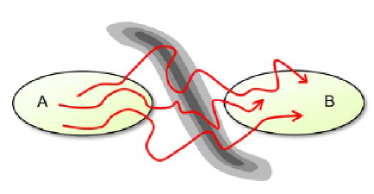
Figure 2: Reactive and product regions of phase-space A and B respectively. System remains in these regions much longer compare to rest of the phase-space, taken from Dellago and Bolhuis .

II Transition Path Reconstructions

The basic machinery of Transition Path Ensemble is formulated by Dellago et. al. Dellago et al. (1999), the formulations can be varied in the literature Weinan and Vanden-Eijnden (2010) but the basic idea is similar.

The basic notion in describing transition paths is shown in Figure 2 where a complex system undergoes a transition from region A to region B in the phase-space. These regions are stable in a sense that system stays considerably long.

Consider a state at time $t$ which is explained with an instantenous trajectory of $N$ particle system

$${\bf x}_{i}(t)=({\bf p}_{1}(t_{i}),{\bf q}_{1}(t_{i}),...,{\bf p}_{N}(t_{i}),{\bf q}_{N}(t_{i})).$$

Introducing an order parameter $\lambda(x)$ may help us to identify region B, where product states are located,

$${\bf x}_{i}(t)\in B\;\;\;if\;\;\lambda_{min}\leq\lambda(x)\leq\lambda_{max}$$

The distribution $P(\lambda,t)$ at time $t$ for trajectories starting in the region A at time $t=0$

$$P(\lambda,t) = \int dx_{0}\rho(x_{0})h_{A}(x_{0})\delta$$ (3)

$$\left[\lambda-\lambda(x_{t})\right]\left(\int dx_{0}\rho(x_{0})h_{A}(x_{0})\right)^{-1}$$

where $\rho(x_{0}$ is the equilibrium phase-space distribution, $h_{A}$ and $h_{B}$ are characteristic functions which are either $1$ or $0$ depending upon if trajectory is inside the region A or B or not inside respectively and $delta$ is the usual Dirac delta-function. The time correlation function $C(t)$ then defined as follows

$$C(t)=\int_{\lambda_{min}}^{\lambda_{max}}d\lambda\;P(\lambda,t)$$ (4)

In order to compute $P(\lambda,t)$ we define $N-1$ overlapping regions $B[i]$ over the order-parameter space, where $B[0]=B$, such that

$${\bf x}_{t}\in B[i]\Leftrightarrow\lambda_{min}[i]\leq\lambda(x)\leq\lambda_{max}[i]$$

where index $i$ ranges $0<i<N$ and region $B[i]$ must have an overlapping windows with $B[i-1]$ and $B[i+1]$, so the probability of reactive trajectories for each region can be written

$$P(\lambda,t;i) = \int dx_{0}f_{AB[i]}(x_{0},t)\delta$$ (5)

$$\left[\lambda-\lambda(x_{t})\right]\left(\int dx_{0}\rho(x_{0})h_{A}(x_{0})\right)^{-1},$$

where this equation is directly proportional to Eq. 3, $f_{AB[i]}$ is called transition path ensemble that describes all initial condition $x_{0}$ in region A leading to trajectories ending in $B[i]$ at time $t$ ;

$$f_{AB[i]}=\rho(x_{0})h_{A}(x_{0})h_{B[i]}(x_{t}).$$

One can compute time correlation function $C(t)$ (implies ability to compute reaction rates) by matching histograms of $P(\lambda,t;i)$ in the overlapping regions to obtain $P(\lambda,t)$. Sampling this path ensemble was an intense research over the last decade.

II.1 Sparse Transition Path Ensemble

Recall the construction of transition path ensemble which has explained shortly. Now, CS framework will be introduced in construction of transition path ensemble. The main idea is to construct $P(\lambda,t;i)$ histograms via CS framework. Consider the histograms as a vector ${\bf P}$ with regular samples $\Delta\lambda$ of $n$-bins.

1. The sparse representation of ${\bf P}$ via an orthogonal transformation $\mathscr{T}$, for example Discrete Fourier Transform or a wavelet bases, can be written as

   $${\bf P}(\lambda,t)=\mathscr{T}{\bf P_{s}},$$ (6)

   ${\bf P_{s}}$ being the sparse representation of the probability $P(\lambda,t;i)$.

2. A CS matrix ${\bf\Phi}$ is formed with an introduction of a Gaussian random measurement matrix $\mathscr{G}$, ${\bf\Phi}=\mathscr{G}\mathscr{T}$, while it is known that random matrices are maximally incoherent to any bases.

3. We define a measurement which is randomly under-sampled histogram of probabilities ${\bf\tilde{P}}(\lambda,t;i)$, having randomly placed (random widths) $m$-bins, $m\ll n$ .

4. An optimization problem formulated as follows;

   $$min\;||\mathscr{T}{\bf P_{s}}||_{1}\;\;\;s.t.\;\;\;{\bf\tilde{P}}={\bf\Phi}{\bf s},$$ (7)

   where unknown Probability ${\bf P}$ will be recovered from this procedure as well as correlation function and reaction rates as a consequence. The above procedure is called compressive transition path sampling .

The proposed method can be used with any of the the path sampling algorithms while the compression is taken place in construction of probability histograms.

III Challenges in Implementation

Some challenges on implementing proposed formalism are discussed.

1. $\ell_{1}$ minimizer: There are available minimizers written for general purpose packages like matlab Berg and Friedlander (2007); Candès and Romberg (2007). For test purposes, mensioned packages would be sufficient, however for larger scale molecular systems distributed implementation is needed.

2. Test systems for sparse trajectory construction One of the simplest system, Lennard-Jones liquid can be used Smit (1992) to demonstrate sparse trajectory construction. For an initial test, only a randomly generated sub-set of obtained trajectory can be used i.e. retaining the physics of the trajectory by using equily-spaced time-step. This means an offline analysis of the trajectory using random parts of it to reconstruct the original data. If this test is successful, the data (trajectory) obtained by randomly spaced time-steps can be tested, see challenges section.

3. Test systems for sparse TPS For inital test purposes, a model system studied previously in the context of transition path sample Dellago et al. (1999), which is called Straub-Borkovec-Berne Straub et al. (1988), can be utilized. Trajectories can be generated via a standard coarse-grained codes such as LAMMPS Plimpton et al. (2007) or NAMD Phillips et al. (2005). It is also an option to use smaller scale snips of codes to make thinks much easier Rapaport (2004) to have a compact tools. Further collection of test systems can also be used Metzner et al. (2006).

4. Realistic System If initial test were successful enough a more realistic simulations can be tested, such as Protein folding Bolhuis (2003).

5. Physics of inverse problem The equations presented for inverse reconstruction for sparse trajectory and sparse histograms in transition paths are based on generic signal recovery. One may argue that the physics behind this approach is not strong enough. However the measurement vectors in both cased are indeed generated via physical process i.e. molecular trajectories. For example in one pixel camera example of CS frame work Baraniuk (2007), voltages generated by the lens is taken granted as measurements that are related to image, so there is no reason not to relate measured under-sampled trajectories to sparse trajectories. But further justification of inverse problems proposed in the previous sections must be developed in more rigorous mathematical terms, probably in the language of Hamiltonian Systems. Monte Carlo sampling was also proposed for inverse problems Mosegaard and Tarantola (1995), this work maybe taken as a reference point.

6. System size In the proposed scheme whole trajectory evolution of $N$-body system is dump into a single vector for sparse trajectory construction. This might be problematic for large systems with too many samples over time, for example 10000 particles with 3 ns simulations with 1 fs needs a storage of more then 3 million elements. However this problem can be solved by introducing and iterative scheme for the minimizer that only needs to store adjacent sampling point i.e. time steps.

7. Using large time-steps The real advantage of sparse recovery can be obtain when random large time-steps is used in producing molecular trajectories on the fly. However in that case, the effect of large time-steps in the integrator and for the physics of the problem might be in question. This problem studied in the literature extensively Winger et al. (2009); Fincham (1986); Macgowan and Heyes (1988).

IV Outlook

We proposed a formalism to use CS in TPS, we can generate results from computer models of rare events very fast. TPS is not only applicable to chemical reactions but on any complex system having a reaction mechanism, from one stable state to another, such as a power grid network into a failure state, a financial market from one state to an other, many more examples from complex networks can be given such as social networks. If an analogous concepts of trajectories and order parameters can be found for the mentioned complex systems. Possible extensions of this formalism to stochastic noisy simulations is also possible where CS shown to work better in noisy environments. A role of information content in transition path techniques can also be addressed.

References

- Allen and Tildesley (1989) M. Allen and D. Tildesley, Computer simulation of liquids (Clarendon Press, 1989).
- Frenkel and Smit (2002) D. Frenkel and B. Smit, Understanding molecular simulation: from algorithms to applications (Academic Pr, 2002).
- Rapaport (2004) D. Rapaport, The art of molecular dynamics simulation (Cambridge Univ Pr, 2004).
- (4) N. Doltsinis, NIC Series, ISBN 3-00-017350 1, 375.
- Landau and Binder (2000) D. Landau and K. Binder, Cambridge, MA/New York (2000).
- Newman and Barkema (1999) M. Newman and G. Barkema, Monte Carlo methods in statistical physics (Oxford University Press, USA, 1999).
- Vanden-Eijnden (2009) E. Vanden-Eijnden, Journal of Computational Chemistry 30, 1737 (2009).
- Shannon (1949) C. E. Shannon, Proceedings of the IRE 37, 10 (1949).
- Nyquist (1928) H. Nyquist, Transactions of the American Institute of Electrical Engineers , 617 (1928).
- Candès et al. (2006) E. J. Candès, J. K. Romberg, and T. Tao, Communications on Pure and Applied Mathematics 59, 1207 (2006).
- Donoho (2006) D. L. Donoho, IEEE Transactions on Information Theory 52, 1289 (2006).
- Eldar and Kutyniok (2012) Y. C. Eldar and G. Kutyniok, Compressed sensing: theory and applications (Cambridge University Press, 2012).
- Eyring (1935) H. Eyring, Chemical Reviews 17, 65 (1935).
- Wigner (1938) E. Wigner, Transactions of the Faraday Society 34, 29 (1938).
- Horiuti (1938) J. Horiuti, Bulletin of the Chemical Society of Japan 13, 210 (1938).
- Hänggi et al. (1990) P. Hänggi, P. Talkner, and M. Borkovec, Reviews of Modern Physics 62, 251 (1990).
- Truhlar et al. (1996) D. Truhlar, B. Garrett, and S. Klippenstein, J. phys. Chem 100, 12771 (1996).
- Schenter et al. (2003) G. Schenter, B. Garrett, and D. Truhlar, The Journal of Chemical Physics 119, 5828 (2003).
- Doll (2005) J. D. Doll, in Handbook of Materials Modeling, edited by S. Yip (Springer Netherlands, 2005) pp. 1573–1583.
- Chong et al. (2017) L. T. Chong, A. S. Saglam, and D. M. Zuckerman, Current opinion in structural biology 43, 88 (2017).
- Jung et al. (2017) H. Jung, K.-i. Okazaki, and G. Hummer, The Journal of chemical physics 147, 152716 (2017).
- Chandler (1978) D. Chandler, The Journal of Chemical Physics 68, 2959 (1978).
- Miller (1998) W. Miller, J. Phys. Chem. A 102, 793 (1998).
- Weinan and Vanden-Eijnden (2010) E. Weinan and E. Vanden-Eijnden, Annual Reviews of Physical Chemistry 61 (2010).
- Pratt (1986) L. Pratt, The Journal of Chemical Physics 85, 5045 (1986).
- Dellago et al. (1998) C. Dellago, P. Bolhuis, F. Csajka, and D. Chandler, The Journal of Chemical Physics 108, 1964 (1998).
- Bolhuis et al. (1998) P. Bolhuis, C. Dellago, and D. Chandler, Faraday Discussions 110, 421 (1998).
- Bolhuis et al. (2002) P. Bolhuis, D. Chandler, C. Dellago, and P. Geissler, Annual Reviews of Physical Chemistry 53 (2002).
- Bolhuis (2003) P. Bolhuis, Proceedings of the National Academy of Sciences of the United States of America 100, 12129 (2003).
- Van Erp et al. (2003) T. Van Erp, D. Moroni, and P. Bolhuis, The Journal of Chemical Physics 118, 7762 (2003).
- Moroni (2005) D. Moroni, Efficient Sampling of Rare Event Pathways, Ph.D. thesis, Universiteit van Amsterdam (2005).
- Chopra et al. (2008) M. Chopra, R. Malshe, A. Reddy, and J. de Pablo, The Journal of chemical physics 128, 144104 (2008).
- (33) C. Dellago and P. Bolhuis, .
- Vanden-Eijnden (2006) E. Vanden-Eijnden, Computer Simulations in Condensed Matter Systems: From Materials to Chemical Biology Volume 1 , 453 (2006).
- (35) P. Metzner, C. Schütte, and E. Vanden-Eijnden, Multiscale Model. Simul. 7, 1192.
- Weinan and Vanden-Eijnden (2006) E. Weinan and E. Vanden-Eijnden, Journal of statistical physics 123, 503 (2006).
- Ren and Vanden-Eijnden (2002) W. Ren and E. Vanden-Eijnden, Phys. Rev. B 66, 1 (2002).
- Weinan et al. (2005) E. Weinan, W. Ren, and E. Vanden-Eijnden, J. Phys. Chem. B 109, 6688 (2005).
- Rogal and Bolhuis (2010) J. Rogal and P. G. Bolhuis, The Journal of Chemical Physics 133, 034101 (2010).
- Dellago et al. (1999) C. Dellago, P. Bolhuis, and D. Chandler, The Journal of Chemical Physics 110, 6617 (1999).
- Berg and Friedlander (2007) E. v. Berg and M. P. Friedlander, “SPGL1: A solver for large-scale sparse reconstruction,” (2007).
- Candès and Romberg (2007) E. Candès and J. Romberg, “L1-magic,” http://www.l1-magic.org (2007).
- Smit (1992) B. Smit, The Journal of Chemical Physics 96, 8639 (1992).
- Straub et al. (1988) J. Straub, M. Borkovec, and B. Berne, The Journal of Chemical Physics 89, 4833 (1988).
- Plimpton et al. (2007) S. Plimpton et al., Sandia National Laboratories (2007).
- Phillips et al. (2005) J. Phillips, R. Braun, W. Wang, J. Gumbart, E. Tajkhorshid, E. Villa, C. Chipot, R. Skeel, L. Kale, and K. Schulten, Journal of Computational Chemistry 26, 1781 (2005).
- Metzner et al. (2006) P. Metzner, C. Schütte, and E. Vanden-Eijnden, The Journal of chemical physics 125, 084110 (2006).
- Baraniuk (2007) R. Baraniuk, Lecture notes in IEEE Signal Processing magazine 24, 118 (2007).
- Mosegaard and Tarantola (1995) K. Mosegaard and A. Tarantola, Journal of Geophysical Research 100, 12431 (1995).
- Winger et al. (2009) M. Winger, D. Trzesniak, R. Baron, and W. Gunsteren, Physical Chemistry Chemical Physics 11, 1934 (2009).
- Fincham (1986) D. Fincham, Computer Physics Communications 40, 263 (1986).
- Macgowan and Heyes (1988) D. Macgowan and D. Heyes, Molecular Simulation 1, 277 (1988).