Controlled Fluidization, Mobility and Clogging in Obstacle Arrays Using Periodic Perturbations

Abstract

We show that the clogging susceptibility and flow of particles moving through a random obstacle array can be controlled with a transverse or longitudinal ac drive. The flow rate can vary over several orders of magnitude, and we find both an optimal frequency and an optimal amplitude of driving that maximizes the flow. For dense arrays, at low ac frequencies a heterogeneous creeping clogged phase appears in which rearrangements between different clogged configurations occur. At intermediate frequencies a high mobility fluidized state forms, and at high frequencies the system reenters a heterogeneous frozen clogged state. These results provide a technique for optimizing flow through heterogeneous media that could also serve as the basis for a particle separation method.

Particle transport through heterogeneous media is relevant to flows in porous media 1 ; 2 , transport of colloidal particles on ordered or disordered substrates 3 ; 4 ; 5 ; 6 ; 7 , clogging phenomena 8 ; 9 ; 10 ; 11 ; 12 ; 13 , filtration 14 ; 15 ; 16 , and active matter motion in disordered environments 17 ; 18 ; 19 ; 20 . It also has similarities to systems that exhibit depinning phenomena when driven over random or ordered substrates 21 . Recent work has focused on clogging effects for particle motion through obstacle arrays, where the onset of clogging is characterized by the formation of a heterogeneously dense state 11 ; 12 ; 13 . Such clogging is relevant for the performance of filters or for limiting the amount of flow through disordered media, so understanding how to avoid clog formation or how to optimize the particle mobility in obstacle arrays is highly desirable. Clogging also occurs for particle flow through hoppers or constrictions, where there can be a transition from a flowing to a clogged state as the aperture size decreases or the flow rate increases 22 ; 23 ; 24 ; 25 ; 26 . The clogging susceptibility in such systems can be reduced with periodic perturbations or vibrations 27 ; 28 ; 29 . Applied perturbations generally produce enhanced flows in disordered systems 30 ; 31 ; N1 ; 32 ; 33 ; however, there are examples where the addition of perturbations or noise can decrease the flow or induce jamming, such as the freezing by heating phenomenon 34 ; 35 or the appearance of a reentrant high viscosity state in vibrated granular matter 36 . A natural question is whether clogging and mobility for particle flows through obstacles can be controlled or optimized with applied perturbations in the same way as hopper flow. The situation is more complex for two-dimensional (2D) disordered obstacle arrays than for hopper geometries since shaking can be applied in either the longitudinal or transverse direction, and one type of shaking may be more effective than the other.

In this work we numerically examine particle flow though a disordered obstacle array where the particles experience both a dc drive and ac shaking. In the absence of the ac shaking, there is a well defined clogging transition at a critical obstacle density $\phi_{c}^{dc}$ above which the flux of particles drops to zero. We find that application of a transverse or longitudinal ac drive above $\phi_{c}^{dc}$ unclogs the system and permits flow to occur, while the mobility drops back to zero at a higher second critical obstacle density $\phi_{c}^{ac}$. We identify an optimal ac frequency for mobility and find that at low frequencies, the system forms a nearly immobile heterogeneous creeping clogged state in which particle rearrangements produce transitions between different clogged configurations. At intermediate frequencies, a more uniform flowing fluidized state appears, and at high frequencies a heterogeneous frozen clogged state emerges in which there are no particle rearrangements. The mobility for fixed frequency and changing ac amplitude is also nonmonotonic. For obstacle densities below $\phi_{c}^{dc}$, the ac drive still strongly affects the flow rate, and we find an optimal frequency that maximizes the flow as well as a local minimum in the mobility produced by a resonance effect of the ac motion with the average spacing between obstacles. In most cases, transverse ac drives produce higher mobility than longitudinal ac drives; however, at low obstacle densities the transverse ac drive reduces the flow. We show that these effects are robust for a wide range of particle densities, and we map a dynamic phase digram describing the fluid regime, the creeping clogged phase, and the frozen clogged state.

Simulation and System— We simulate a 2D system of non-overlapping repulsive particles in the form of disks interacting with a random array of obstacles where the particles are subjected to a dc drift force and an ac shaking force. The sample is of size $L\times L$ with $L=100$ and we impose periodic boundary conditions in the $x$ and $y$ directions. Interactions between pairs of disks $i$ and $j$ are given by the repulsive harmonic force ${\bf F}^{ij}_{dd}=k(r_{ij}-2R_{d})\Theta(r_{ij}-2R_{d}){\hat{\bf r}}_{ij}$, where the disk radius $R_{d}=0.5$, $r_{ij}=|{\bf r}_{i}-{\bf r}_{j}|$, ${\hat{\bf r}}_{ij}=({\bf r}_{i}-{\bf r}_{j})/r_{ij}$, and $\Theta$ is the Heaviside step function. The spring stiffness $k=200$ is large enough that disks overlap by less than one percent, placing us in the hard disk limit as confirmed by previous works 11 ; 12 ; 37 . The obstacles are modeled as immobile disks with the same radius and disk-disk interactions as the mobile particles. There are $N_{m}$ mobile particles with an area coverage of $\phi_{m}=N_{m}\pi R^{2}_{d}/L^{2}$, while the area coverage of the $N_{\rm obs}$ obstacles is $\phi_{\rm obs}=N_{\rm obs}\pi R^{2}_{d}/L^{2}$ and the total area coverage is $\phi_{\rm tot}=\phi_{m}+\phi_{\rm obs}$. For monodisperse disks the system forms a triangular solid at $\phi_{\rm tot}=0.9$ 37 . The obstacles are placed in a dense lattice and randomly diluted until the desired $\phi_{obs}$ is reached, so that the minimum spacing between obstacle centers is $d_{\rm min}=2.0$. The particle dynamics are governed by the following overdamped equation of motion: $\eta d{\bf r}_{i}/dt={\bf F}_{\rm inter}^{i}+{\bf F}_{\rm obs}^{i}+{\bf F}_{dc}+{\bf F}_{ac}$. Here ${\bf F}_{\rm inter}^{i}=\sum_{j=0}^{N_{m}}{\bf F}_{dd}^{ij}$ are the particle-particle interactions, ${\bf F}_{\rm obs}^{i}=\sum_{k=0}^{N_{\rm obs}}{\bf F}_{dd}^{ik}$ are the particle-obstacle interactions, and ${\bf F}_{dc}=F_{dc}{\hat{\bf x}}$ is the dc drift force applied in the positive $x$-direction, where $F_{dc}=0.05$. Each simulation time step is of size $dt=0.002$. We apply a sinusoidal ac drive that is either transverse (perpendicular) to the dc drive, ${\bf F}_{ac}=F_{ac}^{\perp}{\hat{\bf y}}$, or longitudinal (parallel) to the dc drive, ${\bf F}_{ac}=F_{ac}^{||}{\hat{\bf x}}$ . We measure the time average of the velocity per particle in the dc drift direction, $\langle V_{x}\rangle=N_{m}^{-1}\sum^{N_{m}}_{i=1}{\bf v}_{i}\cdot{\hat{\bf x}}$, where ${\bf v}_{i}$ is the velocity of particle $i$. We define the mobility as $M=\langle V_{x}\rangle/\langle V^{0}_{x}\rangle$, where $\langle V^{0}_{x}\rangle$ is the obstacle-free drift velocity, so that in the free flow limit, $M=1.0$. We wait at least $10^{7}$ simulation time steps before taking measurements to ensure that the system has reached a steady state.

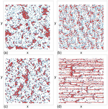
Figure 1: Locations of particles (red) and obstacles (blue) for a system with $\phi_{\rm tot}=0.275$ and an $x$-direction drift force of $F_{dc}=0.05$ under an applied transverse ($y$-direction) ac drive of magnitude $F^{\perp}_{ac}=0.5$ for different ac frequencies $\omega$. (a) A low mobility creeping clogged state with $M=0.01$ at $\omega=10^{-7}$ and $\phi_{\rm obs}=0.1256$. (b) A high mobility fluidized state with $M=0.27$ at $\omega=10^{-4}$ and $\phi_{\rm obs}=0.1256$. (c) A frozen clogged state with $M=0$ at $\omega=10^{-1}$ and $\phi_{\rm obs}=0.1256$. (d) A flowing state at $\omega=10^{-1}$ and $\phi_{\rm obs}=0.047$. The images in (a,b,c) were obtained at the points marked a, b, and c in Fig. 2(b).

Results – In Fig. 1(a) we illustrate the positions of the particles and obstacles in a sample with $F_{dc}=0.05$, $\phi_{\rm tot}=0.275$, and $\phi_{\rm obs}=0.1256$ under a transverse drive of magnitude $F^{\perp}_{ac}=0.5$ in what we define as the low frequency limit of $\omega=10^{-7}$, where the mobility is very small, $M=0.01$. The particles assemble into high density clogged regions separated by large void areas. There are slow rearrangements of the particles but little net motion in the direction of the dc drift, so the system is effectively transitioning between different clogged configurations. At $\omega=10^{-4}$ in Fig. 1(b), the mobility of the same sample reaches its maximum value of $M=0.27$. Here the clustering is reduced compared to what occurs at lower frequencies, and the system is in a partially fluidized state. For the high frequency of $\omega=10^{-1}$ in Fig. 1(c), a completely frozen clogged state with $M=0$ appears. In Fig. 1(d), when $\omega=10^{-1}$ but the obstacle density is reduced to $\phi_{\rm obs}=0.047$, the system is in a flowing state.

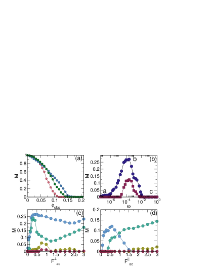
Figure 2: (a) Mobility $M$ vs obstacle density $\phi_{\rm obs}$ for $\phi_{\rm tot}=0.275$ at $F^{\perp}_{ac}=F^{||}_{ac}=0$ (pink), where $M=0$ for $\phi_{\rm obs}>0.115$; at $F^{\perp}_{ac}=0.5$ and $\omega=10^{-4}$ (blue), where $M\approx 0$ for $\phi_{\rm obs}>0.195$; and at $F^{||}_{ac}=0.5$ and $\omega=10^{-4}$ (green), where $M\approx 0$ for $\phi_{\rm obs}>0.155$. (b) $M$ vs ac frequency $\omega$ for the system in Fig. 1(a–c) at $\phi_{\rm tot}=0.275$, $\phi_{\rm obs}=0.1256$, and $F_{ac}=0.5$ for transverse (blue circles) and longitudinal (red squares) ac driving showing a low frequency clogged state, an intermediate frequency flowing state, and a high frequency clogged state. The letters a, b, c mark the frequencies at which the images in Fig. 1(a–c) were obtained. (c) $M$ vs $F^{\perp}_{ac}$ for the system in (b) under transverse driving with $\omega=10^{-4}$ (blue), $10^{-3}$ (green), $10^{-2}$ (gold), and $10^{-1}$ (red). (d) M vs $F_{ac}^{||}$ at the same frequencies as in (c) under longitudinal driving.

In Fig. 2(a) we plot $M$ versus obstacle density $\phi_{\rm obs}$ for a system with $\phi_{\rm tot}=0.275$ for zero ac drive, a transverse ac drive of $F^{\perp}_{ac}=0.5$ at $\omega=10^{-4}$, and a transverse dc drive with $F^{||}_{ac}=0.5$ and $\omega=10^{-4}$. A clogged state with $M=0$ appears for $\phi_{\rm tot}>0.115$ under no ac drive, for $\phi_{\rm tot}>0.2$ under transverse ac driving, and for $\phi_{\rm tot}>0.155$ under longitudinal driving, so there is a wide range of frequencies over which the transverse ac drive is the most effective at reducing clogging. For $\phi_{\rm obs}<0.07$, the transverse ac drive produces a lower mobility $M$ than either the longitudinal or zero ac driving.

In Fig. 2(b) we plot $M$ versus ac frequency $\omega$ for the system from Fig. 1(a–c) with $\phi_{\rm tot}=0.275$ and $\phi_{\rm obs}=0.1256$ for transverse and longitudinal ac driving of magnitude $F_{ac}=0.5$. We find a low mobility state for $\omega<10^{-6}$ and a zero mobility state for $\omega\geq 10^{-2}$. The optimal mobility occurs at a frequency of $\omega\approx 2.5\times 10^{-4}$. Both directions of ac driving produce the same dynamic states, but the maximum value of $M$ for longitudinal driving is less than half that found for transverse driving, and the window of unclogged states is narrower for longitudinal driving. Additionally, the low frequency states with $\omega<10^{-5}$ are fully clogged with $M=0$ for longitudinal driving, but have a small finite mobility for transverse driving. These results indicate that there are two different types of clogged states separated by an intermediate fluidized state in which the mobility reaches its optimum value.

In Fig. 2(c) we plot $M$ versus $F^{\perp}_{ac}$ for a system with $\phi_{\rm tot}=0.275$ and $\phi_{\rm obs}=0.1256$ at the optimal frequency of $\omega=10^{-4}$ and at $\omega=10^{-3}$, $10^{-2}$, and $10^{-1}$. For each driving frequency, there is an optimal value of $F^{\perp}_{ac}$ that maximizes $M$. Figure 2(d) shows $M$ versus $F^{||}_{ac}$ for the same system at the same driving frequencies. At $\omega=10^{-4}$, $M$ initially increases with $F^{||}_{ac}$ but it then decreases until the system reaches a clogged state with $M=0$ for $F^{||}_{ac}>1.5$. Previous studies of particles moving over randomly placed obstacles under a purely dc drive have shown that negative differential conductivity or a zero mobility state can appear at high dc drives 38 ; 39 ; 40 ; 41 . In our system we find a similar effect under large longitudinal ac drives, so that in general the system reaches a clogged state for high $F^{||}_{ac}$. For $\omega=10^{-3}$ in Fig. 2(d), $M$ increases monotonically over the range of $F^{||}_{ac}$ shown; however, $M$ does decrease for much larger values of $F^{||}_{ac}$. In general, $M$ is higher for transverse ac driving since the transverse shaking permits the particles to more easily move around obstacles, whereas for longitudinal ac driving, the particles are pushed toward the obstacles and $M$ is reduced.

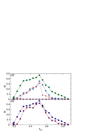
Figure 3: (a) $M$ vs $\phi_{\rm tot}$ for $\phi_{\rm obs}=0.1256$ and $F^{\perp}_{ac}=0.5$ at $\omega=5.0\times 10^{-6}$ (black squares), $10^{-4}$ (red circles), $10^{-2}$ (green diamonds) and $10^{-1}$ (blue triangles). Over the entire range of $\phi_{\rm tot}$, the $\omega=10^{-4}$ curve has the highest values of $M$. (b) $M$ vs $\phi_{\rm tot}$ in the same system for transverse (blue circles) and longitudinal (red squares) ac driving at $\omega=10^{-4}$, where transverse ac driving produces the highest values of $M$.

In Fig. 3(a) we plot $M$ versus $\phi_{\rm tot}$ for samples with $\phi_{\rm obs}=0.1256$ and $F^{\perp}_{ac}=0.5$ at $\omega=5.0\times 10^{-6}$, $10^{-4}$, $10^{-2}$, and $10^{-1}$. $M$ is always small at low $\phi_{\rm tot}$, increases to a local maximum at $\phi_{\rm tot}=0.5$, and decreases to zero as $\phi_{\rm tot}$ approaches $\phi_{\rm tot}=0.85$, corresponding to the density at which the system starts to form a crystallized solid state 37 ; 42 . We find the highest mobility for $\omega=10^{-4}$, particularly for $0.66<\phi_{\rm tot}<0.85$ where $M$ is close to zero for $\omega=10^{-2}$ and $10^{-1}$. In Fig. 3(b) we show $M$ versus $\phi_{\rm tot}$ at $\omega=10^{-4}$ for transverse and longitudinal ac driving, where we again find that the transverse ac driving gives higher values of $M$ for all $\phi_{\rm tot}$ and where the local maximum in $M$ falls at $\phi_{\rm tot}=0.5$ for both ac driving directions.

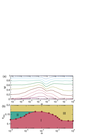
Figure 4: (a) $M$ vs $\omega$ for samples with $\phi_{\rm tot}=0.275$ and $F^{\perp}_{ac}=0.5$ at $\phi_{\rm obs}=0.00157$, 0.031416, 0.047124, 0.062831, 0.07754, 0.09424, 0.1099, 0.12566, 0.14137, and $0.157$, from top to bottom. (b) Dynamic phase diagram as a function of $\phi_{\rm obs}$ vs $\omega$ for transverse driving with $F^{\perp}_{ac}=0.5$. I: flowing fluidized state; II: creeping clogged state; III: frozen clogged state.

In Fig. 4(a) we plot $M$ versus $\omega$ in samples with $\phi_{\rm tot}=0.275$ and $F^{\perp}_{ac}=0.5$ at $\phi_{\rm obs}=0.00157$ to $0.157$. For $\phi_{\rm obs}>0.1099$, the system reaches a fully clogged state with $M=0$. We define the onset of the low frequency clogged state as the point at which $M<0.02$. A local maximum in $M$ appears near $\omega=2.5\times 10^{-4}$ and shifts to slightly lower frequencies as $\phi_{\rm obs}$ decreases. A local minimum near $\omega=10^{-3}$ develops when $\phi_{\rm obs}<0.1099$, and this minimum also shifts to lower frequencies with decreasing $\phi_{\rm obs}$. Both of the local extrema are correlated with characteristic length scales of the system. The local maximum at $\phi_{\rm obs}=0.1256$ falls at a value of $\omega$ for which the distance $d_{\tau}=\omega^{-1}dt(F_{ac}^{\perp}/\sqrt{2}+F_{dc})$ a particle moves during a single ac cycle matches the average spacing $1/\sqrt{\phi_{\rm obs}}$ between obstacles. As this average spacing decreases for increasing $\phi_{\rm obs}$, the frequency at which the maximum value of $M$ occurs decreases as well. The frequency at which the local minimum appears for $\phi_{\rm obs}<0.1099$ corresponds to the point at which $d_{\tau}$ matches the minimum transverse surface-to-surface obstacle spacing of $d_{\rm min}-2R_{d}$. At this matching frequency, the particles preferentially collide with the obstacles rather than moving between them or around them, reducing the mobility. The two resonant frequencies are separated by a factor of 10 since $F^{\perp}_{ac}/F_{dc}=10$.

In Fig. 4(b) we plot a dynamic phase diagram as a function of $\phi_{\rm obs}$ versus $\omega$ for samples with $F^{\perp}_{ac}=0.5$. Here phase I is the flowing fluidized state, phase II is the low frequency creeping clogged state, and phase III is the frozen clogged state. For $\phi_{\rm obs}>0.165$, the spacing between obstacles becomes so small that the system is in a frozen state for all values of $\omega$. The fluidized state is of maximum extent between $\omega=10^{-5}$ and $\omega=10^{-4}$. The dynamic phase diagram for longitudinal ac driving (not shown) is similar; however, the extent of phase I is reduced.

Our results resemble what has been found in recent experiments on the viscosity of vibrated granular matter, where the system is in a jammed state for low vibration frequencies, enters a low viscosity fluid state at intermediate frequencies, and shows a reentrant jammed state at high frequencies 36 . Other studies have also revealed optimal frequencies for dynamic resonances in granular matter, where the speed of sound is the lowest at intermediate frequencies when the grains are the least jammed 43 .

Our results show that the clogging and flow of particulate matter moving through heterogeneous media can be controlled with ac driving, which could be applied to colloidal particles moving through disordered or porous media. Since the mobility is a function of the driving frequency, ac driving could be used to separate different particle species when one species is in a low mobility or clogged state for a given frequency while the other is in a high mobility state. These results can be generalized to the depinning dynamics in many other systems such as active matter, vortices in superconductors, or frictional systems, where there is a competition between the collective interactions of the particles and quenched disorder in the substrate.

Summary— We have examined the clogging and flow of particles moving through random obstacle arrays under a dc drift and an additional transverse or longitudinal ac drive. At zero ac driving, there is a well defined obstacle density above which the system reaches a clogged state. When ac driving is added, this clogging transition shifts to much higher obstacle densities. For large obstacle densities, we find a low frequency creeping clogged state where the particles undergo rearrangements from one clogged configuration to another with a drift mobility that is nearly zero. At intermediate frequencies, the particles form a high mobility fluidized state, while at high frequencies, a zero mobility frozen clogged state appears, so that there is an optimal mobility at intermediate frequencies. The mobility is also nonmonotonic as a function of ac driving amplitude for fixed ac driving frequency. In most cases the transverse ac driving is more effective at increasing the mobility than longitudinal ac driving. When the ac amplitude and frequency are both fixed, we find that there is an optimal disk density that maximizes the mobility, while for high disk densities the system enters a low mobility jammed state. At low obstacle densities the system is always in a flowing state; however, for transverse ac driving we find a resonant frequency with reduced flow when the magnitude of the transverse oscillations matches the minimum transverse spacing of the obstacles. We map a dynamic phase diagram showing the locations of the flowing state, creeping clogged state, and frozen clogged state. Our results suggest that ac driving could be used to avoid clogging and to optimize particle flows in disordered media, and this technique could also be used as a method for separating different species of particles. Our results can be generalized for controlling flows in a wide class of collectively interacting particle systems in heterogeneous environments, including colloids, bubbles, granular matter, vortices in superconductors, and skyrmions in chiral magnets.

- (1) L.M. McDowell-Boyer, J.R. Hunt, and N. Sitar, Water Resour. Res. 22, 1901 (1986).
- (2) D.C. Mays and J.R. Hunt, Environ. Sci. Technol. 39, 577 (2005).
- (3) L.R. Huang, E.C. Cox, R.H. Austin, and J.C. Sturm, Science 304, 987 (2004).
- (4) P. Tierno, T.H. Johansen, and T.M. Fischer, Phys. Rev. Lett. 99, 038303 (2007).
- (5) Z. Li and G. Drazer, Phys. Rev. Lett. 98, 050602 (2007).
- (6) R. Zhang and J. Koplik, Phys. Rev. E 85, 026314 (2012).
- (7) J. McGrath, M. Jimenez, and H. Bridle, Lab Chip 14, 4139 (2014).
- (8) H.M. Wyss, D.L. Blair, J.F. Morris, H.A. Stone, and D.A. Weitz, Phys. Rev. E 74, 061402 (2006).
- (9) F. Chevoir, F. Gaulard, and N. Roussel, Europhys. Lett. 79, 14001 (2007).
- (10) G.C. Agbangla, P. Bacchin, and E. Clement, Soft Matter 10, 6303 (2014).
- (11) H. T. Nguyen, C. Reichhardt, and C.J.O. Reichhardt, Phys. Rev. E 95, 030902(R) (2017).
- (12) H. Peter, A. Libal, C. Reichhardt, and C.J.O. Reichhardt, arXiv:1712.03307.
- (13) R.L. Stoop and P. Tierno, arXiv:1712.05321.
- (14) S. Redner and S. Datta, Phys. Rev. Lett. 84, 6018 (2000).
- (15) N. Roussel, T. L. H. Nguyen, and P. Coussot, Phys. Rev. Lett. 98, 114502 (2007).
- (16) C. Barré and J. Talbot, J. Stat. Mech. 2017, 043406 (2017).
- (17) O. Chepizhko, E.G. Altmann, and F. Peruani, Phys. Rev. Lett. 110, 238101 (2013).
- (18) C. Bechinger, R. Di Leonardo, H. Löwen, C. Reichhardt, G. Volpe, and G. Volpe, Rev. Mod. Phys. 88, 045006 (2016).
- (19) A. Morin, N. Desreumaux, J.-B. Caussin, and D. Bartolo, Nat. Phys.13 , 63 (2017).
- (20) Cs. Sándor, A. Libál, C. Reichhardt, and C.J.O. Reichhardt, Phys. Rev. E 95, 032606 (2017).
- (21) C. Reichhardt and C.J.O. Reichhardt, Rep. Prog. Phys 80, 026501 (2017).
- (22) K. To, P.-Y. Lai, and H. K. Pak, Phys. Rev. Lett. 86, 71 (2001).
- (23) I. Zuriguel, L. A. Pugnaloni, A. Garcimartín, and D. Maza, Phys. Rev. E 68, 030301(R) (2003).
- (24) D. Chen, K. W. Desmond, and E. R. Weeks, Soft Matter 8, 10486 (2012).
- (25) I. Zuriguel et al., Sci. Rep. 4, 7324 (2014).
- (26) R. C. Hidalgo, A. Goñi-Arana, A. Hernández-Puerta, and I. Pagonabarraga, Phys. Rev. E 97, 012611 (2018).
- (27) C. Mankoc, A. Garcimartín, I. Zuriguel, D. Maza, and L. A. Pugnaloni, Phys. Rev. E 80, 011309 (2009).
- (28) C. Lozano, G. Lumay, I. Zuriguel, R. C. Hidalgo, and A. Garcimartín, Phys. Rev. Lett. 109, 068001 (2012).
- (29) A. Janda, D. Maza, A. Garcimartín, E. Kolb, J. Lanuza, and E. Clément, Europhys. Lett. 87, 24002 (2009).
- (30) J.A. Dijksman, G.H. Wortel, L.T.H. van Dellen, O. Dauchot, and M. van Hecke, Phys. Rev. Lett. 107, 108303 (2011).
- (31) M. Griffa, E. G. Daub, R. A. Guyer, P. A. Johnson, C. Marone, and J. Carmeliet, Europhys. Lett. 96, 14001 (2011).
- (32) H. Lastakowski, J.-C. Géminard, and V. Vidal, Sci. Rep. 5, 13455 (2015).
- (33) K. To and H.-T. Tai, Phys. Rev. E 96, 032906 (2017).
- (34) G. A. Patterson, P. I. Fierens, F. Sangiullano Jimka, P. G. König, A. Garcimartín, I. Zuriguel, L. A. Pugnaloni, and D. R. Parisi, Phys. Rev. Lett. 119, 248301 (2017).
- (35) D. Helbing, I.J. Farkas, and T. Vicsek, Phys. Rev. Lett. 84, 1240 (2000).
- (36) J.M. Pastor, A. Garcimartín, P.A. Gago, J.P. Peralta, C. Martín-Gómez, L.M. Ferrer, D. Maza, D.R. Parisi, L.A. Pugnaloni, and I. Zuriguel, Phys. Rev. E 92, 062817 (2015).
- (37) A. Gnoli, L. de Arcangelis, F. Giacco, E. Lippiello, M.P. Ciamarra, A. Puglisi, and A. Sarracino, Phys. Rev. Lett. 120, 138001 (2018).
- (38) C. Reichhardt and C.J.O. Reichhardt, Soft Matter 10, 2932 (2014).
- (39) S. Leitmann and T. Franosch, Phys. Rev. Lett. 111, 190603 (2013).
- (40) U. Basu and C. Maes, J. Phys. A: Math. Theor. 47, 255003 (2014).
- (41) O. Bénichou, P. Illien, G. Oshanin, A. Sarracino, and R. Voituriez, Phys. Rev. Lett. 113, 268002 (2014).
- (42) M. Baiesi, A.L. Stella, and C. Vanderzande, Phys. Rev. E 92, 042121 (2015).
- (43) A. J. Liu and S. R. Nagel, Annu. Rev. Condens. Matter Phys. 1, 347 (2010).
- (44) C.J.O. Reichhardt, L.M. Lopatina, X. Jia, and P.A. Johnson, Phys. Rev. E 92, 022203 (2015).