Sector models—A toolkit for teaching general relativity: III. Spacetime geodesics

Abstract

Sector models permit a model-based approach to the general theory of relativity. The approach has its focus on the geometric concepts and uses no more than elementary mathematics. This contribution shows how to construct the paths of light and free particles on a spacetime sector model. Radial paths close to a black hole are used by way of example. We outline two workshops on gravitational redshift and on vertical free fall, respectively, that we teach for undergraduate students. The workshop on redshift does not require knowledge of special relativity; the workshop on particles in free fall presumes familiarity with the Lorentz transformation. The contribution also describes a simplified calculation of the spacetime sector model that students can carry out on their own if they are familiar with the Minkowski metric. The teaching materials presented in this paper are available online for teaching purposes at www.spacetimetravel.org.

Keywords: general relativity, geodesics, gravitational redshift, black hole, sector models

1 Introduction

In view of the goal of teaching introductory general relativity without going beyond elementary mathematics, we are developing an approach based on a particular class of physical models, so-called sector models. The approach relies on the fact that general relativity is a geometric theory and is therefore accessible to intuitive geometric understanding. In the first part of this series, we have developed sector models as physical models of curved spaces and spacetimes (Zahn and Kraus 2014, in the following referred to as paper I). Sector models implement the description of curved spacetimes used in the Regge calculus (Regge 1961) by way of physical models. Sector models can be two-dimensional (e.g. a symmetry plane of a spherically symmetric star), three-dimensional (e.g. the three-dimensional curved space in the exterior region of a black hole), or 1+1-dimensional (i.e. a spacetime with two spatial dimensions suppressed, similar to the Minkowski diagrams of special relativity). Figure 1 illustrates the basic principle using a sphere by way of example: The curved surface is subdivided into small elements of area, in this case quadrilaterals (figure 1(a)). The edge lengths are determined for each quadrilateral. Quadrilaterals in the plane are constructed with the same edge lengths (figure 1(b)). These are the sectors that make up the sector model. The sector model is an approximation to the curved surface, its accuracy being determined by the resolution of the subdivision. For pedagogical purposes, a relatively coarse resolution is useful. Using sector models, the geometry of the respective space or spacetime can be studied with graphical methods. This includes the construction of geodesics as described in the second paper of this series (Zahn and Kraus 2018, in the following referred to as paper II). The construction implements the determination of geodesics according to the Regge calculus (Williams and Ellis 1981). The basic principle is illustrated in figure 1(c). Based on the definition of a geodesic as a locally straight line, the geodesic is drawn using pencil and ruler: Inside a sector, a sector being a flat element of area, a geodesic is a straight line. When the line reaches the border of the sector, the neighbouring sector is joined and the line is continued straight across the border. Sector models are computed true to scale, therefore, the properties read off from them are quantitatively correct, within the discretization error. The accuracy achievable for geodesics is studied in paper II.

General relativity describes the paths of light and free particles as geodesics in spacetime. This contribution shows how geodesics in spacetime can be constructed using spacetime sector models as tools. Radial geodesics close to a black hole are used by way of example. We outline two workshops the way that we teach them for undergraduate students. In the workshop on gravitational redshift (section 2), null geodesics are constructed and the phenomenon of gravitational redshift is inferred. The workshop on radial free fall (section 3) includes the construction of radial timelike geodesics and a comparison with the Newtonian descriptions of free fall and of tidal forces. Conclusions and outlook follow in section 4.

Figure 1: A sector model and the construction of a geodesic using a sphere by way of example. The curved surface is subdivided into small elements of area (a). Their edge lengths are determined and the sectors are constructed as flat pieces with the same edge lengths (b). A geodesic is constructed as a locally straight line using pencil and ruler (c).

2 Workshop on gravitational redshift

In this workshop, world lines of light are constructed as geodesics in spacetime. The construction shows how gravitational redshift arises. A black hole is used by way of example, because in its vicinity the effects are large and are clearly visible in the graphical representation. The construction of geodesics is restricted to radial paths; in the representation of the spacetime the other two spatial directions are suppressed so that the spacetime sector model is 1+1-dimensional.

The workshop presumes that the participants are familiar with the concept of a geodesic as a locally straight line and with sector models as representations of surfaces with curvature. A knowledge of special relativity is not required for this workshop. Minkowski diagrams do play a role and if necessary they are explained to the extent that they are needed in the workshop: Firstly they are introduced as path-time diagrams that differ from the familiar diagrams used in Newtonian mechanics by the fact that the vertical axis is the time axis. In order to familiarize the participants with this representation, we show a diagram with world lines that tell a little story and ask the participants to recount what happens (an example of such a diagram is available online, Kraus and Zahn 2018). Secondly, the units of the axes are addressed, being chosen to make motion at the speed of light run at $45^{\circ}$ in the diagram. Finally the terms event, world line and light cone are introduced.

2.1 Redshift close to a black hole

Figure 2: Sector model for the spacetime of a radial ray in the exterior region of a black hole. (a) Radial ray. (b) Spacetime sector model for the segment marked in (a). The edge on the left represents events at point A, the edge on the right events at point B. The diagonal lines mark the light cone. The model can be extended in time by adding identical sectors.

The workshop begins with the explanation that general relativity describes the paths of light and free particles as geodesics in spacetime. Then a sector model is introduced that represents the spacetime of a radial ray in the exterior region of a black hole. The participants can calculate the sector model themselves (section 2.2) or can be provided with a worksheet (available online, Kraus and Zahn 2018). In a thought experiment the sector model is created from measurements taken close to a black hole: Astronauts travel to a black hole and take up positions along a radial ray. They choose a number of events at these positions and use them as vertices for subdividing the spacetime of the radial ray into quadrilaterals. In order to define an individual quadrilateral, two positions are chosen on the radial ray (figure 2(a)). Two events at the inner position and two at the outer position make up the four vertices. Each quadrilateral is represented by a sector of a Minkowski space (figure 2(b)); the ensemble of sectors makes up the sector model. Since the black hole spacetime is static (we consider a non-rotating black hole), it is possible to choose a subdivision of the spacetime for which the shape of the sectors is independent of time (see section 2.2). This is here implemented, so that the sector model can be arbitrarily extended in time by adding identical sectors.

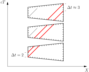
Figure 3: World lines of two light signals propagating radially outwards. An observer at the inner rim of the sectors (left) sends the signals at an interval of two time units. An observer at the outer rim (right) receives them about three time units apart.

The first construction on the sector model is the world line of a light signal propagating radially outwards. Starting from the bottom left corner of the model, a locally straight line is drawn in the direction of the light cone (figure 3, bottom line). Within the sector, the line is straight. When the line reaches the border of the sector, the position of the border point is copied onto the respective border of the neighbouring sector and the line is continued from there. The borders are provided with equidistant tick marks to facilitate the transfer of the border points. The direction in the neighbouring sector is again prescribed by the light cone, since we are concerned with a world line of light.

In the second step the transmission of two consecutive light signals is studied. An observer positioned close to the black hole and at a constant distance (point A at the inner rim of the sectors, see figure 2), sends two light signals outwards, one a short time after the other. In figure 3 the time interval is two time units. A second observer positioned farther away from the black hole and also at a constant distance (point B at the outer rim of the sectors), receives the two signals. In order to find the time interval of the light signals upon reception, the world line of the other signal is added to the diagram (figure 3, top line). The interval of the signals can then be read off and amounts to a little over three time units. If one interprets the two signals as consecutive wave crests of an electromagnetic wave, one concludes from the diagram that the wave is received with an increased period by the outer observer. Thus, radiation receding from a black hole is redshifted. The ratio of the periods $P_{\rm outer}$ and $P_{\rm inner}$ at points B and A, respectively, read off from the construction on the sector model, is $P_{\rm outer}/P_{\rm inner}\approx 1.5$. The calculated exact value is $P_{\rm outer}/P_{\rm inner}=\sqrt{(1-r_{\mathrm{S}}/r_{\rm outer})/(1-r_{\mathrm{S}}/r_{\rm inner})}=1.73$, where $r_{\rm inner}=1.25\,r_{\mathrm{S}}$ and $r_{\rm outer}=2.5\,r_{\mathrm{S}}$ are the radial coordinates of points A and B, respectively. The graphically determined value is too small by 13%; this deviation is due to the relatively coarse resolution of the sector model.

2.2 Calculation of the spacetime sector model

A simplified calculation of sector models is introduced in paper II (section 2.4) for curved surfaces and is here extended to the 1+1-dimensional case. This calculation presumes knowledge of the Minkowski metric. Using the simplified method students can calculate sector models on their own using elementary mathematics only. This enables them to use sector models as tools for studying other curved spacetimes when given their metric. The approximations of the simplified method are discussed in paper II.

The starting point of the construction is the metric

$$\mathrm{d}s^{2}=-\left(1-\frac{r_{\mathrm{S}}}{r}\right)c^{2}\mathrm{d}t^{2}+\frac{1}{1-r_{\mathrm{S}}/r}\mathrm{d}r^{2}$$ (1)

with the usual Schwarzschild coordinates $t$ and $r$ and the Schwarzschild radius $r_{\mathrm{S}}=2GM/c^{2}$ of the central mass $M$, where $G$ is the gravitational constant and $c$ the speed of light.

Figure 4: Calculation of the spacetime sector model of a radial ray. (a) The subdivision of the spacetime in coordinate space. (b) Each sector is constructed in the shape of a symmetric trapezium.

In space the sector model represents a segment of a radial ray from $r=1.25\,r_{\mathrm{S}}$ to $r=2.5\,r_{\mathrm{S}}$ with coordinate length $\Delta r=1.25\,r_{\mathrm{S}}$. The time coordinate $t$ is subdivided into segments of length $\Delta t$ with $c\Delta t=1.25\,r_{\mathrm{S}}$ (figure 4(a)). Since the metric is independent of the time coordinate, only a single segment in time needs to be calculated.

The calculation of the edge intervals yields

$$\Delta s_{t}^{2}(r)=-\left(1-\frac{r_{\mathrm{S}}}{r}\right)c^{2}\Delta t^{2}\hskip 28.45274pt(\Delta r=0)$$ (2)

for the timelike edges and

$$\Delta s_{r}^{2}=\frac{1}{(1-r_{\mathrm{S}}/r_{\mathrm{m}})}\,\Delta r^{2}\hskip 28.45274pt(\Delta t=0)$$ (3)

for the spacelike edges, where the metric coefficient is evaluated at the mean coordinate $r_{\mathrm{m}}=(r_{1}+r_{2})/2$ with the coordinates $r_{1}$ and $r_{2}$ of the associated vertices. Since the sector model is a column of identical sectors, each sector is constructed with the corresponding time symmetry: As shown in figure 4(b), the bases of a trapezium are drawn in direction of the time axis with the lengths $b_{1}=\sqrt{-\Delta s_{t}^{2}(r=1.25\,r_{\mathrm{S}})}$ and $b_{2}=\sqrt{-\Delta s_{t}^{2}(r=2.5\,r_{\mathrm{S}})}$. The height $h$ of the trapezium is determined from the condition that the lateral sides have the interval $\Delta s_{r}^{2}$ (figure 4(b)):

$$\Delta s_{r}^{2}=-\left(\frac{b_{2}-b_{1}}{2}\right)^{2}+h^{2}.$$ (4)

The result is the sector shown in figure 2.

3 Workshop on particle paths

In this workshop world lines are constructed for freely falling particles close to a black hole. As in the previous section the study is restricted to radial paths, so that it is possible to use a 1+1-dimensional spacetime sector model. By means of the particle paths, the connection between the relativistic and the classical descriptions of motion in a gravitational field is pointed out. The workshop presumes that the participants are familiar with the Lorentz transformation.

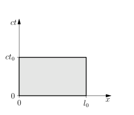
Figure 5: Graphic representation of a spacetime sector in two different reference frames. The events are located inside a spaceship of length $l_{0}$ at spaceship proper times between zero and $t_{0}$. (a) Representation in the rest frame of the spaceship. (b) Representation in the rest frame of a space station that the spaceship passes with velocity $v=0.3\,c$ ($\gamma=1/\sqrt{1-v^{2}/c^{2}}$).

3.1 The construction of timelike geodesics

To study the paths of freely falling particles in the vicinity of a black hole, their world lines are constructed on a sector model. As in the previous examples, the geodesics are drawn as straight lines within each sector and after reaching the boundary are continued in the neighbouring sector. Other than for the null geodesics discussed in section 2, the direction in the neighbouring sector is not predetermined by the light cone. Therefore, it is necessary to join the neighbouring sector and to continue the line straight across the boundary. The joining of two sectors is more complex in spacetime than in the purely spatial case. Clearly, rotating the neighbouring sector into a suitable position is not an option: Since the speed of light has the same value in both sectors, their light cones must coincide. This fixes the orientation of the neighbouring sector.

In the workshop we use a specific example for a spacetime sector in order to introduce the way that neighbouring sectors can be joined. We consider a long and very thin spaceship of rest length $l_{0}$. We define a spacetime sector that is made up of all events that are inside the spaceship and at spaceship proper times between zero and $t_{0}$. The participants draw this spacetime sector in a Minkowski diagram, first in the rest frame of the spaceship (figure 5(a)), then in the rest frame of a space station that the spaceship passes at constant relative velocity (figure 5(b)). The geometric shape of the sector, i.e., the geometric shape drawn on paper and understood in the euclidean sense, clearly depends on the frame of reference. Figures 5(a) and (b) are two different representations of one and the same spacetime sector. One turns into the other under a Lorentz transformation.

Figure 6: Joining two spacetime sectors of the sector model shown in figure 2. The upper sector has been Lorentz-transformed in such a way that it can be joined to the lower sector ($v/c=0.21$).

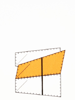
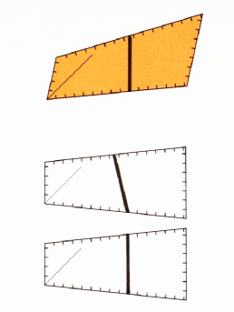
Figure 7: Construction of a geodesic on the spacetime sector model. (a) A sector that has undergone Lorentz transformation serves as transfer sector (in colour). (b) The geodesic is continued straight onto the transfer sector. (c) The line is copied from the transfer sector onto the neighbouring sector in the original symmetric shape.

This permits the joining of sectors: The neighbouring sector is brought into the appropriate form by Lorentz transformation (figure 6). Thus, the transformation that permits the joining of the neighbouring sector is a rotation in the spatial case and a Lorentz transformation in the spacetime case.

When drawing geodesics, it is convenient to use a transformed sector in the role of transfer sector (paper II, section 2.3): When a geodesic reaches the border of a sector (figure 7(a)), it is continued as a straight line across the border onto the transfer sector joined to the respective edge (figure 7(b)) and is then transferred onto the neighbouring sector in its original shape (figure 7(c)). This transfer amounts to reversing the Lorentz transformation. In doing so, straight lines are mapped onto straight lines. Therefore, using the tick marks at the borders, the end points of the line are transferred onto the target sector and are then connected by a straight line (figure 7(c)).

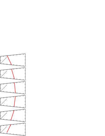
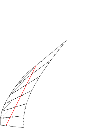
Figure 8: Vertical free fall. (a) A geodesic constructed on the sector model. (b) When all sectors are joined, the world line can clearly be seen to be straight.

3.2 Vertical free fall

Close to a black hole, a particle is thrown upwards. Its path is to be determined. Intuitively, it is clear that the particle reaches a maximum height and then falls back down (provided its initial velocity is less than the escape velocity).

In the relativistic description, the particle, being in free fall, follows a geodesic, i.e., its world line is locally straight. How can these two statements—straight world line on the one hand and up-and-down motion on the other hand—be compatible?

For the construction of the world line, the sector model shown in figure 2 is used with six rows plus an appropriately transformed transfer sector (figure 6). After choosing an initial position and a timelike outward direction, the world line is constructed as a geodesic on the sector model (figure 8(a)): The locally straight line at first leads away from the black hole and then comes closer again. The spacetime geodesic thus provides the expected up-and-down motion in space. In addition, figure 8(b) shows the sector model with all the sectors joined, so that the straightness of the line is obvious. In order to draw the geodesic at a stretch as in this figure, one needs several representations of the sector that are obtained by Lorentz transformations with different velocities. The construction on the sector model displays both the straight line in spacetime and the up-and-down motion in space, and so makes the connection between them quite clear.

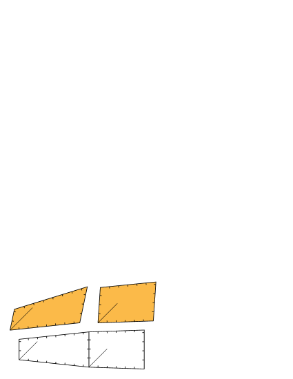
Figure 9: Spacetime sector model for a radial ray in the exterior region of a black hole. (a) Subdivision of the spacetime in coordinate space. (b) Sectors in symmetric form (bottom) and suitably Lorentz-transformed transfer sectors (top). This is an extension of the model shown in figure 2 by a second column with the associated transfer sector (right hand side, $v/c=0.067$). The model can be extended in time by adding identical rows.

3.3 Tidal forces and the curvature of spacetime

When the present workshop on particle paths is combined with the workshop on curvature described in paper I, it is possible to illustrate the physical significance of spacetime curvature with the help of geodesics. For this purpose a second column is added to the sector model shown in figure 2, so that the model now covers the radial ray between $1.25\,r_{\mathrm{S}}$ and $3.75\,r_{\mathrm{S}}$ in two columns (figure 9). The model is used with eight rows plus a transfer sector for each column.

In a local inertial frame momentarily at rest with respect to the black hole, we consider two particles that are slightly displaced in the radial direction. They are released from rest simultaneously, so that they fall one after another radially into the black hole. In the classical description the gravitational force decreases outwards. Therefore, at each instant the outer particle experiences a smaller acceleration than the inner one, so that the two freely falling particles are accelerated relative to each other: As a result of tidal forces, the relative velocity of the particles increases.

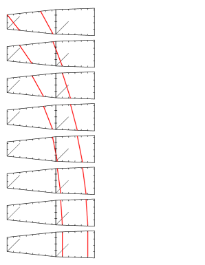
Figure 10: The world lines of two particles that are simultaneously released from rest and fall one after another towards a black hole.

In the general relativistic description, the world lines of the two particles are geodesics that are initially parallel. These geodesics are constructed on the sector model (figure 10). Both world lines start in the direction of the local time axis (figure 10, bottom row). The two initially parallel world lines diverge more and more indicating a relative velocity that increases.

The construction elucidates the origin of the divergence: The world lines are parallel up to the point where they pass a vertex on different sides (figure 10, row 4 to row 5 from the bottom). Each additional vertex between the world lines increases the difference in direction, i.e., increases the relative velocity.

Figure 11 shows the run of a pair of geodesics close to a single vertex in more detail. For clarity, sectors with double coordinate length in time are used ($c\Delta t=2.5\,r_{\mathrm{S}}$). In figures 11(a) and (b) the sectors are joined along the geodesic on the left and on the right, respectively (the upper row being suitably Lorentz-transformed as a whole in each case); in figure 11(c) the sectors are arranged symmetrically.

As described in paper I, in a sector model the so-called deficit angles of the vertices represent curvature. The deficit angle of the vertex considered here is apparent in figures 11(a) and (b) as the gap that remains when the four adjacent sectors are joined around the vertex. This deficit angle is in a spacelike direction and is positive; with the metric signature used here, by convention, this means positive spacetime curvature. By construction, the angle between the two lines behind the vertex depends on the deficit angle. Thus, figures 10 and 11 show that positive spacetime curvature is linked with the divergence of initially parallel world lines; the opposite holds in the case of negative curvature. Spacetime curvature is less intuitive than spatial curvature. However, the run of neighbouring geodesics provides a criterion that can be understood geometrically. Thus the construction shows how the relative acceleration of the two particles comes about in the relativistic description. It can be traced back to the deficit angles at the vertices, i.e. to curvature. This elucidates the physical meaning of spacetime curvature: It corresponds to the Newtonian tidal force.

In addition, figure 11(d) shows the behaviour of initially parallel spacelike geodesics near the same vertex: After the vertex they converge. The opposing behaviour of timelike and spacelike geodesics reflects the corresponding properties of the deficit angles in timelike and spacelike directions, respectively (paper I, section 4).

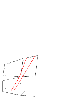
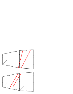
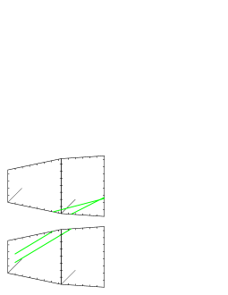
Figure 11: Initially parallel geodesics that pass a vertex on opposite sides subsequently are no longer parallel. In (a) the sectors are joined along the geodesic on the left and in (b) along the geodesic on the right; in (c) they are arranged symmetrically. (d) Spacelike geodesics show the opposite behaviour. (Sector model as in figure 9, but with double coordinate length in time, $c\Delta t=2.5\,r_{\mathrm{S}}$.)

3.4 The construction of geodesics using transfer double sectors

When geodesics are constructed as described above, in some cases the line segment within a sector is very short because it passes close to a vertex (e.g., in figure 10, 4th row from the bottom, left line). In this case the further construction is quite imprecise because the subsequent direction is determined from this short segment. The problem can be solved by using not a single transfer sector but a double one (figure 12). This is built by joining a sector of the neighbouring column, after appropriate Lorentz transformation, to a transfer sector. The line on the double sector is then longer and the construction is more precise. In the workshops we first introduce the single transfer sectors of figure 9. When the procedure is clear, we switch to the double sectors of figure 12.

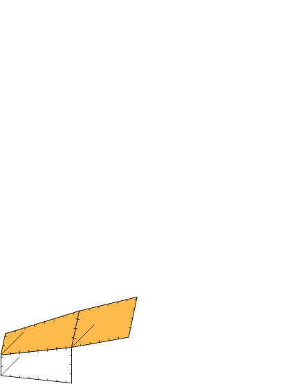
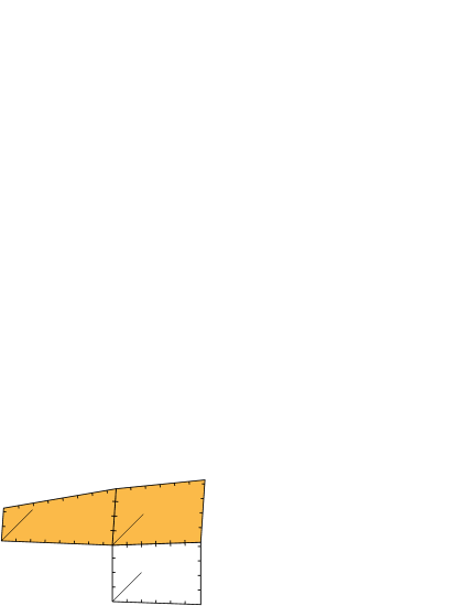
Figure 12: Transfer double sectors. (a) For the left column of the sector model of figure 9, (b) for the right column.

4 Conclusions and outlook

4.1 Summary and pedagogical comments

In this contribution we have shown how paths of light and free particles can be constructed on spacetime sector models. The construction of null geodesics directly leads to the phenomenon of gravitational redshift (section 2.1). The construction of timelike geodesics shows that describing the motion of a particle in free fall as a geodesic in spacetime, provides the expected up-and-down motion in space (section 3.2). By studying timelike geodesics of neighbouring particles, the connection between spacetime curvature and Newtonian tidal forces is revealed (section 3.3).

In connection with the use of spacetime sector models one can discuss the equivalence principle that is expressed here in a clear way. It states that in sufficiently small regions of a curved spacetime Minkowski geometry applies and that locally all physical phenomena are described by the special theory of relativity. In a sector model each sector constitutes such a small region. The curved spacetime is explicitly made up of local regions with Minkowski geometry. In the sector model one can advance through curved spacetime by passing from one Minkowski sector to the next. The local validity of special relativity is directly implemented on sector models, when the world lines of light and free particles are drawn as straight line segments within a sector.

The sector model used here represents a 1+1-dimensional subspace of the Schwarzschild spacetime. It allows the construction of radial world lines. Non-radial world lines can in principle be determined in a 2+1-dimensional sector model, but an implementation with models made from paper or cardboard does not appear practicable. An implementation using three-dimensional interactive computer visualization is being studied.

The workshops on redshift and particle paths presented here were developed and tested at Hildesheim University in the context of an introduction to general relativity for pre-service physics teachers (Zahn and Kraus 2013, Kraus et al 2018). This introductory course uses the model-based approach described here including the calculation of the relevant sector models from their metrics. The calculation of sector models is introduced step by step starting with the sphere via the equatorial plane of a black hole (paper II, section 2.4) to the spacetime of a radial ray (section 2.2). The course uses the material described in papers I to III plus material from part four currently in preparation. In the homework problems and the tutorials, the students calculate sector models for other metrics on their own and use them to study curvature and geodesics. Thus, in the model-based course students are taught the necessary skills for studying (to a certain extent) the physical phenomena associated with a given metric. Answers are here obtained graphically that in a standard university course would be found by calculations. An example of a problem that can be solved with the methods of the model-based course is the following: ‘The metric of a radial ray in an expanding spacetime is given as $\mathrm{d}s^{2}=-c^{2}\mathrm{d}t^{2}+(t/T_{0})^{2}\,\mathrm{d}x^{2}$, where $T_{0}$ is a constant. Two observers, each at a constant coordinate $x$, exchange light signals. Will they observe a redshift?’ Details on the pre-service teacher course and its evaluation are presented by Kraus et al (2018).

Other possible uses, e.g. in an astronomy club at school, exist, in particular, for the workshop on redshift because it does not require the participants to have knowledge of special relativity. Also, all of the material can be used as a supplement to a mathematically oriented university course and help to strengthen geometric insight.

4.2 Comparison with other graphic approaches

Sector models provide a graphic representation of spacetime geodesics. Other graphic representations of geodesics in spacetime have been described using embedding surfaces (Marolf 1999, Jonsson 2001, 2005). Just as the sector models presented here, these representations are limited to 1+1-dimensional spacetimes. A related representation of geodesics is the construction on so-called wedge maps developed by diSessa (1981). This construction is derived from the Regge calculus and is carried out numerically. The calculation is also described for 2+1-dimensional spacetimes; light deflection and redshift are discussed.

In comparison to embedding surfaces and also to wedge maps, the calculation and use of sector models is more elementary. For a spacetime model, only a basic knowledge of special relativity is necessary; the determination of geodesics is carried out graphically and the only mathematical concept that goes beyond elementary mathematics as taught at school is the concept of the metric. Sector models can easily be constructed and since they are readily duplicated, all participants of a course can carry out the construction of geodesics themselves on their own models.

4.3 Outlook

In the model-based approach described here, sector models are the basis for answers to the three fundamental questions raised in paper I concerning the nature of a curved spacetime, the laws of motion, and the relation between the distribution of matter and the curvature of spacetime. In paper I curved spaces and spacetimes are represented as sector models. In paper II and the present contribution geodesics are studied as paths of light and free particles. Part four of this series will be on the relation between curvature and the distribution of matter.

References

- (1)
- diSessa (1981) diSessa A 1981 An elementary formalism for general relativity Am. J. Phys. 49 (5) 401–11
- Jonsson (2001) Jonsson R M 2001 Embedding spacetime via a geodesically equivalent metric of euclidean signature Gen. Rel. Grav. 33 (7) 1207–35
- Jonsson (2005) Jonsson R M 2005 Visualizing curved spacetime Am. J. Phys. 73 (3) 248–60
- Kraus et al (2018) Kraus U, Zahn C, Reiber T and Preiß S 2018 A model-based general relativity course for physics teachers, submitted
-
Kraus and Zahn (2018)
Kraus U and Zahn C 2018
Online resources for this contribution
www.spacetimetravel.org/sectormodels3 - Marolf (1999) Marolf D 1999 Spacetime embedding diagrams for black holes Gen. Rel. Grav. 31 (6) 919–44
- Regge (1961) Regge T 1961 General relativity without coordinates Il Nuovo Cimento 19 558–71
- Williams and Ellis (1981) Williams R M and Ellis G F R 1981 Regge Calculus and Observations. I. Formalism and Applications to Radial Motion and Circular Orbits Gen. Rel. Grav. 13 (4) 361–95
- Zahn and Kraus (2013) Zahn C and Kraus U 2013 Bewegung im Gravitationsfeld in der Allgemeinen Relativitätstheorie – ein neuer Zugang auf Schulniveau PhyDid B DD 17.13
-
Zahn and Kraus (2014)
Zahn C and Kraus U 2014