The $\gamma$-ray emitting region in low synchrotron peak blazars

Abstract

Aims. From the early days in $\gamma$-ray astronomy, locating the origin of GeV emission within the core of an active galactic nucleus (AGN) persisted as an open question; the problem is to discern between near- and far-site scenarios with respect to the distance from the super massive central engine. We investigate this question under the light of a complete sample of low synchrotron peak (LSP) blazars which is fully characterized along many decades in the electromagnetic spectrum, from radio up to tens of GeV. We consider the high-energy emission from bright radio blazars and test for synchrotron self-Compton (SSC) and external Compton (EC) scenarios in the framework of localizing the $\gamma$-ray emission sites. Given that the inverse Compton (IC) process under the EC regime is driven by the abundance of external seed photons, these photons could be mainly ultraviolet (UV) to X-rays coming from the accretion disk region and the broad-line region (BLR), therefore close to the jet launch base; or infrared (IR) seed photons from the dust torus and molecular cloud spine-sheath, therefore far from jet launch base. We investigate both scenarios, and try to reveal the physics behind the production of $\gamma$-ray radiation in AGNs which is crucial in order to locate the production site.

Methods. Based on a complete sample of 104 radio-selected LSP blazars, with 37 GHz flux density higher than 1 Jy, we study broadband population properties associated with the nonthermal jet emission process, and test the capability of SSC and EC scenarios to explain the overall spectral energy distribution (SED) features. We use SEDs well characterized from radio to $\gamma$ rays, considering all currently available data. The enhanced available information from recent works allows us to refine the study of Syn to IC peak correlations, which points to a particular $\gamma$-ray emission site.

Results. We show that SSC alone is not enough to account for the observed SEDs. Our analysis favors an EC scenario under the Thomson scattering regime, with a dominant IR external photon field. Therefore, the far-site (i.e., far from the jet launch) is probably the most reasonable scenario to account for the population properties of bright LSP blazars in cases modeled with a pure leptonic component. We calculate the photon energy density associated with the external field at the jet comoving frame to be $\rm U^{\prime}_{ext}=1.69\times 10^{-2}$ erg/cm³, finding good agreement to other correlated works.

1 Introduction

Locating the emission site where MeV-TeV photons are produced in active galactic nuclei (AGNs) has been as an open question since the early days of $\gamma$-ray astronomy (Vovk & Neronov, 2013; Neronov et al., 2015); one of major limitations is the angular resolution of the current generation of satellite-borne MeV-GeV and ground-based GeV-TeV observatories. Currently, we do not have enough resolution to distinguish $\gamma$-ray substructures within the jets, even for close-by objects. The main class of AGNs detected from MeV up to tens of TeV are called blazars, and usually show extreme properties like high-power output together with short timescale variability (Aharonian et al., 2007), which are the main focus of studies trying to localize the $\gamma$-ray emission site.

In summary, blazars are a particular class of jetted AGNs corresponding to the very few cases where the jet is pointing close to our line of sight (Padovani et al., 2017). They are known to have a unique spectral energy distribution (SED) often characterized by the presence of two nonthermal bumps in the log($\nu$f_ν) versus log($\nu$) plane, extending along the whole electromagnetic window, from radio up to TeV $\gamma$ rays. Blazars are also known for their rapid and high-amplitude spectral variability. Usually, the observed radiation shows extreme properties owing to the relativistic nature of the jets, which result in amplification effects. Those objects are relatively rare. Only $\sim$ 4000 cases have been optically identified since the latest blazar surveys, 5BZcat Massaro et al. (2015) and 2WHSP Chang et al. (2017), and have been extensively studied by means of a multifrequency approach, which has cumulated impressive dedicated databases at radio, microwave, infrared (IR), optical, ultraviolet (UV), X-ray, and $\gamma$ rays.

According to the standard picture (e.g., Giommi et al., 2012a), the first peak in the log($\nu$f_ν) versus log($\nu$) plane is associated with the emission of synchrotron (Syn) radiation owing to relativistic electrons moving through the jet’s collimated magnetic field. The second peak is usually described as a result of inverse Compton (IC) scattering of low-energy photons to the highest energies by the same relativistic electron population that generates the Syn photons (synchrotron self-Compton model, SSC). The seed photons undergoing IC scattering can also come from outside regions (external Compton models, EC), like the accretion disk, the broad-line region (BLR), the dust torus, and even from illuminated molecular clouds, adding extra ingredients for modeling the observed SED.

Since the peak-power associated with the synchrotron bump tell us at which frequency ($\rm\nu_{peak}^{Syn}$) most of the AGN electromagnetic power is being released, the parameter log($\nu_{peak}^{Syn}$) has been extensively used to classify blazars. Following discussion from Padovani & Giommi (1995) and Abdo et al. (2010a), objects with $\rm log(\nu_{peak}^{Syn})<14.5$, between 14.5 and 15.0, and $>$ 15.0 [Hz] are respectively called low, intermediate, and high synchrotron peak (LSP, ISP, HSP) blazars. Some blazars whose Syn peaks reach the hard X-ray band are called extreme HSP (EHSP) blazars; moreover, evidence for Syn peak at the MeV–GeV range are still under debate, with several cases of EHSP blazars already being studied, for example in Chang et al. (2017); Kaufmann et al. (2011); Tavecchio et al. (2011); Tanaka et al. (2014) and Arsioli et al. (2018). EHSP blazars are not easy to identify as they are typically faint in radio and hardly detected by current radio sky surveys; moreover, there is increasing attention from the physics community given the possibility that blazars might be associated with astrophysical neutrinos (Padovani et al., 2016, 2018) and with ultra-high-energy cosmic rays (Resconi et al., 2017). Given the broad context in which blazars play an important role for the future of astroparticle physics, studying the production site of $\gamma$ rays for the subsample of LSP blazars may bring relevant elements for the understanding of high and very high-energy mechanisms in action for the entire blazar population.

From current leptonic-based models, synchrotron photons and external thermal photons interacting with relativistic particles in the jet may be scattered to much higher energies, characterizing the inverse Compton (IC) process. A simple treatment can show how this process works. In the electron frame $l^{\prime}$, the synchrotron photons moving along with electrons will appear to have much lower energy, $h\nu_{1}^{\prime}\ll m_{e}c^{2}$. In the laboratory (astrophysical source) frame $l$, the relativistic Doppler shift formula is given by

$$\rm h\nu_{1}^{\prime}=\gamma h\nu_{1}\big{(}1+\beta\cos\theta\big{)}\,,$$ (1)

where $\rm\theta$ is the angle between the propagation direction of photons and electrons, $\rm\gamma=1/\sqrt[]{1-\beta^{2}}$ represents the Lorentz factor for the relativistic electron, and $\beta=v/c$. In the electron comoving frame $l^{\prime}$, this angle seems much smaller $\rm sin\theta^{\prime}=\frac{\sin\theta}{\gamma(1+\beta\cos\theta)}$ so that all photons will appear to approach in head-on collision, and Eq. 1 reduces to $\rm h\nu_{1}^{\prime}\approx\gamma h\nu_{1}\big{(}1+\beta\big{)}$, since $\rm\theta\ll 1$. Also, in $l^{\prime}$ frame the photon energy seems much lower ($\rm h\nu^{\prime}\ll m_{e}c^{2}$) and the interaction can be treated as elastic Thomson scattering. Therefore, in $l^{\prime}$ frame the photon energy does not change much during the collision $\rm E_{1}^{\prime}\approx E_{2}^{\prime}$ and $\rm\nu_{1}^{\prime}\approx\nu_{2}^{\prime}$. In the AGN source frame $l$, however, photons are scattered along the direction of the relativistic electrons with $\rm\nu_{2}=\delta\nu_{2}^{\prime}\approx\delta\nu_{1}^{\prime}$, where $\rm\delta^{-1}=\gamma\big{(}1+\beta\cos\theta\big{)}$ is the beaming factor, which reduces to $\rm\delta^{-1}\approx\gamma\big{(}1+\beta\big{)}$ so that we have $\rm\nu_{2}=\nu_{1}\big{[}\gamma\big{(}1+\beta\big{)}]^{2}$. In the relativistic limit, $\rm\beta\approx 1$, and the frequency associated with the upscattered photon follows as $\rm\nu_{2}\approx 4\ \gamma^{2}\ \nu_{1}$.

Therefore, an important conclusion is that photons scattered by relativistic electrons gain energy with a $\rm\gamma^{2}$ factor: $\rm E_{2}\propto\gamma^{2}E_{1}$. Naturally, the luminosity $\rm L_{IC}$ of the inverse Compton component depends on the photon density $n_{ph}$ available for up-scattering via the IC process. In the SSC model only photons generated by the synchrotron process itself may build up the available $n_{ph}$. In addition, the external contribution from thermal emission regions can be significant sources of low-energy photons, characterizing the EC models. In both cases we have $\rm L_{IC}\propto n_{ph}\gamma^{2}E_{1}$ (Rybicki & Lightman, 1986).

As is known, the synchrotron emission can extend up to hard X-rays, and in some extreme cases can even peak in this region. When the photon energy reaches a level that is similar to the electron mass, the condition $h\nu^{\prime}\ll mc^{2}$ is not valid in the electron’s frame, and Klein–Nishina effect (described by applying quantum electrodynamics to the scattering process) acts to reduce the electron-photon cross section with respect to the case of classical Thomson scattering ($\sigma_{T}$). Therefore, the IC scattering might becomes less and less efficient for seed photons with the highest energies (e.g., $\rm\sigma_{KN}/\sigma_{T}\approx 0.5$ at E = 300 KeV), which influence the spectral energy distribution of blazars at very high energies E $>$ 100 GeV and manifest as a strong break (steepening) in $\gamma$-ray emitted power. In fact, if the electron energy distribution follows $\rm N_{(E)}=kE^{-p}$, the scattered IC spectrum will also be a power law with spectral index $\rm\alpha=(1-p)/2$.

Although a pure leptonic IC process is well established as the mechanism that produce the second bump observed on the blazar’s SED, there is still open debate on alternative scenarios like the ones considering hadronic plus leptonic components (Böttcher et al., 2013; Cerruti et al., 2015, 2017b). In addition, the location and AGN environment dependences associated with the production of $\gamma$ rays are still unclear. Probing such information demands a set of multifrequency measurements together with model-dependent tests, as we discuss below. Given the many identified $\gamma$-ray sources, there is still a great deal of room to explore issues like variability (comparing the behavior at low and high energies) and probing the far end of SED at E $>$ 10 TeV with the upcoming generation of Cherenkov telescope arrays (CTA, Bernlöhr et al., 2013).

In this work we focus on modeling low synchrotron peak (LSP) blazars making use of a complete sample of radio-loud blazar AGNs described in details by Planck Collaboration et al. (2011). It consists of 104 northern and equatorial sources with declination greater then -10^o, flux density at 37 GHz exceeding 1 Jy as measured with the Metsähovi radio telescope. All 104 sources have been detected between 30 GHz and 857 GHz by the Planck mission (Planck Catalogue of Compact Sources PCCS, Planck Collaboration et al., 2014a) most of which were previously known. With the addition of PCCS data, many radio-bright blazars gained a better multifrequency description for their synchrotron (Syn) component, and here are referred to as radio-Planck sources.

It is important to note that the vast majority of these sources (103) are legitimate LSP blazars (two cases at the border line, $\nu_{peak}\approx$10^14.5 Hz, BZQJ 0010+1058 and BZBJ 0050-0929); only one bright HSP blazar (BZBJ 1653+3945) was removed or properly highlighted during the preparation of following studies. Out of those 104 sources, 83 have a confirmed $\gamma$-ray counterpart in at least one of the Fermi-LAT (Atwood et al., 2009) catalogs 1FGL, 2FGL, and 3FGL (Abdo et al., 2010b; Ackermann et al., 2011; Acero et al., 2015) and another 16 had their $\gamma$-ray spectrum recently described by Arsioli & Polenta (2018), who search for new $\gamma$-ray emitting blazars following the same approach as Arsioli & Chang (2017). We note that their study was based on a dedicated Fermi-LAT analysis showing that many of the previously $\gamma$-ray undetected LSPs are actually detectable when integrating over 7.5 years of observations.

The online SED builder tool was used in previous work to compile and fit all available multifrequency data (Arsioli & Polenta, 2018) that we now use for current analysis. This included relevant microwave flux measurements coming from the Planck mission, the new $\gamma$-ray data-points from the Fermi-LAT dedicated analysis, and extra UV to X-ray observations from Swift. From there, fitting parameters were extracted to describe the observed peak-frequency log($\nu_{peak}$) and peak-brightness log($\nu$f_ν) for both Syn and IC bumps. We now use those measurements to gain further insight on the population properties of LSP blazars, calculating parameters like the Lorentz factor associated with relativistic electrons in the jet, the product B$\delta$ ($\delta$ stands for the beaming factor), the luminosity associated with Syn and IC peaks, and the external photon field energy density (U_ext) calculated when assuming an EC models.

2 LSPs jets and nonthermal emission mechanism

As argued in the literature (Paliya et al., 2017; Lister et al., 2015) LSP blazars with $\rm\nu_{peak}<10^{13.4}$Hz may show a typical inverse Compton peak below 0.1 GeV, and thus out of the Fermi-LAT sensitivity bandwidth at 0.1–500 GeV. In the case of LSP blazars, we might probe only the very end of the IC component, and this is why a considerable percentage of LSPs ($\sim$20%) had no counterpart in the latest Fermi-LAT catalogs (1FGL, 2FGL, and 3FGL). The relation between Syn and IC peaks is explored in Abdo et al. (2010a); Gao et al. (2011); Zhang et al. (2012), with Şentürk et al. (2013) showing a correlation between peak frequencies, since $\nu^{IC}_{peak}$ is decreasing with respect to HBL-LBL-FSRQ. There is a clear connection between the distributions of $\rm log(\nu^{Syn}_{peak})$ and $\rm log(\nu^{IC}_{peak})$ when a complete sample of LSPs is considered, such that a characteristic peak ratio ($\rm PR=log(\nu^{IC}_{peak}/\nu^{Syn}_{peak})$ is very suitable for describing the average relation between their distributions ($\rm PR\approx 8.6$, Arsioli & Polenta, 2018). However, when taken case by case, they show that an intrinsic and direct relation between peak frequencies is nontrivial and most probably highly dependent on its SSC or EC dominance nature and variability.

Intrinsic jet properties like the beaming factor ($\delta$) and the dominant IC regime (either synchrotron self-Compton, SSC, or external Compton, EC) may in fact have a strong influence on the $\gamma$-ray variability, and also affect the Fermi-LAT detectability of a few radio-loud blazars. Lister et al. (2009) have shown that the $\gamma$-ray sources detected during the first three months of Fermi-LAT operations are on average the ones associated with the highest apparent jet speeds (based on radio measurements with the Very Large Baseline Array, VLBA) and therefore the most powerful accelerators with the highest $\rm\delta$ values.

In a simple SSC scenario (Maraschi et al., 1992; Marscher & Travis, 1996) the intensity boosting factor scales as $\delta^{3+\alpha}$, where $\alpha$ is the spectral index given that the flux scales as S${}_{\nu}\propto\nu^{-\alpha}$. When considering typical blazar SEDs in the S_ν versus $\nu$ plane, the spectrum tends to be flat at radio frequencies and steep in $\gamma$ rays. As a consequence, the intensity boosting is more pronounced in $\gamma$ rays than in the radio bands, and thus the $\gamma$-ray detection of faint sources is favored during flaring episodes.

Considering the mechanism involved for the IC scattering, additional photon fields could be present and even dominant with respect to synchrotron photons (Dermer, 1995; Jones et al., 1974). For instance, the jet might interact with external photons produced by the accretion disk, reflections, and IR thermal emission from surrounding gas clouds and dust torus. In such scenarios, a considerable amount of the $\gamma$-ray emission would be produced by Compton scattering of those external photons which is associated with an additional boosting factor $\delta^{1+\alpha}$ enhancing the IC intensity.

Given that nearly all radio-Planck sources are now well described in $\gamma$ rays, we study their population properties to probe the leading emission mechanism, either SSC or EC, looking for hints to locate the $\gamma$-ray emitting region in LSP blazars.

3 Comments on synchrotron self-Compton and external Compton scenarios

Identifying the dominant IC mechanism can help to locate the $\gamma$-ray emitting region and to better understand its underlying physics. If the IC emission is dominated by EC process and happens close to the black hole (0.1–1 pc distance, embedded in the BLR) it could explain the observed $\gamma$-ray short timescale variability of a few hours (Aharonian et al., 2007; Pittori et al., 2018). In this case, since optical-UV BLR photons would be available for up-scattering, there should be a strong correlation between $\gamma$-ray and optical-UV flares. However, an alternative scenario considers that the $\gamma$-ray emission originates farther from the black hole (BH) at distance $\gg$1 pc. In this case, an IR photon field generated by the molecular clouds and dust torus (through reprocessing radiation from the accretion disk, or even by illumination from the jet synchrotron emission itself) are possible dominant sources of seed photons for up-scattering to higher energies (Breiding et al., 2018).

Both SSC and EC scenarios with $\gamma$ rays originating far from the BH (out of the BLR region) demands that the jet structure should be a very narrow opening ($\approx$0.8 pc scale) or have N substructures ($\approx$0.8/$\sqrt{N}$ pc), as invoked by multicomponent scenarios, to reconcile with the short timescale variability observed in the GeV–TeV band (Agudo et al., 2011).

There are indeed plenty of arguments supporting the far-site emission. One is related to radio-mm observations with the Very Long Baseline Array (VLBA) which shows radio-mm variability (at a distance on the order of   12–14 pc from the BH, for the BL Lac AO 0235+164 and OJ 287, Agudo et al., 2011, 2013) to be correlated in time with $\gamma$-ray flares, and therefore supposed to happen in the same site. If this is true, there remains the question of how all the power gets transferred so efficiently farther away from the BH to produce the VHE component we observe. In addition, BL Lacs are usually dominated by nonthermal emission along the whole spectrum, with no trace of disk or dust torus thermal component.

Agudo et al. (2013) has interpreted the far emission site for BL Lacs AO 0235+164 and OJ 287 in the framework of SSC scenario since no other evident photon field is present for up-scattering other then the nonthermal synchrotron photons. However, similar work from Ackermann et al. (2012) for the same object and flaring event (AO 0235+164, 2008) describes the IC component within an EC scenario, assuming the external photon field is dominate by IR photons from the surrounding dust torus, which are up-scattered to HE. An extra IR component could also be present and dominant as a consequence of illumination and sublimation of the molecular cloud (MC) torus in a spine-sheath geometry as described by Breiding et al. (2018) and MacDonald et al. (2015). We should not avoid mentioning several works, such as Nalewajko et al. (2014) and Neronov et al. (2015) in favor of a close-site emission at the vicinity of the AGN supermassive black hole.

Even though we do not have evidence of MC or dust torus thermal components in BL Lacs, we should note that the nonthermal jet synchrotron emission is beamed and dominant because our observer frame is watching a relativistic jet pointing close to our line of sight. Thermal components from the MC and dust torus could well be present, nevertheless swamped by the jet beamed emission. Given the relativistic nature of the jet, even a relatively faint photon field with energy density $\rm U_{ext}$ would be boosted in the jet’s “$\prime$” reference frame $\rm U^{\prime}_{ext}\propto U_{ext}\Gamma^{2}$ (Ghisellini & Madau, 1996). This could become much more relevant or even dominant with respect to the Syn photon field produced by the jet itself, and strongly depending on the Lorentz factor ($\Gamma$).

The discussion surrounding the $\gamma$-ray emitting region in AGNs is ample, and interpretations are always subject to multiple free parameters that can be fine-tuned for different scenarios. We try to contribute to that understanding by studying general properties of the radio-Planck sample as a fair representation of powerful LSP blazars.

4 Lorentz factor of jet’s relativistic electrons

Assuming a homogeneous SSC to describe the blazar SED, high-energy photons are generated by the up-scattering of low-energy Syn photons due to their interaction with relativistic electrons from the jet. In this scenario, a single population of relativistic electrons is then responsible for the entire SED, resulting in a strong correlation between the Lorentz factor of the electrons $\rm\gamma_{peak}$ emitting at the peak of the Syn component, and the peak frequency from the Syn and IC components:

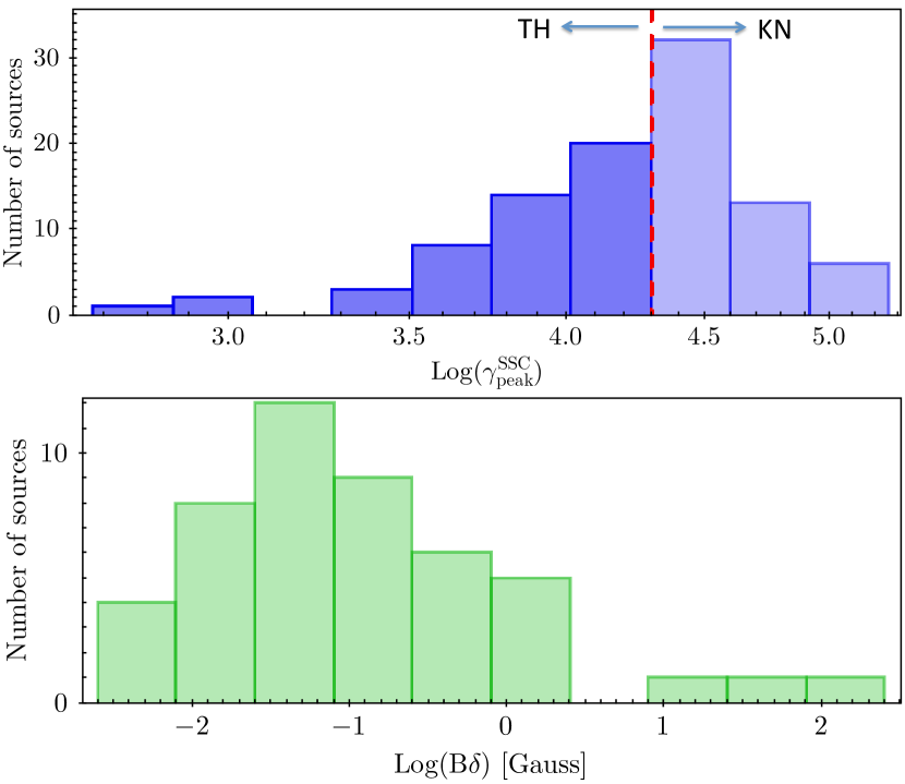
Figure 1: Top: Distribution of Lorentz factor $\rm\gamma^{SSC}_{peak}$ for electrons emitting in the peak of the Syn component (eq. 2). The red dashed line shows the limit for $\rm\gamma^{SSC}_{peak}$ values where the transition from TH to KN scattering regime occurs. Bottom: Distribution of the $\rm B\delta$ parameter for LSP sources assuming a SSC model, and considering only sources with $\rm\gamma^{SSC}_{peak}<2\times 10^{4}$ (under TH regime).

$$\gamma_{peak}\simeq\sqrt{3/4\times\nu^{IC}_{peak}/\nu^{Syn}_{peak}}\$$ (2)

However, this trend is valid only under Thomson regime (TH) of the IC scattering, that is for $\rm\gamma_{peak}<2\times 10^{4}$, where the transition to the Klein–Nishina (KN) regime occurs. We use eq. 2 to calculate $\rm\gamma^{SSC}_{peak}$ for all 99 sources with Syn and IC parameters available (Table The $\gamma$-ray emitting region in low synchrotron peak blazars), and plot its distribution in fig. 1, top. The histogram shows a Gaussian distribution with slightly negative skewness, and characterized by mean $\rm\langle log(\gamma^{SSC}_{peak})\rangle=4.24\pm 0.05$. Therefore, half of the sample have $\rm\gamma^{SSC}_{peak}>2\times 10^{4}$, which is in tension with the fact that we are dealing with bright LSPs. Apart from a single HSP (Mrk501), all sources have $\rm\nu^{Syn}_{peak}<10^{14.6}$ Hz and the transition from TH to KN regime is only expected for $\rm\nu^{Syn}_{peak}>10^{14.7}$ Hz in the case of a single-zone SSC model.

In a simple single-zone self-synchrotron model, the $\rm\nu^{Syn}_{peak}$ can be written in terms of jet magnetic field (B), beaming factor ($\delta$), and peak Lorentz factor ($\rm\gamma_{peak}$). As discussed in Abdo et al. (2010a), assuming an emitting region of size R$\sim$10¹⁵cm, and a log-parabola to describe the distribution of Lorentz factor: $\rm n_{(\gamma)}\,=\,k\times 10^{r\ log(\gamma/\gamma_{peak})^{2}}$ (curvature parameter r = 2.0, $\gamma$ ranging from 10² to 6$\times$10⁵, and electron density of $\rm\sim 1.0\,cm^{-3}$; Tramacere et al. 2010), we have

$$\nu^{Syn}_{peak}=3.2\times 10^{6}(\gamma_{peak})^{2}B\delta/(z+1)\ ,$$ (3)

which is valid up to $\rm\nu^{Syn}_{peak}\approx 10^{14.7}$ Hz, where the transition to KN scattering regime occurs. Following the discussion from Abdo et al. (2010a), $\rm\gamma^{SSC}_{peak}\approx\gamma_{peak}$ under TH regime, therefore we use eq. 3 to calculate the B$\delta$ parameter as B$\rm\delta=\nu^{Syn}_{peak}(1+z)/(3.2\times 10^{6}\times(\gamma^{SSC}_{peak})^{2}$), only for the subsample of 48 sources having $\rm\gamma^{SSC}_{peak}<2\times 10^{4}$. These 48 sources are the ones under TH regime if we assume a single-zone SSC model. We plot the B$\delta$ distribution in Fig. 1 (bottom) which peaks at $\langle B\delta\rangle$=0.066${}^{+0.020}_{-0.015}$ gauss. This is also in tension with the expected value for the B$\delta$ parameter for blazars, which is usually assumed to be $\rm\langle B\delta\rangle_{expected}=10$ gauss, with beaming factor $\delta$ on the order of $\sim$20 (ranging from 5 to 35 for LSP blazars, Kang et al., 2014) and B on the order of $\sim$0.5 gauss (ranging from 0.3 to 1.5 gauss, Tramacere et al., 2010). Most probably, the $\gamma^{SSC}_{peak}$ values that we have calculated from eq. 2 are highly overestimated, leading to low B$\delta$ values. Therefore a simple single-zone SSC model seems insufficient to account for the overall SEDs observed for LSP blazars.

4.1 Tramacere plane: log($\gamma^{SSC}_{peak}$) versus log($\nu^{Syn}_{peak}$)

Tramacere et al. (2010) proposes the use of the log($\gamma^{SSC}_{peak}$) versus log($\nu^{Syn}_{peak}$) plane to better understand the dominant emission mechanism in blazars (either SSC or EC) for individual sources and populations, as also mention by Abdo et al. (2010a). In fig. 2 we show the radio-Planck sources in this plane, with $\rm\gamma^{SSC}_{peak}$ values estimated using eq. 2, directly from the Syn and IC peak-power parameters measured from fitting the SEDs case by case (Table The $\gamma$-ray emitting region in low synchrotron peak blazars).

In this plane, the blue dashed line (extracted from Tramacere et al. 2010, their Fig. 3) represents a SSC numerical model which incorporates the TH to KN transition, and therefore corrects for the decreasing e^-+$\gamma$ cross-section which reduces the efficiency of IC scattering and affects the cooling time of relativistic electrons in the jet. The black dashed line represents the synchrotron emission, simply plotting eq. 3 for the SSC model with no correction on the TH to KN transition (assuming R$\sim$10¹⁵cm and B$\delta$/(1+z)=1.3 to match with the SSC-TH estimate from the numerical modeling). The purple dashed line (Tramacere et al. (2010), also from their Fig. 3) represents a numerical model for the EC regime assuming benchmark values for the jet parameters: R$\sim$10¹⁵cm, a log-parabola to describe the distribution of Lorentz factor ($\gamma$) of the jet’s relativistic electron, assuming a dominant UV external photon field produced by the accretion disk (modeled as a blackbody with T profile having innermost T of $\approx$10⁵ K), and assuming an extra component reflected by the BLR toward the jet, with efficiency $\tau$=10%. Those models are described and applied in a series of works: Tramacere & Tosti (2003); Massaro et al. (2006); Tramacere (2007); Tramacere et al. (2009).

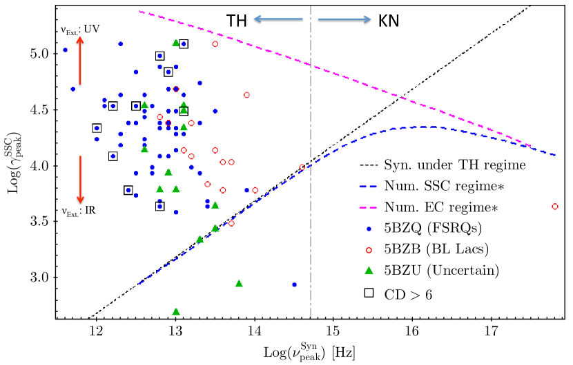
Figure 2: The $\rm log(\gamma^{SSC}_{peak})$ vs. $\rm log(\nu^{Syn}_{peak})$ plane. Sources are divided according to their classification in the 5BZcat: blue circles for 5BZQs (FSRQ), red empty circles for 5BZBs (BL Lacs), and green triangles for 5BZUs (unclassified). Blue and purple dashed lines correspond to $\gamma^{SSC}_{peak}$ calculated from numerical simulations considering SSC and EC scenarios incorporating the transition from TH and KN regimes. The vertical dot-dashed line indicates the $\nu^{Syn}$ domains for which TH and KN regimes apply. The black dashed line represents eq. 3 using B$\delta$/(1+z)$\approx$1.3 gauss, with no correction for the TH to KN transition.

We separate sources according to their classification in the 5BZcat catalog (BZBs, BZQs, Uncertain types, Massaro et al. (2015)), and also mark cases with the highest Compton Dominance (CD) values (CD $>$ 6.0 to select the top 10% of sources). Most sources cluster in the region above the blue dashed line, meaning they are mainly out of the SSC domain. This region is characteristic of blazars where there might be an external photon field ranging from IR to UV playing an important role.

In conclusion, an EC mechanism under the TH scattering regime should be more suitable to study those sources. The Tramacere plane then gave us an overview on the dominant IC mechanism in play for bright LSP blazars, and also shows that there is no significant differences (data clustering) with respect to the $\gamma^{SSC}_{peak}$ parameter depending on blazar type or Compton dominance.

4.2 Assuming a dominant EC scenario

If we assume that a source can be described via the EC model under the TH regime, the frequency associated with the IC peak ($\rm\nu^{EC}_{peak}$) should be well described by (Abdo et al., 2010a)

$$\rm\frac{\nu^{EC}_{peak}}{\nu^{ext}_{peak}\Gamma}=\frac{4}{3}\big{(}\gamma_{peak}\big{)}^{2}\frac{\delta}{(1+z)},$$ (4)

where $\gamma_{peak}$ is the Lorentz factor associated with jet electrons emitting in the peak of the synchrotron component (see eq. 2) and $\rm\nu^{ext}_{peak}$ is the peak frequency associated with the external photon field in the rest frame from the emitting zone (either accretion disk, BLR, MC, or dust torus). When $\rm\nu^{ext}_{peak}$ is multiplied by the bulk Lorentz factor $\Gamma$ associated with the relativistic outflow, it transforms this frequency to the jet rest frame. We use the notation $\rm\gamma^{EC}_{peak}$ to represent $\rm\gamma_{peak}$ when assuming an EC scenario.

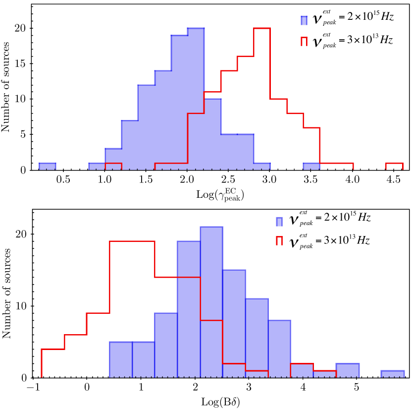
Figure 3: Top: Distribution of $\rm log(\gamma^{EC}_{peak})$ for the radio-Planck sample based on eq. 4 when assuming $\rm\Gamma=20$, and for two different external photon fields: dust torus photons peaking at IR $\rm\nu^{ext}_{IR}=3\times 10^{13}Hz$ (in red); near-UV photons from the BLR region, peaking close to $\rm Ly_{\alpha}$, $\rm\nu^{ext}_{UV}=2\times 10^{15}Hz$ (full indigo bars). Bottom: Corresponding distribution of $\rm log(B\delta$) calculated from eq. 3 for $\rm\gamma_{peak}=\gamma^{EC}_{peak}$, and considering $\nu^{Syn}_{peak}$ and $\nu^{IC}_{peak}$ from Table The $\gamma$-ray emitting region in low synchrotron peak blazars.

We use eq. 3 to calculate $\rm\gamma^{EC}_{peak}$ for all sources with available IC data, considering $\rm\nu^{IC}_{peak}$ ($\rm\equiv\nu^{EC}_{peak}$) as reported in Table The $\gamma$-ray emitting region in low synchrotron peak blazars. To perform this calculation we assume the Doppler (beaming) factor $\rm\delta=[\Gamma(1-\beta cos\theta)]^{-1}\approx\Gamma$ (Dermer, 2015) valid for sources observed close to the line of sight, $\rm\theta<5^{\circ}$.

We assume $\langle\delta\rangle$$\approx$ 20$\pm$2, following Kang et al. (2014), which presents a list of $\delta$ parameter for 15 bright LSPs, as estimated from the model constrained by SED fitting and in agreement with estimates from radio variability and brightness temperature (confirming early measurements made by Jorstad et al. (2005)). Also, Saikia et al. (2016) introduced a new independent method based on the optical fundamental plane of black hole activity to estimate the $\Gamma$ distribution, showing a valid range from 1 to 40, with N${}_{(\Gamma)}\propto\Gamma^{-2.1\pm 0.4}$, or an even more restrictive range with $\Gamma$ between 15 and 30 (Nalewajko et al., 2014), as deduced from a study of $\gamma$-ray flares, with a multifrequency approach and testing EC scenarios.

There are two different setups that are important to consider, and that are related to the photon-frequency ($\nu$) associated with the external photon field. The first one assumes that seed photons originate mainly from the dust torus. This view is supported by Cleary et al. (2007) who deduced from observations with Spitzer that the torus may heat up to 150–200 K by absorbing accretion disk radiation and emitting like a blackbody, and therefore with dominant IR emission peaking at $\rm\nu^{ext}_{IR}=3\times 10^{13}Hz$. There is a similar scenario where the illumination and sublimation of molecular clouds, owing to synchrotron jet emission in a spine-sheath geometry (Breiding et al., 2018), could also play important role in producing a dominant IR photon field. In the second setup the external photon field originates from the BLR and accretion disk regions, with dominant emission peaking close to Ly_α in near UV, at $\rm\nu^{ext}_{UV}=2.0\times 10^{15}Hz$ (Tavecchio & Ghisellini, 2008; Ghisellini & Tavecchio, 2008).

In Fig. 3 (top) we plot the distribution of $\rm log(\gamma^{EC}_{p})$ for the radio-Planck sample, which leads us to the following conclusion. When using an EC model with external photon field ranging from UV to IR, and assuming $\langle\delta\rangle\approx\langle\Gamma\rangle$ = 20, almost all sources are under the TH scattering regime. This is in agreement with expectations since the radio-Planck sample is dominated by LSP blazars, $\rm\nu^{Syn}_{peak}<10^{14}$ Hz. We find $\rm\langle log(\gamma^{EC}_{peak})\rangle$ ranging from 2.80$\pm$0.05 to 1.93$\pm$0.05 depending on the external photon field, UV and IR, respectively. Compared to $\gamma^{SSC}_{peak}$ values calculated when assuming a simple SSC model (Fig. 1), we see that $\gamma^{SSC}_{peak}$ is highly overestimated by almost two orders of magnitude in any scenario.

As mention previously, eq. 3 is only valid under the TH regime. Therefore, we recalculate the B$\delta$ parameter according to B$\rm\delta=\nu^{Syn}_{peak}(1+z)/(3.2\times 10^{6}\times(\gamma^{EC}_{peak})^{2}$), which now applies to the subsample of 98 sources having $\rm\gamma^{EC}_{peak}<2\times 10^{4}$. We plot the B$\delta$ distribution in Fig. 3 (bottom), which peaks at $\rm\langle log(B\delta)\rangle=2.72\pm 0.09$ for the UV external field and at $\rm\langle log(B\delta)\rangle=0.99\pm 0.09$ for the IR external field. Therefore, assuming $\rm\langle\delta\rangle=20$ we get an estimate for the magnetic field in the jet $\rm\langle B_{UV}\rangle=26.2$ gauss, and $\rm\langle B_{IR}\rangle=0.48$ gauss. In particular, the estimate for $\rm\langle B_{UV}\rangle$ is not consistent with the constraints from SED fitting when assuming an emission site within the BLR (Cao & Wang, 2013), owing to underestimated $\rm\gamma^{EC}_{peak}$ values. However, the estimate for $\rm\langle B_{IR}\rangle$ is in good agreement with expectations from SED fitting from Kang et al. (2014) for $\gamma$-ray emission out of the BLR region (far-site) at a distance $\gg$ 0.1 pc from the BH.

This suggests that an IR external photon field might be the dominant driver in the EC scenario for the population of bright LSP blazars, also in agreement with findings from Abdo et al. (2015). One important aspect to note is that the energy density (U) from external photon fields are boosted in the jet’s comoving frame “$\prime$” according to $\rm U^{\prime}_{ext}=U_{ext}\Gamma^{2}$ (Sikora et al., 2009), therefore strongly dependent on the jet’s bulk Lorentz factor $\Gamma$ and accounting for $\rm U^{\prime}_{ext}$ being dominant with respect to the self-synchrotron photon field.

If we assume an UV external photon field from the BLR region, forcing the magnetic field to $\rm 0.5<B<2.0$ gauss as expected from SED fitting derived from Cao & Wang (2013), it may lead to highly overestimated $\gamma^{EC}_{peak}$ values, as also reported by Abdo et al. (2010a). In fact, when relaxing the value associated with $\langle\delta\rangle$, it is possible to adjust UV dominant scenarios for some individual sources, and that is a known degeneracy associated with the B$\delta$ parameter.

4.3 Syn versus IC luminosity correlation

We have calculated the Syn and IC peak luminosities based on the flux density $\nu$f_ν [ergs/cm²/s] measurements listed in Table The $\gamma$-ray emitting region in low synchrotron peak blazars. Luminosity is given by

$$\rm L=\frac{4\pi d^{2}_{L}\ \nu f_{\nu}}{(1+z)^{1-\alpha}}\equiv 4\pi d^{2}_{L}\ \nu f^{peak}_{\nu},$$ (5)

where $\rm d_{L}$ is the luminosity distance calculated based on $\Lambda$CDM cosmology (with H₀=67.3 Km/s/Mpc, $\omega_{\Lambda}$=0.685, $\omega_{K}$=0, and $\omega_{M}$=0.315, Planck Collaboration et al. (2014b)). Given that we calculate the luminosity at the Syn and IC peaks measured from the SEDs in the $\nu$ versus $\nu$f_ν plane, the photon spectral index is $\rm\Gamma^{IC,Syn}_{peak}=2.0$; therefore, $\rm\alpha=(\Gamma-1)=1.0$, and the K-correction term simplifies to $\rm(1+z)^{1-\alpha}=1.0$. As seen from Fig. 4 the scatter in the $\rm log(L_{Syn})$ versus $\rm log(L_{IC})$ plane is very tight, holding along seven decades in luminosity, with a strong Pearson correlation coefficient of 0.94. The correlation is described by

$$\rm log(L^{IC}_{peak})=1.21\times log(L^{Syn}_{peak})-9.72$$ (6)

This relation was also probed by Gao et al. (2011) using an early data release from Fermi-LAT after three months of observations, plotting the total Syn against IC luminosities. Their relation between $\rm log(L_{IC})$ and $\rm log(L_{Syn})$ had a slope of 1.1, similar to our value. Although their correlation coefficient is much lower, 0.58 (owing to larger uncertainties in the $\gamma$-ray band, especially because of low Fermi-LAT exposure and its early detector calibration at the time), the agreement is remarkably good.

In the luminosity plane (Fig. 4) we are most likely probing the mean behavior of both Syn and IC emission. Especially for the $\gamma$-ray band, the spectral data points were calculated integrating over a few years of Fermi-LAT observations; therefore, short flaring states (day-week scale) are smoothed and the IC luminosity we plot is a fine representation of the mean emitted power.

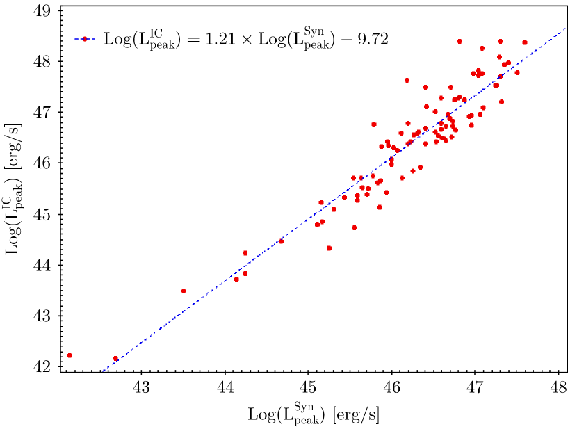
Figure 4: Syn vs. IC luminosity plane showing a tight correlation that extends for seven decades in luminosity. Blue dashed line is a linear fit to the data.

The correlation we see at the luminosity plane is probably related to a constant ratio between external photon field ($\rm U^{\prime}_{Ext}$) and the magnetic field ($\rm U^{\prime}_{B}$) energy densities in the jet comoving frame. Assuming an EC scenario in this case, this correlation could be taken as observational evidence of the established balance between a dynamic radiative-drag and the magnetic energy density. On the one hand, the radiative-drag is induced by the jet interaction with a boosted external photon field $U^{\prime}_{Ext}$, as discussed in Moderski et al. (2003) and Madejski et al. (1999), which is directly connected to the loss energy mechanism for the relativistic electrons (cooling) even imposing limitations to the jet’s Lorentz factor ($\Gamma$). On the other hand, following Keppens et al. (2008), the magnetic energy density $\rm U_{b}$ might be directly connected to the particles acceleration (energy gain – bulk plasma heating) and jet structure collimation.

Therefore, the argument put forward by Tavecchio et al. (1998) and Gao et al. (2011) where the ratio between IC and Syn luminosities are directly related to the energy densities $\rm U_{ext}$ and $\rm U_{b}$ is based on the underling dynamic-mechanisms at work, i.e., the mechanisms responsible for particle acceleration and deceleration within the jet structure. In fact, given that synchrotron and external photons might undergo IC scattering, $\rm L_{IC}\propto U^{\prime}_{Ext}+U^{\prime}_{Syn}$ should be more suitable for describing luminosity ratios in general, and $\rm L_{IC}\propto U^{\prime}_{Ext}$ might hold as the best approach to describe EC scenarios where $\rm U^{\prime}_{Ext}$ is dominant with respect to $\rm U^{\prime}_{Syn}$ (using “$\prime$” to refer to jet rest-frame quantities):

$$\rm\frac{L_{IC}}{L_{Syn}}=\frac{U^{\prime}_{Ext}+U^{\prime}_{Syn}}{U^{\prime}_{B}}\ \ (a)\Rightarrow\ \frac{U^{\prime}_{Ext}}{U^{\prime}_{B}}\ \ (b)$$ (7)

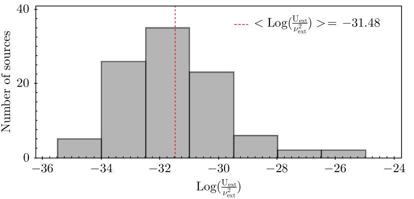
Figure 5: Distribution for the $\rm log(U_{ext}/\nu^{2}_{ext})$ parameter, as derived from eq. 8 when considering measurements from Table The $\gamma$-ray emitting region in low synchrotron peak blazars. The mean value associated with $\rm log(U_{ext}/\nu^{2}_{ext})$ is highlighted with dashed red line.

Also, we should note that the characteristic slope and tight correlation in the $\rm L_{IC}$ versus $\rm L_{Syn}$ plane is in agreement with the CD distribution for LSP blazars (as reported by Arsioli & Polenta, 2018), which is Gaussian-like and peaks at log(CD) slightly higher than zero, at $\rm\approx 0.17$. The fact that the slope associated with log(L_IC) versus log(L_Syn) is well established at $>$ 1.0 is probably related to the number of strong and fast flaring events in $\gamma$ rays which pushes the $\rm\langle L_{IC}\rangle$ to higher values when we integrate the observed flux from steady + flaring states over many years. In addition, it is telling us that the more powerful (luminous) blazars are the ones undergoing $\gamma$-ray flares more frequently. This could be a hint for the existence of an extra component apart from external and synchrotron photons that might be contributing to the IC bump during flaring events, especially for the most powerful (luminous) blazars. This is in agreement with the possibility of having hadronic or ultra-high-energy cosmic rays (UHECR) cascade components connected to the IC bump, just as considered by Cerruti et al. (2017a).

As discussed by Hu et al. (2017), contributions from external photon fields (IR and UV, from accretion disk, BLR, and dust Torus) are relevant for describing the HE bump from blazar SEDs, and currently the major difficulty is the lack of precise knowledge about the AGN environment so that a multicomponent EC model can be fitted properly. In this scenario, it is hard to conclude the most relevant $\gamma$-ray emission site for individual sources, but as we describe here (from our population studies) the IR field tends to be more suitable to model the IC component of bright LSP blazars. Therefore, on average, a far-site emission for MeV-GeV photons is favored, suggesting that an efficient acceleration mechanism might operate far from the core region, as mention by Sikora et al. (2009).

From Tavecchio et al. (1998) and Gao et al. (2011), when using eq. 7.b, the external photon density U_ext transforms to the jet comoving frame according to $\rm U^{\prime}_{ext}=(17/12)\Gamma^{2}U_{ext}$ as derived in Ghisellini & Madau (1996). Then, assuming the synchrotron peak $\rm\nu^{Syn}_{peak}=(4/3)\nu_{L}\gamma^{2}_{peak}\delta$ and $\rm\nu^{EC}_{peak}=(4/3)\nu^{ext}_{peak}\gamma^{2}_{peak}\Gamma\delta$, where $\rm\gamma_{peak}$ is the Lorentz factor for electrons emitting in the Syn peak, $\rm\nu_{L}=eB/(2\pi m_{e}c)$ is the Larmor frequency, and $\rm\nu^{ext}_{peak}$ is the peak frequency associated with the external photon field. From this Gao et al. (2011) obtain

$$\rm\frac{L_{IC}}{L_{Syn}}\simeq\frac{17e^{2}}{6\pi m_{e}^{2}c^{2}}\frac{U_{Ext}}{\nu^{2}_{ext}}\Big{(}\frac{\nu^{EC}_{peak}}{\nu^{S}_{peak}}\Big{)}^{2}$$ (8)

Using measured values for $\rm L_{Syn}$, $\rm L_{IC}$, and assuming $\rm\nu^{EC}_{peak}\equiv\nu^{IC}_{peak}$, with $\rm\frac{17e^{2}}{6\pi m_{e}^{2}c^{2}}=2.79\times 10^{14}$ [$\rm\frac{cm^{3}}{erg.s^{2}}$], we infer the distribution of energy density $\rm(U_{ext}/\nu^{2}_{ext})$ associated with the external photon field at the AGN source frame (fig. 5, which has mean value $\rm\langle log(U_{ext}/\nu^{2}_{ext})\rangle=-32.53\pm 0.17$ . Given the discussion from Sect. 4.2, if we assume the external photon field to be dominant in IR, with $\rm\nu_{ext}=\nu_{IR}=3\times 10^{13}$ Hz, the characteristic IR-photon energy density for LSP blazar under EC regime is $\rm\langle U_{ext}\rangle=2.98\times 10^{-5}$ erg/cm³ at the AGN rest frame; The photon field seen by the jet (comoving jet frame) is then: $\rm U^{\prime}_{ext}=(17/12)\Gamma^{2}U_{ext}=1.69\times 10^{-2}$ erg/cm³. Our estimate for $\rm\langle U^{\prime}_{ext}\rangle$ is in good agreement with Breiding et al. (2018), which assumes a far-site emission zone for $\gamma$-ray photons as a result of an IC upscattering of IR seed photons (originating from an illuminated molecular torus and assuming a spine-sheath geometry). We note that we follow the discussion from Sect. 4.2 and assume $\langle\Gamma\rangle=20$, the bulk Lorentz factor associated with the relativistic outflow.

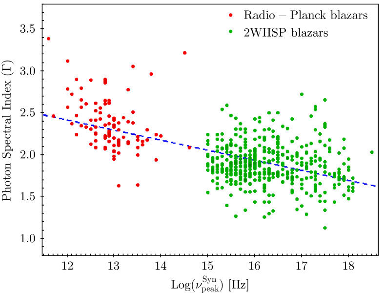
Figure 6: Gamma-ray photon spectral index ($\Gamma$) vs. the Syn peak $\rm log(\nu_{peak}^{Syn}$) parameter: in red, the radio-Planck sources (LSP blazars); in green, the 2WHSP sources (HSP blazars); blue dashed line is the linear fitting considering all sources in the $\Gamma$ vs. $\rm log(\nu_{peak}^{Syn}$) plane.

4.4 The $\gamma$-ray photon spectral index versus the synchrotron peak frequency

In Fig. 6 we show the correlation between the $\gamma$-ray photon spectral index and the logarithm of the Syn peak frequency log($\nu_{peak}^{Syn}$), considering all the 99 radio-Planck sources that had available data in the MeV to GeV band. To expand the description beyond LSP sources and extend the test to higher $\nu^{sync}_{peak}$ values, in this same plot we add the 2WHSP sources (Chang et al., 2017) which is a highly confident sample of high synchrotron peak (HSP) blazars. A linear fitting in the $\Gamma$ versus log($\nu_{peak}^{Syn}$) plane reveals a clear negative trend,

$$\rm\langle\Gamma\rangle=-0.119\times log(\langle\nu_{peak}^{Syn}\rangle)+3.85,$$ (9)

showing, on average, that increasing synchrotron peak frequency is related to the hardening of the $\gamma$-ray spectrum in the 0.1 to 500 GeV band, as also reported by Acero et al. (2015) and Arsioli et al. (2015). This is usually explained as a consequence of the fixed observational energy window from Fermi-LAT ($\sim$100 MeV up to 500 GeV) which probes different regions of the IC bump: after its peak (soft spectra with decaying power $\rm P_{(\nu)}$) in case of LSPs, and before its peak (hard spectra with increasing power $\rm P_{(\nu)}$) in the case of HSPs. This is usually taken as observational evidence that $\nu^{IC}_{peak}$ is moving to higher energies according to $\nu^{Syn}_{peak}$.

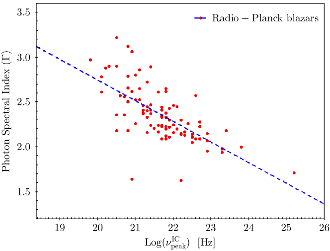
Figure 7: Gamma-ray photon spectral index ($\Gamma$) vs. the inverse Compton peak $\rm log(\nu_{peak}^{IC}$) parameter. In red, the radio-Planck sources with good estimates for the IC peak; the blue dashed line is the linear fitting for the data.

The connection between $\nu^{IC}_{peak}$ and $\nu^{Syn}_{peak}$ is actually very hard to probe directly, simply because we have limited data to describe the IC bump in the case of HSP blazars. For HSPs, the IC bump extends farther than the Fermi-LAT main sensitivity window, and despite the many detections with ground-based very high-energy observatories (VHE, at E $>$ 100 GeV), the absorption of VHE photons due to scattering with low-energy extragalactic background light (EBL) hinders the description of the IC peak.

If we consider only the complete radio-Planck sample of LSP blazars (Arsioli & Polenta, 2018), a scatter plot with $\rm log(\nu^{Syn}_{peak})$ versus $\rm log(\nu^{IC}_{peak})$ shows no clear correlation. A complete sample of blazars spanning a wider range in $\rm log(\nu_{peak})$ space might be needed to better probe the $\rm\nu^{Syn}_{peak}$ to $\rm\nu^{IC}_{peak}$ connection. In Fig. 7 we plot the $\gamma$-ray photon spectral index against the $\rm log(\nu_{peak}^{IC}$), this time only for the radio-Planck sources with good estimates for the IC parameter (cases with the ? flag in Table The $\gamma$-ray emitting region in low synchrotron peak blazars were eliminated). Even if we try to use a complete sample of HSP blazars, there is no good estimate of $\nu^{IC}_{peak}$ for all sources, and therefore we do not consider HSPs for this plot. A linear fitting in the $\Gamma$ versus $\rm log(\nu_{peak}^{IC}$) gives

$$\rm\langle\Gamma\rangle=-0.229\times log(\langle\nu_{peak}^{IC}\rangle)+7.34$$ (10)

Both correlations, as in eq. 9 and eq. 10, tell us that LSP blazars are associated with the steepest $\gamma$-ray sources in the 0.1–500 GeV band, with an IC peak located around the MeV band. Faint point-like sources of this kind are difficult to detect with Fermi-LAT, especially in regions close to the galactic disk $|b|<10^{\circ}$ where the MeV diffuse component is dominant. In pure leptonic SSC and EC scenarios, a correlation between spectral parameters derived from the Syn and IC components is expected (Giommi et al., 2012b, 2013) given that both components depend directly on the jet’s relativistic electrons producing synchrotron radiation and acting for the up-scattering of low-energy photons to $\gamma$ rays.

5 Conclusions

We evaluate the jet’s Lorentz factor $\gamma_{peak}$ and B$\delta$ parameters for LSP blazars in the radio-Planck sample, assuming at first a simple single-zone SSC model. In this case, we show that B$\delta$ is probably underestimated owing to overestimated $\gamma^{SSC}_{peak}$ values; therefore, a SSC model can hardly describe the SED observed for LSP blazars.

We studied the Tramacere plane $\rm log(\gamma^{SSC}_{peak})$ versus $\rm log(\nu^{Syn}_{peak})$ to show that most sources in the radio-Planck sample are above the limits associated with a dominant SSC regime. In fact, they populate a region that is characteristic of the EC regime under TH scattering, spreading along a parameter-space that is attributed to external photon fields ranging from IR to UV.

Assuming an EC model, we reevaluate the $\gamma^{EC}_{peak}$ and B$\delta$ parameters for LSP blazars. We assume two different external photon fields, one dominated by UV photons (consistent with BLR emission) and another dominated by IR photons (consistent with dust torus emission, and MC emission in spine-sheath geometry). We conclude that on average an IR field is probably more suitable, resulting in distributions with the corresponding mean values $\rm\langle log(B\delta)\rangle\approx 0.99$ and $\rm\langle log(\gamma^{EC}_{peak})\rangle\approx 2.80$ consistent with expectations from Kang et al. (2014) and Cao & Wang (2013). This hints to a $\gamma$-ray emission region which is out of the BLR domain, far from the BH, at a distance $\gg$ 0.1 pc. Moreover, it demands the jet structure to be a very narrow opening (or with substructures) to reconcile with the short timescale variability observed in the GeV-TeV band (Agudo et al., 2011). We calculate the photon energy density associated with the external field at the jet comoving frame to be $\rm U^{\prime}_{ext}=1.69\times 10^{-2}$ erg/cm³, finding good agreement with Breiding et al. (2018).

We calculate the luminosity associated with the peak-power for both Syn and IC components, and plot $\rm log(L_{IC})$ versus $\rm log(L_{Syn})$ in what we called “the luminosity plane”. There we show a tight correlation spanning seven orders of magnitude in luminosity, with slope slightly larger than one, which is probably related to a nearly constant ratio of the energy density associated with external + synchrotron photon fields to the magnetic energy density, ($\rm U^{\prime}_{Ext}+U^{\prime}_{Syn})/U^{\prime}_{B}$, implying a balance between the particle’s acceleration and deceleration mechanisms in the jet. In fact, the slope we measure in the luminosity plane is larger than 1.0 and could be induced by the $\gamma$-ray flaring activity, which is proving to be more relevant for the most luminous (powerful and extreme) sources.

We probe the correlation between the $\gamma$-ray photon spectral index (0.1–500 GeV band) with both $\rm\nu^{Syn}_{peak}$ and $\rm\nu^{IC}_{peak}$ parameters, showing a trend of hardening $\Gamma$ for increasing $\nu^{Syn}_{peak}$ and $\rm\nu^{IC}_{peak}$, noting that LSP blazars are characterized by steep $\gamma$-ray spectrum in the 0.1–500 GeV band, which hinders the detection of faint LSP sources with Fermi-LAT.

[x]¿p2.8cm¿p1.0cm—¿p1.0cm¿p1.0cm¿p1.0cm¿p1.0cm¿p1.0cm¿p1.0cm¿ p1.0cm¿ p1.0cm¿ p1.0cm Here we lits all 104 sources used for our studies. Column 5BZcat shows the blazar name according to Massaro et al. (2015) where BZQ stands for Flat Spectrum Radio Quasars, BZB for BL Lacs and BZU for still undefined-class blazars. Column z corresponds to the redshift as reported in the 5BZcat Massaro et al. (2015), and from the NASA-IPAC Extragalactic Database (NED). We list the fitting parameters characterizing the peak power for the synchrotron component log($\rm\nu_{Syn}$) [Hz]; log($\rm\nu$f${}^{Syn}_{\nu}$) [erg/cm²/s] and inverse Compton component log($\rm\nu_{IC}$) [Hz]; log($\rm\nu$f${}^{IC}_{\nu}$) [erg/cm²/s] as measured from the mean SED when considering all available data (Arsioli & Polenta 2018). The parameter log($\rm\gamma^{SSC}_{peak}$) corresponds to the Lorentz factor associated to relativistic electrons at the synchrotron peak-frequency when considering a pure SSC model (* in many cases leading to overestimate values). The parameter log($\rm\gamma^{EC}_{IR/UV}$) corresponds to the Lorentz factor when assuming an EC scenario with dominant IR seed photons from the dust and MC torus (denoted with IR suffix), and UV seed photons from accretion disk and BLR region (denoted with UV suffix). The log(B$\rm\delta_{IR}$) and log(B$\rm\delta_{UV}$) columns list the corresponding values for B$\rm\delta$ when assuming a dominant IR and UV external photon fields, respectively, with B given in Gauss and $\rm\delta$ representing the beaming factor. We would like to note that Arsioli & Polenta (2018) also list R.A., Dec. (J2000) and radio counterparts for each source according to NVSS catalog (Condon et al. 1998).
log log log log log log log log log
5BZcat J z $\nu_{Syn}$ $\nu$f${}^{Syn}_{\nu}$ $\nu_{IC}$ $\nu$f${}^{IC}_{\nu}$ $\gamma^{SSC}_{peak}$ $\gamma^{EC}_{IR}$ B$\delta_{IR}$$\gamma^{EC}_{UV}$ B$\delta_{UV}$
continued.
log log log log log log log log log
5BZcat J z $\nu_{Syn}$ $\nu$f${}^{Syn}_{\nu}$ $\nu_{IC}$ $\nu$f${}^{IC}_{\nu}$ $\gamma^{SSC}_{peak}$ $\gamma^{EC}_{IR}$ B$\delta_{IR}$$\gamma^{EC}_{UV}$ B$\delta_{UV}$
5BZBJ0050$-$0929 $...$ 14.6 $-$11.0 22.7 $-$11.1 3.98 3.24 1.59 2.33 2.51
5BZBJ0238+1636 0.94 13.0 $-$10.9 22.5 $-$10.4 4.68 3.29 0.19 2.37 1.11
5BZBJ0449+1121 2.153 12.9 $-$11.5 21.8 $-$10.8 4.38 3.04 0.79 2.13 1.71
5BZBJ0721+7120 $...$ 13.9 $-$10.3 23.3 $-$10.5 4.63 3.54 0.29 2.63 1.21
5BZBJ0738+1742 0.424 13.5 $-$10.6 23.8 $-$11.0 5.08 3.87 $-$0.60 2.96 0.31
5BZBJ0757+0956 0.266 13.7 $-$10.8 20.8 $-$11.1 3.48 2.34 2.59 1.43 3.51
5BZBJ0825+0309 0.506 13.1 $-$11.1 21.5(?) $-$11.6 4.13 2.73 1.29 1.82 2.21
5BZBJ0854+2006 0.306 13.6 $-$10.4 21.8 $-$10.8 4.03 2.85 1.49 1.94 2.41
5BZBJ0958+6533 0.367 13.4 $-$11.0 21.2 $-$11.3 3.83 2.56 1.89 1.65 2.81
5BZBJ1419+5423 0.153 13.7 -10.6 21.9 $-$11.5 4.03 2.87 1.49 1.96 2.41
5BZBJ1653+3945 0.033 17.8 $-$10.2 25.2 $-$10.6 3.63 4.50 2.29 3.59 3.21
5BZBJ1800+7828 0.68 13.5 $-$10.7 21.9 $-$10.9 4.13 2.96 1.29 2.04 2.21
5BZBJ1806+6949 0.046 14.0 $-$10.6 21.7 $-$11.0 3.78 2.75 1.99 1.84 2.91
5BZBJ1824+5651 0.663 13.2 $-$11.3 22.1 $-$11.0 4.38 3.05 0.79 2.14 1.71
5BZBJ2005+7752 0.342 13.2 $-$11.2 21.5 $-$11.3 4.08 2.71 1.39 1.79 2.31
5BZBJ2134$-$0153 1.283 12.8 $-$11.3 21.8 $-$11.5 4.43 2.97 0.69 2.06 1.61
5BZBJ2202+4216 0.069 13.6 $-$10.0 21.3 $-$10.3 3.78 2.56 1.99 1.65 2.91
5BZQJ0006$-$0623 0.347 13.0 $-$11.1 20.3 $-$11.9 3.58 2.11 2.39 1.20 3.31
5BZQJ0010+1058 0.089 14.5 $-$10.7 20.5 $-$10.8 2.93 2.16 3.69 1.25 4.61
5BZQJ0108+0135 2.099 12.9 $-$11.2 22.4 $-$10.6 4.68 3.34 0.19 2.43 1.11
5BZQJ0125$-$0005 1.077 12.8 $-$11.6 20.3 $-$11.6 3.68 2.20 2.19 1.29 3.11
5BZQJ0136+4751 0.859 13.3 $-$10.9 22.2 $-$10.7 4.38 3.13 0.79 2.22 1.71
5BZQJ0152+2207 1.32 12.9 $-$11.5 21.8 $-$11.5 4.38 2.98 0.79 2.06 1.71
5BZQJ0217+7349 2.367 12.2 $-$11.6 20.5 $-$10.4 4.08 2.41 1.39 1.49 2.31
5BZQJ0228+6721 0.523 12.8 $-$11.2 21.1 $-$11.4 4.08 2.53 1.39 1.62 2.31
5BZQJ0237+2848 1.206 12.9 $-$11.2 22.0 $-$10.7 4.48 3.06 0.59 2.15 1.51
5BZQJ0309+1029 0.863 12.8 $-$11.2 21.7 $-$11.2 4.38 2.88 0.79 1.97 1.71
5BZQJ0336+3218 1.259 12.8 $-$11.3 20.2 $-$10.5 3.63 2.17 2.29 1.26 3.21
5BZQJ0339$-$0146 0.805 12.6 $-$11.3 22.0 $-$11.1 4.63 3.02 0.29 2.11 1.21
5BZQJ0359+5057 1.512 12.1 $-$10.7 21.3 $-$10.4 4.53 2.74 0.49 1.83 1.41
5BZQJ0423$-$0120 0.916 13.0 $-$10.6 22.1 $-$10.7 4.48 3.08 0.59 2.17 1.51
5BZQJ0501$-$0159 2.291 13.0 $-$11.4 21.4 $-$11.1 4.13 2.85 1.29 1.94 2.21
5BZQJ0510+1800 0.416 13.3 $-$11.3 21.3 $-$11.1 3.93 2.62 1.69 1.71 2.61
5BZQJ0530+1331 2.07 12.2 $-$11.5 21.4 $-$10.7 4.53 2.84 0.49 1.92 1.41
5BZQJ0555+3948 2.365 12.0 $-$11.7 20.8 $-$10.9 4.33 2.56 0.89 1.64 1.81
5BZQJ0607$-$0834 0.87 12.1 $-$11.5 21.4 $-$11.0 4.58 2.73 0.39 1.82 1.31
5BZQJ0646+4451 3.396 11.6 $-$11.8 21.8(?) $-$11.5 5.03 3.11 $-$0.50 2.20 0.41
5BZQJ0739+0137 0.189 13.9 $-$10.9 21.6 $-$10.8 3.78 2.73 1.99 1.82 2.91
5BZQJ0750+1231 0.889 12.6 $-$11.1 21.2 $-$11.2 4.23 2.63 1.09 1.72 2.01
5BZQJ0808+4950 1.432 12.0 $-$12.2 20.6 $-$11.7 4.23 2.39 1.09 1.47 2.01
5BZQJ0808$-$0751 1.837 13.0 $-$11.1 22.9 $-$10.7 4.88 3.57 $-$0.20 2.66 0.71
5BZQJ0830+2410 0.939 12.6 $-$11.1 21.8 $-$11.0 4.53 2.94 0.49 2.02 1.41
5BZQJ0841+7053 2.218 12.4 $-$11.3 20.1 $-$10.2 3.78 2.20 1.99 1.28 2.91
5BZQJ0920+4441 2.19 12.5 $-$11.2 22.3 $-$10.6 4.83 3.29 $-$0.10 2.38 0.81
5BZQJ0927+3902 0.695 12.1 $-$11.2 $...$ $...$ $-$6.1 $-$7.9 21.7 $-$8.89 22.7
5BZQJ0948+4039 1.249 12.3 $-$11.8 20.8 $-$11.2 4.18 2.47 1.19 1.56 2.11
5BZQJ0956+2515 0.712 12.7 $-$11.4 21.9 $-$11.4 4.53 2.96 0.49 2.05 1.41
5BZQJ1038+0512 0.473 12.0 $-$11.8 20.8 $-$12.1 4.33 2.38 0.89 1.47 1.81
5BZQJ1043+2408 0.56 12.9 $-$11.5 21.7 $-$11.6 4.33 2.84 0.89 1.93 1.81
5BZQJ1130+3815 1.733 12.3 $-$11.7 22.6 $-$11.6 5.08 3.41 -0.60 2.50 0.31
5BZQJ1153+4931 0.334 12.9 $-$10.9 21.2 $-$11.1 4.08 2.56 1.39 1.64 2.31
5BZQJ1153+8058 1.25 12.6 $-$12.0 21.1 $-$11.9 4.18 2.62 1.19 1.71 2.11
5BZQJ1159+2914 0.729 13.5 $-$11.1 22.6 $-$10.8 4.48 3.31 0.59 2.40 1.51
5BZQJ1222+0413 0.966 12.7 $-$11.2 20.8 $-$10.7 3.98 2.44 1.59 1.53 2.51
5BZQJ1224+2122 0.434 13.1 $-$10.7 23.0 $-$10.0 4.88 3.47 $-$0.20 2.56 0.71
5BZQJ1229+0203 0.158 13.4 $-$10.0 20.8 $-$9.54 3.63 2.32 2.29 1.41 3.21
5BZQJ1256$-$0547 0.536 12.8 $-$10.0 22.7 $-$10.0 4.88 3.34 $-$0.20 2.42 0.71
5BZQJ1327+2210 1.398 12.6 $-$11.7 21.7 $-$11.0 4.48 2.93 0.59 2.02 1.51
5BZQJ1504+1029 1.839 12.8 $-$11.6 22.9 $-$10.0 4.98 3.57 $-$0.40 2.66 0.51
5BZQJ1512$-$0905 0.36 13.1 $-$10.9 22.2 $-$9.91 4.48 3.06 0.59 2.15 1.51
5BZQJ1549+0237 0.414 12.9 $-$11.2 22.0 $-$11.1 4.48 2.97 0.59 2.06 1.51
5BZQJ1550+0527 1.422 13.0 $-$11.4 21.8 $-$11.4 4.33 2.99 0.89 2.07 1.81
5BZQJ1608+1029 1.226 12.8 $-$11.3 21.6 $-$11.0 4.33 2.87 0.89 1.95 1.81
5BZQJ1613+3412 1.397 12.3 $-$11.5 21.7 $-$11.6 4.63 2.93 0.29 2.02 1.21
5BZQJ1635+3808 1.814 12.5 $-$11.1 21.7 $-$10.3 4.53 2.97 0.49 2.06 1.41
5BZQJ1640+3946 1.66 12.9 $-$11.9 22.7 $-$10.8 4.83 3.46 $-$0.10 2.54 0.81
5BZQJ1642+3948 0.593 13.0 $-$10.6 21.7 $-$10.7 4.28 2.84 0.99 1.93 1.91
5BZQJ1642+6856 0.751 12.5 $-$11.6 20.1(?) $-$12.3 3.73 2.06 2.09 1.15 3.01
5BZQJ1740+5211 1.381 13.2 $-$11.3 21.3 $-$10.8 3.98 2.73 1.59 1.82 2.51
5BZQJ1743$-$0350 1.057 12.6 $-$11.3 21.0 $-$11.2 4.13 2.55 1.29 1.64 2.21
5BZQJ1849+6705 0.657 13.1 $-$10.9 22.5 $-$10.6 4.63 3.25 0.29 2.34 1.21
5BZQJ1927+7358 0.302 13.1 $-$10.8 $...$ $...$ $-$6.6 $-$8.0 22.7 $-$8.95 23.7
5BZQJ1955+5131 1.214 12.7 $-$11.7 20.7 $-$11.4 3.93 2.42 1.69 1.50 2.61
5BZQJ2007+4029 1.736 12.2 $-$11.6 $...$ $...$ $-$6.1 $-$7.8 21.8 $-$8.79 22.8
5BZQJ2022+6136 0.228 12.9 $-$11.2 $...$ $...$ $-$6.5 $-$8.0 22.5 $-$8.96 23.5
5BZQJ2038+5119 1.686 12.5 $-$11.5 21.4 $-$11.0 4.38 2.81 0.79 1.90 1.71
5BZQJ2123+0535 1.941 12.6 $-$11.7 21.6 $-$11.8 4.43 2.93 0.69 2.02 1.61
5BZQJ2136+0041 1.941 11.7 $-$11.6 21.2 $-$11.2 4.68 2.73 0.19 1.82 1.11
5BZQJ2139+1423 2.427 12.2 $-$11.7 $...$ $...$ $-$6.1 $-$7.85 21.8 $-$8.74 22.8
5BZQJ2148+0657 0.999 12.5 $-$10.8 20.5 $-$11.0 3.93 2.29 1.69 1.38 2.61
5BZQJ2203+1725 1.076 13.3 $-$10.9 22.9 $-$10.9 4.73 3.50 0.09 2.59 1.01
5BZQJ2203+3145 0.295 13.4 $-$10.9 20.9 $-$11.1 3.68 2.40 2.19 1.49 3.11
5BZQJ2218$-$0335 0.901 12.3 $-$11.3 21.0 $-$11.7 4.28 2.53 0.99 1.62 1.91
5BZQJ2225$-$0457 1.404 13.0 $-$10.8 21.7 $-$10.9 4.28 2.93 0.99 2.02 1.91
5BZQJ2229$-$0832 1.56 13.1 $-$11.2 21.8 $-$10.5 4.28 3.00 0.99 2.09 1.91
5BZQJ2232+1143 1.037 12.4 $-$11.2 21.3 $-$10.5 4.38 2.70 0.79 1.79 1.71
5BZQJ2236+2826 0.79 13.0 $-$11.2 22.5 $-$10.9 4.68 3.27 0.19 2.36 1.11
5BZQJ2253+1608 0.859 13.1 $-$10.0 22.2 $-$9.2 4.48 3.13 0.59 2.22 1.51
5BZQJ2354+4553 1.992 12.2 $-$11.9 21.4 $-$11.7 4.53 2.83 0.49 1.92 1.41
5BZQJ2356+8152 1.344 12.8 $-$11.8 21.1 $-$11.5 4.08 2.63 1.39 1.72 2.31
5BZUJ0102+5824 0.644 12.6 $-$11.1 21.8 $-$10.9 4.53 2.90 0.49 1.99 1.41
5BZUJ0204+1514 0.833 12.6 $-$11.6 21.0 $-$11.2 4.13 2.52 1.29 1.61 2.21
5BZUJ0241$-$0815 0.005 13.5 $-$10.1 20.9(?) $-$10.6 3.63 2.34 2.29 1.43 3.21
5BZUJ0319+4130 0.018 13.0 $-$10.4 23.3 $-$10.4 5.08 3.55 $-$0.60 2.63 0.31
5BZUJ0433+0521 0.033 13.8 $-$10.2 19.8 $-$10.2 2.93 1.80 3.69 0.89 4.61
5BZUJ0725$-$0054 0.128 13.5 $-$11.0 20.5 $-$11.2 3.43 2.17 2.69 1.26 3.61
5BZUJ0909+4253 0.67 12.9 $-$11.5 20.9 $-$11.7 3.93 2.45 1.69 1.54 2.61
5BZUJ1058+0133 0.89 13.1 $-$10.9 22.3 $-$10.8 4.53 3.18 0.49 2.27 1.41
5BZUJ1310+3220 0.997 13.1 $-$10.8 22.2 $-$10.8 4.48 3.14 0.59 2.23 1.51
5BZUJ1415+1320 0.247 12.8 $-$11.0 20.5 $-$11.2 3.78 2.19 1.99 1.28 2.91
5BZUJ1751+0939 0.322 13.1 $-$10.8 21.9 $-$10.8 4.33 2.90 0.89 1.99 1.81
5BZUJ1829+4844 0.695 13.0 $-$11.3 20.7 $-$11.1 3.78 2.36 1.99 1.45 2.91
3C111 0.0485 13.3 $-$10.6 20.1 $-$10.0 3.33 1.95 2.89 1.04 3.81
M87 0.0042 13.0 $-$10.5 18.5(?) $-$10.4 2.68 1.14 4.19 0.23 5.11