On the calculation of the correlation functions of the $\mathfrak{sl}_{3}$-model by means of the reduced qKZ equation

Abstract.

We study the reduced density matrix of the $\mathfrak{sl}_{3}$-invariant fundamental exchange model by means of a novel reduced quantum Knizhnik-Zamolodchikov equation. This gives us insight into the algebraic structure and explicit results for correlation functions in the infinite chain ranging over up to three sites.

1. Introduction

Over the past three decades considerable progress has been made in the study of correlation functions of integrable models, in particular, of the integrable spin-1/2 Heisenberg-Ising (or XXZ) chain associated with the affine quantum group $U_{q}(\widehat{\mathfrak{sl}}_{2})$. Due to this progress we are nowadays able to compute the static correlation functions of this model under very general equilibrium conditions at short and large distances and with arbitrary numerical accuracy [1, 2, 3, 4, 5, 6]. What may be considered even more important is that we may have uncovered part of the mathematical structure that seems to distinguish the correlation functions of integrable systems from those of non-integrable ones. As far as the mathematical structure and the short-range correlation functions are concerned it turned out to be particularly fruitful to study the reduced density matrix of a finite connected chain segment of the XXZ chain and its inhomogeneous multi-spectral-parameter version associated with the underlying six-vertex model. Starting with the pioneering work [7] of the ‘Kyoto school’ a number of rather diverse methods have been applied in order to derive various representations of the reduced density matrix as well as general theorems about its structure. In [7] a multiple-integral representation for the ground-state correlation functions of the XXZ chain in the massive regime was obtained by means of a ‘q-vertex operator approach’ based on the representation theory of $U_{q}(\widehat{\mathfrak{sl}}_{2})$ and inspired by Baxter’s corner transfer matrix method [8] and by conformal field theory [9]. A generalization to the massless regime was obtained in [10] using a different method based on functional equations in the spectral parameters of qKZ-type [11, 12]. These results were further generalized, utilizing the Bethe Ansatz, to include a longitudinal magnetic field [13] and arbitrary finite temperatures [14].

In papers [15], it was observed that the multiple integrals representing the ground-state correlation functions at vanishing magnetic field factorize in products of one-dimensional integrals, this way reproducing a singular and puzzling result of Takahashi [16] from the 70s. In collaboration of one of the authors with M. Jimbo, T. Miwa, F. Smirnov and Y. Takeyama the algebraic structure behind the factorization of the multiple integrals was eventually unveiled [17, 18]. Creation and annihilation operators on a space of quasi-local operators were constructed in such a way that the creation operators generate a special ‘fermionic basis’ by iterated action on an appropriate Fock vacuum [18, 19]. Jimbo, Miwa and Smirnov [20] then proved an important theorem showing that, under very general conditions, the correlation functions corresponding to any quasi-local operator can be related to only two functions $\rho$ and $\omega$ through a determinant formula. The function $\rho$ is a spectral-parameter dependent one-point function, basically equal to the magnetization, while $\omega$ is a two-point function depending on two spectral parameters. It can be interpreted as an expectation value of a special operator of length 2 or a special nearest-neighbour two-point correlation function. In this sense $\omega$ is very similar to the energy density. Thus, the theorem of Jimbo, Miwa and Smirnov states that the two most local non-trivial, independent correlation functions determine all others through algebraic relations. Moreover all physical parameters, like system length, temperature or magnetic field enter only through these two functions which turn out to have efficient descriptions in terms of solutions of linear and non-linear integral equations [21].

It would appear natural if a similar structure, implying that all static correlation functions are algebraically determined by a few short-range correlation functions, would exist for other, more complicated integrable systems as well. Arguably, next in complexity, after the basic models related to $U_{q}(\widehat{\mathfrak{sl}}_{2})$, come their higher-rank generalizations or the rational counterparts of these models. Extending and elaborating the works [22, 23], two of the authors studied the functional equations related to their spectrum by means of representation theory and gave their full proof in a universal form in joint work with Göhmann, Klümper and Razumov [24].

Studies of the spectral problem of these higher rank models, especially in their rational, $\mathfrak{sl}(N)$-symmetric version have a long history starting with the pioneering works by Yang [25] and Sutherland [26] on the multi-component Bose and Fermi gases. In paper [27], Sutherland considered the diagonalization problem of the Hamiltonian

$$H=\pm\sum\limits_{j=1}^{L}P_{j,j+1}$$ (1.1)

with periodic boundary conditions, where the operator $P$ permutes local states of $N$ Bosons and $M$ Fermions. Nowadays we would call this Hamiltonain the $\mathfrak{sl}(N|M)$-invariant exchange Hamiltonian. Sutherland was the first to diagonalize it by nested Bethe Ansatz. A nested algebraic Bethe ansatz was later developed by Kulish and Reshetikhin [28, 29]. The $R$-matrix which is relevant in the $\mathfrak{sl}(N)$-case is proportional to the $S$-matrix of the $SU(N)$ Gross-Neveu model, which is an interesting quantum field theory associated with a higher rank quantum group [30, 31, 32, 33].

The correlation functions of relativistic quantum field theories can be studied starting from solutions to a set of functional equations known as the ‘form factor axioms’ [34, 35]. The form factors give access to correlation functions through certain spectral representations alias sums over multiple integrals which are often useful for asymptotic analysis. Form factors for lattice models like (1.1) are less constrained. They have not been obtained as solutions of functional equations, but in recent years have been constructed by algebraic Bethe ansatz methods [36, 37]. It seems however difficult to sum them up to correlation functions, especially at short-distances. The only more concrete result for correlation functions that has been obtained so far by means of the lattice form-factor approach concerns the two-point functions at large distances [38].

In papers [40, 39] the vertex-operator approach was used to obtain the multiple integral representation for the $U_{q}(\hat{\mathfrak{sl}}_{n})$ model in critical and massive regimes. Unfortunately, the formulas are rather bulky and are given only up to the normalization. This certainly makes a precise numerical computation difficult.

It is moreover unclear if an algebraic structure, similar to the one identified for the XXZ model, exists for the fundamental $\mathfrak{sl}_{3}$ lattice model.

In this paper we consider the rational $\mathfrak{sl}_{3}$-model with Hamiltonian (1.1) at zero temperature and zero external fields. Since we were unable to directly generalize the hidden fermionic structure of the $\mathfrak{sl}_{2}$-case we shall follow the original idea that led to its discovery. We shall derive a reduced quantum Knizhnik-Zamolodchikov equation (rqKZ) introduced for the $\mathfrak{sl}_{2}$-case in [41]. Then we solve the novel rqKZ equation for $n=1,2,3$ lattice sites, giving us direct analytical results for the reduced density matrices of chain segments of the respective length. Note that the rqKZ equation was not known for the $\mathfrak{sl}_{3}$-case and that, as we shall see, a generalization from $\mathfrak{sl}_{2}$ to $\mathfrak{sl}_{3}$ is not as straightforward as it might appear, since there is no crossing symmetry in the higher-rank case. Our results for the short-range correlation functions for $n=2,3$ are, to the best of our knowledge, the first explict results for correlation functions of this model. The case $n=4$ is considerably more complicated. We will describe it in a separate publication. The purpose and the driving force behind our work is the hope to identify a minimal number of independent short-range correlation functions that will determine all correlation functions of the model at larger distances.

The plan of the paper is as follows. In Section 2, we describe the integrable structure of the $\mathfrak{sl}_{3}$-model. We introduce the corresponding $R$-matrix and recall some of its properties, such as unitarity and crossing relations. In Section 3, we discuss static correlation functions, related density matrices, inhomogeneous generalizations and their basic properties. Section 4 is the main section of this work. Here we introduce a pair of reduced qKZ equations and the resulting closed rqKZ equation for the generalized density matrix which we solve for three lengths of the corresponding local operators, $n=1,2,3$. To solve this equation, we introduce two transcendental functions $\omega^{(1)}$ and $\omega^{(3)}$ and discuss their properties. We also discuss the homogeneous limit of the formulas we have obtained for the density matrices. Section 5 is devoted to conclusions. In Appendix A, we provide a heuristic derivation of our rqKZ equation based on a technique developed by Aufgebauer and Klümper for the $\mathfrak{sl}_{2}$-case at finite temperature [42]. In Appendix B, we show some details of the derivation of the integral representation of our function $\omega^{(3)}$ in homogeneous case.

2. The rational $\mathfrak{sl}_{3}$ model

Let us start with the formulation of the model. In the more general case, including a deformation parameter $q$, the $R$-matrix is defined in the tensor product of two representation spaces of $U_{q}(\widehat{\mathfrak{sl}}_{3})$. The Khoroshkin–Tolstoy formula [43] for the universal $R$-matrix allows one to obtain the $R$-matrix for arbitrary representations in the so-called auxiliary and quantum spaces [44], but we are firstly interested in the case of two fundamental representations. Taking the limit $q\to 1$ in the expression for the $U_{q}(\widehat{\mathfrak{sl}}_{3})$-related $R$-matrix from [44], we reproduce the $R$-matrix of the rational $\mathfrak{sl}_{3}$-model under consideration. It has a particularly simple form

$$\displaystyle{R_{12}(\lambda)}=\frac{\rho(\lambda)}{\lambda+1}\bigl{(}\lambda\;\mathbf{1}_{12}+P_{12}\bigr{)},$$ (2.1)

where $\mathbf{1}_{12}$ and $P_{12}$ are the $3^{2}\times 3^{2}$ unit and permutation matrices, respectively, acting in the tensor product of spaces $1$ and $2$ in the case of three states or “colors”, and the function $\rho$ can be regarded as a quasi-classical, $q\to 1$, or the rational, limit of the transcendental pre-factor obtained from the Khoroshkin–Tolstoy formula. In our case, it satisfies two functional relations

$$\rho(\lambda)\rho(-\lambda)=1,\qquad\rho(\lambda)\rho(3-\lambda)=\frac{(\lambda-3)\;\lambda}{(\lambda-1)(\lambda-2)},$$ (2.2)

an appropriate solution of which can explicitly be written in the form

$$\displaystyle\rho(\lambda)=-\frac{\Gamma(\lambda/3)\Gamma(1/3-\lambda/3)}{\Gamma(-\lambda/3)\Gamma(1/3+\lambda/3)}.$$ (2.3)

Alternatively, $\rho(\lambda)$ can be obtained using the algebraic structure of the Yangian double of $\mathfrak{sl}_{3}(\mathbb{C})$ [12, 45].

Also we need to define matrices $\bar{R}$ and $\bar{\bar{R}}$ acting in the tensor product of fundamental and anti-fundamental representations and in the tensor product of anti-fundamental and fundamental representations, respectively. To this end, we use the corresponding crossing relations

$${\bar{R}}_{1\bar{2}}(\lambda)=C_{\bar{2},2}{\bigl{(}R_{12}(-\lambda-1)\bigr{)}}^{t_{2}}C_{2,\bar{2}},$$

$${\bar{\bar{R}}}_{\bar{1}2}(\lambda)=C_{\bar{1},1}{\bigl{(}R_{12}(-\lambda-2)\bigr{)}}^{t_{1}}C_{1,\bar{1}},$$ (2.4)

where $t_{j}$ denotes the transposition in space $j$ and $C_{\bar{j},j}=C_{j,\bar{j}}$ stand for the “charge conjugation” matrix $C$

$$C=\begin{pmatrix}0&0&1\\ 0&1&0\\ 1&0&0\end{pmatrix}.$$ (2.5)

Below we will use $C_{i,\bar{j}}=C_{\bar{j},i}$ for incoming lines $i$ and $\bar{j}$ and $C^{i,\bar{j}}=C^{\bar{j},i}$ for the outgoing lines $i$ and $\bar{j}$. In both cases it is again given by (2.5).

When it does not cause any misunderstanding, we will just write $R_{i,j}$ for $R_{i,j}(\lambda_{i,j})$, where $\lambda_{i,j}=\lambda_{i}-\lambda_{j}$ and similarly for the other $R$-matrices $\bar{R}$ and $\bar{\bar{R}}$. We can also explicitly write down

$${\bar{R}}(\lambda)=\frac{\bar{\rho}(\lambda)}{\lambda}\bigl{(}\lambda+1-C\otimes C\bigr{)},\quad{\bar{\rho}}(\lambda)={\rho}(\lambda+1)^{-1},$$ (2.6)

$${\bar{\bar{R}}}(\lambda)={\bar{R}}(\lambda+1).$$

An important immediate consequence of this formula and definition (2.1) is that

$$R(0)=P,\quad{\bar{R}}(-1)={\bar{\bar{R}}}(-2)=C\otimes C.$$ (2.7)

For later usage we will also need four relations which are consequences of the Yang–Baxter equation and the above crossing relations (2.4) and (2.7):

$$R_{1,3}(\lambda_{1,3})\,{\bar{\bar{R}}}_{\bar{2},3}(\lambda_{1,3}-2)\,C_{1,\bar{2}}=\mathbf{1}_{3}\;C_{1,\bar{2}},\quad{\bar{R}}_{1,\bar{3}}(\lambda_{1,3})\,R_{\bar{2},\bar{3}}(\lambda_{1,3}-2)\,C_{1,\bar{2}}=\mathbf{1}_{\bar{3}}\;C_{1,\bar{2}},$$ (2.8)

$${\bar{\bar{R}}}_{\bar{1},3}(\lambda_{1,3})\,R_{2,3}(\lambda_{1,3}-1)\,C_{\bar{1},2}=\mathbf{1}_{3}\;C_{\bar{1},2},\quad R_{\bar{1},\bar{3}}(\lambda_{1,3})\,{\bar{R}}_{2,\bar{3}}(\lambda_{1,3}-1)\,C_{\bar{1},2}=\mathbf{1}_{\bar{3}}\;C_{\bar{1},2}.$$ (2.9)

It is not difficult to verify these relations directly.

3. Static correlation functions and density matrix

If one takes all external fields to be zero, the quasi-local operators become just local operators. In this case the static zero temperature correlation function of some local operator $X_{1,\ldots,n}$ defined on a lattice segment of the length $n$ is the vacuum expectation value

$$\langle\text{vac}|X_{1,\ldots,n}|\text{vac}\rangle=D\bigl{(}X_{1,\ldots,n}\bigr{)},$$ (3.1)

where $|\text{vac}\rangle$ corresponds to the ground state of the model in the thermodynamic limit. $D$ stands for the density matrix acting on a local operator $X$. As was discussed in papers [18, 20], it is a functional which maps any operator $X_{1,\ldots,n}$ to a number. The elements of the density matrix are defined as follows:

$$D_{i_{1},\cdots,i_{n}}^{i^{\prime}_{1},\ldots,i^{\prime}_{n}}=D(E_{i_{1}}^{i^{\prime}_{1}}\otimes\cdots\otimes E_{i_{n}}^{i^{\prime}_{n}}),$$ (3.2)

where $E_{i}^{i^{\prime}}$ are the elements of the basis of $\mathrm{Mat}_{3}(\mathbb{C})$ corresponding to the standard basis of $\mathbb{C}^{3}$, and so, these are the standard matrix units. We will also use the shorthand notation $D_{1,\ldots,n}$.

A useful trick is to introduce the inhomogeneity parameters $\lambda_{1},\ldots,\lambda_{n}$ for the above segment of length $n$. The new ground state will depend on these parameters

$$|\text{vac}\rangle\to|\text{vac}_{\{\lambda_{1},\ldots,\lambda_{n}\}}\rangle.$$

One can define a generalized density matrix which also depends on $\lambda_{1},\ldots,\lambda_{n}$:

$$\langle\text{vac}_{\{\lambda_{1},\ldots,\lambda_{n}\}}|X_{1,\ldots,n}|\text{vac}_{\{\lambda_{1},\ldots,\lambda_{n}\}}\rangle=D(\lambda_{1},\ldots,\lambda_{n})\bigl{(}X_{1,\ldots,n}\bigr{)},$$ (3.3)

with the corresponding matrix elements $D_{1,\ldots,n}(\lambda_{1},\ldots,\lambda_{n})$ defined in the same way as in (3.2). The generalized density matrix shows much more structure. We will see that this information can help us to find an explicit solution for the generalized density matrix. After such a solution is found, one can obtain the original density matrix by taking the homogeneous limit

$$D_{1,\ldots,n}=\lim_{\lambda_{1}\rightarrow 0,\ldots,\lambda_{n}\rightarrow 0}D_{1,\ldots,n}(\lambda_{1},\ldots,\lambda_{n}).$$ (3.4)

Let us list some important properties of the generalized density matrix.

1. The normalization condition

   $$D(\lambda_{1},\ldots,\lambda_{n})(\mathbf{1}_{1,\ldots,n})=1$$ (3.5)

   is consistent with the reduction relations.

2. Left–right reduction relations

   $$D(\lambda_{1},\ldots,\lambda_{n})(\mathbf{1}_{1}X_{2,\ldots,n})=D(\lambda_{2},\ldots,\lambda_{n})(X_{2,\ldots,n}),$$

   $$D(\lambda_{1},\ldots,\lambda_{n})(X_{1,\ldots,n-1}\mathbf{1}_{n})=D(\lambda_{1},\ldots,\lambda_{n-1})(X_{1,\ldots,n-1}).$$ (3.6)

3. The asymptotic condition

   $$\lim_{\lambda_{1}\to\infty}D_{1,\ldots,n}(\lambda_{1},\ldots,\lambda_{n})=\frac{1}{3}\;\mathbf{1}_{1}\;D_{2,\ldots,n}(\lambda_{2},\ldots,\lambda_{n}).$$ (3.7)

4. The $R$-matrix relations

   $$D_{1,\ldots,i,i+1,\ldots,n}(\lambda_{1},\ldots,\lambda_{n})\bigl{(}R_{i,i+1}(\lambda_{i,i+1})X_{1,\ldots,n}R_{i+1,i}(\lambda_{i+1,i})\bigr{)}$$

   $$=D_{1,\ldots,i+1,i,\ldots,n}(\lambda_{1},\ldots,\lambda_{i+1},\lambda_{i},\ldots\lambda_{n})\bigl{(}X_{1,\ldots,n}\bigr{)}.$$ (3.8)

5. The translational invariance

   $$D(\lambda_{1}+u,\ldots,\lambda_{n}+u)=D(\lambda_{1},\ldots,\lambda_{n})$$ (3.9)

   implying that the generalized density matrix elements depend only on differences $\lambda_{i}-\lambda_{j}$.

6. The global ${GL}_{3}$-invariance

   $$G\otimes\cdots\otimes G\;\Bigl{(}D(\lambda_{1},\ldots,\lambda_{n})\Bigr{)}\;G^{-1}\otimes\cdots\otimes G^{-1}=D(\lambda_{1},\ldots,\lambda_{n}),$$ (3.10)

   where $G$ is any element of the ${GL}_{3}(\mathbb{C})$ group in the fundamental representation.

7. The color conservation

   $$D(\lambda_{1},\ldots,\lambda_{n})_{i_{1},\ldots,i_{n}}^{i^{\prime}_{1},\ldots,i^{\prime}_{n}}\neq 0,\quad\text{only if}\quad n_{1}(\{i\})=n_{1}(\{i^{\prime}\}),$$

   $$\quad n_{2}(\{i\})=n_{2}(\{i^{\prime}\}),\quad n_{3}(\{i\})=n_{3}(\{i^{\prime}\}),$$ (3.11)

   where $n_{j}(\{i\})$ is the number of indices of “color” $j$ in the $n$-tuple $\{i\}=\{i_{1},\ldots,i_{n}\}$. There is a symmetry with respect to permutations of colors.

The above properties (i)–(v) are rather similar to the corresponding properties in the $\mathfrak{sl}_{2}$-case. Therefore, we will not prove them here. The properties (vi), (vii) follow directly from the characteristics of the $R$-matrix (2.1).

4. The rqKZ equations for the rational $\mathfrak{sl}_{3}$ model

Our experience with the $\mathfrak{sl}_{2}$-case suggests that the above properties do not fix the correlation functions uniquely. The missing information is hidden in a set of additional equations of difference type which were called the reduced qKZ equation [41]. We need to deduce such equations for the $\mathfrak{sl}_{3}$-case as well. This is done heuristically in Appendix A, where we obtain the following pair of difference equations:

$$D(\lambda_{1},\lambda_{2},\ldots,\lambda_{n})\Bigl{(}A^{(1)}_{1,\bar{1}|2,\ldots,n}(\lambda_{1}|\lambda_{2},\ldots,\lambda_{n})\bigl{(}X_{1,2,\ldots,n}\bigr{)}\Bigr{)}=D^{(1)}(\lambda_{1}-2,\lambda_{2},\ldots,\lambda_{n})\bigl{(}X_{\bar{1},2,\ldots,n}\bigr{)},$$ (4.1)

$$D^{(1)}(\lambda_{1},\lambda_{2},\ldots,\lambda_{n})\Bigl{(}A^{(2)}_{\bar{1},1|2,\ldots,n}(\lambda_{1}|\lambda_{2},\ldots,\lambda_{n})\bigl{(}X_{\bar{1},2,\ldots,n}\bigr{)}\Bigr{)}=\ D(\lambda_{1}-1,\lambda_{2},\ldots,\lambda_{n})\bigl{(}X_{1,2,\ldots,n}\bigr{)}.$$ (4.2)

Here the density matrix $D^{(1)}$ describes the situation with one anti-fundamental representation in the first quantum space and fundamental representations associated with the other spaces $2\cdots n$ (as depicted in Fig. 4 of Appendix A in the more general case). The operator $A^{(1)}_{1,\bar{1}|2,\cdots,n}$ is defined as follows: it acts on some local operator $X_{\bar{1},2,\cdots,n}$ as a matrix ${\Bigl{(}{A^{(1)}}_{a}^{b}\Bigr{)}}_{\bar{1}|2,\cdots,n}$ with respect to the space 1 with incoming line $a$ and outgoing line $b$

$${\bigl{(}{A^{(1)}}_{a}^{b}\bigr{)}}_{\bar{1}|2,\ldots,n}(\lambda_{1}|\lambda_{2},\ldots,\lambda_{n})\bigl{(}X_{\bar{1},2,\ldots,n}\bigr{)}\\ :=C^{\bar{1},b}R_{2,b}(\lambda_{2,1})\cdots R_{n,b}(\lambda_{n,1})X_{\bar{1},2,\ldots,n}R_{b,n}(\lambda_{1,n})\cdots R_{b,2}(\lambda_{1,2})C_{\bar{1},a},$$ (4.3)

and the operator $A^{(2)}_{\bar{1},1|2,\ldots,n}$ acts on some local operator $X_{1,\ldots,n}$ as a matrix with respect to the space $\bar{1}$ with incoming line $\bar{a}$ and outgoing line $\bar{b}$

$${\bigl{(}{A^{(2)}}_{\bar{a}}^{\bar{b}}\bigr{)}}_{1|2,\ldots,n}(\lambda_{1}|\lambda_{2},\ldots,\lambda_{n})\bigl{(}X_{1,2,\ldots,n}\bigr{)}\\ :=C^{1,\bar{b}}{\bar{R}}_{2,\bar{b}}(\lambda_{2,1})\cdots{\bar{R}}_{n,\bar{b}}(\lambda_{n,1})X_{1,2,\ldots,n}{\bar{\bar{R}}}_{\bar{b},n}(\lambda_{1,n})\cdots{\bar{\bar{R}}}_{\bar{b},n}(\lambda_{1,2})C_{1,\bar{a}}.$$ (4.4)

In Appendix A we also show the above equations graphically in Fig. 7 and Fig. 8.

Combining equations (4.1) and (4.2), we come to a novel closed reduced qKZ equation (rqKZ) which will be the key relation for solving the problem of the calculation of correlation functions in case of the $\mathfrak{sl}_{3}$-invariant model:

$$D(\lambda_{1},\ldots,\lambda_{n})\Bigl{(}A_{1|2,\ldots,n}(\lambda_{1}|\lambda_{2},\ldots,\lambda_{n})\bigl{(}X_{1,2,\ldots,n}\bigr{)}\Bigr{)}=D(\lambda_{1}-3,\ldots,\lambda_{n})\bigl{(}X_{1,2,\ldots,n}\bigr{)}.$$ (4.5)

Here

$$A(\lambda_{1}|\lambda_{2},\ldots,\lambda_{n})=A^{(1)}(\lambda_{1}|\lambda_{2},\ldots,\lambda_{n})A^{(2)}(\lambda_{1}-2|\lambda_{2},\ldots,\lambda_{n})$$ (4.6)

by definition. Since this formula looks a bit formal, let us explicitly write down the action of this operator on some local operator $X$. It acts with respect to the first space as a matrix ${(A_{a}^{b})}_{2,\ldots,n}(\lambda_{1}|\lambda_{2},\ldots,\lambda_{n})$ with incoming line $a$ and outgoing line $b$:

$${(A_{a}^{b})}_{2,\ldots,n}(\lambda_{1}|\lambda_{2},\ldots,\lambda_{n})(X_{1,\ldots,n})\\ =C^{\bar{1},b}R_{2,b}(\lambda_{2,1})\cdots R_{n,b}(\lambda_{n,1})C^{1,\bar{a}}{\bar{R}}_{2,\bar{a}}(\lambda_{2,1}+2)\cdots{\bar{R}}_{n,\bar{a}}(\lambda_{n,1}+2)\bigl{(}X_{1,\ldots,n}\bigr{)}\\ \times{\bar{\bar{R}}}_{\bar{a},n}(\lambda_{1,n}-2)\cdots{\bar{\bar{R}}}_{\bar{a},2}(\lambda_{1,2}-2)R_{b,n}(\lambda_{1,n})\cdots R_{b,2}(\lambda_{1,2})C_{\bar{a},a}C_{1,\bar{1}}.$$ (4.7)

The corresponding picture is given in Appendix A (see Fig. 9).

So far, we have been able to solve the whole set of relations (3.6)–(3.10) together with the rqKZ equation (4.5) up to the length $n=3$. We present our results below.

4.1. The case $n=1$.

From the above symmetry and normalization (3.5) we immediately come to the conclusion that

$${D(\lambda_{1})}_{i}^{j}=\frac{1}{3}\delta_{i}^{j}.$$ (4.8)

The rqKZ relation (4.5) gives in this case the following simple equation:

$${D(\lambda_{1})}_{i}^{j}={D(\lambda_{1}-3)}_{i}^{j},$$ (4.9)

which is compatible with solution (4.8). One can easily check that all other relations (3.6)–(3.10) are fulfilled automatically.

4.2. The case $n=2$.

The case $n=2$ is more substantial. From the color conservation property (3.11) we conclude that there are only three non-trivial non-zero elements

$$D_{0}(\lambda_{1},\lambda_{2})={D(\lambda_{1},\lambda_{2})}_{i,i}^{i,i}\quad\text{for}\quad i=1,2,3,$$ (4.10)

$$D_{1}(\lambda_{1},\lambda_{2})={D(\lambda_{1},\lambda_{2})}_{i,j}^{i,j},\quad D_{2}(\lambda_{1},\lambda_{2})={D(\lambda_{1},\lambda_{2})}_{i,j}^{j,i}\quad\text{for}\quad i,j=1,2,3\quad\text{and}\quad i\neq j.$$

From the global $GL_{3}$-invariance (3.10) it follows that the density matrix is of the form

$$D_{1,2}(\lambda_{1},\lambda_{2})=\mathbf{1}_{1,2}\,D_{1}(\lambda_{1},\lambda_{2})+P_{1,2}\,D_{2}(\lambda_{1},\lambda_{2}).$$ (4.11)

Certainly, the subscripts 1 and 2 of the functions $D_{1},D_{2}$ in this formula should not be mixed up with the numbers of spaces 1 and 2.

Thus, we can immediately obtain the functions $D_{0}$ and $D_{1}$ from the reduction relations (3.6). We have

$$D_{0}(\lambda_{1},\lambda_{2})=D_{1}(\lambda_{1},\lambda_{2})+D_{2}(\lambda_{1},\lambda_{2})=\frac{1}{3}-2D_{1}(\lambda_{1},\lambda_{2}),$$ (4.12)

and so,

$$D_{1}(\lambda_{1},\lambda_{2})=\frac{1}{9}-\frac{1}{3}D_{2}(\lambda_{1},\lambda_{2}).$$ (4.13)

From the $R$-matrix invariance (3.8) and translational invariance (3.9) it follows that the function $D_{2}$ is symmetric

$$D_{2}(\lambda_{1},\lambda_{2})=D_{2}(\lambda_{2},\lambda_{1}),\quad$$ (4.14)

and depends on the difference of the spectral parameters. Let us choose it in the following form:

$$D_{2}(\lambda_{1},\lambda_{2})=-3\,\omega^{(1)}(\lambda_{1,2}),$$ (4.15)

where $\omega^{(1)}(\lambda)$ is an even function of $\lambda$. With this choice formula (4.11) becomes

$$D_{1,2}(\lambda_{1},\lambda_{2})=\frac{1}{9}\mathbf{1}_{1,2}+\omega^{(1)}(\lambda_{1,2})\,P^{(0)}_{1,2},$$ (4.16)

where the notation

$$P^{(0)}_{1,2}=\mathbf{1}_{1,2}-3P_{1,2}$$ (4.17)

is introduced.

Now we have to solve the rqKZ relation. To this end, we can substitute formula (4.16) into the rqKZ relation (4.5) and note that

$$P^{(0)}_{1,2}A_{1|2}(\lambda_{1}|\lambda_{2})=P^{(1)}(\lambda_{1,2})P^{(0)}_{1,2},$$ (4.18)

$$\mathbf{1}_{1,2}A_{1|2}(\lambda_{1}|\lambda_{2})=\mathbf{1}_{1,2}+9\,Q^{(1)}(\lambda_{1,2})P^{(0)}_{1,2},$$ (4.19)

where $P^{(1)},Q^{(1)}$ are rational functions

$$P^{(1)}(\lambda)=\frac{(\lambda-4)(\lambda-2)}{(\lambda-1)(\lambda+1)},\quad Q^{(1)}(\lambda)=-\frac{2\lambda-3}{3(\lambda-3)(\lambda-1)\lambda(\lambda+1)}.$$ (4.20)

We see that the operator $P^{(0)}$ turns out to be a constant eigenvector of the operator $A$ with the eigenvalue $P^{(1)}(\lambda)$. Two relations (4.18), (4.19) are in fact nothing but the reduction of the rqKZ equation to the triangular form. Therefore, if we act on $A$ by the right-hand side of (4.16), use formula (4.18), (4.19) and equate the coefficients standing before the identity operator and the operator $P^{(0)}$, we come to the following functional relation for the function $\omega^{(1)}$:

$$\omega^{(1)}(\lambda-3)=P^{(1)}(\lambda)\omega^{(1)}(\lambda)+Q^{(1)}(\lambda).$$ (4.21)

This equation is nothing but the result of diagonalization of the rqKZ equation, which is related to a certain non-local matrix Riemann–Hilbert problem. It is not clear yet how to find its solution in general case.

It is interesting to note that the coefficients $P^{(1)}$ and $Q^{(1)}$ should satisfy certain compatibility condition

$$P^{(1)}(3-\lambda)P^{(1)}(\lambda)=1,\quad P^{(1)}(3-\lambda)Q^{(1)}(\lambda)+Q^{(1)}(3-\lambda)=0,$$ (4.22)

which might be seen as a zero curvature condition in some geometric picture. We will consider this question in more detail elsewhere.

The solution to the above functional relation (4.21) looks as

$$\omega^{(1)}(\lambda)=-\frac{1}{36}+\frac{\lambda^{2}-1}{24}\bar{\omega}^{(1)}(\lambda),$$ (4.23)

where the function

$$\bar{\omega}^{(1)}(\lambda)=-\frac{\partial}{\partial\lambda}\log{\rho(\lambda)}$$ (4.24)

satisfies the functional equation

$$\bar{\omega}^{(1)}(\lambda-3)=\bar{\omega}^{(1)}(\lambda)+\bar{Q}^{(1)}(\lambda)$$ (4.25)

with

$$\bar{Q}^{(1)}(\lambda)=\frac{1}{\lambda-3}-\frac{1}{\lambda-2}-\frac{1}{\lambda-1}+\frac{1}{\lambda}=\frac{2(2\lambda-3)}{(\lambda-3)(\lambda-2)(\lambda-1)\lambda}.$$ (4.26)

For later use we will need two further representations of the function $\bar{\omega}^{(1)}(\lambda)$:

$$\bar{\omega}^{(1)}(\lambda)\!\!\! = \!\!\!-\frac{1}{3}\Bigl{(}\psi\Bigl{(}\frac{\lambda}{3}\Bigr{)}+\psi\Bigl{(}-\frac{\lambda}{3}\Bigr{)}-\psi\Bigl{(}\frac{1}{3}+\frac{\lambda}{3}\Bigr{)}-\psi\Bigl{(}\frac{1}{3}-\frac{\lambda}{3}\Bigr{)}\Bigr{)}$$ (4.27)

$$= \!\!\!-\sum_{j=0}^{\infty}\Bigl{(}\frac{1}{\lambda-3j}-\frac{1}{\lambda+3j}+\frac{1}{\lambda+1+3j}-\frac{1}{\lambda-1-3j}\Bigr{)},$$ (4.28)

where $\psi(\lambda)$ is the logarithmic derivative of the $\Gamma$-function. Bellow we will also use $\psi_{n}(\lambda)=\partial_{\lambda}^{n}\psi(\lambda)$.

Thus, we obtain the entries of the generalized density matrix

$${D(\lambda_{1},\lambda_{2})}_{i,i}^{i,i}=D_{0}(\lambda_{1},\lambda_{2})=\frac{1}{9}-2\,\omega^{(1)}(\lambda_{1,2}),$$

$${D(\lambda_{1},\lambda_{2})}_{i,j}^{i,j}=D_{1}(\lambda_{1},\lambda_{2})=\frac{1}{9}+\omega^{(1)}(\lambda_{1,2}),$$ (4.29)

$${D(\lambda_{1},\lambda_{2})}_{i,j}^{j,i}=D_{2}(\lambda_{1},\lambda_{2})=-3\,\omega^{(1)}(\lambda_{1,2}),$$

where it is implied that $i\neq j$ in last two equations.

Since for large values of $|\lambda|$ we have

$$\bar{\omega}^{(1)}(\lambda)\simeq\frac{2}{3}\lambda^{-2}-\frac{2}{3}\lambda^{-4}+\mathcal{O}(\lambda^{-6}),$$

the asymptotic behavior of the function $\omega^{(1)}(\lambda)$ is as follows:

$$\omega^{(1)}(\lambda)\simeq-\frac{1}{18}\,\lambda^{-2}+\mathcal{O}(\lambda^{-4})\quad{\mbox{ when}}\quad{|\lambda|\to\infty}.$$ (4.30)

Using this formula, we can easily check the asymptotic relation (3.7). It means that our result (4.29) fulfills the rqKZ relation (4.5) and all the above properties (i)–(vii).

Now it is easy to obtain the elements of the original density matrix taking the homogeneous limit (3.4), since the value of the function $\omega^{(1)}(\lambda)$ at $\lambda=0$ is well defined

$$\displaystyle\omega^{(1)}(0)=\lim_{\lambda\to 0}\omega^{(1)}(\lambda)=-\frac{1}{36}\Bigl{(}1+\gamma+\psi\bigl{(}\frac{1}{3}\bigr{)}\Bigr{)},$$ (4.31)

where $\gamma$ is Euler’s constant.

Finally, the result for the density matrix in the $n=2$ case looks as follows:

$${\displaystyle D_{i,i}^{i,i}=\frac{1}{9}-2\omega^{(1)}(0)=\frac{1}{6}+\frac{1}{18}\Bigl{(}\gamma+\psi\bigl{(}\frac{1}{3}\bigr{)}\Bigr{)}=\frac{1}{6}-\frac{\pi}{36\sqrt{3}}-\frac{\log{3}}{12}=0.0247323...}$$

$${\displaystyle D_{i,j}^{i,j}=\frac{1}{9}+\omega^{(1)}(0)=\frac{1}{12}-\frac{1}{36}\Bigl{(}\gamma+\psi\bigl{(}\frac{1}{3}\bigr{)}\Bigr{)}=\frac{1}{12}+\frac{\pi}{72\sqrt{3}}+\frac{\log{3}}{24}=0.154301...}$$ (4.32)

$${\displaystyle D_{i,j}^{j,i}=-3\,\omega^{(1)}(0)=\frac{1}{12}\Bigl{(}1+\gamma+\psi\bigl{(}\frac{1}{3}\bigr{)}\Bigr{)}=\frac{1}{12}-\frac{\pi}{24\sqrt{3}}-\frac{\log{3}}{8}=-0.129568...}$$

where we imply that $i,j=1,2,3$ and $i\neq j$.

Let us compare this with our numerical result obtained by direct diagonalization of the transfer matrix up to the lengths $L=9,12$ (see Table 1)

	$D_{1,2}^{1,2}$	$D_{2,1}^{1,2}$
Exact result ($L=\infty$)	0.1543	-0.129568
L=9	0.15546	-0.133048
L=12	0.154946	-0.131505

Table 1. Comparison of numerical and analytic results for $D_{2}$

4.3. The case $n=3$.

In a sense, the above result for the density matrix for $n=2$ is rather similar to the $\mathfrak{sl}_{2}$-case, where the function $\omega$ there was related to the logarithmic derivative of the pre-factor of the $R$-matrix [41]. We will see that the situation with the $n=3$ case is essentially different since it will be necessary to involve one more function of three spectral parameters. Technically, the case $n=3$ is more intricate, and some formulas become rather tedious. Therefore, let us only roughly describe our basic steps that we made in order to come to the final result.

1. The first step is to use the global $GL_{3}$-invariance (3.10) in order to write the elements of the generalized density matrix in the following form:

   $${D(\lambda_{1},\lambda_{2},\lambda_{3})}_{i_{1},i_{2},i_{3}}^{i^{\prime}_{1},i^{\prime}_{2},i^{\prime}_{3}}=\sum_{\sigma\in\mathcal{S}_{3}}g^{(\sigma)}(\lambda_{1},\lambda_{2},\lambda_{3})\;\delta_{i_{1}}^{i^{\prime}_{\sigma(1)}}\delta_{i_{2}}^{i^{\prime}_{\sigma(2)}}\delta_{i_{3}}^{i^{\prime}_{\sigma(3)}},$$ (4.33)

   where the sum goes over all six elements $\sigma$ of the permutation group $\mathcal{S}_{3}$ with six unknown functions $g^{(\sigma)}(\lambda_{1},\lambda_{2},\lambda_{3})$.

2. The second step is to fulfill the $R$-matrix relations (3.8) together with the reduction relations (3.6). At this stage we need to solve some functional relations in order to express the above six unknown functions $g^{(\sigma)}(\lambda_{1},\lambda_{2},\lambda_{3})$ in terms of five fully symmetric functions $\tilde{g}^{(i)}(\lambda_{1},\lambda_{2},\lambda_{3})$ with $i=1,\cdots,5$.

3. The third step is to solve the rqKZ equation (4.5) with respect to these five functions. At this stage we observe that the final answer is a sum of three terms: the first one is proportional to the identity operator which reduces by relations (3.6) to the identity operator in the $n=2$ case in (4.29), the second term reduces to terms containing the function $\omega^{(1)}$, and the third term has zero reduction both from the left and from the right. This third term is proportional to a new fully symmetric function $\omega^{(3)}(\lambda_{1},\lambda_{2},\lambda_{3})$. With the help of the rqKZ equation (4.5) we find that the function $\omega^{(3)}$ should fulfill certain functional relation which we discuss below.

Let us show the result:

$$D_{1,2,3}(\lambda_{1},\lambda_{2},\lambda_{3})=\frac{1}{27}\mathbf{1}_{1,2,3}\\ +f_{1,2,3}^{(12)}(\lambda_{1},\lambda_{2}|\lambda_{3})\;\omega^{(1)}(\lambda_{1,2})+f_{1,2,3}^{(13)}(\lambda_{1},\lambda_{2},\lambda_{3})\;\omega^{(1)}(\lambda_{1,3})+f_{1,2,3}^{(23)}(\lambda_{1}|\lambda_{2},\lambda_{3})\;\omega^{(1)}(\lambda_{2,3})\\ +f_{1,2,3}^{(123)}\;\omega^{(3)}(\lambda_{1},\lambda_{2},\lambda_{3}),$$ (4.34)

where $f^{(ij)}$ are matrices with rational elements

$$f_{1,2,3}^{(12)}(\lambda_{1},\lambda_{2}|\lambda_{3})=R_{1,2}\;f_{2,1,3}^{(12)}(\lambda_{2},\lambda_{1}|\lambda_{3})\;R_{1,2}^{-1}\\ =\Bigl{(}1-\frac{1}{\lambda_{1,3}\lambda_{2,3}}\Bigr{)}\Bigl{(}\frac{1}{3}-P_{1,2}\Bigr{)}+\frac{1}{\lambda_{1,3}\lambda_{2,3}}P_{2,3}+\frac{1}{2}\Bigl{(}\frac{\lambda_{1,2}-3}{\lambda_{1,3}\lambda_{2,3}}P_{2,3}P_{1,2}-\frac{\lambda_{1,2}+3}{\lambda_{1,3}\lambda_{2,3}}P_{1,2}P_{2,3}\Bigr{)},$$ (4.35)

$$f_{1,2,3}^{(13)}(\lambda_{1},\lambda_{2},\lambda_{3})=R_{2,3}\;f_{1,3,2}^{(12)}(\lambda_{1},\lambda_{3}|\lambda_{2})\;R_{2,3}^{-1}\\ =\Bigl{(}1-\frac{1}{\lambda_{2,1}\lambda_{2,3}}\Bigr{)}\Bigl{(}\frac{1}{3}-P_{1,3}\Bigr{)}+\frac{1}{\lambda_{2,1}\lambda_{2,3}}(P_{1,2}+P_{2,3}-P_{1,3})\\ +\frac{1}{2}\Bigl{(}\frac{\lambda_{2,1}+\lambda_{2,3}-3}{\lambda_{2,1}\lambda_{2,3}}P_{1,2}P_{2,3}-\frac{\lambda_{2,1}+\lambda_{2,3}+3}{\lambda_{2,1}\lambda_{2,3}}P_{2,3}P_{1,2}\Bigr{)},$$ (4.36)

$$f_{1,2,3}^{(23)}(\lambda_{1}|\lambda_{2},\lambda_{3})=R_{2,3}\;f_{1,3,2}^{(23)}(\lambda_{1}|\lambda_{3},\lambda_{2})\;R_{2,3}^{-1}=R_{1,2}\;f_{2,1,3}^{(13)}(\lambda_{2},\lambda_{1},\lambda_{3})\;R_{1,2}^{-1}\\ =\Bigl{(}1-\frac{1}{\lambda_{1,2}\lambda_{1,3}}\Bigr{)}\Bigl{(}\frac{1}{3}-P_{2,3}\Bigr{)}+\frac{1}{\lambda_{1,2}\lambda_{1,3}}P_{1,2}+\frac{1}{2}\Bigl{(}\frac{\lambda_{2,3}-3}{\lambda_{1,2}\lambda_{1,3}}P_{1,2}P_{2,3}-\frac{\lambda_{2,3}+3}{\lambda_{1,2}\lambda_{1,3}}P_{2,3}P_{1,2}\Bigr{)}.$$ (4.37)

Here we did not write the identity operators in order not to overload the formulas.

The coefficient $f^{(123)}$ in the last term in (4.34) can be written in two ways

$$f^{(123)}_{1,2,3}=\frac{16}{9}\Bigl{(}1-\frac{3}{2}(P_{1,2}+P_{1,3})\Bigr{)}\Bigl{(}1-\frac{3}{2}P_{2,3}\Bigr{)}=\frac{16}{9}\Bigl{(}1-\frac{3}{2}P_{1,2}\Bigr{)}\Bigl{(}1-\frac{3}{2}(P_{1,3}+P_{2,3})\Bigr{)},$$ (4.38)

where the zero left reduction is evident from the first formula and the zero right reduction is evident from the second one. Also one can check that (4.38) satisfies the $R$-matrix relations

$$f_{1,2,3}^{(123)}=R_{1,2}\;f_{2,1,3}^{(123)}\;R_{1,2}^{-1}=R_{2,3}\;f_{1,3,2}^{(123)}\;R_{2,3}^{-1}.$$ (4.39)

Note that, as in the case $n=2$, the coefficient $f^{(123)}$ is the eigenvector of the $A$-operator which does not depend on the spectral parameters:

$$f^{(123)}_{1,2,3}A_{1|23}(\lambda_{1}|\lambda_{2},\lambda_{3})=P^{(3)}(\lambda_{1}|\lambda_{2},\lambda_{3})\;f^{(123)}_{1,2,3},$$ (4.40)

where the rational function $P^{(3)}(\lambda_{1}|\lambda_{2},\lambda_{3})$ is defined below.

As we announced above, the function $\omega^{(3)}(\lambda_{1},\lambda_{2},\lambda_{3})$ is symmetric with respect to its arguments and satisfies the functional relation

$$\omega^{(3)}(\lambda_{1}-3,\lambda_{2},\lambda_{3})=P^{(3)}(\lambda_{1}|\lambda_{2},\lambda_{3})\;\omega^{(3)}(\lambda_{1},\lambda_{2},\lambda_{3})\\ +P^{(3,1)}(\lambda_{1}|\lambda_{2}|\lambda_{3})\;\omega^{(1)}(\lambda_{12})+P^{(3,1)}(\lambda_{1}|\lambda_{3}|\lambda_{2})\;\omega^{(1)}(\lambda_{13})+P^{(3,2)}(\lambda_{1}|\lambda_{2},\lambda_{3})\;\omega^{(1)}(\lambda_{23})\\ +Q^{(3)}(\lambda_{1}|\lambda_{2},\lambda_{3})$$ (4.41)

with the rational functions

$$P^{(3)}(\lambda_{1}|\lambda_{2},\lambda_{3})=\frac{(\lambda_{1,2}-4)(\lambda_{1,2}-2)\lambda_{1,2}}{(\lambda_{1,2}-3)(\lambda_{1,2}-1)(\lambda_{1,2}+1)}\cdot\frac{(\lambda_{1,3}-4)(\lambda_{1,3}-2)\lambda_{1,3}}{(\lambda_{1,3}-3)(\lambda_{1,3}-1)(\lambda_{1,3}+1)},$$ (4.42)

$$P^{(3,1)}(\lambda_{1}|\lambda_{2}|\lambda_{3})=\frac{9(\lambda_{1,2}-4)(\lambda_{1,2}-2)\lambda_{1,2}}{8(\lambda_{1,2}-1)(\lambda_{1,2}+1)(\lambda_{1,3}-3)(\lambda_{1,3}-1)(\lambda_{1,3}+1)\lambda_{2,3}},$$ (4.43)

$$P^{(3,2)}(\lambda_{1}|\lambda_{2},\lambda_{3})=-\frac{9(\lambda_{1,2}+\lambda_{1,3}-3)(\lambda_{2,3}^{2}-9)}{8(\lambda_{1,2}-3)(\lambda_{1,2}-1)(\lambda_{1,2}+1)(\lambda_{1,3}-3)(\lambda_{1,3}-1)(\lambda_{1,3}+1)},$$ (4.44)

$$Q^{(3)}(\lambda_{1}|\lambda_{2},\lambda_{3})=-\frac{\lambda_{1,2}+\lambda_{1,3}-6}{8(\lambda_{1,2}-3)(\lambda_{1,2}-1)(\lambda_{1,2}+1)(\lambda_{1,3}-3)(\lambda_{1,3}-1)(\lambda_{1,3}+1)}.$$ (4.45)

As in the $n=2$ case, the functions $P^{(3)},P^{(3,1)},P^{(3,2)}$ and $Q^{(3)}$ must satisfy a set of compatibility conditions coming from the equation $\omega^{(3)}(\lambda_{1}-3,\lambda_{2}-3,\lambda_{3}-3)=\omega^{(3)}(\lambda_{1},\lambda_{2},\lambda_{3})$ and consequent application of the functional relation (4.41). Let us show only one of them:

$$P^{(3)}(\lambda_{1}|\lambda_{2}-3,\lambda_{3}-3)P^{(3)}(\lambda_{2}|\lambda_{1},\lambda_{3}-3)P^{(3)}(\lambda_{3}|\lambda_{1},\lambda_{2})=1.$$ (4.46)

In fact, we have thus reduced the non-local matrix RH-problem (3.5)–(3.11), (4.5) for $n=2,3$ to a non-local one-dimensional RH-problem.

Going backwards, it is not difficult to check that expression (4.34) satisfies the rqKZ equation (4.5). It also satisfies the $R$-matrix relation (3.8) and the left and right reduction relations (3.6).

Of course, the solution of the difference relation (4.41) is not unique. From the asymptotic condition (3.7) we can conclude that the function $\omega^{(3)}$ must decrease as some power of spectral parameters when they become large. It fixes the unique solution. Our analysis of the asymptotic behavior at large spectral parameters shows that

$$\omega^{(3)}(\lambda_{1},\lambda_{2},\lambda_{3})\simeq\lambda_{3}^{-4}\Bigl{(}-\frac{\lambda_{1,2}^{2}-9}{8}\;\omega^{(1)}(\lambda_{1,2})-\frac{1}{144}\Bigr{)}+\mathcal{O}(\lambda_{3}^{-5})\quad{\mbox{ when}}\quad\lambda_{3}\to\infty.$$ (4.47)

Now, the asymptotic condition (3.7) for $n=3$ can be checked using (4.30) and (4.47). This proves that expression (4.34) really satisfies the whole set of properties (i)–(vii) from Section 3 and the reduced qKZ relation (4.5).

4.4. Homogeneous limit

In order to obtain the elements of the original density matrix (3.2), we need to take the homogeneous limit $\lambda_{i}\to 0,i=1,2,3$ of the expression (4.34). To this end we should calculate

$$\omega^{(3)}(\vec{0}):=\lim_{\lambda_{1}\to 0,\lambda_{2}\to 0,\lambda_{3}\to 0}\omega^{(3)}(\lambda_{1},\lambda_{2},\lambda_{3}).$$ (4.48)

We do it in three steps.

First, we introduce the function

$$\bar{\omega}^{(3)}(\lambda_{1},\lambda_{2},\lambda_{3})=\prod_{j=2}^{3}\frac{\lambda_{1,j}}{(\lambda_{1,j}-1)(\lambda_{1,j}+1)}\omega^{(3)}(\lambda_{1},\lambda_{2},\lambda_{3}),$$ (4.49)

which satisfies the functional relation

$$\bar{\omega}^{(3)}(\lambda_{1}-3,\lambda_{2},\lambda_{3})=\bar{\omega}^{(3)}(\lambda_{1},\lambda_{2},\lambda_{3})\\ +\bar{P}^{(3,1)}(\lambda_{1}|\lambda_{2}|\lambda_{3})\bar{\omega}^{(1)}(\lambda_{1,2})+\bar{P}^{(3,1)}(\lambda_{1}|\lambda_{3}|\lambda_{2})\bar{\omega}^{(1)}(\lambda_{1,3})+\bar{P}^{(3,2)}(\lambda_{1}|\lambda_{2},\lambda_{3})\bar{\omega}^{(1)}(\lambda_{2,3})\\ +\bar{Q}^{(3)}(\lambda_{1}|\lambda_{2}|\lambda_{3}),$$ (4.50)

where the function $\bar{\omega}^{(1)}$ was defined in (4.24)–(4.28), and the functions $\bar{P}$ and $\bar{Q}$ explicitly are

$$\bar{P}^{(3,1)}(\lambda_{1}|\lambda_{2}|\lambda_{3})=\frac{3}{64}\cdot\frac{(\lambda_{1,2}-3)\lambda_{1,2}}{(\lambda_{1,3}-4)(\lambda_{1,3}-2)(\lambda^{2}_{1,3}-1)\lambda_{2,3}},$$ (4.51)

$$\bar{P}^{(3,2)}(\lambda_{1}|\lambda_{2},\lambda_{3})=-\frac{3}{64}\cdot\frac{(\lambda_{1,2}+\lambda_{1,3}-3)(\lambda_{2,3}^{2}-9)(\lambda_{2,3}^{2}-1)}{(\lambda_{1,2}-4)(\lambda_{1,2}-2)(\lambda^{2}_{1,2}-1)(\lambda_{1,3}-4)(\lambda_{1,3}-2)(\lambda^{2}_{1,3}-1)},$$ (4.52)

$$\bar{Q}^{(3)}(\lambda_{1}|\lambda_{2},\lambda_{3})=\frac{1}{32}\cdot\frac{(\lambda_{1,2}+\lambda_{1,3})(\lambda_{1,2}^{2}+\lambda_{1,3}^{2}+\lambda_{2,3}^{2}+13)-3(\lambda_{1,2}\lambda_{1,3}+4\lambda_{1,2}^{2}+4\lambda_{1,3}^{2})+27}{(\lambda_{1,2}-4)(\lambda_{1,2}-2)(\lambda^{2}_{1,2}-1)(\lambda_{1,3}-4)(\lambda_{1,3}-2)(\lambda^{2}_{1,3}-1)}.$$ (4.53)

From definition (4.49) and the asymptotic behavior (4.47) we deduce that

$$\bar{\omega}^{(3)}(\lambda_{1},\lambda_{2},\lambda_{3})\simeq\mathcal{O}(\lambda_{1}^{-6})\quad{\mbox{at}}\quad\lambda_{1}\to\infty.$$ (4.54)

Our second step is to take the limit with respect to $\lambda_{2},\lambda_{3}$:

$$\bar{\bar{\omega}}^{(3)}(\lambda):=\bar{\omega}^{(3)}(\lambda,0,0).$$ (4.55)

From the functional relation (4.50) and definitions (4.51)–(4.53) we deduce that the function $\bar{\bar{\omega}}^{(3)}$ must satisfy the following relation:

$$\bar{\bar{\omega}}^{(3)}(\lambda-3)-\bar{\bar{\omega}}^{(3)}(\lambda)=r(\lambda),$$ (4.56)

where

$$r(\lambda)=p^{(3,1)}_{1}(\lambda)\bar{\omega}^{(1)}(\lambda)+p^{(3,1)}_{2}(\lambda)\partial_{\lambda}\bar{\omega}^{(1)}(\lambda)+p^{(3,2)}(\lambda)\bar{\omega}^{(1)}(0)+q^{(3)}(\lambda)$$ (4.57)

and

$$p^{(3,1)}_{1}(\lambda)=-\frac{3}{64}\cdot\frac{(2\lambda-3)(3\lambda^{4}-18\lambda^{3}+23\lambda^{2}+12\lambda-8)}{(\lambda-4)^{2}(\lambda-2)^{2}(\lambda-1)^{2}(\lambda+1)^{2}},$$ (4.58)

$$p^{(3,1)}_{2}(\lambda)=-\frac{3}{64}\cdot\frac{(\lambda-3)\lambda}{(\lambda-4)(\lambda-2)(\lambda-1)(\lambda+1)},$$ (4.59)

$$p^{(3,2)}(\lambda)=-\frac{27}{64}\cdot\frac{2\lambda-3}{(\lambda-4)^{2}(\lambda-2)^{2}(\lambda-1)^{2}(\lambda+1)^{2}},$$ (4.60)

$$q^{(3)}(\lambda)=\frac{1}{32}\cdot\frac{4\lambda^{3}-27\lambda^{2}+26\lambda+27}{(\lambda-4)^{2}(\lambda-2)^{2}(\lambda-1)^{2}(\lambda+1)^{2}},$$ (4.61)

and from (4.54) it follows that

$$\bar{\bar{\omega}}^{(3)}(\lambda)\simeq\mathcal{O}(\lambda^{-6})\quad{\mbox{at}}\quad\lambda\to\infty.$$ (4.62)

Using the functional relation (4.25), one can make sure that

$$r(3-\lambda)=-r(\lambda).$$ (4.63)

Hence, if we transform $\lambda\to 3-\lambda$ in (4.56) and add both equations, we come to the relation

$$\bar{\bar{\omega}}^{(3)}(\lambda)-\bar{\bar{\omega}}^{(3)}(-\lambda)=\bar{\bar{\omega}}^{(3)}(\lambda-3)-\bar{\bar{\omega}}^{(3)}(3-\lambda),$$ (4.64)

which means that $\bar{\bar{\omega}}^{(3)}(\lambda)-\bar{\bar{\omega}}^{(3)}(-\lambda)$ must be a periodic function of $\lambda$ with the period $3$. But from the asymptotic behavior (4.62) we see that this function is $0$. We thus come to the conclusion that the function $\bar{\bar{\omega}}^{(3)}(\lambda)$ must be even

$$\bar{\bar{\omega}}^{(3)}(\lambda)=\bar{\bar{\omega}}^{(3)}(-\lambda).$$ (4.65)

There is a simple case, namely, the point $\lambda=3/2$, where the left hand side of (4.56) is $0$ if (4.65) is true. Then the right-hand side must be $0$ as well. We can explicitly check that, indeed, $r(3/2)=0$. Of course, it also follows from (4.63).

Now, if we take the limit $\lambda\to 0$ in both sides of equation (4.56), we can conclude that the limit of $\bar{\bar{\omega}}^{(3)}(\lambda)$ when $\lambda\to 0$ and $\lambda\to\pm 3$ should exist and

$$\bar{\bar{\omega}}^{(3)}(3)-\bar{\bar{\omega}}^{(3)}(0)=\frac{54-\sqrt{3}\pi-9\log{3}}{4096}.$$ (4.66)

From (4.49) we have

$$\bar{\bar{\omega}}^{(3)}(\lambda)=\frac{\omega^{(3)}(\lambda,0,0)}{(\lambda-\lambda^{-1})^{2}}.$$ (4.67)

Consequently, for $\lambda$ close to zero, we expect the following behavior:

$$\bar{\bar{\omega}}^{(3)}(\lambda)=\mathcal{O}(\lambda^{2})\quad{\mbox{when}}\quad\lambda\to 0.$$ (4.68)

It means that the right-hand side of (4.66) is nothing but $\bar{\bar{\omega}}^{(3)}(3)$. However, our task is more complicated. Actually, we have to calculate the coefficient that stands at $\lambda^{2}$ on the right-hand side of (4.68).

To this end, we proceed to our third step. Here we obtain an integral representation for $\bar{\bar{\omega}}^{(3)}(\lambda)$. We will explain some details in Appendix B. Let us show the final answer:

$$\bar{\bar{\omega}}^{(3)}(\lambda)=-\int\limits_{-i\infty}^{i\infty}\frac{d\mu}{6i}\tan\Bigl{(}{\frac{\pi}{3}(\lambda-\mu)}\Bigr{)}s(\mu)+t(\lambda),$$ (4.69)

where

$$s(\lambda):=\Biggl{(}\frac{32\lambda(4\lambda^{2}-13)}{d_{1}(\lambda)}+\partial_{\lambda}\Biggr{)}\left\{\frac{(4\lambda^{2}-9)}{16d_{1}(\lambda)}\right.\\ \left.\times\Biggl{(}\psi\Bigl{(}\frac{1}{2}+\frac{\lambda}{3}\Bigr{)}+\psi\Bigl{(}\frac{1}{2}-\frac{\lambda}{3}\Bigr{)}-\psi\Bigl{(}\frac{5}{6}+\frac{\lambda}{3}\Bigr{)}-\psi\Bigl{(}\frac{5}{6}-\frac{\lambda}{3}\Bigr{)}\Biggr{)}\right\}$$ (4.70)

and

$$t(\lambda):=\frac{\lambda^{2}-9}{960(\lambda^{2}-1)^{2}}-\Bigl{(}\frac{1}{240}-\frac{4}{5}a\Bigr{)}\frac{\lambda^{2}-4}{(\lambda^{2}-1)^{2}}\\ +\Bigl{(}\frac{1}{960}-\frac{4}{15}a\Bigr{)}\Biggl{(}\psi_{1}\Bigl{(}\frac{1}{3}+\frac{\lambda}{3}\Bigr{)}+\psi_{1}\Bigl{(}\frac{1}{3}-\frac{\lambda}{3}\Bigr{)}\Biggr{)}\\ -\Bigl{(}\frac{1}{864}-\frac{2}{9}a\Bigr{)}\pi^{2}\Biggl{(}\frac{1}{\sin^{2}{\Bigl{(}\frac{\pi}{3}(1+\lambda)\Bigr{)}}}+\frac{1}{\sin^{2}{\Bigl{(}\frac{\pi}{3}(1-\lambda)\Bigr{)}}}\Biggr{)}\\ +\Biggl{(}\frac{a+b}{3}-\frac{1}{1152}\Biggr{)}\Biggl{(}\,{\rm ctg}\,{\Bigl{(}\frac{\pi}{3}(1+\lambda)\Bigr{)}}+\,{\rm ctg}\,{\Bigl{(}\frac{\pi}{3}(1-\lambda)\Bigr{)}}\Biggr{)}.$$ (4.71)

Here we have used the notation

$$d_{1}(\lambda):=(2\lambda-5)\,(2\lambda-1)\,(2\lambda+1)\,(2\lambda+5)$$ (4.72)

and

$$a=\frac{12-\sqrt{3}\pi-9\log{3}}{2304},$$ (4.73)

$$b=\frac{1}{2304}\Bigl{(}-6+3\sqrt{3}\pi+20\pi^{2}+27\log{3}-24\,\psi_{1}\Bigl{(}\frac{1}{3}\Bigr{)}\Bigr{)}.$$

One can verify that $\bar{\bar{\omega}}^{(3)}(0)=0$, and so, we come to the behavior (4.68) at small $\lambda$, as expected.

So, we obtain for the limit (4.48) the expression

$$\omega^{(3)}(\vec{0})\;=\;\frac{\pi^{2}}{54\,i}\int\limits_{-i\infty}^{i\infty}d\mu\;\frac{\sin{\frac{\pi\mu}{3}}}{\cos^{3}{\frac{\pi\mu}{3}}}\;s(\mu)+\frac{4}{135}\Bigl{(}\frac{1}{256}-a\Bigr{)}\psi_{3}\bigl{(}1/3\bigr{)}-\frac{\pi^{3}}{972\sqrt{3}}\psi_{1}\bigl{(}1/3\bigr{)}\\ -\frac{4(1701+20\sqrt{3}\pi^{3}-40\pi^{4})}{1215}a+\frac{\sqrt{3}\pi^{3}}{2916}\Bigl{(}1+\frac{5}{6}\pi^{2}\Bigr{)}-\frac{\pi^{4}}{1458}+\frac{11}{960}\;\simeq\;0.004579302\ldots$$ (4.74)

Now it is possible to obtain concrete numbers for the elements of the density matrix $D_{1,2,3}$ defined in (3.2). We can use formula (4.33) which allows one to express all matrix elements through six elements

$$D_{i_{1},i_{2},i_{3}}^{i^{\prime}_{1},i^{\prime}_{2},i^{\prime}_{3}} = D_{1,2,3}^{1,2,3}\;\delta_{i_{1}}^{i^{\prime}_{1}}\,\delta_{i_{2}}^{i^{\prime}_{2}}\,\delta_{i_{3}}^{i^{\prime}_{3}}+D_{2,1,3}^{1,2,3}\;\delta_{i_{1}}^{i^{\prime}_{2}}\,\delta_{i_{2}}^{i^{\prime}_{1}}\,\delta_{i_{3}}^{i^{\prime}_{3}}+D_{1,3,2}^{1,2,3}\;\delta_{i_{1}}^{i^{\prime}_{1}}\,\delta_{i_{2}}^{i^{\prime}_{3}}\,\delta_{i_{3}}^{i^{\prime}_{2}}$$ (4.75)

$$+D_{3,2,1}^{1,2,3}\;\delta_{i_{1}}^{i^{\prime}_{3}}\,\delta_{i_{2}}^{i^{\prime}_{2}}\,\delta_{i_{3}}^{i^{\prime}_{1}}+D_{3,1,2}^{1,2,3}\;\delta_{i_{1}}^{i^{\prime}_{3}}\,\delta_{i_{2}}^{i^{\prime}_{1}}\,\delta_{i_{3}}^{i^{\prime}_{2}}+D_{2,3,1}^{1,2,3}\;\delta_{i_{1}}^{i^{\prime}_{2}}\,\delta_{i_{2}}^{i^{\prime}_{3}}\,\delta_{i_{3}}^{i^{\prime}_{1}}.$$

Then, using the above result (4.74), we can take the homogeneous limit in formulas (4.34)–(4.38). And so, finally, we arrive at the main result of this paper:

$$D_{1,2,3}^{1,2,3}\;=\;\frac{16}{9}\omega^{(3)}(\vec{0})+\frac{1}{108}+\frac{\pi^{3}}{486\sqrt{3}}+\frac{\zeta(3)}{27}\;=\;0.09875519\ldots$$

$$D_{2,1,3}^{1,2,3}\;=\;D_{1,3,2}^{1,2,3}\;=\;-\frac{8}{3}\omega^{(3)}(\vec{0})+\frac{\pi}{36\sqrt{3}}-\frac{\pi^{3}}{162\sqrt{3}}+\frac{\log{3}}{12}-\frac{\zeta(3)}{9}\;=\;-0.0865642\ldots$$

(4.76)

$$D_{3,2,1}^{1,2,3}\;=\;-\frac{8}{3}\omega^{(3)}(\vec{0})+\frac{1}{36}-\frac{\pi}{72\sqrt{3}}-\frac{\log{3}}{24}\;=\;-0.0554009\ldots$$

$$D_{3,1,2}^{1,2,3}\;=\;D_{2,3,1}^{1,2,3}\;=\;4\omega^{(3)}(\vec{0})-\frac{\pi}{16\sqrt{3}}+\frac{\pi^{3}}{108\sqrt{3}}-\frac{3\log{3}}{16}+\frac{\zeta(3)}{6}\;=\;0.0650622\ldots$$

One can check that, applying the left and right reductions (3.6) to (4.76), one reproduces the $n=2$ result (4.32).

As in the case $n=2$, we can test the results by a direct numerical diagonalization of the transfer matrix up to the length $L=12$ (see Table 1 for $n=2$ and Table 2 for $n=3$ cases, respectively):

	$D_{1,2,3}^{1,2,3}$	$D_{2,1,3}^{1,2,3}$	$D_{3,2,1}^{1,2,3}$	$D_{3,1,2}^{1,2,3}$
Exact result ($L=\infty$)	0.09875519	-0.0865642	-0.0554009	0.0650622
L=9	0.103058	-0.0919341	-0.0617796	0.0713772
L=12	0.10112	-0.0895192	-0.0588942	0.0685262

Table 2. Comparison of numerical and analytic results

We see that, unfortunately, the above numerical results cannot provide us with sufficient accuracy to really confirm (4.74), since we are limited by the small size of the system. We actually need some other numerical methods, like DMRG, in order to access $L>12$. We would like to return to this problem in the future.

5. Conclusions

In this paper, the density matrix of the rational $\mathfrak{sl}_{3}$-invariant model is explicitly calculated for the operator lengths $n=1,2,3$ in both the homogeneous and the inhomogeneous cases (see formulas (4.29), (4.34), (4.32), (4.76)). To obtain this result, we had to satisfy the reduced qKZ equations (4.1), (4.2) and all relations (i)–(vii) from Section 3. To this end, we had to introduce two transcendental functions $\omega^{(1)}$ and $\omega^{(3)}$. We have studied some of their properties. We have established that the first function $\omega^{(1)}$ is related to the pre-factor $\rho$ of the $R$-matrix given by (2.3), or to the logarithmic derivative of the $\Gamma$-function $\psi$. In this sense it looks rather similar to the function $\omega$ defined in [41] in the $\mathfrak{sl}_{2}$-case. Hence, it was not a big surprise that we faced a particular value of Riemann’s zeta-function which appeared when we took the homogeneous limit. But the other function $\omega^{(3)}$ is certainly more non-trivial. In the homogeneous limit it is related to an integral of Fourier type, where the integrand itself is expressed in terms of the $\psi$-function and its derivatives. In this sense we confirm the result by Martin and Smirnov [46] that one cannot expect the factorization to single integrals of the elementary functions. Actually, the paper [46] is devoted to the consideration of the classical integrable model with a non-hyperelliptic spectral curve associated with the $\mathfrak{sl}_{3}$-symmetry. Of course, it is not directly related to the result of our paper. As we believe, we should consider more general correlation functions corresponding to any representation with arbitrary weights associated with the quantum space. One might expect that in some special limit, when such weights tend to infinity, we could access the classical limit. Still, we may expect that we can extract certain information about an overall structure, such as the number of non-trivial transcendental functions which was found to be six in [46]. And so, we think that we will also face more non-trivial transcendental functions when we will consider operators of length larger than $3$.

We believe that we have to generalize the factorization structure that we faced in the $\mathfrak{sl}_{2}$-case in such a sense that in order to describe general correlation functions of the $\mathfrak{sl}_{3}$-invariant model we have to introduce more transcendental functions which cannot be related to one-dimensional integrals of elementary functions with the coefficients of algebraic nature. Still, we think the result of this paper is rather encouraging that this program can be realized. This is our future project.

Appendix A Reduced qKZ equations: heuristic derivation

Here we describe the method of obtaining the reduced qKZ equations using pictures. Essentially, we follow the method used by Aufgebauer and Klümper for the derivation of the discrete rqKZ relation in the $\mathfrak{sl}_{2}$-case [42].

We denote by black lines the fundamental and by blue lines the anti-fundamental representations. A cross denotes the “charge conjugation” operator (see (2.5)). Introduce the graphical notation for the main $R$-matrix properties: initial condition and crossing relations (see (2.7)–(2.9))

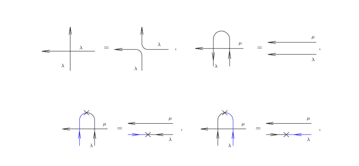
Figure 1. R-matrix properties

(all the crossing relations remain true if the horizontal line is blue (anti-fundamental)) and the conjugation identities (2.4) are depicted in Fig. 1 and Fig. 2.

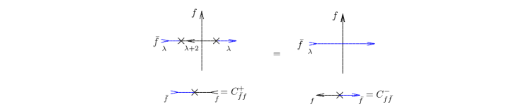
Figure 2. Crossing relations

Let us start with a more general case of the construction which is used for the introduction of temperature (see for example the book [47]). We consider a lattice which contains an additional direction, sometimes called the Matsubara direction as was discussed in paper [20]. Periodic boundary conditions in both, vertical and horizontal, directions are implied. So, we take $2N$ lattice sites in the Matsubara direction, where the corresponding horizontal lines are taken in staggered order as it is shown in Fig. 3, [48, 49, 50].

Obviously, we can depict the $n$-site density matrix $D^{i_{1}^{\prime}\dots i_{n}^{\prime}}_{i_{1}\dots i_{n}}(\lambda_{1},\dots,\lambda_{n})$ as shown on Fig. 3.

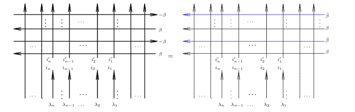
Figure 3. Introducing the anti-fundamental representation

Due to periodic boundary conditions in both, vertical and horizontal, directions, the lines form closed loops, except the lines with the cut. The density matrix acts onto $n$-sites quantum operators that graphically can be inserted into the cut with edges $i_{1},\dots,i_{n},i_{1}^{\prime},\dots,i_{n}^{\prime}$. All transfer matrices commute, so we can change the line order every moment. The horizontal (the auxiliary spaces) lines correspond to usual transfer matrices $T(\lambda)$, and the vertical (the quantum spaces) ones correspond to the quantum transfer matrices. Let us set $\beta=1/(2TN)$, where $T$ is the temperature. We intend to work with the zero temperature case, so we must be careful with the limit $N\rightarrow\infty$. The normalization to the highest eigenvalue is implied for all the transfer matrices $T(\lambda)$. We will come to this point later.

The $N$ lines going from the left to the right can be rewritten using the crossing relations (2.4) and associated anti-fundamental representations in such a way that all $2N$ horizontal lines go from the right to the left, where $N$ lines correspond to the fundamental representation, and the other $N$ lines correspond to the anti-fundamental representation, as shown in Fig. 3.

In the spirit of the paper [20], we can consider a more general case with two sets of arbitrary spectral parameters $\{\beta_{j}\},\{\bar{\beta}_{j}\},j=1,\cdots N$, associated with $N$ “fundamental lines” and $N$ “anti-fundamental lines”, respectively.

Then we can deduce two kinds of relations: one set for the case when $\lambda_{1}=\beta_{j},j=1,\cdots N$ and another set for $\lambda_{1}={\bar{\beta}}_{j},j=1,\cdots N$. Since the transfer matrices corresponding to horizontal lines commute, we can take any fixed number $j$ for our derivation without any loss of generality. After further manipulations shown in Fig. 5–Fig. 6, we will come to a couple of two relations which connect two objects earlier shown in Fig. 4:

$$D^{(0)}(\lambda_{1},\ldots,\lambda_{n}|\beta_{1},\ldots,\beta_{N};\bar{\beta}_{1},\ldots,\bar{\beta}_{N})\qquad{\mathrm{and}}\qquad D^{(1)}(\lambda_{1},\ldots,\lambda_{n}|\beta_{1},\ldots,\beta_{N};\bar{\beta}_{1},\ldots,\bar{\beta}_{N}).$$

The first object $D^{(0)}$ corresponds to the situation, where the fundamental representation is assigned to all vertical lines. The second object $D^{(1)}$ corresponds to the situation with one “anti-fundamental” vertical line taken for the space $1$, while all other vertical lines are “fundamental”.

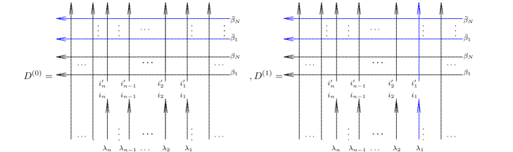
Figure 4. Two density matrices

Now we are going to prove that these density matrices satisfy the equations shown in Fig. 7 and Fig. 8. The relations can easily be established using pictures. A single action of the $A^{(1)}$-operator (see definition (4.3)) onto the matrix $D^{(0)}$ can be shown by Fig. 5.

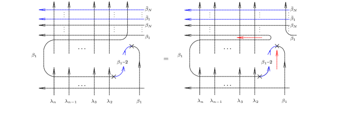
Figure 5. Relation for $D^{(0)}$

Here we use initial condition $R(0)=P$. In order not to overload pictures, let us omit all the quantum spaces here except those containing the cut, but keep in mind their existence. In the last expression we can make a few transformations. Firstly, we move the left “curve” through all the vertical lines (see red arrow on the picture). We can do it just using the unitarity relation for the $R$-matrices. Next, using the crossing relations (2.8, (2.9), we move the remaining “curve” through all the horizontal lines in vertical direction (see the red arrow), then such a loop comes back in the bottom due to the cyclicity, and also one additional vertical line appears.

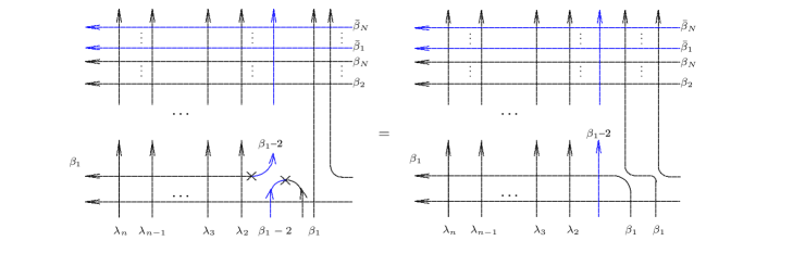
Figure 6. Relation for $D^{(1)}$

Now let us use again the initial condition Fig. 1 in order to obtain the final expression. At the last step we use the initial condition two times more for the last three lines, and the density matrix restores automatically at the right-hand side of the relation. Formally, there is a problem concerning two additional quantum spaces that appear in the final expression. But actually, this is not a problem because at the end we send the number of the quantum spaces to infinity (thermodynamic limit), and so, the few additional lines do not change anything if they are properly normalized. In our case we have to normalize two additional vertical lines. It causes the appearance of the factor $\Lambda(\beta_{1})\bar{\Lambda}(\beta_{1}-2)$. Here $\Lambda(\lambda)$ and $\bar{\Lambda}(\lambda)$ are maximal eigenvalues of the quantum transfer matrices corresponding to fundamental and anti-fundamental representations, respectively. Fortunately, the above factor is just equal to $1$. Therefore, we get the correct normalization automatically.

Finally, we obtain the relation depicted in Fig. 7.

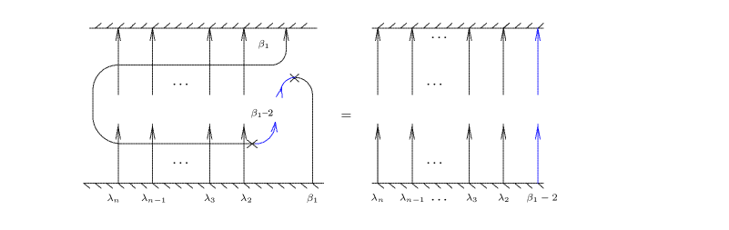
Figure 7. First difference equation

As we already pointed out, the set of quantum spaces without cut are implied, but they are not shown in the picture. Now we denote an infinite set of auxiliary spaces just by the grounding.

We wish to stress that on the right-hand side of the relation we get the matrix
$D^{(1)}(\lambda_{1},\ldots,\lambda_{n}|\beta_{1},\ldots,\beta_{N};\bar{\beta}_{1},\ldots,\bar{\beta}_{N})$ with the proper shift of spectral parameter and with one anti-fundamental line corresponding to the first quantum space. Meanwhile on the left hand side we have the matrix $D^{(0)}(\lambda_{1},\ldots,\lambda_{n}|\beta_{1},\ldots,\beta_{N};\bar{\beta}_{1},\ldots,\bar{\beta}_{N})$ we started with.

In a similar way we can obtain the second equation using the operator (4.4) and $D^{(1)}$ (see Fig. 8).

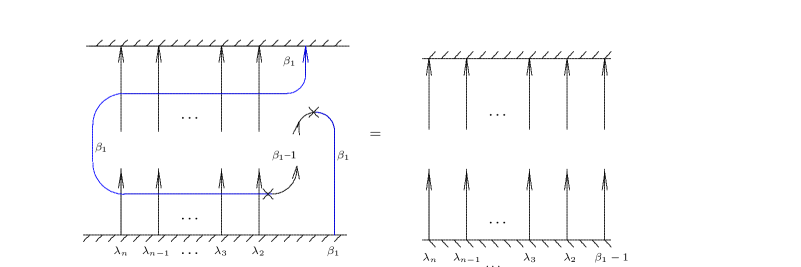
Figure 8. Second difference equation

Then we have the density matrix $D^{(1)}(\lambda_{1},\ldots,\lambda_{n}|\beta_{1},\ldots,\beta_{N};\bar{\beta}_{1},\ldots,\bar{\beta}_{N})$ on the left-hand side and $D^{(0)}(\lambda_{1},\ldots,\lambda_{n}|\beta_{1},\ldots,\beta_{N};\bar{\beta}_{1},\ldots,\bar{\beta}_{N})$ on the right-hand side of our relation.

Finally, we come to the following two equations:

$$D^{(0)}(\beta_{j},\lambda_{2},\ldots,\lambda_{n}|\beta_{1},\ldots,\beta_{N};\bar{\beta}_{1},\ldots,\bar{\beta}_{N})\Bigl{(}A^{(1)}_{1,\bar{1}|2,\ldots,n}(\beta_{j}|\lambda_{2},\ldots,\lambda_{n})\bigl{(}X_{\bar{1},2,\ldots,n}\bigr{)}\Bigr{)}\\ =D^{(1)}(\beta_{j}-2,\lambda_{2},\ldots,\lambda_{n}|\beta_{1},\ldots,\beta_{N};\bar{\beta}_{1},\ldots,\bar{\beta}_{N})\bigl{(}X_{\bar{1},2,\ldots,n}\bigr{)},$$ (A.1)

$$D^{(1)}({\bar{\beta}}_{j},\lambda_{2},\ldots,\lambda_{n}|\beta_{1},\ldots,\beta_{N};\bar{\beta}_{1},\ldots,\bar{\beta}_{N})\Bigl{(}A^{(2)}_{\bar{1},1|2,\ldots,n}({\bar{\beta}}_{j}|\lambda_{2},\ldots,\lambda_{n})\bigl{(}X_{1,\ldots,n}\bigr{)}\Bigr{)}\\ =D^{(0)}({\bar{\beta}}_{j}-1,\lambda_{2},\ldots,\lambda_{n}|\beta_{1},\ldots,\beta_{N};\bar{\beta}_{1},\ldots,\bar{\beta}_{N})\bigl{(}X_{1,\ldots,n}\bigr{)}.$$ (A.2)

Let us comment on the above relations (A.1), (A.2) (see also Fig. 7 and Fig. 8). Actually, we would not call them rqKZ equations since they are not really difference relations. The expressions standing on the left- and on the right-hand side are essentially different because the first argument of $D^{(0)}$ and $D^{(1)}$, $\beta_{j}$ or $\bar{\beta}_{j}$ respectively, is shifted on the right-hand side of (A.1), (A.2), but there is also dependence on the non-shifted parameters within both sets $\{\beta_{j}\},\{\bar{\beta}_{j}\}$, while on the left-hand side of (A.1), (A.2) the first argument is not shifted. It means that relations (A.1), (A.2) are not closed.

Let us see that in the zero temperature limit we will come to real difference relations. So, we set again $\beta_{k}\to\frac{1}{2TN}$ and ${\bar{\beta}}_{k}\to 1-\frac{1}{2TN}$ for $k=1,\cdots,N$ and then take the so-called Trotter limit $N\to\infty$ [49]. Finally, we have to take the limit $T\to 0$.

Let us make one important remark here. We could start with the situation where the whole number of quantum spaces in horizontal direction is finite, say, $L$. We are interested in taking the limit when both $L$ and $N$ tend to infinity. In paper [20] the limit $L\to\infty$ was taken first. Let us assume that both limits commute. So, if we first take the limit $L\to\infty$ keeping the Trotter number $N$ finite, we can insert the projector to the ground state somewhere at the right or at the left infinity in the vertical direction. We see that in this case all vertical lines except $n$ lines, where the cut is taken disappear if they are properly normalized by the maximal eigenvalue of the corresponding quantum transfer matrices as we discussed above. On the other hand, if we take the limit $N\to\infty$, $T\to 0$ first keeping $2TN=1/\lambda_{1}$ and $L$ finite (with some arbitrary parameter $\lambda_{1}$), we can insert the projector to the vacuum somewhere at infinity in the horizontal direction. Then the horizontal lines will disappear. Again we have to normalize them by putting the maximal eigenvalue into the denominator. Because of the duality of both pictures we can realize that both ways of normalization are compatible with each other. We have checked numerically that the above scheme actually works well (see Tables 1 and 2).

So, we come to the vacuum expectation value (3.1):

$$D^{(0)}(\beta_{j},\lambda_{2},\ldots,\lambda_{n}|\beta_{1},\ldots,\beta_{N};\bar{\beta}_{1},\ldots,\bar{\beta}_{N})\bigl{(}X_{\bar{1},2,\ldots,n}\bigr{)}\to D(\lambda_{1},\ldots,\lambda_{n})\bigl{(}X_{\bar{1},2,\ldots,n}\bigr{)},$$

$$D^{(1)}(\beta_{j},\lambda_{2},\ldots,\lambda_{n}|\beta_{1},\ldots,\beta_{N};\bar{\beta}_{1},\ldots,\bar{\beta}_{N})\bigl{(}X_{1,2,\ldots,n}\bigr{)}\to D^{(1)}(\lambda_{1},\ldots,\lambda_{n})\bigl{(}X_{1,2,\ldots,n}\bigr{)}$$

with the original generalized density matrix $D$ defined by (3.3) and $D^{(1)}$ can be defined in a similar way by taking the anti-fundamental representation for the first line.

Now, as was explained in Section 4, we can combine equations (A.1), (A.2) and get finally the closed equation with the same matrix $D$ at both sides (see 4.5). The corresponding diagram is shown in Fig. 9 .

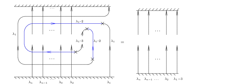
Figure 9. rqKZ equation

Appendix B Some details on formula (4.69)

In this Appendix we explain some details of our derivation of formula (4.69) from Section 4.4. Let us start with the functional relation (4.56). Then we can substitute formula (4.28) for the function $\bar{\omega}^{(1)}$ into the right-hand side of (4.56) using formula (4.57) for the function $r(\lambda)$. Applying partial fraction decomposition, we can write it in the following form:

$$r(\lambda)=\sum\limits_{j\geq 0}s_{j}(\lambda)\\ -\frac{1}{256}\Bigl{(}\frac{3/5}{(\lambda-4)^{2}}+\frac{3}{(\lambda-2)^{2}}-\frac{3}{(\lambda-1)^{2}}-\frac{3/5}{(\lambda+1)^{2}}-\frac{1}{\lambda-4}+\frac{1}{\lambda-2}+\frac{1}{\lambda-1}-\frac{1}{\lambda+1}\Bigr{)}\bar{\omega}^{(1)}(0)\\ -\frac{1}{384}\Bigl{(}\frac{3/5}{(\lambda-4)^{2}}-\frac{1}{(\lambda-2)^{2}}-\frac{10}{(\lambda-1)^{2}}+\frac{2/5}{(\lambda+1)^{2}}-\frac{19/15}{\lambda-4}+\frac{13}{\lambda-2}-\frac{34/3}{\lambda-1}-\frac{2/5}{\lambda+1}\Bigr{)},$$ (B.1)

where

$$s_{j}(\lambda)=\frac{b_{2,0,j}}{(\lambda-3j)^{2}}-\frac{b_{2,0,j+1}}{(\lambda+3j)^{2}}+\frac{b_{2,1,j}}{(\lambda-1-3j)^{2}}-\frac{b_{2,1,j+1}}{(\lambda+1+3j)^{2}}\\ +\frac{b_{1,0,j}}{\lambda-3j}+\frac{b_{1,0,j+1}}{\lambda+3j}+\frac{b_{1,1,j}}{\lambda-1-3j}+\frac{b_{1,1,j+1}}{\lambda+1+3j}\\ +\frac{a_{2,4,j}}{(\lambda-4)^{2}}+\frac{a_{2,2,j}}{(\lambda-2)^{2}}+\frac{a_{2,1,j}}{(\lambda-2)^{2}}+\frac{a_{2,1,j}}{(\lambda-1)^{2}}+\frac{a_{2,-1,j}}{(\lambda+1)^{2}}+\frac{a_{2,-1,j}}{(\lambda-1)^{2}}+\frac{a_{2,-1,j}}{(\lambda-1)^{2}},$$ (B.2)

and

$$b_{2,0,j}=\frac{1}{64}\Bigl{(}-\frac{2/5}{3j-4}+\frac{2/5}{3j+1}-\frac{1}{3j-2}+\frac{1}{3j-1}\Bigr{)},$$

$$b_{2,1,j}=\frac{1}{64}\Bigl{(}\frac{2/5}{3j-3}-\frac{2/5}{3j+2}+\frac{1}{3j-1}-\frac{1}{3j}\Bigr{)},$$

$$b_{1,0,j}=\frac{1}{64}\Bigl{(}\frac{4/5}{(3j-4)^{2}}-\frac{4/5}{(3j+1)^{2}}+\frac{2}{(3j-2)^{2}}-\frac{2}{(3j-1)^{2}}+\frac{1}{3j-4}+\frac{1}{3j+1}-\frac{1}{3j-2}-\frac{1}{3j-1}\Bigr{)},$$

$$b_{1,1,j}=\frac{1}{64}\Bigl{(}-\frac{4/5}{(3j-3)^{2}}+\frac{4/5}{(3j+2)^{2}}-\frac{2}{(3j-1)^{2}}+\frac{2}{(3j)^{2}}-\frac{1}{3j-3}-\frac{1}{3j+2}+\frac{1}{3j-1}+\frac{1}{3j}\Bigr{)}$$

$$a_{2,4,j}=\frac{1}{160}\Bigl{(}-\frac{1}{3j-4}-\frac{1}{3j+4}+\frac{1}{3j+5}+\frac{1}{3j-3}\Bigr{)},$$

$$a_{2,2,j}=\frac{1}{64}\Bigl{(}-\frac{1}{3j-2}-\frac{1}{3j+2}+\frac{1}{3j+3}+\frac{1}{3j-1}\Bigr{)},$$

$$a_{2,1,j}=\frac{1}{64}\Bigl{(}-\frac{1}{3j-1}-\frac{1}{3j+1}-\frac{1}{3j+2}-\frac{1}{3j}\Bigr{)},$$

$$a_{2,-1,j}=\frac{1}{160}\Bigl{(}\frac{1}{3j+1}+\frac{1}{3j-1}-\frac{1}{3j+2}-\frac{1}{3j}\Bigr{)},$$

$$a_{1,4,j}=\frac{1}{80}\Bigl{(}-\frac{1}{(3j-4)^{2}}+\frac{1}{(3j+4)^{2}}-\frac{1}{(3j+5)^{2}}+\frac{1}{(3j-3)^{2}}\Bigr{)}$$

$$\hskip 85.35826pt+\frac{1}{64}\Bigl{(}-\frac{1}{3j-4}-\frac{1}{3j+4}+\frac{1}{3j+5}+\frac{1}{3j-3}\Bigr{)},$$

$$a_{1,2,j}=\frac{1}{64}\Bigl{(}-\frac{2}{(3j-2)^{2}}+\frac{2}{(3j+2)^{2}}-\frac{2}{(3j+3)^{2}}+\frac{2}{(3j-1)^{2}}$$

$$\hskip 85.35826pt+\frac{1}{3j-2}+\frac{1}{3j+2}-\frac{1}{3j+3}-\frac{1}{3j-1}\Bigr{)},$$

$$a_{1,1,j}=\frac{1}{64}\Bigl{(}\frac{2}{(3j-1)^{2}}-\frac{2}{(3j+1)^{2}}+\frac{2}{(3j+2)^{2}}-\frac{2}{(3j)^{2}}+\frac{1}{3j-1}+\frac{1}{3j+1}-\frac{1}{3j+2}-\frac{1}{3j}\Bigr{)},$$

$$a_{1,-1,j}=\frac{1}{80}\Bigl{(}\frac{1}{(3j+1)^{2}}-\frac{1}{(3j-1)^{2}}+\frac{1}{(3j)^{2}}-\frac{1}{(3j+2)^{2}}\Bigr{)}$$

$$\hskip 85.35826pt+\frac{1}{64}\Bigl{(}-\frac{1}{3j+1}-\frac{1}{3j-1}-\frac{1}{3j}+\frac{1}{3j+2}\Bigr{)}.$$ (B.3)

It is easy to check that

$$b_{2,0,0}=b_{2,0,1}=b_{1,0,0}=b_{1,0,1}=0.$$

Besides, it is implied that in the summation (B.1)

$$b_{2,1,0}=b_{2,1,1}=b_{1,0,0}=b_{1,0,1}=b_{1,1,0}=b_{1,1,1}=0.$$ (B.4)

From formulas (4.56), (B.1) we can deduce that the solution for $\bar{\bar{\omega}}^{(3)}$ has the following form:

$$\bar{\bar{\omega}}^{(3)}(\lambda) = \;\;\sum\limits_{j\geq 2}c_{2,0,j}\Bigl{(}\frac{1}{(\lambda-3j)^{2}}+\frac{1}{(\lambda+3j)^{2}}\Bigr{)}+c_{1,0,j}\Bigl{(}\frac{1}{\lambda-3j}-\frac{1}{\lambda+3j}\Bigr{)}$$

$$+\sum\limits_{j\geq 0}c_{2,1,j}\Bigl{(}\frac{1}{(\lambda-1-3j)^{2}}+\frac{1}{(\lambda+1+3j)^{2}}\Bigr{)}+c_{1,1,j}\Bigl{(}\frac{1}{\lambda-1-3j}-\frac{1}{\lambda+1+3j}\Bigr{)},$$

where

$$c_{2,0,j}=-\sum\limits_{k=2}^{j}b_{2,0,k},\qquad c_{1,0,j}=-\sum\limits_{k=2}^{j}b_{1,0,k},$$ (B.6)

$$c_{2,1,j}=-\sum\limits_{k=0}^{j}b_{2,1,k},\qquad c_{1,1,j}=-\sum\limits_{k=0}^{j}b_{1,1,k},$$

but we should correct the boundary values (B.4). We take

$$b_{2,1,j}=\begin{cases}a,&j=0\\ d+\frac{a}{5},&j=1\\ \frac{1}{64}\Bigl{(}-\frac{4/5}{(3j-3)^{2}}+\frac{4/5}{(3j+2)^{2}}-\frac{2}{(3j-1)^{2}}+\frac{2}{(3j)^{2}}-\frac{1}{3j-3}-\frac{1}{3j+2}+\frac{1}{3j-1}+\frac{1}{3j}\Bigr{)},&j\geq 2\end{cases}$$

$$b_{1,1,j}=\begin{cases}b,&j=0\\ c-\frac{2}{5}b,&j=1\\ \frac{1}{64}\Bigl{(}\frac{2/5}{3j-3}-\frac{2/5}{3j+2}+\frac{1}{3j-1}-\frac{1}{3j}\Bigr{)},&j\geq 2\end{cases}.$$

In Section 4.4 we defined the values of $a$ and $b$ by the formulas (4.73). Also we should define

$$c=\frac{2644-225\sqrt{3}\pi-2025\log{3}}{28800},$$ (B.8)

$$d=-\frac{77}{9600}.$$

One can check that with this definition one has the coinciding residues of the left- and right-hand sides of the functional relation (4.56) at all values $\lambda=3j,\;\pm 1+3j$, where $j=0,\pm 1,\pm 2,\cdots$. Explicitly one has from (B)

$$\bar{\bar{\omega}}^{(3)}(\lambda)=\bar{\bar{\omega}}^{(3)}(-\lambda).$$

Also one can see that it falls down at least as $1/\lambda^{2}$ when $\lambda\to\infty$. So, using the Liouville theorem we come to the conclusion that the solution (B) for $\bar{\bar{\omega}}^{(3)}(\lambda)$ is unique.

In order to come to the form (4.69), we can separate the sum on the right-hand side of (B) in two parts

$$\bar{\bar{\omega}}^{(3)}(\lambda)=I_{0}(\lambda)+I_{1}(\lambda),$$ (B.9)

where the summation in the first term $I_{0}$ goes from 2 to $\infty$ and the summation in the second term $I_{1}$ goes from 0 to 1.

So, we should take the corresponding parts of the function $r(\lambda)$ which stands at the right-hand side of (4.56). To this end we define three sums together with some boundary terms

$$r_{1}(\lambda):=\sum\limits_{j\geq 2}\Bigl{(}\frac{b_{2,0,j}}{(\lambda-3j)^{2}}-\frac{b_{2,0,j+1}}{(\lambda+3j)^{2}}\Bigr{)},$$

$$r_{2}(\lambda):=\sum\limits_{j\geq 2}\Bigl{(}\frac{b_{1,0,j}}{\lambda-3j}+\frac{b_{1,0,j+1}}{\lambda+3j}+\frac{b_{1,1,j}}{\lambda-1-3j}+\frac{b_{1,1,j+1}}{\lambda+1+3j}\Bigr{)}-\frac{c_{1,0,1}}{\lambda-6}-\frac{c_{1,0,2}}{\lambda+3}-\frac{c_{1,1,1}}{\lambda-7}-\frac{c_{1,1,2}}{\lambda+4},$$

$$r_{3}(\lambda):=\sum\limits_{j\geq 2}\Bigl{(}\frac{b_{2,1,j}}{(\lambda-1-3j)^{2}}-\frac{b_{2,1,j+1}}{(\lambda+1+3j)^{2}}\Bigr{)}+\frac{c_{2,1,2}}{(\lambda+4)^{2}}-\frac{c_{2,1,1}}{(\lambda-7)^{2}},$$

which can be calculated explicitly, for example, with the help of Mathematica. With this definition we get the equation

$$I_{0}(\lambda-3)-I_{0}(\lambda)=r_{1}(\lambda)+r_{2}(\lambda)+r_{3}(\lambda).$$

The sum of the functions $r_{1}(\lambda),r_{2}(\lambda),r_{3}(\lambda)$ is regular for $-7<{\rm Re\,}{\lambda}<4$. Hence, we can write down the above first term $I_{0}$ as an integral

$$I_{0}(\lambda) := -\int\limits_{-i\infty}^{i\infty}\frac{d\mu}{6i}\tan\Bigl{(}{\frac{\pi}{3}(\lambda-\mu)}\Bigr{)}S(\mu),$$ (B.10)

where the function $S$ in the integrand is

$$S(\lambda)=-S(-\lambda)=r_{1}(\lambda+\frac{3}{2})+r_{2}(\lambda+\frac{3}{2})+r_{3}(\lambda+\frac{3}{2}),$$ (B.11)

while the residual term $I_{1}$ is a rational function of $\lambda$

$$I_{1}(\lambda):=-a\Bigl{(}\frac{1}{(\lambda-1)^{2}}+\frac{1}{(\lambda+1)^{2}}\Bigr{)}+\Bigl{(}d+\frac{6}{5}a\Bigr{)}\Bigl{(}\frac{1}{(\lambda-4)^{2}}+\frac{1}{(\lambda+4)^{2}}\Bigr{)}\\ -b\Bigl{(}\frac{1}{\lambda-1}-\frac{1}{\lambda+1}\Bigr{)}-\Bigl{(}c+\frac{3}{5}b\Bigr{)}\Bigl{(}\frac{1}{\lambda-4}-\frac{1}{\lambda+4}\Bigr{)}.$$ (B.12)

The function $S(\lambda)$ in the above definition of the integral $I_{0}$ can be explicitly calculated:

$${\displaystyle S(\lambda):=\frac{\lambda(48\lambda^{4}-280\lambda^{2}+259)}{2\,d_{1}(\lambda)^{2}}\cdot\Bigl{(}\psi\Bigl{(}\frac{1}{2}+\frac{\lambda}{3}\Bigr{)}+\psi\Bigl{(}\frac{1}{2}-\frac{\lambda}{3}\Bigr{)}-\psi\Bigl{(}\frac{5}{6}+\frac{\lambda}{3}\Bigr{)}-\psi\Bigl{(}\frac{5}{6}-\frac{\lambda}{3}\Bigr{)}\Bigr{)}}\\ {\displaystyle+\frac{4\lambda^{2}-9}{48\,d_{1}(\lambda)}\cdot\Bigl{(}\psi_{1}\Bigl{(}\frac{1}{2}+\frac{\lambda}{3}\Bigr{)}-\psi_{1}\Bigl{(}\frac{1}{2}-\frac{\lambda}{3}\Bigr{)}-\psi_{1}\Bigl{(}\frac{5}{6}+\frac{\lambda}{3}\Bigr{)}+\psi_{1}\Bigl{(}\frac{5}{6}-\frac{\lambda}{3}\Bigr{)}\Bigr{)}}\\ {\displaystyle-\frac{2\,\lambda\,(68\lambda^{2}-617)}{5\,d_{2}(\lambda)}\cdot\Bigl{(}\psi_{1}\Bigl{(}\frac{1}{3}\Bigr{)}-\frac{5\pi^{2}}{6}\Bigr{)}+\frac{\lambda\,p_{1}(\lambda)}{5\,d_{2}(\lambda)^{2}}\cdot\Bigl{(}3\log{3}+\frac{\pi}{\sqrt{3}}\Bigr{)}+\frac{2\,\lambda\,p_{2}(\lambda)}{375\,d_{2}(\lambda)^{2}}}.$$ (B.13)

where

$$d_{1}(\lambda):=(2\lambda-5)\,(2\lambda-1)\,(2\lambda+1)\,(2\lambda+5),$$ (B.14)

$$d_{2}(\lambda):=(2\lambda-11)\,(2\lambda-5)\,(2\lambda-1)\,(2\lambda+1)\,(2\lambda+5)\,(2\lambda+11),$$

$$p_{1}(\lambda):=256\,\lambda^{8}-54528\,\lambda^{6}+1190496\,\lambda^{4}-5423440\,\lambda^{2}+4738305,$$

$$p_{2}(\lambda):=18032\,\lambda^{4}-759448\,\lambda^{2}+5395775.$$

If the argument $\lambda$ is purely imaginary, $\lambda=ix$ with $x\in{\rm Re\,}$, the function $S(\lambda)$ is purely imaginary as well. The behavior of the imaginary part ${\rm Im\,}{(S(ix))}$ is shown in Fig. 10. At infinity it approaches 0 as $x^{-3}$. Hence, the integral (B.10) is convergent.

It is important that the function $S(\lambda)$ is regular in the interval $-11/2<{\rm Re\,}{\lambda}<11/2$. It guarantees that we can shift the integration contour by $\pm 3$ in the integral (B.10) along the real axis without catching any singularities that would come from the function $S$. There is only one contribution that comes from the residue at $\mu=\lambda-3/2$ where the function $\tan(\pi/3(\lambda-\mu))$ has a pole. It provides a non-trivial result for the difference $I_{0}(\lambda-3)-I_{0}(\lambda)$. We imply here that the integral with shifted argument $I_{0}(\lambda-3)$ must be determined as analytical continuation of $I_{0}(\lambda)$. It means that together with the shift of the spectral parameter $\lambda$ also the integration contour should be shifted by -3 along the real axis.

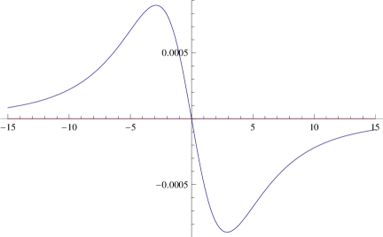
Figure 10. Behavior of the function ${\rm Im\,}(S(ix))$

Finally, we can check that the solution (B.9) indeed satisfies the functional equation (4.56).

Actually, we can explicitly take the integral for the rational part of the function $S(\lambda)$ in (B.10) and combine it with the term $I_{1}(\lambda)$. After some algebra we can bring the sum of the terms $I_{0}$ and $I_{1}$ to the form (4.69). Actually, the function $s(\lambda)$ defined in (4.70) exactly corresponds to the part of the function $S(\lambda)$ (B.13) which depends on the functions $\psi$ and $\psi_{1}$.

As discussed in Section 4.4, the integral representation (B.10) that we derived here is useful for the study of the asymptotic behavior when the spectral parameter $\lambda$ is close to $0$. Unfortunately, it does not seem very useful for the investigation of asymptotic behavior at large $|\lambda|\to\infty$. Although our numerical study supports the expected behavior (4.62), for the moment we cannot approve it analytically. We seem to need some other integral representation. So, we leave this question for future consideration.

Acknowledgements. The authors are grateful to A. Isaev, A. Klümper, A. Razumov, G. Ribeiro and F. Smirnov for many stimulating discussions. Our special thanks go to F. Göhmann for careful reading of the manuscript and many useful suggestions. AH is grateful to J. Sirker and A. Weiße for advises concerning numerical calculations.

The authors would like to thank Deutsche Forschungsgemeinschaft for support within the framework of the DFG Forschergruppe FOR 2316, projects number BO 3401/1-1 and GO 825/8-1. The work of Kh.S.N. was supported in part by the RFBR grant # 16-01-00473 and by the Russian Academic Excellence Project ’5-100’.

Note added: After our paper appeared on the arXiv, we became aware of the related preprint [51].

References

[1]
H. Boos, J. Damerau, F. Göhmann, A. Klümper, J. Suzuki, and A. Weiße,
Short-distance thermal correlations in the XXZ chain, J. Stat.
Mech.: Theor. Exp. (2008), P08010.
[2]
C. Trippe, F. Göhmann, and A. Klümper, Short-distance thermal
correlations in the massive XXZ chain, Eur. Phys. J. B73 (2010),
253–264.
[3]
J. Sato, B. Aufgebauer, H. Boos, F. Göhmann, A. Klümper, M. Takahashi, and
C. Trippe, Computation of static Heisenberg-chain correlators:
Control over length and temperature dependence, Phys. Rev. Lett.106 (2011), 257201–04.
[4]
Ph. Di Francesco and F. Smirnov,
OPE for XXX, Rev. Math. Phys.30 (2018) 184006;
arXiv:1711.04123 [hep-th].
[5]
T. Miwa and F. Smirnov,
New exact results on density matrix for XXX spin chain,
arXiv:1802.08491 [math-ph].
[6]
N. Kitanine, K. K. Kozlowski, J. M. Maillet, N. A. Slavnov, and V. Terras,
Algebraic Bethe ansatz approach to the asymptotic behavior of
correlation functions, J. Stat. Mech.: Theor. Exp.0904 (2009), P003.
[7]
M. Jimbo, K. Miki, T. Miwa, and A. Nakayashiki,
Correlation functions of the XXZ model for ,
Phys. Lett. A168 (1992), 256–263.
[8]
R. J. Baxter, Corner transfer matrices of the eight-vertex model. I.
Low-temperature expansions and conjectured properties, J. Stat. Phys.15 (1976), 485–503.
[9]
A. A. Belavin, A. M. Polyakov, and A. B. Zamolodchikov, Infinite
conformal symmetry in two-dimensional quantum field theory, Nucl. Phys. B241 (1984), 333–380.
[10]
M. Jimbo and T. Miwa, Quantum KZ equation with and
correlation functions of the XXZ model in the gapless regime, J. Phys. A29 (1996), 2923–2968.
[11]
I. Frenkel and N. Reshetikhin,
Quantum affine algebras and holonomic difference equations,
Comm. Math. Phys.146 (1992), 1–60.
[12]
F. A. Smirnov, Dynamical symmetries of massive integrable models.
1. Form factor bootstrap equations as a special case of deformed
Knizhnik–Zamolodchikov equations, Int. J. Mod. Phys. A7
(1992), 813–837.
by same author,
Dynamical symmetries of massive integrable models.
2. Space of states of massive models as space of operators,
Int. J. Mod. Phys. A7, Suppl. 1B (1992), 839–858.
[13]
N. Kitanine, J. M. Maillet, and V. Terras,
Correlation functions of the XXZ Heisenberg spin- chain in a magnetic field,
Nucl. Phys. B567 (1999), 554–582; arXiv:math-ph/9907019.
[14]
F. Göhmann, A. Klümper, and A. Seel, Integral representations for correlation functions
of the XXZ chain at finite temperature, J. Phys. A: Math. Gen, 37 (2004) 7625–7651;
hep-th/0405089
by same author, Integral representation of the density matrix of the XXZ chain at finite temperatures,
J. Phys. A: Math. Gen, 38 (2005), 1833–1841; arXiv:cond-mat/0412062.
[15]
H. Boos and V. Korepin,
Quantum spin chains and Riemann zeta function with odd arguments,
J. Phys. A: Math. Gen34 (2001), 5311–5316;
arXiv:hep-th/0104008.
by same author,
Evaluation of integrals representing correlations in XXX Heisenberg
spin chain, Prog. in Math. Phys.23, 65–108, in
MathPhys Odyssey 2001, ”Integrable Systems and Beyond”,
special issue in honor of Barry M. McCoy, edited by M. Kashiwara
and T. Miwa (Birkhäuser, Boston, 2001); arXiv:hep-th/0105144.
[16] M. Takahashi, Half-filled Hubbard model at low temperature,
J. Phys. C10 (1977), 1289–1301.
[17]
H. Boos, M. Jimbo, T. Miwa, F. Smirnov, and Y. Takeyama.
Hidden Grassmann structure in the XXZ model.
Comm. Math. Phys.272 (2007), 263–281.
[18]
H. Boos, M. Jimbo, T. Miwa, F. Smirnov, and Y. Takeyama.
Hidden Grassmann structure in the XXZ model II: Creation
operators.
Comm. Math. Phys.286 (2009), 875–932.
[19]
H. Boos, M. Jimbo, T. Miwa, and F. Smirnov, Completeness of a fermionic
basis in the homogeneous XXZ model, J. Math. Phys.50 (2009),
095206.
[20]
M. Jimbo, T. Miwa, and F. Smirnov.
Hidden Grassmann structure in the XXZ model III:
Introducing Matsubara direction.
J. Phys. A42 (2009) 304018 (31pp).
[21]
H. Boos and F. Göhmann, On the physical part of the factorized
correlation functions of the XXZ chain, J. Phys. A42 (2009),
315001.
[22]
V. Bazhanov, A. Hibberd, and S. Khoroshkin,
Integrable Structure of conformal field theory, quantum Boussinesq
theory and boundary affine Toda theory,
Nucl. Phys. B622 (2002), 475–574.
[23]
Z. Tsuboi,
Wronskian solutions of the and -systems related to infinite
diemnsional unitarizable modules of the general linear superalgebra ,
Nucl. Phys. B870 (2013), 92–137.
[24]
H. Boos, F. Göhmann, A. Klümper, Kh. S. Nirov, and A. V. Razumov,
Quantum groups and functional relations for higher rank,
J. Phys. A: Math. Theor., 47 (2014), 275201; arXiv:1312.2484 [math-ph].
[25]
C. N. Yang,
Some exact results for the many-body problem in one dimension with repulsive delta-function interaction,
Phys. Rev. Lett.19 (1967), 1312–1315.
[26]
B. Sutherland,
Further result for the many-body problem in one dimension,
Phys. Rev. Lett.20 (1968), 98–100.
[27]
B. Sutherland,
Model for a multicomponent quantum system,
Phys. Rev. B12 (1975), 3795–3805.
[28] P. Kulish and N. Reshetikhin,
Generalized Heisenberg ferromagnet and the Gross–Neveu
model, Zh. Eksp. Teor. Fiz.80 (1981), 214–231
(English version in Sov.Phys.JETP53 (1981) 108-114).
by same author, Diagonalisation of GL(N)
invariant transfer matrices and quantum N-wave system (Lee model),
J. Phys. A16 (1983), L591.
[29]
P. P. Kulish, Integrable graded magnets, J. Sov. Math.35 (1986),
2648–2662; [transl. from: Zap. Nauchn. Sem. LOMI145 (1985), 140–162
(in Russian)].
[30]
D. Gross and A. Neveu,
Dynamical symmetry breaking in asymptotically free field theories,
Phys. Rev. D10 (1974), 3235–3253.
[31]
E. Witten and R. Shankar,
The -matrix of the kinks of the model,
Nucl. Phys. B141 (1978), 349–363,
E. Witten,
Some properties of the model in two dimensions,
Nucl. Phys. B142 (1978), 285–300.
[32]
A. Zamolodchikov and Al. Zamolodchikov,
Exact S-Matrix of Gross-Neveu elementary fermions,
Phys. Lett. B72 (1978), 481–483,
by same author,
Relativistic factorized -matrix in two dimensions having isotopic symmetry,
Nucl. Phys. B133 (1978), 525–535,
by same author,
Factorized S-Matrices in two-dimensions as the exact solutions of certain
relativistic quantum field theory models,
Ann. Phys.120 (1979), 253–291.
[33]
H. Babujian, A. Foerster, and M. Karowski,
Exact form factors of the Gross-Neveu model and expansion,
Nucl. Phys. B825 (2010), 396–425.
[34]
R. Koberle, V. Kurak, and J. A. Swieca,
Scattering theory and expansion in the chiral Gross–Neveu model,
Phys. Rev. D20 (1979), 897–902;
B. Berg, M. Karowski, V. Kurak, and P. Weisz,
Factorized symmetric S matrices in two dimensions, Nucl. Phys. B134 (1978), 125–132.
[35]
F. Smirnov,
Form Factors in Completely Integrable Models of Quantum Field Theory,
Adv. Series in Math. Physics 14, World Scientific,
Singapore, (1992).
[36] S. Belliard, S. Pakuliak, E. Ragoucy, and N. A. Slavnov,
Form factors in SU(3)-invariant integrable models, J. Stat. Mech.1309
(2013), P04033, arXiv:1211.3968.
[37]
S. Pakuliak, E. Ragoucy, and N. A. Slavnov, Form factors in quantum
integrable models with GL(3)-invariant R-matrix, Nucl. Phys. B881 (2014), 343–368.
[38]
K. K. Kozlowski and E. Ragoucy, Asymptotic behaviour of two-point
functions in multi-species models, Nucl. Phys. B906 (2016), 241–288.
[39]
T. Kojima and S. Yamashita,
The critical chain,
J. Phys. A: Math. Gen.34 (2001), 1181–2001.
[40]
Y. Koyama, Staggered polarization of vertex models with -symmetry,
Commun. Math. Phys.164 (1994), 277–291; arXiv:hep-th/9307197.
[41]
H. Boos, V. Korepin, and F. Smirnov,
Emptiness formation probability and quantum Knizhnik-Zamolodchikov equation,
Nucl. Phys. B658 (2003), 417–439,
H. Boos, M. Jimbo, T. Miwa, F. Smirnov, and Y. Takeyama, A recursion formula for the correlation
functions of an inhomogeneous XXX model, Algebra and Analysis17 (2005), 115–159,
(Engl. version in St.Petersburg Math. J. 17 (2006), 85-117); arXiv:hep-th/0405044,
by same author,
Reduced qKZ equation and correlation functions of the XXZ model,
Comm. Math. Phys.261 (2006), 245–276; arXiv:hep-th/0412191,
by same author,
Density matrix of a finite sub-chain of the Heisenberg anti-ferromagnet,
Lett. Math. Phys.75 (2006), 201–208; arXiv:hep-th/0506171.
[42]
B. Aufgebauer and A. Klümper,
Finite temperature correlation functions from discrete functional equations,
J. Phys. A: Math. Theor.45 (2012), 345203.
[43]
V. N. Tolstoy and S. M. Khoroshkin,
The universal -matrix for quantum untwisted affine Lie algebras,
Funct. Anal. & Appl.26 (1992), 69-–71
[44]
H. Boos, F. Göhmann, A. Klümper, Kh. S. Nirov, and A. V. Razumov,
Exercises with the universal -matrix,
J. Phys. A: Math. Theor.43 (2010) 415208; arXiv:1004.5342 [math-ph].
[45]
S. M. Khoroshkin and V. N. Tolstoy,
Yangian double,
Lett. Math. Phys.36 (1994) 373–402;
Yangian double and rational -matrix, [arXiv:hep-th/9406194].
[46]
D. Martin and F. Smirnov,
Problems with using separated variables for computing expectation values for higher ranks,
Lett. Math. Phys.106 (2016), 469–484.
[47]
F. H. L. Eßler, H. Frahm, F. Göhmann, A. Klümper, and V. E. Korepin,
The one-dimensional Hubbard model, Cambridge University Press, (2005).
[48]
M. Suzuki,
Transfer-matrix method and Monte Carlo simulation in quantum spin systems,
Phys. Rev. B31 (1985), 2957–2965.
[49]
M. Takahashi,
Correlation length and free energy of the XYZ chain,
Phys. Rev. B43 (1991), 5788–5797; Erratum: ibid.44 (1991), 5397;
by same author,
Correlation length and free energy of the XXZ chain in a magnetic field,
Phys. Rev. B44 (1991), 12382–12394.
[50]
A. Klümper,
Thermodynamics of the anisotropic spin-1/2 Heisenberg chain and related quantum chains,
Z. Phys. B91 (1993), 507–519; arXiv:cond-mat/9306019.
[51]
G. A. P. Ribeiro and A. Klümper,
Correlation functions of the integrable spin chain,
arXiv:1804.10169 [math-ph].