Particle-filtering approaches for nonlinear Bayesian decoding of neuronal spike trains

Anna Kutschireiter ^1,2,3, Jean-Pascal Pfister ^1,2,3
1Institute of Neuroinformatics, UZH / ETH Zurich, Winterthurerstrasse 190, 8057 Zurich, Switzerland.
²Neuroscience Center Zurich (ZNZ), UZH / ETH Zurich, Winterthurerstrasse 190, 8057 Zurich, Switzerland.
³Department of Physiology, University of Bern, Bühlplatz 5, 3012 Bern, Switzerland.

Keywords:

Abstract

The number of neurons that can be simultaneously recorded doubles every seven years [1]. This ever increasing number of recorded neurons opens up the possibility to address new questions and extract higher dimensional signals or stimuli from the recordings. Modeling neural spike trains as point processes, this task of extracting dynamical analog signals from spike trains is commonly set in the context of nonlinear filtering theory. Particle filter methods relying on importance weights are generic algorithms that solve the filtering task numerically, but exhibit a serious drawback when the problem dimensionality is high: they are known to suffer from the ‘curse of dimensionality’ (COD), i.e. the number of particles required for a certain performance scales exponentially with the observable dimensions. Here, we first briefly review the theory on filtering and system identification with point process observations in continuous time. Based on this theory, we investigate both analytically and numerically the reason for the COD of weighted particle filtering approaches: Similarly to particle filtering with continuous-time observations, the COD with point-process observations is due to the decay of effective number of particles, an effect that is stronger when the number of observable dimensions increases. Given the success of unweighted particle filtering approaches in overcoming the COD for continuous-time observations, we introduce an unweighted particle filter for point-process observations, the spike-based Neural Particle Filter (sNPF), and show that it exhibits a similar favorable scaling as the number of dimensions grows. Further, we derive rules for the parameters of the sNPF from a maximum likelihood approach learning, that allows both online and offline unsupervised learning. We finally employ a simple decoding task to illustrate the capabilities of the sNPF and to highlight one possible future application of our inference and learning algorithm.

1 Introduction

Our nervous system represents information about the environment through coordinated spiking activity of neuronal populations. In the last decades, multiple electrodes have become standard tools in neuroscience research, registering the spiking activity of many neurons within and across different brain regions simultaneously. Presently, state-of-the-art probes offer the possibility to record up to 700 neurons at the same time [2]. On the one hand, this opens up new possibilities for applications, for instance in the design and implementation of brain-machine interfaces and neuroprostethic devices [3, 4]. On the other hand, analysis of this immense amount of data require algorithms that scale according to this high-dimensional input.

The theory of point processes allows to model and analyse time series of discrete, possibly probabilistic events [5], such as the spiking behavior of neurons in response to a stimulus or a combination of stimuli. The task of decoding is to reconstruct the stimulus from neuronal responses, which may be seen as restricted and noisy sensors. This task naturally has to be performed by neurons, which need to estimate their environmental state, as well as by experimenters if the ground truth of the stimulus is inaccessible. This is the case for example when decoding motor commands for prosthetics [3] or when decoding the ’position’ of an animal from place cell activities during memory recall [6]. Algorithms based on Bayesian statistics offer a general approach to decoding stimuli, or ‘states’, from neuronal activity, thereby taking into account prior knowledge about the stimulus in terms of a statistical representation [7, 8, 9, 10, 11, 12, 13].

If the stimulus is dynamic, then Bayesian decoding of the stimulus from the history of spikes can be framed in the context of filtering theory. The formal solution to the filtering problem with point process observations is infinite dimensional and thus, beyond specific settings, impossible to write down in closed form [14, 5]. Algorithms relying on a Gaussian approximation of the filtering distribution are abundantly used e.g. for decoding the position of animals from place cell activity [7, 15, 16] (here commonly referred to: Gaussian assumed density filters, ADF). However, these models are not able to capture multi-modal posteriors, which may occur for certain nonlinear stimulus dynamics and/or boundary conditions [17]. If the state space is discrete, a closed-form solution exists, which was used to model how filtering could be performed by a neuronal population [18, 19], and which could in principle also account for the decoding task. However, for continuous stimuli these approaches would depend on a discretization of state-space, which is disadvantageous if it is unconstrained or if its dimensionality is large.

Particle filters (PFs, cf. [20]) are a large class of algorithms that solve the filtering problem numerically. By approximating the posterior with a finite number of weighted empirical samples (so-called ‘particles’), PFs can accommodate a wide range of state-space models, and are, unlike for instance a Kalman filter [21, 22], not restricted to linear models. Particle filters have received some attention in the context of spike-train decoding [23, 24], but are known to suffer from the so-called ‘curse of dimensionality’ (COD): as the dimensionality of the problem increases, so does the demand in number of particles in order to keep the numerical performance on a satisfactory level. For continuous-time observations, it can be shown [25] that the COD manifests itself in a decreased decay time-scale of the particles’ importance weights. For point-process observations, the situation can be considered more severe, because the posterior distribution exhibits jumps.

Closely linked to, and in fact a prerequisite for effective decoding, is the encoding task, i.e. finding the relationship of stimulus and spike generation, for instance in terms of an instantaneous firing rate. In the context of point processes, encoding would refer to finding a model that relates the hidden state as well as the history of events with the point process observation. Encoding has been studied extensively (for review, see [12]), and mostly focuses on offline estimation [12] and/or settings where the stimulus is known [26]. However, it is known that we can expect plasticity of neural dynamics even on the time scales of a single recording session [27]. Place cells, for instance, change their respective place fields rapidly when an animal is placed in a new environment, more slowly in response to exploration [28] or as a result of external manipulation [29]. However, access to the ground-truth stimulus is not always possible, which justifies the need to formulate an encoding algorithm that is both online and unsupervised.

In this paper, we introduce an ansatz for a Bayesian decoding algorithm, the spike-based Neural Particle Filter (sNPF), that consists of a particle filter with equally weighted samples and builds on earlier work [30] to account for point process observations. The advantages of this filter are that it is formulated in continuous time and continuous-state space. Further, in its most general form it can accommodate any nonlinear hidden dynamics and encoding model, without the need to rely on Gaussian approximations, giving it a large flexibility with respect to models and boundary conditions. We demonstrate the performance of this filter in first a simple, one-dimensional toy model, and second, a more sophisticate model motivated by decoding the position of a foraging animal from hippocampal place cell responses. For the latter, we show that it outperforms state-of-the-art decoding decoding methods [16, 31], which are based on a Gaussian approximation, and that its performance is close to optimal. Further, we show that in contrast to standard weighted particle filters, the sNPF is able to avoid the COD, making it a suitable candidate for decoding of high-dimensional models. Based on a maximum-likelihood approach, the filter can be used to approximate the incomplete-data likelihood function. From this likelihood function, online learning rules for system identification can be derived, which may be useful for adaptive encoding when the stimulus is unknown.

2 Problem formulation

2.1 Generative model

Consider $m$ neurons whose spiking behavior is modeled by a Poisson point process [5] $\mathbf{N}_{t}=\{N_{t}^{(1)},\dots,N_{t}^{(m)}\}$, where $N_{t}^{(i)}$ counts the number of spikes of neuron $i$ that occurred in the time interval $[0,t)$. Equivalently, the trajectory of this process can be characterized by the sequence of its stochastic increments with $dN_{t}^{(i)}=1$ if neuron $i$ has elicited a spike at time $t$, and $dN_{t}^{(i)}=0$ otherwise. These increments are drawn from a Poisson distribution:

$$d\mathbf{N}_{t} \sim \text{Poisson}(d\mathbf{N}_{t};\,\mathbf{g}(\mathbf{x}_{t},\mathbf{N}_{0:t},t)\,dt).$$ (1)

Here, the instantaneous firing rate $\mathbf{g}(\mathbf{x}_{t},\mathbf{N}_{0:t},t)$ captures the biophysics that enter the firing of the neuron, for instance the dependence on an external stimulus $\mathbf{x}_{t}$, self-interaction and spiking history dependence such as refractoriness or interaction within the neuronal population. Since the firing rate $\mathbf{g}(\mathbf{x}_{t},\mathbf{N}_{t},t)$ defines the relationship between the stimulus $\mathbf{x}_{t}$ and the firing statistics of the neurons, it defines an encoding model, which we consider known.

We further consider a continuous-valued external stimulus $\mathbf{x}_{t}\in\mathbb{R}^{n}$ that evolves in time, the dynamics of which obeying the Itô stochastic differential equation (SDE):

$$d\mathbf{x}_{t} = \mathbf{f}(\mathbf{x}_{t})\,dt+\Sigma_{x}^{1/2}(\mathbf{x}_{t})d\mathbf{w}_{t},$$ (2)

where $\mathbf{f}(\mathbf{x}_{t}):\mathbb{R}^{n}\to\mathbb{R}^{n}$ denotes a potentially nonlinear drift term, $\mathbf{w}_{t}\in\mathbb{R}^{n}$ denotes a Brownian motion process and $\Sigma_{x}^{1/2}(\mathbf{x}_{t}):\mathbb{R}^{n}\to\mathbb{R}^{n\times n}$ is the diffusion term. In accordance with the mathematical filtering literature, we will refer to this process as the “(hidden) state”.

As an example consider a mouse moving freely in a specified environment, while at the same time the spike train of $m$ place cells is recorded. The position of the mouse at time $t$ is given by $\mathbf{x}_{t}$, which gives rise to the place cell activity via the instantaneous firing rate $\mathbf{g}(\mathbf{x}_{t},\mathbf{N}_{0:t},t)$. In the simplest case of no neuronal interaction, $g^{(i)}(\mathbf{x}_{t},\mathbf{N}_{0:t},t)=\lambda^{(i)}(\mathbf{x}_{t})$ would correspond to the place field or spatial tuning curve of neuron $i$. The spike train corresponds to the observations. The dynamics of the mouse is given in Eq. (2). Here, the stochastic diffusion term models the erratic behavior of the mouse, e.g. during forage, and the nonlinearity in the drift term $\mathbf{f}(\mathbf{x}_{t})$ may model specific attractors or repellers in the environment, such as food sources or averse stimuli. If the drift term is zero, the mouse performs a random walk. Note that for certain drift functions $\mathbf{f}(\mathbf{x}_{t})$ or spatial boundary conditions, Eq. (2) gives rise to a stationary probability distribution, which, together with the time scale of the movement, serves as prior knowledge. We will elaborate on this toy model further in section 4.

2.2 Decoding

For this example, the (online) decoding task would read: given the knowledge about the dynamics of the mouse, and given the knowledge about the place fields, what is the position of the mouse at time $t$ given the spike trains of the neurons up to this time.

More formally, we can frame decoding a nonlinear filtering problem: Given the model in Eqs. (1) and (2) and given the sequence of point-process observations $\mathbf{N}_{0:t}$, what is the posterior probability distribution (or filtering distribution) $p(\mathbf{x}_{t}|\mathbf{N}_{0:t})$. Equivalently, a full probabilistic solution to the filtering problem is known if the posterior expectation of any real-valued, measurable function $\phi$ can be computed:

$$\langle\phi(\mathbf{x}_{t})\rangle:=\mathbb{E}[\phi(\mathbf{x}_{t})|\mathbf{N}_{0:t}] = \int d\mathbf{x}_{t}\,\phi(\mathbf{x}_{t})p(\mathbf{x}_{t}|\mathbf{N}_{0:t}).$$ (3)

A formal solution for the evolution of this posterior expectation $\langle\phi_{t}\rangle$ can be written down in terms of an SDE [5, T7, p. 173]:

$$d\langle\phi_{t}\rangle = \langle\mathcal{L}[\phi_{t}]\rangle\,dt+\text{cov}(\phi_{t},\mathbf{g}_{t}^{T})\text{diag}\left(\langle\mathbf{g}_{t}\rangle\right)^{-1}\left(d\mathbf{N}_{t}-\langle\mathbf{g}_{t}\rangle\,dt\right),$$ (4)

where $\mathcal{L}[\phi_{t}]:=\sum_{i}f_{i}(\mathbf{x}_{t})\frac{\partial}{\partial x_{i}}\phi_{t}+\sum_{i,j}(\Sigma_{x}^{1/2})_{ij}\frac{\partial^{2}}{\partial x_{i}\partial x_{j}}\phi_{t}$ is the infinitesimal generator of the hidden process in Eq. (2). This solution suffers from a closure problem, i.e. it is analytically intractable, which can be seen when writing down the SDE for the first posterior moment, with $\phi(\mathbf{x}_{t})=\mathbf{x}_{t}$:

$$d\langle\mathbf{x}_{t}\rangle = \langle\mathbf{f}(\mathbf{x}_{t})\rangle\,dt+\text{cov}(\mathbf{x}_{t},\mathbf{g}_{t}^{T})\text{diag}\left(\langle\mathbf{g}_{t}\rangle\right)^{-1}\left(d\mathbf{N}_{t}-\langle\mathbf{g}_{t}\rangle\,dt\right),$$ (5)

which clearly depends on higher-order posterior moments. In general, any SDE for posterior moments will depend on higher-order moments.

Note that filtering usually asks for the full statistical description, while for decoding one would have to specify how the state estimate $\hat{\mathbf{x}}_{t}$ is obtained from this description. Here, by decoding we refer to determining the full posterior density of the state $\mathbf{x}_{t}$.

3 The sNPF: A particle-based decoding algorithm

We propose that the decoding problem defined by Eqs. (2) and (1) can approximately be solved by considering $P$ realizations from the Itô SDE:

$$d\mathbf{x}_{t}^{(i)} = \mathbf{f}(\mathbf{x}_{t}^{(i)})\,dt+\Sigma_{x}^{1/2}\,d\mathbf{w}^{(i)}_{t}+W_{t}\left(d\mathbf{N}_{t}-\mathbf{g}(\mathbf{x}_{t}^{(i)},\mathbf{N}_{0:t},t)\,dt\right),$$ (6)

where $i=1\dots P$ denotes the realization, $\mathbf{w}_{t}^{(i)}$ denote independent vector Brownian motion processes and $W_{t}$ is a time-dependent gain matrix. we call this ansatz for the particle dynamics the Neural Particle Filter(sNPF), following a similar ansatz for continuous-time observations (Neural Particle Filter, [30]).

Equation (6) suggests an approximation of the posterior density via

$$p(\mathbf{x}_{t}|\mathbf{N}_{t}) \approx \frac{1}{P}\sum_{i=1}^{P}\delta(\mathbf{x}_{t}-\mathbf{x}_{t}^{(i)}),$$ (7)

where posterior expectations of a scalar-valued function $\phi(\mathbf{x}_{t})$ are approximated with

$$\mathbb{E}[\phi(\mathbf{x}_{t})|\mathbf{N}_{t}]\approx\langle\phi_{t}\rangle:=\frac{1}{P}\sum_{i=1}^{P}\phi(\mathbf{x}_{t}^{(i)}).$$ (8)

In this way, Eq. (6) defines a particle-filtering algorithm, where each of the realizations of the SDE corresponds to a single particle trajectory. Due to the particle representation, the sNPF is able to account for multimodal posterior densities, unlike standard approaches in Bayesian decoding, such as the Gaussian assumed density filter (ADF, cf. [7, 16]).

Our ansatz is motivated by the formal solution to the nonlinear filtering problem with point-process observations ([5], for details see Section S1 in the SI, cf. also Eq. 4). The derivation of the formal solution remains unaffected by a possible history dependence of the firing rate function, and thus the same holds for our ansatz. It is governed by both the stimulus dynamics serving as a prior (’prediction’), as well as the difference between actual point process observations and a single-particle rate estimate (’correction’), modulated by a time-dependent gain $W_{t}$. Similarly to a Kalman gain [21, 22], it determines the impact of the point-process observations on the particle trajectories. If it is large, the prior dynamics will be negligible and the posterior will be determined mostly by the observations. On the other hand, if it is small, the observations will hardly affect the particle trajectories. In this case, the posterior will be given by the stationary solution of Eq. (2).

3.1 Determining the gain matrix

How well the particle representation matches the true posterior distribution is mainly determined by two factors: first, the number of particles, and second, the gain matrix $W_{t}$ and how it is determined. Here, we present two possibilities to determine the gain.

The first one, like the ansatz in Eq. (6), is motivated by the formal solution to the filtering problem (in particular the SDE of the first moment in Eq. 5). Here, the gain matrix $W_{t}$ is computed according to $W_{t}=\text{cov}\left(\mathbf{x}_{t},\mathbf{g}_{t}^{T}\right)\text{diag}\left(\langle\mathbf{g}_{t}\rangle\right)^{-1}$, where the covariance between state $\mathbf{x}_{t}$ and instantaneous firing rate $\mathbf{g}_{t}$ as well as posterior expectations are empirically estimated from the set of particles. In this case, the resulting filter is termed “Ensemble Kushner-Stratonovich-Poisson Filter” (EKSPF, [32]). Even though this filter is perfectly suited for applications like decoding neuronal spike trains in a straightforward way, it has not received any attention yet in this regard. In Section 4 we will use the EKSPF for decoding.

Alternatively, we may adopt a completely different viewpoint on the gain matrix $W_{t}$: instead of determining it from the particle positions at each time step, we consider it an adaptive decoding parameter, i.e. a parameter that can be determined online with a maximum likelihood framework. This will be outlined in Section 6 below.

4 Decoding position from place cell activity - a simulation study

In this section, we will demonstrate the capabilities of the sNPF using a toy model that is motivated by the task of decoding the position of an animal based on spike trains in place cells. We will compare its performance with that of established filtering algorithms, in particular the Bootstrap particle filter (BPF, [20], see Section S 4 in the SI) and the Gaussian ADF [31] (see Section S 2.2 in the SI for details). Note that the dimensionality of the problems shown here is still small enough to have almost-optimal performance of the BPF with a computationally reasonable number of particles (here, we choose $P=1000$ for all simulations shown). Hence, we can consider simulation results of the BPF as the ‘ground truth’ benchmark.

Place cells in the hippocampus are known to exhibit position-dependent responses when the animal (for instance a mouse) is placed in a confined box, which can be modeled by a Gaussian-shaped tuning curve (cf. [7]). Thus, the firing rate function in our model reads

$$g_{d}(\mathbf{x}_{t}) = g_{0}\exp(-\frac{1}{2}(\mathbf{x}_{t}-\boldsymbol{\mu}_{d})^{T}\Sigma_{d}^{-1}(\mathbf{x}_{t}-\boldsymbol{\mu}_{d})),$$ (9)

where $g_{0}$ denotes the maximal firing rate, and $\boldsymbol{\mu}_{d}$ and $\Sigma_{d}$ denote the tuning-curve center and variance of place cell $d$.

4.1 One-dimensional toy model

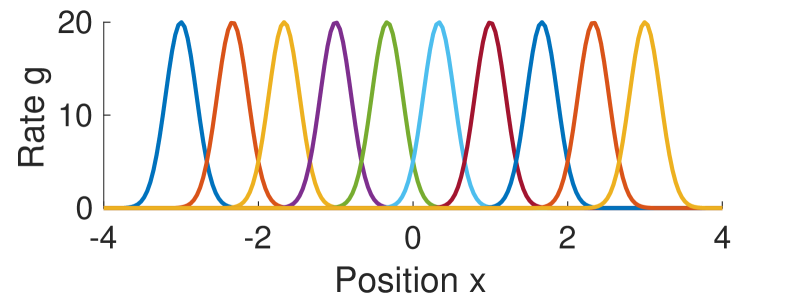
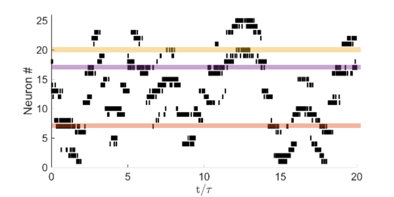
We first consider decoding from a one-dimensional toy model with $d=10$ model neurons. These neurons have equal place-field width and maximal firing rate $g_{0}$, and their place-field centers are distributed equally within a certain range on the $x$ axis. (Figure 1(a)).

In this example, we consider both a linear hidden dynamics, i.e. an Ornstein-Uhlenbeck (OU) process with time scale $\tau$:

$$dx_{t} = -\frac{1}{\tau}x_{t}\,dt+\sigma_{x}dw_{t},$$ (10)

which gives rise to a Gaussian stationary (prior) density with mean $\mu_{x,\infty}=0$ and variance $\sigma_{x,\infty}=\frac{1}{2}\sigma_{x}^{2}\tau$. As an alternative, we also consider a nonlinear hidden dynamics:

$$dx_{t} = \theta x_{t}(\gamma-x_{t}^{2})\,dt+\sigma_{x}dw_{t}.$$ (11)

The resulting stationary distribution is symmetric and bimodal, with two distinct modes at $x=\pm\gamma$.

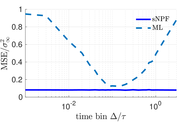
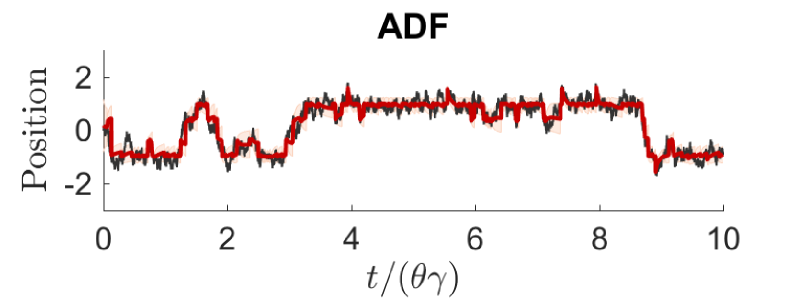
For the linear dynamics, we first compare the filtering performance of the sNPF in terms of its mean-squared error (MSE) to that of a simple maximum likelihood (ML) decoder (see Section S 2.1 for details). This decoder does not take into account any prior knowledge about the hidden process $\mathbf{x}_{t}$, and thus simply relies on the information given by the spikes trains. Further, its performance is heavily dependent on temporal binning of the spike train (Figure 1(b)), which makes it difficult to use practically. Certainly, the optimal bin size for decoding depends on the effective firing rate of the neurons as well as on the hidden dynamics, and is difficult to determine analytically. Using a filtering algorithm such as the sNPF instead has the advantage of being independent of hand-tuned temporal binning, and for the example simulation shown in Figure 1(b) yields a much better performance than the ML decoder.

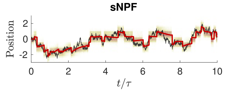
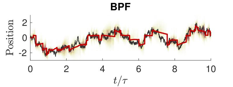
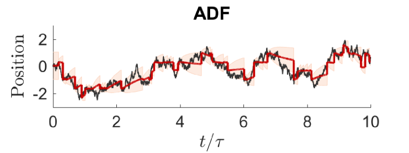
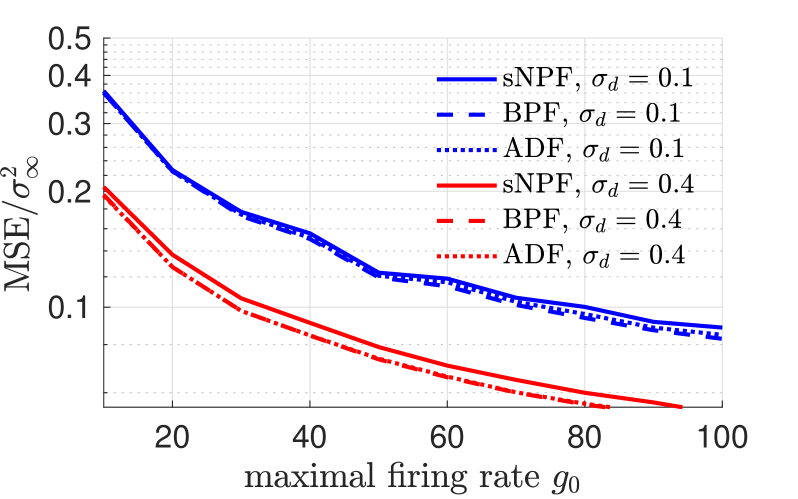
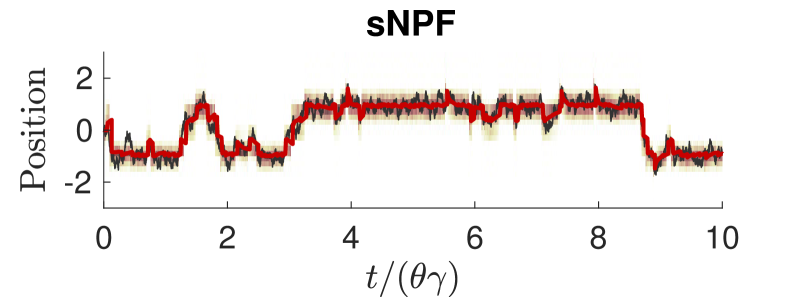
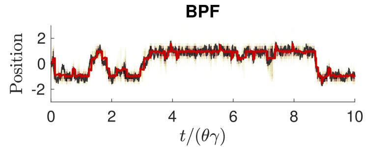
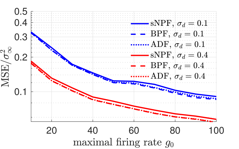
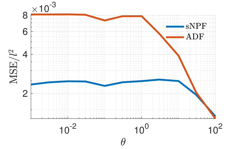
We further compared the sNPF to other filtering algorithms, i.e. the BPF and the ADF, which by definition do take into account prior knowledge in terms of the hidden dynamics given by Eq. (2). In Figure 1b and c, we show sample tracking simulations from these algorithms for both the linear and the nonlinear model, as well as a comparison of filtering performance. For the linear model, the performance of the ADF is indistinguishable from that of the BPF. This implies that the Gaussian approximation needed for the ADF to work is indeed justified for this particular model. Interestingly, the same applies for the nonlinear model, even though one would have expected the ADF to perform worse due to the nonlinearity. That its MSE is almost indistinguishable from that of the BPF demonstrates that for the parameters tested here, the Gaussian approximation is still valid. However, the picture changes slightly if the effective rate of point emission events is decreased, e.g. if there are only a few neurons with relatively low firing rate. Then, the posterior becomes bimodal, and multimodality cannot be captured by the assumed-density filter (ADF) that by construction relies on a unimodal approximation.

Even though the sNPF is a very heuristic approximation, and particle dynamics relies on the dynamics of only the first moment, the sNPF performs almost as good as the benchmark. What is notable, however, is that apparently higher-order moments fall short when compared to that of the benchmark filters, in particular in intermediate effective firing rate regimes (compare for instance the discussion on the second moment of the sNPF in Section S 3 of the SI).

(a)

(b)

(c) Linear hidden dynamics.

(d) Nonlinear hidden dynamics.

Figure 1: One-dimensional place-cell decoding. (a) Illustration of place fields. Here, $m=10$ neurons with place field centers $\mu_{d}$ spaced equally between -3 and 3, place field width $\sigma_{d}=0.2$ and maximal firing rate $g_{0}=20$. (b) Comparison of filtering performance of ML decoder versus sNPF as a function of time bin size $\Delta$. The hidden dynamics follows an OU process (Eq. 10) with $\tau=1$ and $\sigma_{x}=\sqrt{2}$. (c) Tracking simulation of the sNPF, BPF and ADF. The hidden dynamics is given by the black line (OU process) and the red line corresponds to the estimated first posterior moment of the corresponding filter. For the particle filters, shadings correspond to (weighted) particle density and thus estimated posterior density, with regions of high density appearing darker than regions of low density. For the ADF, the shaded regions denote the square root of the estimated posterior moment, i.e. $\sqrt{\Sigma_{t}}$. The lower panel shows the filtering performance in terms of MSE for different place field widths and maximal firing rates. The plots for BPF and ADF are almost indistinguishable by eye, and performance is only slightly better than the sNPF. (c) Same as (b), but with a nonlinear hidden dynamics (Eq. (11) with $\theta=-3$, $\gamma=1$ and $\sigma_{x}=\sqrt{2}$).

4.2 Restricted Brownian motion model

Let us now consider a more realistic toy example of an animal moving in a two-dimensional, confined box $\mathcal{D}$, with $d=25$ spatially-tuned neurons. Taking into account that animal movements are usually rather smooth, we model the movement within the box as an integrated Brownian motion, i.e. we augment the hidden space by a velocity component $\mathbf{v}_{t}$. Thus, the hidden dynamics are given by a reflected stochastic differential equation (RSDE, cf. [33]):

$$d\mathbf{x}_{t} = \mathbf{v}_{t}\,dt+\mathbf{k}_{t}\,dt,$$ (12)

$$d\mathbf{v}_{t} = -\beta(\mathbf{v}_{t}-\boldsymbol{\psi}(\mathbf{x}_{t}))\,dt+\Sigma_{v}^{1/2}d\mathbf{w}_{v,t},$$ (13)

resulting in the hidden state $[\mathbf{x}_{t},\mathbf{v}_{t}]^{T}\in\mathbb{R}^{4}$. Here, $\beta$ is a constant, $\mathbf{w}_{v,t}\in\mathbb{R}^{2}$ is a 2-dimensional Brownian-motion process and $\boldsymbol{\psi}(\mathbf{x}_{t})$ can be thought of as the negative gradient of a potential surface, e.g. $\boldsymbol{\psi}(\mathbf{x}_{t})=-\nabla_{\mathbf{x}}H(\mathbf{x}_{t})$. For simplicity, in our simulation we will use a linear function $\boldsymbol{\psi}=-\theta\mathbf{x}_{t}$, but in general we would assume that animal movement is governed by a much more complicated nonlinearity [17].

The process $\mathbf{k}_{t}$ is the minimal process needed to restrict the position $\mathbf{x}_{t}$ to lie within the box $\mathcal{D}$ [34]. A possible realization of the process $\mathbf{k}_{t}$ is [33]:

$$\mathbf{k}_{t} = \begin{cases}0&\text{if }\mathbf{x}_{t}\in\mathcal{D}\\ -\left(\mathbf{n}(\mathbf{x}_{t})^{T}\mathbf{v}_{t}\right)\mathbf{n}(\mathbf{x}_{t})&\text{if }\mathbf{x}_{t}\in\partial\mathcal{D}\end{cases},$$ (14)

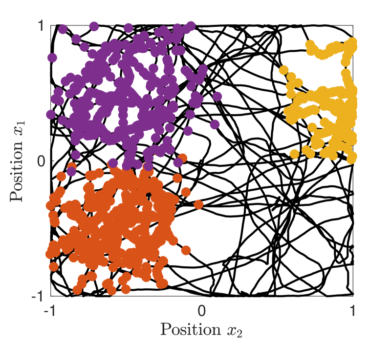
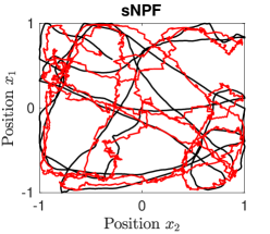
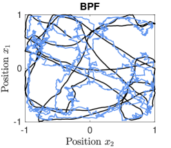
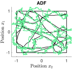
where $\mathbf{n}$ is a normal vector perpendicular to the boundary $\partial\mathcal{D}$. This process effectively cancels the velocity component perpendicular to the boundary and thus implements boundary conditions of the von Neumann type. A sample trajectory of the resulting process (with corresponding responses of spatially tuned neurons) is shown in Figure 2(a).

The boundary condition can be directly implemented in the sNPF and the BPF using a projection approach (cf. [34, 35, 33]). However, in the ADF, these cannot be directly implemented, because the process in Eq. (14) imposes a strong nonlinearity, such that the Gaussian approximation is violated at the boundaries. The only possibility is to avoid explicitly modeling the boundary process $\mathbf{k}_{t}$ in the ADF altogether, and rely on the filter estimate being ’driven back’ into the box $\mathcal{D}$ by the spiking events (Figure 2(b)).

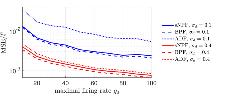
The numerical performance of the sNPF for this rather complex model is again strikingly close the the benchmark (BPF) for all parameters tested, as shown in Figure 2(d). On the other hand, the numerical performance of the ADF strongly depends on the particular choice of the parameters. More precisely, if the simulation setup is sufficient to keep the filter trajectory well within the boundaries (e.g. for large effective firing rates or for a strong drift towards the center modified by $\theta$, cf. Figure 2(e)), then the ADF performs reasonably well. If this is not the case, the numerical performance of the ADF is much worse than that of the sNPF.

(a)

(b)

(c)

(d)

(e)

Figure 2: Two-dimensional place-cell decoding in confined region. (a) Sample trajectory (spatial components) of hidden process in Eq. (12) and (13), and responses of 3 (out of $d=25$) spatially tuned sample neurons. Here, we use the model parameters $\beta=0.5$, $\theta=2$, $\Sigma_{v}=2\cdot\mathbb{I}^{2\times 2}$, $g_{0}=80$, $\Sigma_{d}^{1/2}=\sigma_{d}\cdot\mathbb{I}^{2\times 2}$ with $\sigma_{d}=0.2$, and the place field centers $\boldsymbol{\mu}_{d}$ are distributed on an equally-spaced grid in the spatial domain covering the whole box $\mathcal{D}$. The trajectory shown here was run for $T=100\cdot\theta^{-1}$. (b) Sample spike train corresponding to the first 20 time constants $\theta^{-1}$. (c) Decoding the spike train in (b) with the sNPF, BPF and the ADF. Note that the ADF trajectory may leave the box because reflecting boundary conditions cannot be incorporated. (d) Numerical filtering performance in terms of MSE for the three filtering algorithms, averaged over $T=1000\cdot\theta^{-1}$. (e) A large drift parameter $\theta$ is able to ‘pull’ the ADF estimate away from the boundaries, making it almost optimal again. Note that for this example exceptionally large values of $\theta$ are needed. Here, $\sigma_{d}=0.1$.

5 On the COD in weighted approaches

In contrast to standard particle filtering algorithms, such as the sequential importance sampling algorithm [20], the particles in Eq. (6) are considered equally weighted. This comes with what we consider a huge advantage: weighted particle filtering approaches are known to suffer from inevitable weight decay over time [36], an effect that becomes more severe as the dimensionality of the problem increases [25] (see also Section S 4.3 in the SI).

To illustrate the problem, consider the BPF [20], which represents the posterior with a weighted empirical distribution:

$$p(\mathbf{x}_{t}|\mathbf{N}_{0:t}) \approx \sum_{i=1}^{P}w_{t}^{(i)}\delta(\mathbf{x}_{t}-\mathbf{x}_{t}^{(i)}),$$ (15)

where the (normalized) importance weights $w_{t}^{(i)}$ change dynamically over time.

For continuous-time models, it is possible to write down an SDE that describes the dynamics of the weights (see Section S 4.2.1, Eq. S-43, in the SI). From this, we obtain an SDE for the inverse of the ‘number of effective particles’ $P_{\text{eff}}^{-1}=(\sum_{i}(w_{t}^{(i)})^{2})^{-1}$, which may be considered as an empirical estimate of how many particles are effectively representing the posterior. If all weights are equal, i.e. $w_{t}^{(i)}=1/P\ \forall i$, then $P_{\text{eff}}=P$. If, on the other hand, one weight is $1$ and all the other weights are zero, we find $P_{\text{eff}}=1$. In the latter case, the system is highly degenerate, and only a single particle contributes to representing the posterior. The SDE for $P_{\text{eff}}^{-1}$ reads (Eq. S-45 in the SI):

$$dP_{\text{eff}}^{-1} = \sum_{i,d=1}^{P,m}(w_{t}^{(i)})^{2}\left[-2(g_{d}(\mathbf{x}_{t}^{(i)})-\bar{g}_{d})\,dt+(g_{d}(\mathbf{x}_{t}^{(i)})^{2}-\bar{g}_{d}^{2})\frac{1}{\bar{g}_{d}^{2}}\,dN_{t}^{(d)}\right],$$ (16)

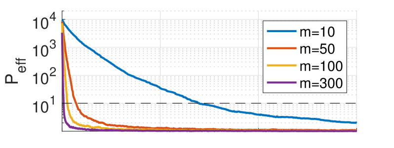
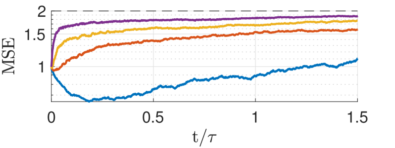
where the bar denotes an empirical estimate according to the particle distribution. In Figure 3(a), we perform simulations showing that the effective number of particles $P_{\text{eff}}$ decreases over time (Figure 3(a)). This is accompanied by an increase in MSE that tends towards $\text{MSE}=2$, corresponding to that of an independent draw from the hidden process, i.e. without any knowledge of the observations.

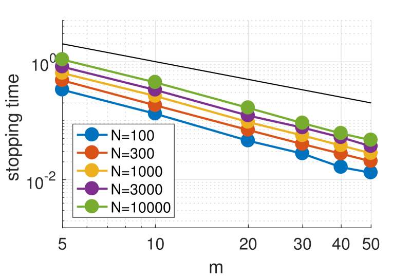
Let us now make this numerical observation of a dynamical weight degeneration more formal and consider initializing a system with equal weights and particle positions that are drawn from the true posterior. Similarly to the argument made in Surace et al. [25], this equation gives us an estimate of the initial rate of decay of the effective number of particles: since this equation has $m$ summands, a rough estimate of the decay time scale of $P_{\text{eff}}$ is $\tau_{decay}\propto\frac{1}{m}$ (please see Section S 4.3 in the SI for more details on this argument). Even more, the simulations in Figure 3(b) suggest that this analytical argument seems to even underestimate the rate on which the particles degenerate, as it seems to happen - at least numerically - on an even faster time scale.

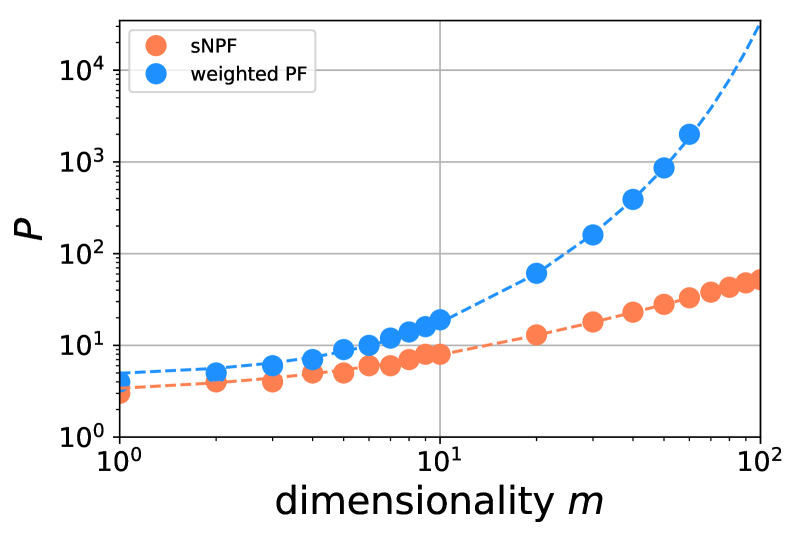
Thus, the higher the dimensionality of the system, or rather the dimensionality of the observed process, the more particles need to be in the system to compensate for the fast decay - even if numerical tricks such as particle resampling are applied. To demonstrate this, we performed simulations where we determined the minimum number of particles that are needed for a fixed numerical filtering performance of $0.8\%$ of the optimal MSE in a nonlinear model, both with the sNPF and with a standard BPF. The minimum number of particles needed for the BPF increases exponentially with problem dimensionality $m$, whereas the BPF only scales linearly with dimensions (Figure 3(c)).

In earlier work, Huang et al. [17] suggested particle filters as a possible alternative for decoding of nonlinear models, but also mention numerical issues found earlier [37]. Practically, our analysis aims to demonstrate that weighted PFs are not advantageous for decoding if the dimensionality of the observations, for instance the number of recording electrodes, is large. Thus, for these cases, unweighted particle filtering approaches offer a suitable alternative to weighted approaches.

(a)

(b)

(c)

Figure 3: The COD in weighted particle filters. (a) Importance weights of the BPF decay over time, illustrated by the depletion of the effective number of particles $P_{\text{eff}}$. At the same time, the MSE increases, indicating a significant drop in performance. Note that $\text{MSE}=2$ denotes a filtering performance that corresponds to taking a single sample from the hidden dynamics in Eq. (2), employing no knowledge of the observations. (b) Time to reach $P_{\text{eff}}=10$ (‘stopping time’) as a proxy for the particle decay time scale. The black line denotes a $1/m$ scaling. The time to reach $P_{\text{eff}}=10$ decreases faster upon increasing the problem dimensionality $m$. In (a) and (b), the model is a multidimensional Ornstein-Uhlenbeck (OU) process with exponential firing rate function. (c) The number of particles needed for a fixed performance (of $80\%$ of the optimal MSE) across dimensions scales exponentially in a BPF and linearly in the sNPF. In this simulation, a nonlinear hidden dynamics, $f(x)\propto x(x^{2}-1)$, with exponential firing rate function $g(x)\propto\exp\left(2x\right)$ was used.

6 Adaptive Encoding

In a broad sense, encoding aims to find the relationship between the hidden stimulus $\mathbf{x}_{t}$ and the neural spike train. Here, we narrow this task down to finding the parameters of a previously specified model. In this section, we use the particle filter ansatz outlined in the previous section to approximate an encoding scheme. The resulting algorithm is suitable for both offline and online (‘adaptive’) encoding when the hidden state cannot be directly observed, for instance when adjusting parameters in brain-machine interfaces [3, 4].

6.1 Maximum likelihood encoding

As an objective function for learning the model parameters in Eq. (1) and (2) we use the incomplete-data log likelihood, which is given by (see Section S 5.1 in SI):

$$\Lambda_{t}^{\theta} = \sum_{d=0}^{m}\left(\int_{0}^{t}\log\frac{\mathbb{E}\left[g_{d}(\mathbf{x}_{s})|\mathbf{N}_{0:s}\right]}{\lambda_{0}}dN_{d,s}+\int_{0}^{t}(\lambda_{0}-\mathbb{E}\left[g_{d}(\mathbf{x}_{s})|\mathbf{N}_{0:s}\right])\,ds\right),$$ (17)

where $\lambda_{0}$ is a constant reference firing rate, which is needed in the derivation and does not affect likelihood optimization. Since in a general task we do not have access to the posterior expectations, these are approximated with $\mathbb{E}\left[g_{d}(\mathbf{x}_{t})|\mathbf{N}_{0:t}\right]\approx\langle g_{d,t}\rangle$ from the sNPF particle estimates according to Eq. (8). From this perspective, the optimal set of parameters $\theta$ maximizes the log likelihood function for a given set of observations $\mathbf{N}_{0:t}$.

6.2 Learning rules

Update rules for the parameters $\theta$ can be obtained by performing a gradient ascent on Eq. (17), using sNPF approximations.

$$d\theta = \eta_{\theta}\,\partial_{\theta}\Lambda_{t}^{\theta}$$ (18)

$$\approx \eta_{\theta}\,\sum_{d=0}^{m}\int_{0}^{t}\left(\partial_{\theta}\langle g_{d,s}\rangle\right)\left(\frac{1}{\langle g_{d,s}\rangle}dN_{d,s}-ds\right)$$

$$= \eta_{\theta}\int_{0}^{t}\left(\partial_{\theta}\langle\mathbf{g}_{s}\rangle\right)^{T}\text{diag}(\langle\mathbf{g}_{s}\rangle)^{-1}\left(d\mathbf{N}_{s}-\langle\mathbf{g}_{s}\rangle ds\right)$$

where $\eta_{\theta}$ is a (possibly time-dependent) learning rate. Noting that $\langle\mathbf{g}_{t}\rangle$ can be considered a posterior estimate of the firing rate variance $\Sigma_{g,t}$, the learning rules read:

$$d\theta = \eta_{\theta}\int_{0}^{t}\left(\partial_{\theta}\langle\mathbf{g}_{s}\rangle\right)^{T}\Sigma_{g,t}^{-1}\left(d\mathbf{N}_{s}-\langle\mathbf{g}_{s}\rangle ds\right)$$ (19)

Online learning rules are obtained by maximizing the infinitesimal increments of the log likelihood in Eq. (17) at each point in time, while the sequence of observations $\mathbf{N}_{0:t}$ keeps flowing in. This can only be expected to converge if certain ergodicity requirements of the whole stochastic process are fulfilled (a proof for this, albeit for continuous-time observations, can be found in [38]). Assuming process ergodicity, the online learning rules read:

$$d\theta = \eta_{\theta}\left(\partial_{\theta}\langle\mathbf{g}_{t}\rangle\right)^{T}\Sigma_{g,t}^{-1}\left(d\mathbf{N}_{t}-\langle\mathbf{g}_{t}\rangle dt\right)$$ (20)

Note that for both the offline and online learning rules depend on the derivative of a posterior expectation, i.e. $\partial_{\theta}\langle\mathbf{g}_{t}\rangle$. When computing this derivative, we have to take into account the change of the rate function $\mathbf{g}$ as well as the infinitesimal changes in the filter with respect to the parameters $\theta$. The latter is referred to as ’filter derivative’ and in general cannot be computed in closed form. However, using the particle representation of the sNPF allows us to compute a filter derivative for every single particle and thus approximate Eq. (19) and (20). For details, see Section S 5.2 in the SI.

6.3 Learning the gain matrix $W_{t}$

As an alternative to using the EKSPF, we can determine the gain matrix by treating it as a parameter (‘decoding parameter’) that can be learned online. We can immediately write down the online learning rule for the components of the gain matrix, $W_{ij}$ using Eq. (20) and the fact that there is no explicit dependence of the functions $\mathbf{f}$ and $\mathbf{g}$ on $W$ (cf. Eq. S-50 in SI Section S 5.2):

$$dW_{ij} = \eta_{W_{ij}}\left(\langle D\mathbf{g}_{t}\cdot\boldsymbol{\alpha}_{W_{ij},t}\rangle\right)^{T}\Sigma_{g,t}^{-1}\left(d\mathbf{N}_{t}-\langle\mathbf{g}_{t}\rangle dt\right),$$ (21)

with filter derivative dynamics

$$d\boldsymbol{\alpha}_{W_{ij},t}^{(k)} = D\mathbf{f}_{t}^{(k)}\cdot\boldsymbol{\alpha}_{W_{ij},t}^{(k)}dt$$ (22)

$$+\left(d\mathbf{N}_{t}-\mathbf{g}_{t}^{(k)}\,dt\right)_{j}\mathbf{e}_{i}-W_{t}\cdot D\mathbf{g}_{t}^{(k)}\cdot\boldsymbol{\alpha}_{W_{ij},t}^{(k)}\,dt,$$

where $\mathbf{e}_{i}$ denotes the unit vector in $i$-direction, and $\left(D\mathbf{f}_{t}\right)_{i,j}=\partial_{x_{j}}f_{i}$ and $\left(D\mathbf{g}_{t}\right)_{i,j}=\partial_{x_{j}}g_{i}$ denotes the Jacobian of the functions $\mathbf{f}_{t}$ and $\mathbf{g}_{t}$, respectively.

Note that the resulting filtering scheme is based on the heuristic ansatz in Eq. (6) that is compensated for in a rigorous way by choosing the gain such that the incomplete-data log likelihood is maximized.

7 Discussion

In this paper, we proposed an ansatz for a recursive filtering algorithm for point-process observations, the spike-based Neural Particle Filter (sNPF). Since it relies on an approximation of the posterior density by equally weighted, empirical samples, it can be seen as an unweighted particle filtering method. One realization of this general ansatz uses an empirical approximation for the weight matrix that governs the strength of the particle updates due to the point-process observations, has been put forward before and is called ensemble Kushner-Stratonovich-Poisson filter (EKSPF,[32]). Despite its relevance for neuroscience and in particular decoding, this filter has not received much attention in the community yet. In addition, a thorough analysis of its capabilities is hitherto lacking. Here, we showed that its decoding performance in a toy decoding task, which was motivated by a realistic problem setting, is almost optimal, and even may outperform an ADF due of its flexibility. Further, we demonstrated its usefulness for higher dimensional models, which become essential in times when growingly sophisticated probes allow for an ever increasing amount of simultaneously recorded neurons. In particular, we showed that it is a promising candidate for a filtering algorithm that avoids the COD, in contrast to standard PFs. Lastly, the sNPF can be used to approximate a likelihood function, that allows the derivation of both online and offline learning rules for system identification.

The idea to frame the decoding task as a question of Bayesian inference is certainly not a new one and has been around ever since the discovery that neuronal spiking can be, to some extent, modeled by a Poisson process. For static stimuli, maximum a-posteriori (MAP) methods have proven successful, in particular for generalized linear models where the (complete-data) likelihood function is convex [13, 12]. A straightforward extension to dynamic stimuli can be obtained by considering averaging spikes over a fixed time window [8, 13]. A similar problem as with ML decoding arises here as well (Figure 1(b)): the decoding accuracy in a dynamic setting will crucially depend on how large the time window is chosen. Further, MAP estimates tend to exhibit a large decoding error whenever the posterior density deviates significantly from a unimodal density [24].

Alternatively, variational inference (cf. [39]) aims at matching the posterior and a (usually Gaussian) proposal by minimizing the Kullback-Leibler divergence between the two densities with respect to the proposal parameters. For specific models with point-process observations, the parameters can be solved for in closed form [12], but it is unclear how this result would relate to other models, e.g. Gaussian-shaped tuning curves. Further, the discussion in [12] is restricted to a static setting, and it would be interesting to see whether it can be extended to a dynamical setting, which has been done for instance for continuous-time observations [40].

An important class of models used for decoding are (Gaussian) assumed density filters (ADF), which are particularly suited to decode from Gaussian-shaped tuning curves. ADFs are available for both discrete [7, 26] and continuous time [41, 31] models. The Gaussian approximation in the filters by Brown, Eden and coworkers result from a second-order Taylor expansion of the posterior density, and is thus roughly along the lines of an extended Kalman filter (EKF) for continuous-time observations. As a second example, the ADF in [31] directly approximate posterior estimates in the filtering equations for mean and variance under the Gaussian assumption. In this regard, it is surprising that, even if the hidden dynamics is nonlinear (cf. Section 4.1), the ADF exhibits almost optimal performance - as long as the posterior is still sufficiently Gaussian-shaped. For our simulations, we chose the ADF by Harel et al. [31] as a comparison, because the mindset in the heuristic derivation of the sNPF is similarly circular: assuming the posterior to be approximated by $\delta$-masses, we approximate any posterior estimates that appear in the dynamical equations of the particles by estimates under this empirical density.

Both ADF versions suffer from the fact that they have to be computed explicitly for each particular model, which can turn out to be tedious or even impossible analytically. Thus, they are also very limited in their model flexibility: as long as the decoding task is comparatively simple with sufficiently linear hidden dynamics and exponential rate function, this class of filters offers a suitable and computationally efficient decoding scheme. However, more complex tasks, for instance when introducing boundary conditions like in in Section 4.2, first might imply a serious violation of the Gaussian assumption at the boundaries and, second, might lead to a significant drop in performance of the ADF when neglected. For these ‘complex’ tasks, the sNPF turns out to be superior, because it can accommodate a huge variety of generative models, linear and nonlinear. Due to the specific representation scheme, it is possible to represent multimodal posterior densities. Further, the implementation does not require computing any further instances of the model, such as posterior expectations or derivatives, but just needs being able to evaluate the hidden function $\mathbf{f}$ and the rate function $\mathbf{g}$ at the particle positions.

Since it approximates the posterior density with empirical samples, the sNPF can be seen as a PF, albeit without importance weights. Standard weighted PFs are still considered state-of-the-art filtering algorithms, because they are asymptotically exact in the limit of infinite particles, can be derived rigorously from a change of measure approach (cf. Section S 4 in the SI) and, last but not least, are easily implementable numerically. Because they are not limited in their flexibility, particle-based methods may enhance decoding performance by tackling multi-modality [24] and/or model nonlinearities [17]. Unfortunately, it is known (cf. also Section 5) that they suffer from an inevitable weight decay over time, leading to a decline in the number of particles that effectively represent the posterior density.

The time scale on which weight decay occurs decreases with the number of observable dimension, effectively leading to a COD, as shown in Section 5. In continuous-time models, it might help to choose better proposal densities, which already take into account the observations in the proposal and then propagate the particles into significant regions in space. Finding such a proposal for point process observations is an open problem even in discrete time, as for instance the ‘optimal proposal’ [20] can be computed only for very specific models. Further, resampling the particles frequently is known to numerically boost the BPF performance. However, since the time scale on which resampling is beneficial is independent of the problem dimensionality (cf. [25]), resampling is not a sufficient technique to avoid the COD. Another remedy could be to use an ADF as proposal density for the particles [37], but it is has not been studied yet whether this approach can avoid or mitigate the COD. Unweighted PF approaches, such as the Neural Particle filter (NPF, [30] or the Feedback Particle filter (FBPF, [42]), hold the promise of avoiding the COD (Figure 3, cf. also [25]), because they trivially do not suffer from weight decay. The derivation of the sNPF relies on a heuristic similar to related equally-weighted particle filtering approaches for continuous-time observations (e.g. [30]), and as such it is not surprising that similar properties emerge.

Here, we have used the sNPF to approximate the incomplete-data log likelihood, i.e. the likelihood function of the spike train without knowledge of the hidden state. The resulting learning rules can thus be used for an unsupervised learning task, which has not received much attention in neuroscience yet. Usually, encoding is done in a supervised way, because one has access to the ground truth. One of the few examples of parameter learning, that is both online and unsupervised, was tackled in [26] by state augmentation: imposing a linear dynamics on the parameters, the same algorithm is applied for the learning task as for the decoding task. In general, it is not clear whether this algorithm maximizes the log likelihood of the whole observation sequence, in particular when the filtering algorithm is approximate. For learning with the sNPF, a similar question arises: how can we be sure that learning is accurate if the filter is approximate? Fortunately, it can be shown (for continuous-time models) that parameter learning based on maximum likelihood can make up for an approximate filter, such that estimated state and estimated parameters together maximize the incomplete-data log likelihood [38]. Offline learning can in principle be tackled with huge flexibility by expectation maximization (EM, [43]) combined with particle smoothing [44], which can be computationally expensive. Alternatively, for models where it is applicable if applicable, a Gaussian approximation leads to closed-form EM update equations [12].

A serious limitation of the sNPF is that it apparently does not capture the full posterior density. By construction, the particle dynamics are such that the dynamics of the first posterior moment matches that from the first moment of the particle density, under the assumption that higher-order moments in this particle dynamics are matched (in the case of the EKSPF). It is surprising that, despite this assumption to be violated (similarly to an ADF), it does not seem to significantly affect state estimation as measured by MSE. However, already the variance estimated from the particle distribution deviates to a large extent from that estimated by a BPF. Analytically, we find that it does not take into account the instantaneous reduction in variance following an event. Further, the variance in generally evolves slower than that of the benchmark. To tackle this particular problem, one would need to tune the whole ansatz (not just the gain matrix), for instance by choosing a different noise covariance, such that, at least in between events, the variance can be matched. In this regard, a thorough error analysis for the EKSPF, which is hitherto lacking, might help to choose the model accordingly, if one is interested in accurately determining higher-order posterior moments. In general, it would be desirable to ultimately derive an unweighted particle filter that is asymptotically exact, such as the FBPF [42] for continuous-time observations.

Despite its limitations, the sNPF is a decoding algorithm that is suitable for spike-train decoding. In particular, it becomes an interesting alternative to an ADF for complex models, which exhibit strong nonlinearities, boundary conditions, or cannot be computed with an ADF in closed form. For high-dimensional models, since it does not suffer from the COD, it outperforms a BPF for a limited number of particles. Thus, the sNPF might prove beneficial when compared to standard approaches as more and more neurons can be simultaneously recorded. Lastly, it might motivate related, similarly scalable algorithms, that will become crucial in the future of neuroscience.

References

- [1] Stevenson IH, Körding KP. How advances in neural recording affect data analysis. Nature Neuroscience. 2011;14(2):139–142. Available from: http://dx.doi.org/10.1038/nn.2731.
- [2] Jun JJ, Steinmetz NA, Siegle JH, Denman DJ, Bauza M, Barbarits B, et al. Fully Integrated Silicon Probes for High-Density Recording of Neural Activity. Nature. 2017;in press(7679):232–236. Available from: http://dx.doi.org/10.1038/nature24636.
- [3] Donoghue JP. Connecting cortex to machines: Recent advances in brain interfaces. Nature Neuroscience. 2002;5(11s):1085–1088.
- [4] Shanechi MM, Orsborn AL, Carmena JM. Robust Brain-Machine Interface Design Using Optimal Feedback Control Modeling and Adaptive Point Process Filtering. PLoS Computational Biology. 2016;12(4).
- [5] Bremaud P. Point Processes and Queues: Martingale Dynamics. Springer Series in Statistics. Springer New York; 1981. Available from: https://books.google.ch/books?id=k5jarX-BssUC.
- [6] Davidson TJ, Kloosterman F, Wilson MA. Hippocampal Replay of Extended Experience. Neuron. 2009;63(4):497–507. Available from: http://dx.doi.org/10.1016/j.neuron.2009.07.027.
- [7] Brown EN, Frank LM, Tang D, Quirk MC, Wilson Ma. A statistical paradigm for neural spike train decoding applied to position prediction from ensemble firing patterns of rat hippocampal place cells. Journal of Neuroscience. 1998;18(18):7411–25. Available from: http://neuro.cjb.net/cgi/content/abstract/18/18/7411.
- [8] Zhang K, Ginzburg I, McNaughton BL, Sejnowski TJ. Interpreting neuronal population activity by reconstruction: unified framework with application to hippocampal place cells. Journal of Neurophysiology. 1998 feb;79(2):1017–44. Available from: http://www.ncbi.nlm.nih.gov/pubmed/9463459.
- [9] Barbieri R, Frank LM, Nguyen DP, Quirk MC, Solo V, Wilson MA, et al. A Bayesian decoding algorithm for analysis of information encoding in neural ensembles. The 26th Annual International Conference of the IEEE Engineering in Medicine and Biology Society. 2004;4:4483–4486. Available from: http://ieeexplore.ieee.org/document/1404246/.
- [10] Truccolo W. A Point Process Framework for Relating Neural Spiking Activity to Spiking History, Neural Ensemble, and Extrinsic Covariate Effects. Journal of Neurophysiology. 2004;93(2):1074–1089. Available from: http://jn.physiology.org/cgi/doi/10.1152/jn.00697.2004.
- [11] Koyama S, Eden UT, Brown EN, Kass RE. Bayesian decoding of neural spike trains. Annals of the Institute of Statistical Mathematics. 2010;62(1):37–59.
- [12] Macke JH, Buesing L, Sahani M. Estimating state and parameters in state space models of spike trains. In: Chen Z, editor. Advanced State Space Methods for Neural and Clinical Data. Cambridge: Cambridge University Press; 2011. p. 137–159. Available from: http://ebooks.cambridge.org/ref/id/CBO9781139941433A054.
- [13] Pillow JW, Ahmadian Y, Paninski L. Model-Based Decoding, Information Estimation, and Change-Point Detection Techniques for Multineuron Spike Trains. Neural Computation. 2011;23(1):1–45. Available from: http://www.mitpressjournals.org/doi/10.1162/NECO{_}a{_}00058.
- [14] Snyder DL. Filtering and Detection for Doubly Stochastic Poisson Processes. IEEE Transactions on Information Theory. 1972;18(1):91–102.
- [15] Eden UT. Point Process Adaptive Filters for Neural Data Analysis: Theory and Applications. Decision and Control, 2007 46th IEEE Conference on. 2007;p. 5818–25. Available from: http://ieeexplore.ieee.org/lpdocs/epic03/wrapper.htm?arnumber=4434708.
- [16] Harel Y, Meir R, Opper M. A Tractable Approximation to Optimal Point Process Filtering : Application to Neural Encoding. Advances in Neural Information Processing Systems. 2015;p. 1–9. Available from: https://papers.nips.cc/paper/5863-a-tractable-approximation-to-optimal-point-process-filtering-application-to-neural-encoding.pdf.
- [17] Huang Y, Brandon MP, Griffin AL, Hasselmo ME, Eden UT. Decoding Movement Trajectories Through a T-Maze Using Point Process Filters Applied to Place Field Data from Rat Hippocampal Region CA1. Neural Computation. 2009;21(12):3305–3334. Available from: http://www.mitpressjournals.org/doi/10.1162/neco.2009.10-08-893.
- [18] Bobrowski O, Meir R, Eldar Y. Bayesian filtering in spiking neural networks: Noise, adaptation, and multisensory integration. Neural computation. 2009;p. 1–39. Available from: http://www.mitpressjournals.org/doi/abs/10.1162/neco.2008.01-08-692.
- [19] Legenstein R, Maass W. Ensembles of Spiking Neurons with Noise Support Optimal Probabilistic Inference in a Dynamically Changing Environment. PLoS Computational Biology. 2014 oct;10(10):e1003859. Available from: http://www.ncbi.nlm.nih.gov/pubmed/25340749.
- [20] Doucet A, Godsill S, Andrieu C. On sequential Monte Carlo sampling methods for Bayesian filtering. Statistics and Computing. 2000;10(3):197–208.
- [21] Kalman RE. A New Approach to Linear Filtering and Prediction Problems. Transactions of the ASME Journal of Basic Engineering. 1960;82(Series D):35–45. Available from: http://fluidsengineering.asmedigitalcollection.asme.org/article.aspx?articleid=1430402.
- [22] Kalman RE, Bucy RS. New Results in Linear Filtering and Prediction Theory. Journal of Basic Engineering. 1961;83(1):95. Available from: http://fluidsengineering.asmedigitalcollection.asme.org/article.aspx?articleid=1430804.
- [23] Brockwell AE. Recursive Bayesian Decoding of Motor Cortical Signals by Particle Filtering. Journal of Neurophysiology. 2004;91(4):1899–1907. Available from: http://jn.physiology.org/cgi/doi/10.1152/jn.00438.2003.
- [24] Ahmadian Y, Pillow JW, Paninski L. Efficient Markov Chain Monte Carlo Methods for Decoding Neural Spike Trains. Neural Computation. 2011;23(1):46–96. Available from: http://www.mitpressjournals.org/doi/10.1162/NECO{_}a{_}00059.
- [25] Surace SC, Kutschireiter A, Pfister JP. How to avoid the curse of dimensionality: scalability of particle filters with and without importance weights. 2017;(2002):1–16. Available from: http://arxiv.org/abs/1703.07879.
- [26] Eden UT, Frank LM, Barbieri R, Solo V, Brown EN. Dynamic analysis of neural encoding by point process adaptive filtering. Neural Computation. 2004 may;16(5):971–998. Available from: http://www.ncbi.nlm.nih.gov/pubmed/15070506.
- [27] Fairhall AL, Lewen GD, Bialek W, de Ruyter van Steveninck RR. Efficiency and ambiguity in an adaptive neural code. Nature. 2001 aug;412(6849):787–792. Available from: http://dx.doi.org/10.1038/35090500http://www.nature.com/doifinder/10.1038/35090500.
- [28] Frank LM, Brown EN, Stanley GB. Hippocampal and Cortical Place Cell Plasticity : Implications for Episodic Memory. Hippocampus. 2006;16:775–784.
- [29] Schoenenberger P, O’Neill J, Csicsvari J. Activity-dependent plasticity of hippocampal place maps. Nature Communications. 2016 jun;7(May):11824. Available from: http://www.nature.com/doifinder/10.1038/ncomms11824.
- [30] Kutschireiter A, Surace SC, Sprekeler H, Pfister Jp. Nonlinear Bayesian filtering and learning: a neuronal dynamics for perception. Scientific Reports. 2017 dec;7(1):8722. Available from: http://www.nature.com/articles/s41598-017-06519-y.
- [31] Harel Y, Meir R, Opper M. Optimal Encoding and Decoding for Point Process Observations: an Approximate Closed-Form Filter. ArXiv. 2016;p. 1–27. Available from: http://arxiv.org/abs/1609.03519.
- [32] Venugopal M, Vasu RM, Roy D. An Ensemble Kushner-Stratonovich-Poisson Filter for Recursive Estimation in Nonlinear Dynamical Systems. IEEE Transactions on Automatic Control. 2016 mar;61(3):823–828. Available from: http://ieeexplore.ieee.org/lpdocs/epic03/wrapper.htm?arnumber=7137635http://ieeexplore.ieee.org/document/7137635/.
- [33] Hanks EM, Johnson DS, Hooten MB. Reflected Stochastic Differential Equation Models for Constrained Animal Movement. Journal of Agricultural, Biological, and Environmental Statistics. 2017;22(3):353–372.
- [34] Lépingle D. Euler scheme for reflected stochastic differential equations. Mathematics and Computers in Simulation. 1995;38(1-3):119–126.
- [35] Dangerfield CE, Kay D, Burrage K. Modeling ion channel dynamics through reflected stochastic differential equations. Physical Review E. 2012;051907:1–15.
- [36] Daum F, Huang J. Curse of Dimensionality and Particle Filters. Proceedings of the IEEE Aerospace Conference. 2003;4:1979–1993.
- [37] Ergun A, Barbieri R, Eden UT, Wilson MA, Brown EN. Construction of Point Process Adaptive Filter Algorithms for Neural Systems Using Sequential Monte Carlo Methods. IEEE Transactions on Biomedical Engineering. 2007;54(3):419–428. Available from: http://ieeexplore.ieee.org/lpdocs/epic03/wrapper.htm?arnumber=4100829.
- [38] Surace SC, Pfister JP. Online Maximum Likelihood Estimation of the Parameters of Partially Observed Diffusion Processes. Arxiv. 2016;XX(3):1–10. Available from: http://arxiv.org/abs/1611.00170.
- [39] Opper M, Archambeau C. The Variational Gaussian Approximation Revisited. Neural Computation. 2009;21(3):786–792. Available from: http://www.mitpressjournals.org/doi/10.1162/neco.2008.08-07-592.
- [40] Archambeau C, Opper M, Shen Y, Cornford D, Shawe-Taylor J. Variational inference for diffusion processes. Advances in Neural Information Processing Systems. 2008;p. 1–8. Available from: http://books.nips.cc/nips20.html.
- [41] Eden UT, Brown EN. Continuous-time filters for state estimation from point-process models of neural data. Statistica Sinica. 2008 feb;18(4):1293–1310. Available from: http://www.nature.com/doifinder/10.1038/nrm2621http://www.ncbi.nlm.nih.gov/pubmed/22065511http://www.pubmedcentral.nih.gov/articlerender.fcgi?artid=PMC3208353http://www.nature.com/articles/nrm2621.
- [42] Yang T, Mehta PG, Meyn SP. Feedback particle filter. IEEE Transactions on Automatic Control. 2013;58(10):2465–2480.
- [43] Dempster AP, Laird NM, Rubin DB. Maximum likelihood from incomplete data via the EM algorithm. Journal of the Royal Statistical Society Series B Methodological. 1977;39(1):1–38. Available from: http://www.jstor.org/stable/10.2307/2984875.
- [44] Kantas N, Doucet A, Singh SS, Maciejowski J, Chopin N. On Particle Methods for Parameter Estimation in State-Space Models. Statistical Science. 2015 aug;30(3):328–351. Available from: http://projecteuclid.org/euclid.ss/1439220716.