Non-singular metric for an electrically charged point-source in ghost-free infinite derivative gravity

Abstract

In this paper we will construct a linearized metric solution for an electrically charged system in a ghost-free infinite derivative theory of gravity which is valid in the entire region of spacetime. We will show that the gravitational potential for a point-charge with mass $m$ is non-singular, the Kretschmann scalar is finite, and the metric approaches conformal-flatness in the ultraviolet regime where the non-local gravitational interaction becomes important. We will show that the metric potentials are bounded below one as long as two conditions involving the mass and the electric charge are satisfied. Furthermore, we will argue that the cosmic censorship conjecture is not required in this case. Unlike in the case of Reissner-Nordström in general relativity, where $|Q|\leq m/M_{p}$ has to be always satisfied, in ghost-free infinite derivative gravity $|Q|>m/M_{p}$ is also allowed, such as for an electron.

I Introduction

Einstein’s theory of general relativity (GR) has been tested to a very high precision in the infrared (IR) regime, i.e. at large distances and late times -C.-M. ; including the recent detections of gravitational waves due to merging of binaries which matches excellently the predictions of GR -B.-P. . However, as soon as one approaches short distances, the theory shows several problems, as for example black-hole and cosmological singularities at the classical level, and fails to be perturbatively renormalizable at the quantum level. Indeed, GR turns out to be incomplete in the ultraviolet (UV) regime, i.e. at short distances and small time scales.

It is well known that by adding quadratic terms in the curvature to the Einstein-Hilbert action one obtains a gravitational theory which becomes power counting renormalizable -K.-S. . In the UV, the theory becomes conformal and in the infrared Einstein’s GR is recovered, except that being a higher derivative theory of gravity, it suffers from instability due to the presence of a massive spin-$2$ ghost-like degree of freedom in the physical spectrum, whose emergence becomes evident by computing the graviton propagator around the Minkowski background -K.-S. .

Recently, it has been shown that the infinite derivative gravity (IDG) can resolve this ghost problem and, at the same time, it can also resolve the short-distance singularity for a point-like object, regularizing the $1/r$ behavior of the metric potential in the linearized limit, therefore ameliorating the UV aspects of Einstein’s and Newtonian gravity Biswas:2005qr ; Biswas:2011ar  . Furthermore, the time-dependent case yields a vacuum solution which is devoid of any cosmological singularity Biswas:2005qr ; Koivisto ; Koshelev:2012qn . It was also shown that the theory has a mass-gap at the linear level Frolov , and never develops a singularity even in a dynamical setup Frolov:2015bia ; Frolov:2015usa . At the linearized level, the non-trivial gravitational solution, in the UV, gives rise to constant Ricci scalar, Ricci tensor and Riemann tensor, and the Weyl tensor approaches zero at the origin (quadratically in distance from $r=0$ at best). The Kretschmann scalar remains constant and never blows up at the origin Buoninfante:2018xiw . Also, the static solution has now been extended to a non-singular rotating metric which resolves the Kerr-type ring singularity in Einstein’s GR Cornell:2017irh . In Ref. Boos:2018bxf , then authors have studied gravitational potentials in extended objects within ghost-free IDG, and found to be free from singularity.

Very recently, it has been shown that the full non-linear equations of motion for a ghost-free infinite derivative gravity, given by Biswas:2013cha , does not provide a $1/r^{\alpha}$, with $\alpha>0$, as a full vacuum solution Koshelev:2018hpt , where the Weyl term played the crucial role. Furthermore, in the time dependent context the infinite derivative gravity does not give rise to the Kasner-type metrics as vacuum solutions, and therefore provides a way to avoid the BKL-singularity which describes an anisotropic collapse of a time dependent metric solution in the case of the Einstein-Hilbert action Koshelev:2018rau .

As pointed out in Ref. conformal , the usual notion of vacuum solution that we use in GR, for example for the Schwarzschild solution, does not apply to the case of infinite derivative gravity. Indeed, the delta source distribution at $r=0$, which is imposed as a boundary condition, is smeared out by the infinitely many derivatives, generating an extended source whose size is given by the scale of non-locality, $r_{NL}\sim 2/M_{s}$ Koshelev:2017bxd . This point is crucial in order to obtain a full metric solution which is regular at $r=0.$

Infinite derivative gravity has also been discussed in the context of field theory. It is expected that infinite derivatives will ameliorate the quantum aspects as well, and it has been argued that such a class of theory will be super-renormalizable, see -Yu.-V. ; Tomboulis ; Talaganis:2014ida . Moreover, high energy scattering of gravitons in this class of theory does not necessarily lead to a formation of a blackhole as shown in Ref. Talaganis-scat . The scattering amplitude decreases exponentially, if the propagator and vertex corrections are correctly taken into account Talaganis:2014ida ; Talaganis-scat . Furthermore, in quantum field theory, infinite derivatives can be useful to understand the UV completion of the Standard Model Biswas:2014yia , and also the stability of the Higgs within the Abelian-Higgs model Ghoshal:2017egr .

Inspite of all these interesting results, there are many important challenges and unanswered riddles regarding IDG and the non-local regime of gravity, such as renormalizability, concept of spacetime, unitarity, causality structure, etc., indeed some of these issues have been discussed partly in Refs. Woodard ; Deser:2007jk ; Frolov:2017rjz ; Chin:2018puw ; Buoninfante:2018mre , but a clear quantum picture would be more desirable, and goes beyond the scope of the current paper. Among other things, the formulation of the initial value problem within the context of infinite-derivatives theories remains an interesting point of discussion Barnaby:2007ve .

The aim of this paper is to show how infinite derivative gravity will modify the gravitational potential generated by a charged source; we will produce a non-singular generalization of the Reissner-Nordström metric. We will briefly review the infinite derivative ghost-free gravity, then we will discuss the linearized metric of an electrically charged source. We will study various spacetime properties and discuss the consequences for the cosmic censorship hypothesis penrose ; hawking ; wald .

II Infinite derivative ghost-free gravity

The most general quadratic curvature gravity in $4$ dimensions, which is parity invariant and torsion free around a constant curvature background can be written as Biswas:2011ar ; Biswas:2016etb

$$\begin{array}[]{rl}S=&\displaystyle\frac{1}{16\pi G}\displaystyle\int d^{4}x\sqrt{-g}\left[{\mathcal{R}}+\alpha\left(\mathcal{R}\mathcal{F}_{1}(\Box_{s})\mathcal{R}\right.\right.\\ &\displaystyle\left.\left.+\mathcal{R}_{\mu\nu}\mathcal{F}_{2}(\Box_{s})\mathcal{R}^{\mu\nu}+\mathcal{R}_{\mu\nu\rho\sigma}\mathcal{F}_{3}(\Box_{s})\mathcal{R}^{\mu\nu\rho\sigma}\right)\right],\end{array}$$ (1)

where $G=1/M_{p}^{2}$ is Newton’s constant and $\alpha\sim 1/M_{s}^{2}$ is a dimensionful coupling. We are working with mostly positive metric signature $(-,+,+,+)$, and $\Box_{s}\equiv\Box/M_{s}^{2}$, where the d’Alembertian is given by: $\Box=g^{\mu\nu}\nabla_{\mu}\nabla_{\nu}$, and $\mu,\nu=0,1,2,3$. The new scale of gravity is given by $M_{s}\leq M_{p}$  . The three gravitational form factors ${\cal F}_{i}$ are reminiscent of any massless theory, and are constrained by the tree-level unitarity and ghost-free condition derived in Ref. Biswas:2011ar . Around the Minkowski background we can avoid the presence of other dynamical degrees of freedom other than the spin-$2$ massless graviton by first demanding

$$2{\cal F}_{1}(\Box_{s})+{\cal F}_{2}(\Box_{s})+2{\cal F}_{3}(\Box_{s})=0\,.$$ (2)

Thus, the propagator of this theory is given by Biswas:2011ar ; Biswas:2013kla ; Buoninfante

$$\Pi(-k^{2})=\frac{1}{a(-k^{2})}\left(\frac{\mathcal{P}^{(2)}}{k^{2}}-\frac{\mathcal{P}_{s}^{(0)}}{2k^{2}}\right)\,,$$ (3)

where $\Pi_{GR}=\mathcal{P}^{(2)}/k^{2}-\mathcal{P}_{s}^{(0)}/2k^{2}$ is the graviton GR propagator and $\mathcal{P}^{2},$ $\mathcal{P}_{s}^{0}$ are the two spin projection operators along the spin-$2$ and spin-$0$ components, respectively; while

$$a(\Box_{s})=1-\frac{1}{2}{\cal F}_{2}(\Box_{s})\Box_{s}-2{\cal F}_{3}(\Box_{s})\Box_{s}.$$ (4)

Moreover, in order to have no ghost-like degree of freedom, the form of $a(\Box)$ is restricted to be exponential of an entire function, so that no new poles are introduced in the propagator in Eq. (3). One simple choice is indeed

$$a(\Box_{s})=e^{-\Box/M_{s}^{2}}\,.$$ (5)

Other choices of entire function have been explored in Refs. Edholm:2016hbt , which illustrates universal behavior in the Newtonian potential from IR all the way up to the UV regime.

In Ref. Biswas:2011ar it was shown that the ghost-free condition, like in Eq. (5), also yields regular static solutions in the linear regime, where the metric potential satisfies: $2|\Phi|<1.$ Furthermore, in Ref. conformal , it was argued that this inequality can always hold true when the quadratic part of the action in Eq. (1) dominates over the Einstein-Hilbert term at the horizon scales . In this paper we will show that a similar scenario also holds when we consider the spacetime metric for a charged point-source, but in this case an additional inequality, involving the electric charge, will be required in order to have bounded metric potentials.

III Linearized metric solution for an electrically charged source

We now want to determine the spacetime metric for an electrically charged source in infinite derivative gravity, in the linear regime. The linearized field equations corresponding to the action in Eq. (1), with the ghost-free choice in Eq. (5) are given by Biswas:2011ar :

$$\begin{array}[]{ll}\displaystyle e^{-\Box/M_{s}^{2}}\left[\Box h_{\mu\nu}+(\eta_{\mu\nu}\partial_{\rho}\partial_{\sigma}h^{\rho\sigma}+\partial_{\mu}\partial_{\nu}h)\right.&\\ \,\,\,\,\,\,\,\,\,\,\,\displaystyle\left.-\partial_{\sigma}(\partial_{\nu}h^{\sigma}_{\mu}+\partial_{\mu}h_{\nu}^{\sigma})-\eta_{\mu\nu}\Box h\right]=-16\pi G\tau_{\mu\nu}.&\end{array}$$ (6)

The two-rank tensor $\tau_{\mu\nu}$ stands for the electro-magnetic energy-momentum tensor which is defined by:

$$\tau_{\mu\nu}=\frac{1}{4\pi}\left(\eta_{\rho\nu}F_{\mu\sigma}F^{\rho\sigma}-\frac{1}{4}\eta_{\mu\nu}F_{\rho\sigma}F^{\rho\sigma}\right),$$ (7)

where $F_{\mu\nu}=\partial_{\mu}A_{\nu}-\partial_{\nu}A_{\mu}$ is the electro-magnetic field strength, with $A_{\mu}$ being the potential-vector. We will consider the case in which the source is static and spherically symmetric, and no magnetic monopole is present, thus the only non-vanishing contributions of the electromagnetic field-strength will come from:

$$F_{10}=-F_{01}=E_{r}\quad\text{and}\quad E_{r}=\frac{Q}{r^{2}},$$ (8)

where $E_{r}$ is the radial component of the electric field, with the Coulomb constant $k_{e}=1$ in natural (Gaussian) units. We will work in the case of weak gravitational field and static source, so that the metric solution can be written as:

$$ds^{2}=-(1+2\Phi(r))dt^{2}+(1-2\Psi(r))(dr^{2}+r^{2}d\Omega^{2}),$$ (9)

where $(t,r,\theta,\varphi)$ are the isotropic coordinates, $d\Omega^{2}=d\theta^{2}+{\rm sin}^{2}\theta d\varphi^{2},$ and $\Phi$ and $\Psi$ are the two unknown gravitational fields that need to be found. By looking at the $00$-component and trace of the linearized field equations in Eq. (6) we obtain, respectively:

$$\begin{array}[]{rl}\displaystyle e^{-\nabla^{2}/M_{s}^{2}}\left[\nabla^{2}h_{00}-\partial_{i}\partial_{j}h^{ij}+\nabla^{2}h\right]=&-16\pi G\tau_{00},\\ \displaystyle e^{-\nabla^{2}/M_{s}^{2}}\left[-2\nabla^{2}h+2\partial_{i}\partial_{j}h^{ij}\right]=&-16\pi G\tau.\end{array}$$ (10)

From the metric-form in Eq. (9) we note that $h=2(\Phi-3\Psi),$ $h_{00}=-2\Phi$ and $h_{ii}=-2\Psi$, thus we obtain two differential equations for the two metric potential $\Phi$ and $\Psi$:

$$\begin{array}[]{rl}\displaystyle e^{-\nabla^{2}/M_{s}^{2}}\nabla^{2}\Phi=&\displaystyle 4\pi G(\tau+2\tau_{00}),\\ \displaystyle e^{-\nabla^{2}/M_{s}^{2}}\nabla^{2}\Psi=&\displaystyle 4\pi G\tau_{00}.\end{array}$$ (11)

In the case of an electric charged static source the energy-momentum tensor in Eq. (7) turns out to be traceless, $\tau=0,$ while the $00$-component is given by $\tau_{00}=Q^{2}/8\pi r^{4},$ so that Eq. (11) reads

$$\begin{array}[]{rl}e^{-\nabla^{2}/M_{s}^{2}}\nabla^{2}\Phi=&\displaystyle\frac{GQ^{2}}{r^{4}},\\ e^{-\nabla^{2}/M_{s}^{2}}\nabla^{2}\Psi=&\displaystyle\frac{GQ^{2}}{2r^{4}}.\end{array}$$ (12)

The details of solving the differential equations above are laid out in Appendix B. Here, we state the final result for the two metric potentials:

$$\begin{array}[]{rl}\displaystyle\Phi(r)=&\displaystyle-\frac{Gm}{r}{\rm Erf}\left(\frac{M_{s}r}{2}\right)+\frac{GQ^{2}M_{s}}{2r}{\rm F}\left(\frac{M_{s}r}{2}\right),\\ \displaystyle\Psi(r)=&\displaystyle-\frac{Gm}{r}{\rm Erf}\left(\frac{M_{s}r}{2}\right)+\frac{GQ^{2}M_{s}}{4r}{\rm F}\left(\frac{M_{s}r}{2}\right),\end{array}$$ (13)

where

$${\rm Erf}(x):=\frac{2}{\sqrt{\pi}}\int\limits_{0}^{x}e^{-t^{2}}dt,$$ (14)

is the Error function and

$${\rm F}(x):=e^{-x^{2}}\int\limits_{0}^{x}e^{t^{2}}dt,$$ (15)

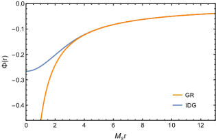
Figure 1: We have plotted the behavior of the potential $\Phi$ in IDG (blue line) and made a comparison with the corresponding one in the case of Reissner-Nordström metric in GR (orange line). We have chosen the values $G=1,m=1$ and $M_{s}=0.5$ and take $Q=0.5$.

is the Dawson function. Note that $\Phi\neq\Psi$, as it also happened in the GR case (see Appendix A). In the case $Q=0$ we recover the linearized IDG metric for a static neutral point-source derived in Ref. Biswas:2011ar , as expected. In the IR regime, $M_{s}r\gg 2$, the potentials in Eq. (13) reduce to those of the linearized Reissner-Nordström metric in GR, Eq. (48), as the asymptotic expansions for the Error function and the Dawson function are ${\rm Erf}(x)\sim 1$ and ${\rm F}(x)\sim 1/2x$. More interestingly, in the non-local regime, $M_{s}r\ll 2$, the metric potentials $\Phi(r)$ and $\Psi(r)$ approach non-singular constant values given by:

$$\begin{array}[]{ll}\lim\limits_{M_{s}r\to 0}\Phi(r)\equiv-A=\displaystyle-\frac{GmM_{s}}{\sqrt{\pi}}+\frac{1}{4}GQ^{2}M_{s}^{2},&\\ \lim\limits_{M_{s}r\to 0}\Psi(r)\equiv-B=\displaystyle-\frac{GmM_{s}}{\sqrt{\pi}}+\frac{1}{8}GQ^{2}M_{s}^{2},&\end{array}$$ (16)

because for $x\ll 1$ one has ${\rm Erf}(x)\sim 2x/\sqrt{\pi}$ and ${\rm F}(x)\sim x$. Note that when $Q=0$, we recover the case of neutral source, $A=B=GmM_{s}/\sqrt{\pi}$.

In Fig. 1 the potential $\Phi$ has been plotted as a function of $M_{s}r$ and a comparison between ghost-free IDG and GR has been made. We have chosen the values $G=1,m=1,$ $M_{s}=0.5$ and $Q=0.5$. It is also worth mentioning that the force per unit mass, $F_{g}(r)=-\partial\Phi/\partial r$, goes to zero linearly as a function of $r$. This vanishing force shows a classical aspect of asymptotic freedom in ghost-free IDG Biswas:2011ar .

Since we are working in the linearized regime, we need to satisfy the following two inequalities: $2|\Phi|<1$ and $2|\Psi|<1$. First of all, note that it is sufficient to focus just on one of the two inequalities, as the two metric potentials are almost the same apart from a factor $1/2$ appearing in the gravitational contribution due to the charge; see Eqs. (13,16). Moreover, for simplicity, we can drop all numerical factors and just focus on the essential parameters $m,$ $G=1/M_{p}^{2}$, $M_{s}$ and $Q.$

Mathematically, the weak-field inequality can be also satisfied when the neutral and charged contributions to the gravitational potential are both very large but such that the modulus of their sum is still less than one. However, from a physical point of view, in order to satisfy the weak-field inequalities, we need to require that both contributions have to be smaller than one Biswas:2011ar :

$$mM_{s}<M_{p}^{2},$$ (17)

$$Q^{2}M_{s}^{2}<M_{p}^{2}\Longleftrightarrow|Q|M_{s}<M_{p}.$$ (18)

We can immediately notice that, with respect to the neutral case, we now have the additional inequality in Eq. (18); together they will play a crucial role. In fact, we can make the following important observations.

• In the case of the Reissner-Nordström metric in Einstein’s GR one has to demand that the inequality

  $$|Q|\leq\frac{m}{M_{p}}$$ (19)

  always holds true in order to avoid the formation of a naked singularity during a collapsing phase. This is one example of the weak formulation of the cosmic censorship conjecture; see Refs. penrose ; hawking ; wald . In the case of a charged source in ghost-free IDG there is no need to require a cosmic censorship conjecture as the theory turns out to be singularity-free and devoid of any horizon as long as the inequalities in Eqs. (17,18) hold true.

• Thus, in Einstein’s GR one cannot describe the gravitational field generated by objects for which

  $$|Q|>\frac{m}{M_{p}},$$ (20)

  such as for an electron. In ghost-free IDG, both inequalities in Eqs. (19,20) are allowed. Indeed, consistently with the weak-field inequalities in Eqs. (17,20), we can have two possible scenarios:

  $$|Q|<\frac{m}{M_{p}}<\frac{M_{p}}{M_{s}}$$ (21)

  or

  $$\frac{m}{M_{p}}<|Q|<\frac{M_{p}}{M_{s}}.$$ (22)

  The most interesting case is the one described by the second inequality, Eq. (22), which says that in ghost-free IDG we can study the gravitational field of an object whose charge is bigger than its mass (in units of Planck mass), allowing us to include, for example, an electron in IDG.

• Finally, note that in the short-distance regime, $r<2/M_{s}$, one can in principle also have repulsive gravity, when

  $$Q^{2}M_{s}>m,$$

  and it is only compatible with the scenario in Eq. (22), and not with Eq. (21), as can be easily checked. However, such a repulsive contribution would be confined within the region of non-locality, while outside, gravity would be still attractive as in the standard GR.

IV Curvature tensors

We have computed all curvature tensors for the linearized IDG metric in Eqs. (9,13). All curvature expressions are evaluated up to first order in $G$, as we are working in the linear regime ($h_{\mu\nu}\sim G$). The full expressions are shown in Appendix C; instead, in this section we wish to emphasize that the presence of non-local gravitational interaction is such that all the curvatures tensors and invariants are regularized at the origin, i.e. at $r=0$. Therefore, we will focus on their forms in the region of non-locality, $r<2/M_{s}$.

In the non-local dominated regime, many components of the curvature tensors vanish, while the remaining tend to finite constant values at the origin. The non-zero components of the Riemann tensor are given by

$$\mathcal{R}_{0101}\sim\frac{1}{12}GM_{s}^{3}\left(\frac{2m}{\sqrt{\pi}}-Q^{2}M_{s}\right);\\$$ (23)

the non-zero components of the Ricci tensor:

$$\begin{array}[]{rl}\mathcal{R}_{00}\sim&\displaystyle\frac{1}{4}GM_{s}^{3}\left(\frac{2m}{\sqrt{\pi}}-Q^{2}M_{s}\right),\\ \mathcal{R}_{11}\sim&\displaystyle\frac{1}{12}GM_{s}^{3}\left(\frac{6m}{\sqrt{\pi}}-Q^{2}M_{s}\right);\end{array}$$ (24)

and the Ricci scalar:

$$\mathcal{R}\sim\frac{GmM_{s}^{3}}{\sqrt{\pi}}.$$ (25)

Finally, we note that all components of the Weyl tensor tend to zero at the origin, as we take $M_{s}r\rightarrow 0$:

$$\mathcal{C}_{\mu\nu\rho\sigma}\sim 0,$$ (26)

Important point to note that with decreasing distance, different components of the Weyl tensor approach zero with different rates, particularly $O(r^{2})$, $O(r^{4})$ and $O(r^{6})$ for small $r$, such that very close to the origin, we can imagine a constant valley, and the metric becomes exactly conformally-flat at $r=0$. This implies that the static metric of a charged source approaches conformal-flatness in the UV regime, $r<2/M_{s}.$ In fact, in the short distance regime, the metric in Eqs. (9,13) can be approximated to:

$$ds^{2}\approx-(1-2A)dt^{2}+(1+2B)(dr^{2}+r^{2}d\Omega^{2}),$$ (27)

which can be put in a conformally-flat form by introducing a conformal time, $\tau$, through the following coordinate transformation

$$\tau=\sqrt{\frac{1-2A}{1+2B}}t;$$ (28)

such that the metric in the non-local region reads

$$\begin{array}[]{rl}ds^{2}=&(1+2B)\left[-d\tau^{2}+dr^{2}+r^{2}d\Omega^{2}\right]\\ =&F^{2}\eta,\end{array}$$ (29)

where $\eta$ is the Minkowski metric and $F^{2}\equiv 1+2B>0$ is the conformal factor. In Fig. 2 we have plotted the component $\mathcal{C}_{0101}$ of the Weyl tensor for both the charged case in ghost-free IDG and Reissner-Nordström in GR.

We can note that, by setting $Q=0$ we recover the curvature tensors for the ghost-free IDG neutral case obtained in Ref. Buoninfante:2018xiw , as expected. Furthermore, we have computed all the curvature invariants squared. Their full expressions are shown in Appendix C, while in this section we will present their values in the non-local region. In the non-local regime, $r<2/M_{s},$ the Kretschmann scalar $\mathcal{K}=\mathcal{R}_{\mu\nu\rho\sigma}\mathcal{R}^{\mu\nu\rho\sigma}$ tends to the following finite constant value as $M_{s}r\rightarrow 0$:

$$\mathcal{K}\sim\frac{G^{2}M_{s}^{6}\left(10m^{2}-6\sqrt{\pi}mQ^{2}M_{s}+\pi Q^{4}M_{s}^{2}\right)}{6\pi}.$$ (30)

In Fig. 3 we see explicitly that the Kretschmann invariant for a charged source in ghost-free IDG is regularized at the origin, unlike the case of Reissner Nordström in GR where we have a curvature singularity.

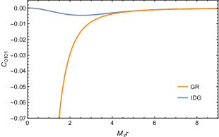
(a) Subfigure 1 list of figures text

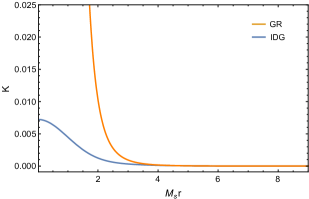
(b) Subfigure 2 list of figures text

Figure 2: We have shown the spacetime properties of ghost-free IDG (blue line) and GR (orange line) as functions of $M_{s}r$: (a) $\mathcal{C}_{0101}$ component of the Weyl tensor and (b) the Kretschmann scalar $\mathcal{K}$. We have set $M_{p}=1,\leavevmode\nobreak\ m=1,$ $M_{s}=0.5$ and $Q=0.5$. In these units the Schwarzschild radius is $r_{sch}=2$. Note that, unlike in GR where the linearized approximation would break down for $r\leq 2$, in the case of ghost-free IDG we can smoothly approach $r=0$, provided $mM_{s}<M_{p}^{2}$ and $|Q|M_{s}<M_{p}.$ From these two plots it is obvious that the presence of non-locality helps to avoid the curvature-singularities at the origin.

Moreover, in the non-local region, as $M_{s}r\rightarrow 0$, the non-zero components of the Ricci scalar squared and the Ricci tensor squared are given by the following finite constant values:

$$\mathcal{R}^{2}\sim\frac{G^{2}m^{2}M_{s}^{6}}{\pi},$$ (31)

$$\mathcal{R}_{\mu\nu}\mathcal{R}^{\mu\nu}\sim\frac{G^{2}M_{s}^{6}\left(12m^{2}-6\sqrt{\pi}mQ^{2}M_{s}+\pi Q^{4}M_{s}^{2}\right)}{12\pi}.$$ (32)

While the Weyl tensor squared vanishes at the origin:

$$\mathcal{C}_{\mu\nu\rho\sigma}\mathcal{C}^{\mu\nu\rho\sigma}\sim 0.$$ (33)

For completeness, it can be checked that the squared curvatures satisfy the following identity:

$$\mathcal{C}_{\mu\nu\rho\sigma}\mathcal{C}^{\mu\nu\rho\sigma}=\frac{\mathcal{R}^{2}}{3}-2\mathcal{R}_{\mu\nu}\mathcal{R}^{\mu\nu}+\mathcal{K}.$$ (34)

Needless to say, all the curvature invariants for the case of a point-charge source in ghost-free IDG reduce to those of the uncharged case, $Q=0$, obtained in Ref. Buoninfante:2018xiw , as expected.

V Conclusions

In this paper we have found a linearized static metric solution for an electric point-charge in ghost-free IDG whose action is governed by Ref.Biswas:2011ar . We have noticed that all the features of the case of neutral source are still kept; indeed the metric turns out to be regular at the origin and all curvature invariants are singularity-free. Moreover, all components of the Weyl tensor tend to zero as $M_{s}r\rightarrow 0$, meaning that the spacetime metric approaches conformal-flatness in the non-local regime.

We have also argued that in ghost-free IDG there is no need to require the cosmic censorship conjecture as the spacetime is singularity-free and devoid of any horizon as long as the inequalities in Eqs. (17,18) hold true. Moreover, unlike the case of Reissner-Nordström in GR, in ghost-free IDG no constraint has to be imposed on the relation between mass and charge of the source. Indeed, we can have cases where $|Q|>m/M_{p}$ is satisfied, allowing us to include in the theory objects such as an electron. Furthermore, we would expect that massive compact charged systems, devoid of singularity and event horizons can be found in this case too, similar to the case of neutral source studied in Ref.Koshelev:2017bxd .

Appendix A Reissner-Nordström metric in Einstein’s general relativity

In this appendix we wish to briefly review the main aspects of the Reissner-Nordström metric in GR; in particular we will introduce its form in the isotropic coordinates which is usually not studied in the standard text-books. The Reissner-Nordström metric is a non-vacuum solution of the full non-linear Einstein equations:

$$\mathcal{R}_{\mu\nu}-\frac{1}{2}g_{\mu\nu}\mathcal{R}=8\pi G\tau_{\mu\nu},$$ (35)

where $\tau_{\mu\nu}$ is the electro-magnetic energy momentum tensor

$$\tau_{\mu\nu}=\frac{1}{4\pi}\left(\eta_{\rho\nu}F_{\mu\sigma}F^{\rho\sigma}-\frac{1}{4}\eta_{\mu\nu}F_{\rho\sigma}F^{\rho\sigma}\right).$$ (36)

Assuming that no magnetic monopole is present, the only components of the field strength $F_{\mu\nu}$ will be given by the electric field part; then, due to spherical symmetry there will be a radial dependence so that the only non-vanishing components are $F_{10}=-F_{01}=Q/r^{2}.$ In the Schwarzschild coordinates $(t,R,\theta,\varphi)$, where $R$ is the polar radial coordinate, the metric reads

$$\begin{array}[]{rl}ds^{2}=&\displaystyle-\left(1-\frac{2Gm}{R}+\frac{GQ^{2}}{R^{2}}\right)dt^{2}\\ &\displaystyle+\left(1-\frac{2Gm}{R}+\frac{GQ^{2}}{R^{2}}\right)^{-1}dR^{2}+R^{2}d\Omega^{2},\end{array}$$ (37)

where $d\Omega^{2}\equiv d\theta^{2}+{\rm sin}^{2}\theta d\varphi^{2}$, $m$ and $Q$ are the mass and the charge of the source, respectively.

One can immediately notice that the Reissner-Nordström metric posses two horizons that are defined as:

$$r_{\pm}=Gm\pm\sqrt{G^{2}m^{2}-GQ^{2}},$$ (38)

where $r_{+}$ is called outer horizon, while $r_{-}$ inner horizon.

We are now interested in finding the corresponding weak-field approximation for the metric in Eq. (37) and to do so, as it happens for the Schwarzschild metric, it is more convenient to use the isotropic coordinates $(t,r,\theta,\varphi)$, where $r$ is the isotropic radial coordinate that in the case of Reissner-Nordström metric is defined by the following transformation:

$$R=r\left[\left(1+\frac{Gm}{2r}\right)^{2}-\frac{GQ^{2}}{4r^{2}}\right].$$ (39)

In isotropic coordinates the metric in Eq. (37) becomes:

$$\begin{array}[]{rl}ds^{2}=&\displaystyle-\left[\frac{1-\left(\frac{Gm}{2r}\right)^{2}+\frac{GQ^{2}}{4r^{2}}}{\left(1+\frac{Gm}{2r}\right)^{2}-\frac{GQ^{2}}{4r^{2}}}\right]^{2}dt^{2}\\ &\displaystyle+\left[\left(1+\frac{Gm}{2r}\right)-\frac{GQ^{2}}{4r^{2}}\right]^{2}(dr^{2}+r^{2}d\Omega^{2});\end{array}$$ (40)

it is evident that for $Q=0$ we recover the Schwarzschild metric in isotropic coordinates.

We can now make an expansion for weak gravitational field and stop at the linear order in $G$, thus the metric in Eq. (40) in the linearized regime reads:

$$\begin{array}[]{rl}ds^{2}=&\displaystyle-\left(1-\frac{2Gm}{r}+\frac{GQ^{2}}{r^{2}}\right)dt^{2}\\ &\displaystyle+\left(1+\frac{2Gm}{r}-\frac{GQ^{2}}{2r^{2}}\right)(dr^{2}+r^{2}d\Omega^{2}).\end{array}$$ (41)

It is very important to stress that the metric in Eq. (41) can be also obtained with a different procedure, i.e. by perturbing the metric around a Minkowski background and working in the linear regime:

$$g_{\mu\nu}(x)=\eta_{\mu\nu}+h_{\mu\nu}(x),$$ (42)

so that the Einstein field equations in Eq. (35) in the linear regime are given by:

$$\begin{array}[]{ll}\displaystyle\Box h_{\mu\nu}+(\eta_{\mu\nu}\partial_{\rho}\partial_{\sigma}h^{\rho\sigma}+\partial_{\mu}\partial_{\nu}h)&\\ \,\,\,\,\,\,\,\,\,\,\,\displaystyle-\partial_{\sigma}(\partial_{\nu}h^{\sigma}_{\mu}+\partial_{\mu}h_{\nu}^{\sigma})-\eta_{\mu\nu}\Box h=-16\pi G\tau_{\mu\nu}.&\end{array}$$ (43)

By working in a weak field regime and considering the case of a static source, the spacetime metric can be written as:

$$ds^{2}=-(1+2\Phi(r))dt^{2}+(1-2\Psi(r))(dr^{2}+r^{2}d\Omega^{2}),$$ (44)

where $r$ is the isotropic radial coordinate; thus the only two unknowns we need to find are the two gravitational potentials $\Phi$ and $\Psi$. By looking at the $00$-component and the trace of the linearized field equations in Eq. (43) we obtain:

$$\begin{array}[]{rl}\displaystyle\nabla^{2}h_{00}-\partial_{i}\partial_{j}h^{ij}+\nabla^{2}h=&-16\pi G\tau_{00},\\ \displaystyle-2\nabla^{2}h+2\partial_{i}\partial_{j}h^{ij}=&-16\pi G\tau.\end{array}$$ (45)

Using $h=2(\Phi-3\Psi),$ $h_{00}=-2\Phi$ and $h_{ii}=-2\Psi$ we obtain two differential equations for the two gravitational fields $\Phi$ and $\Psi$:

$$\begin{array}[]{rl}\displaystyle\nabla^{2}\Phi=&4\pi G(\tau+2\tau_{00}),\\ \displaystyle\nabla^{2}\Psi=&4\pi G\tau_{00}.\end{array}$$ (46)

In the case of a charged static source, the energy-momentum tensor turns out to be traceless, $\tau=0,$ while the $00$-component is given by $\tau_{00}=Q^{2}/8\pi r^{4}.$ We can now solve the two differential equations in Eq. (46) and obtain:

$$\begin{array}[]{rl}\displaystyle\Phi(r)=&\displaystyle-\frac{C_{1}}{r}+\frac{GQ^{2}}{2r^{2}}+C_{2},\\ \displaystyle\Psi(r)=&\displaystyle-\frac{C_{1}}{r}+\frac{GQ^{2}}{4r^{2}}+C_{2},\end{array}$$ (47)

where $C_{1}$ and $C_{2}$ are two integration constants whose value can be fixed by imposing physical suitable boundary conditions. First of all, for $r=\infty$ we want that $\Phi$ and $\Psi$ are zero (asymptotic flatness) which means $C_{2}=0$; while $C_{1}$ can be found by imposing that for $Q=0$ we have the usual Newtonian potential, thus $C_{1}=Gm:$

$$\begin{array}[]{rl}\displaystyle\Phi(r)=&-\displaystyle\frac{Gm}{r}+\frac{GQ^{2}}{2r^{2}},\\ \displaystyle\Psi(r)=&-\displaystyle\frac{Gm}{r}+\frac{GQ^{2}}{4r^{2}}.\end{array}$$ (48)

Notice that in the case of a charged source $\Phi\neq\Psi$. It is clear that the linearized metric in Eq. (44) with the gravitational fields derived in Eq. (48) coincides with the metric in Eq. (41) which we derived instead by starting from the full non-linear Reissner-Nordström metric. It is very important to note that in the weak field approximation one has $2|\Phi|,2|\Psi|<1,$ which means that the radial coordinate has to always be greater than the outer horizon radius, $r>r_{+}$. Thus, in Einstein’s GR it so happens that the linear approximation breaks down once one approaches the horizon. As we have seen in the paper, this is not the case for infinite derivative gravity, where (for both charged and neutral sources) the linear regime holds all the way up to $r=0.$

Appendix B Working with infinite order differential equations

We can solve the differential equations in Eq. (12) in several ways, for example by making the following temporary field-redefinitions:

$$\bar{\Phi}:=e^{-\nabla^{2}/M_{s}^{2}}\Phi,\,\,\,\,\,\,\,\,\,\,\,\bar{\Psi}:=e^{-\nabla^{2}/M_{s}^{2}}\Psi,$$ (49)

so that the equations in (42) become

$$\begin{array}[]{rl}\displaystyle\nabla^{2}\bar{\Phi}(r)=&\displaystyle\frac{GQ^{2}}{r^{4}}\\ \displaystyle\nabla^{2}\bar{\Psi}(r)=&\displaystyle\frac{GQ^{2}}{2r^{4}}.\end{array}$$ (50)

The structure of these equations is similar to the one we have in the case of a charged source in Einstein’s GR, i.e. Reissner-Nordström, as also shown in Appendix A in Eq. (46); thus the solution will be also of the same structure as the one in Eq. (47):

$$\begin{array}[]{rl}\displaystyle\bar{\Phi}(r)=&\displaystyle-\frac{C_{1}}{r}+\frac{GQ^{2}}{2r^{2}}+C_{2}\\ \displaystyle\bar{\Psi}(r)=&\displaystyle-\frac{C_{1}}{r}+\frac{GQ^{2}}{4r^{2}}+C_{2}.\end{array}$$ (51)

By requiring the boundary conditions of asymptotic flatness one gets $C_{2}=0;$ while $C_{1}$ can be fixed that for $Q=0$ one recovers the case of neutral point-source, which means $C_{1}=Gm$. In terms of the real fields $\Phi$ and $\Psi$, Eq. (49) will give:

$$\begin{array}[]{rl}\displaystyle\Phi(r)=&\displaystyle-Gme^{\nabla^{2}/M_{s}^{2}}\left(\frac{1}{r}\right)+\frac{GQ^{2}}{2}e^{\nabla^{2}/M_{s}^{2}}\left(\frac{1}{r^{2}}\right)\\ \displaystyle\Psi(r)=&\displaystyle-Gme^{\nabla^{2}/M_{s}^{2}}\left(\frac{1}{r}\right)+\frac{GQ^{2}}{4}e^{\nabla^{2}/M_{s}^{2}}\left(\frac{1}{r^{2}}\right)\end{array}$$ (52)

We now need to compute the action of the exponential $e^{-\nabla^{2}/M_{s}^{2}}$ on the functions $1/r$ and $1/r^{2}$. Notice that:

$$\begin{array}[]{rl}\displaystyle e^{\nabla^{2}/M_{s}^{2}}\left(\frac{1}{r}\right)=&\displaystyle e^{\nabla^{2}/M_{s}^{2}}\int\frac{d^{3}k}{(2\pi)^{3}}\frac{4\pi}{k^{2}}e^{i\vec{k}\cdot\vec{r}}\\ =&\displaystyle\int\frac{d^{3}k}{(2\pi)^{3}}\frac{4\pi}{k^{2}}e^{-k^{2}/M_{s}^{2}}e^{i\vec{k}\cdot\vec{r}}\\ =&\displaystyle\frac{2}{\pi}\int_{0}^{\infty}dk\ \frac{\sin{(kr)}}{kr}e^{-k^{2}/M_{s}^{2}}\\ =&\displaystyle\frac{1}{r}{\rm Erf}\left(\frac{M_{s}r}{2}\right),\end{array}$$ (53)

where we have used the fact that $4\pi/k^{2}$ is the Fourier transform of $1/r$. We can proceed in the same way to compute the second contribution, indeed by noting that the Fourier transform of $1/r^{2}$ is $\frac{2\pi^{2}}{k}{\rm sign}(k)$, one has:

$$\begin{array}[]{rl}\displaystyle e^{\nabla^{2}/M_{s}^{2}}\left(\frac{1}{r^{2}}\right)=&\displaystyle e^{\nabla^{2}/M_{s}^{2}}\int\frac{d^{3}k}{(2\pi)^{3}}\frac{2\pi^{2}}{k}{\rm sign}(k)e^{i\vec{k}\cdot\vec{r}}\\ =&\displaystyle\int\frac{d^{3}k}{(2\pi)^{3}}\frac{2\pi^{2}}{k}{\rm sign}(k)e^{-k^{2}/M_{s}^{2}}e^{i\vec{k}\cdot\vec{r}}\\ =&\displaystyle\int_{0}^{\infty}dk\ \frac{\sin{(kr)}}{r}e^{-k^{2}/M_{s}^{2}}\\ =&\displaystyle\frac{M_{s}}{r}{\rm F}\left(\frac{M_{s}r}{2}\right),\end{array}$$ (54)

where ${\rm F}(M_{s}r/2)$ is the Dawson function.

Thus, by using Eqs. (53,54), we can now obtain the expressions for the two metric potentials in Eq. (13).

Appendix C Full expressions of the curvature tensors

In this appendix we show the full expressions for all curvature tensors and invariants for the IDG linearized static metric for a charged point-source derived in Eqs. (9,13).

The Ricci scalar is given by:

$$\mathcal{R}=\frac{GmM_{s}^{3}e^{-\frac{1}{4}r^{2}M_{s}^{2}}}{\sqrt{\pi}};$$ (55)

the non-zero components of the Riemann tensor:

$$\begin{array}[]{rl}\mathcal{R}_{0101}=&\displaystyle\frac{1}{8}G\Bigg{[}M_{s}^{3}\left(\frac{2Q^{2}\text{F}\left(\frac{rM_{s}}{2}\right)}{r}+\frac{4me^{-\frac{1}{4}r^{2}M_{s}^{2}}}{\sqrt{\pi}}\right)+\frac{8M_{s}\left(Q^{2}\text{F}\left(\frac{rM_{s}}{2}\right)+\frac{2mre^{-\frac{1}{4}r^{2}M_{s}^{2}}}{\sqrt{\pi}}\right)}{r^{3}}\\ &+\displaystyle Q^{2}rM_{s}^{5}\text{F}\left(\frac{rM_{s}}{2}\right)-\frac{16m\text{Erf}\left(\frac{rM_{s}}{2}\right)}{r^{3}}-\frac{4Q^{2}M_{s}^{2}}{r^{2}}-Q^{2}M_{s}^{4}\Bigg{]},\\ \mathcal{R}_{0303}=&\displaystyle\mathcal{R}_{0202}\sin^{2}(\theta)\\ =&\displaystyle\frac{1}{4}G\sin^{2}(\theta)\left[M_{s}\left(-\frac{2Q^{2}\text{F}\left(\frac{rM_{s}}{2}\right)}{r}-\frac{4me^{-\frac{1}{4}r^{2}M_{s}^{2}}}{\sqrt{\pi}}\right)-Q^{2}rM_{s}^{3}\text{F}\left(\frac{rM_{s}}{2}\right)+\frac{4m\text{Erf}\left(\frac{rM_{s}}{2}\right)}{r}+Q^{2}M_{s}^{2}\right],\\ \mathcal{R}_{1313}=&\displaystyle\mathcal{R}_{1212}\sin^{2}(\theta)\\ =&\displaystyle\frac{1}{16}G\sin^{2}(\theta)\Bigg{[}M_{s}\left(\frac{4Q^{2}\text{F}\left(\frac{rM_{s}}{2}\right)}{r}+\frac{16me^{-\frac{1}{4}r^{2}M_{s}^{2}}}{\sqrt{\pi}}\right)+Q^{2}r^{3}M_{s}^{5}\text{F}\left(\frac{rM_{s}}{2}\right)-\frac{16m\text{Erf}\left(\frac{rM_{s}}{2}\right)}{r}\\ &+\displaystyle\frac{8mr^{2}M_{s}^{3}e^{-\frac{1}{4}r^{2}M_{s}^{2}}}{\sqrt{\pi}}-Q^{2}r^{2}M_{s}^{4}-2Q^{2}M_{s}^{2}\Bigg{]},\\ \mathcal{R}_{2323}=&\displaystyle\frac{1}{4}Gr\sin^{2}(\theta)\Bigg{[}M_{s}\left(-2Q^{2}\text{F}\left(\frac{rM_{s}}{2}\right)-\frac{8mre^{-\frac{1}{4}r^{2}M_{s}^{2}}}{\sqrt{\pi}}\right)-Q^{2}r^{2}M_{s}^{3}\text{F}\left(\frac{rM_{s}}{2}\right)\\ &+\displaystyle 8m\text{Erf}\left(\frac{rM_{s}}{2}\right)+Q^{2}rM_{s}^{2}\Bigg{]};\end{array}$$ (56)

the non-zero components of the Ricci tensor:

$$\begin{array}[]{rl}\mathcal{R}_{00}=&\displaystyle\frac{1}{8}GM_{s}^{3}\left[\frac{Q^{2}\left(r^{2}M_{s}^{2}-2\right)\text{F}\left(\frac{rM_{s}}{2}\right)}{r}+\frac{4me^{-\frac{1}{4}r^{2}M_{s}^{2}}}{\sqrt{\pi}}-Q^{2}M_{s}\right],\\ \mathcal{R}_{11}=&\displaystyle\frac{1}{4}GM_{s}\left[M_{s}\left(\frac{2mM_{s}e^{-\frac{1}{4}r^{2}M_{s}^{2}}}{\sqrt{\pi}}+\frac{Q^{2}}{r^{2}}\right)-\frac{Q^{2}\left(r^{2}M_{s}^{2}+2\right)\text{F}\left(\frac{rM_{s}}{2}\right)}{r^{3}}\right],\\ \mathcal{R}_{22}=&\displaystyle\frac{1}{16}GM_{s}\left[\frac{Q^{2}\left(r^{4}M_{s}^{4}+4\right)\text{F}\left(\frac{rM_{s}}{2}\right)}{r}+M_{s}\left(\frac{8mr^{2}M_{s}e^{-\frac{1}{4}r^{2}M_{s}^{2}}}{\sqrt{\pi}}-Q^{2}r^{2}M_{s}^{2}-2Q^{2}\right)\right],\\ \mathcal{R}_{33}=&\displaystyle\frac{1}{16}G\sin^{2}(\theta)M_{s}\left[\frac{Q^{2}\left(r^{4}M_{s}^{4}+4\right)\text{F}\left(\frac{rM_{s}}{2}\right)}{r}+M_{s}\left(\frac{8mr^{2}M_{s}e^{-\frac{1}{4}r^{2}M_{s}^{2}}}{\sqrt{\pi}}-Q^{2}r^{2}M_{s}^{2}-2Q^{2}\right)\right];\end{array}$$ (57)

the non-zero components of the Weyl tensor:

$$\begin{array}[]{rl}\mathcal{C}_{0101}=&\displaystyle\frac{1}{48}G\Bigg{[}M_{s}^{3}\left(\frac{12Q^{2}\text{F}\left(\frac{rM_{s}}{2}\right)}{r}+\frac{16me^{-\frac{1}{4}r^{2}M_{s}^{2}}}{\sqrt{\pi}}\right)+\frac{M_{s}\left(36Q^{2}\text{F}\left(\frac{rM_{s}}{2}\right)+\frac{96mre^{-\frac{1}{4}r^{2}M_{s}^{2}}}{\sqrt{\pi}}\right)}{r^{3}}\\ &+\displaystyle 3Q^{2}rM_{s}^{5}\text{F}\left(\frac{rM_{s}}{2}\right)-\frac{96m\text{Erf}\left(\frac{rM_{s}}{2}\right)}{r^{3}}-\frac{18Q^{2}M_{s}^{2}}{r^{2}}-3Q^{2}M_{s}^{4}\Bigg{]},\\ \mathcal{C}_{0303}=&-\displaystyle\mathcal{C}_{1313}=\mathcal{C}_{0202}\sin^{2}(\theta)=-\mathcal{C}_{1212}\sin^{2}(\theta)\\ =&\displaystyle\frac{1}{96}G\sin^{2}(\theta)\Bigg{[}4rM_{s}^{3}\left(-3Q^{2}\text{F}\left(\frac{rM_{s}}{2}\right)-\frac{4mre^{-\frac{1}{4}r^{2}M_{s}^{2}}}{\sqrt{\pi}}\right)+M_{s}\left(-\frac{36Q^{2}\text{F}\left(\frac{rM_{s}}{2}\right)}{r}-\frac{96me^{-\frac{1}{4}r^{2}M_{s}^{2}}}{\sqrt{\pi}}\right)\\ &-\displaystyle 3Q^{2}r^{3}M_{s}^{5}\text{F}\left(\frac{rM_{s}}{2}\right)+\frac{96m\text{Erf}\left(\frac{rM_{s}}{2}\right)}{r}+3Q^{2}r^{2}M_{s}^{4}+18Q^{2}M_{s}^{2}\Bigg{]},\\ \mathcal{C}_{2323}=&\displaystyle\frac{1}{48}Gr\sin^{2}(\theta)\Bigg{[}4r^{2}M_{s}^{3}\left(-3Q^{2}\text{F}\left(\frac{rM_{s}}{2}\right)-\frac{4mre^{-\frac{1}{4}r^{2}M_{s}^{2}}}{\sqrt{\pi}}\right)+M_{s}\left(-36Q^{2}\text{F}\left(\frac{rM_{s}}{2}\right)-\frac{96mre^{-\frac{1}{4}r^{2}M_{s}^{2}}}{\sqrt{\pi}}\right)\\ &-\displaystyle 3Q^{2}r^{4}M_{s}^{5}\text{F}\left(\frac{rM_{s}}{2}\right)+96m\text{Erf}\left(\frac{rM_{s}}{2}\right)+3Q^{2}r^{3}M_{s}^{4}+18Q^{2}rM_{s}^{2}\Bigg{]}.\end{array}$$ (58)

We will now show the expressions for the curvature invariants. The Ricci scalar squared is given by:

$$\mathcal{R}^{2}=\displaystyle\frac{G^{2}m^{2}M_{s}^{6}e^{-\frac{1}{2}r^{2}M_{s}^{2}}}{\pi};\\$$ (59)

the Ricci tensor squared:

$$\begin{array}[]{rl}\mathcal{R}_{\mu\nu}\mathcal{R}^{\mu\nu}=&\displaystyle\frac{G^{2}M_{s}^{2}}{128\pi r^{6}}\Bigg{[}\text{F}\left(\frac{rM_{s}}{2}\right)\Bigg{(}32\sqrt{\pi}mQ^{2}r^{7}M_{s}^{6}e^{-\frac{1}{4}r^{2}M_{s}^{2}}-64\sqrt{\pi}mQ^{2}r^{5}M_{s}^{4}e^{-\frac{1}{4}r^{2}M_{s}^{2}}\\ &\displaystyle-6\pi Q^{4}r^{7}M_{s}^{7}+4\pi Q^{4}r^{5}M_{s}^{5}-24\pi Q^{4}r^{3}M_{s}^{3}-48\pi Q^{4}rM_{s}\Bigg{)}\\ &\displaystyle+\pi Q^{4}\left(3r^{8}M_{s}^{8}-8r^{6}M_{s}^{6}+24r^{4}M_{s}^{4}+32r^{2}M_{s}^{2}+48\right)\text{F}\left(\frac{rM_{s}}{2}\right)^{2}\\ &+\displaystyle M_{s}^{4}\left(128m^{2}r^{6}e^{-\frac{1}{2}r^{2}M_{s}^{2}}+4\pi Q^{4}r^{4}\right)-32\sqrt{\pi}mQ^{2}r^{6}M_{s}^{5}e^{-\frac{1}{4}r^{2}M_{s}^{2}}+3\pi Q^{4}r^{6}M_{s}^{6}+12\pi Q^{4}r^{2}M_{s}^{2}\Bigg{]};\end{array}$$ (60)

the Weyl tensor squared:

$$\begin{array}[]{rl}\mathcal{C}_{\mu\nu\rho\sigma}\mathcal{C}^{\mu\nu\rho\sigma}=&\displaystyle\frac{G^{2}e^{-\frac{1}{2}r^{2}M_{s}^{2}}}{192\pi r^{6}}\Bigg{[}-4r^{2}M_{s}^{3}\left(3\sqrt{\pi}Q^{2}e^{\frac{1}{4}r^{2}M_{s}^{2}}\text{F}\left(\frac{rM_{s}}{2}\right)+4mr\right)\\ &-\displaystyle 12M_{s}\left(3\sqrt{\pi}Q^{2}e^{\frac{1}{4}r^{2}M_{s}^{2}}\text{F}\left(\frac{rM_{s}}{2}\right)+8mr\right)\\ &-\displaystyle 3\sqrt{\pi}Q^{2}r^{4}M_{s}^{5}e^{\frac{1}{4}r^{2}M_{s}^{2}}\text{F}\left(\frac{rM_{s}}{2}\right)+96\sqrt{\pi}me^{\frac{1}{4}r^{2}M_{s}^{2}}\text{Erf}\left(\frac{rM_{s}}{2}\right)\\ &+\displaystyle 18\sqrt{\pi}Q^{2}rM_{s}^{2}e^{\frac{1}{4}r^{2}M_{s}^{2}}+3\sqrt{\pi}Q^{2}r^{3}M_{s}^{4}e^{\frac{1}{4}r^{2}M_{s}^{2}}\Bigg{]}^{2};\end{array}$$ (61)

and the Kretschmann invariant:

$$\begin{array}[]{rl}\mathcal{K}=&\displaystyle\frac{e^{-\frac{1}{2}r^{2}M_{s}^{2}}G^{2}}{32\pi r^{6}}\Bigg{[}3e^{\frac{1}{2}r^{2}M_{s}^{2}}\pi Q^{4}r^{8}{\rm F}\left(\frac{rM_{s}}{2}\right){}^{2}M_{s}^{10}-6e^{\frac{1}{2}r^{2}M_{s}^{2}}\pi Q^{4}r^{7}{\rm F}\left(\frac{rM_{s}}{2}\right)M_{s}^{9}\\ &+\displaystyle\left(32e^{\frac{1}{4}r^{2}M_{s}^{2}}m\sqrt{\pi}Q^{2}{\rm F}\left(\frac{rM_{s}}{2}\right)r^{7}+3e^{\frac{1}{2}r^{2}M_{s}^{2}}\pi Q^{4}r^{6}+8e^{\frac{1}{2}r^{2}M_{s}^{2}}\pi Q^{4}{\rm F}\left(\frac{rM_{s}}{2}\right){}^{2}r^{6}\right)M_{s}^{8}\\ &-\displaystyle 4e^{\frac{1}{4}r^{2}M_{s}^{2}}\sqrt{\pi}Q^{2}r^{5}\left(7e^{\frac{1}{4}r^{2}M_{s}^{2}}\sqrt{\pi}{\rm F}\left(\frac{rM_{s}}{2}\right)Q^{2}+8mr\right)M_{s}^{7}\\ &+\displaystyle 4r^{4}\left(18e^{\frac{1}{2}r^{2}M_{s}^{2}}\pi{\rm F}\left(\frac{rM_{s}}{2}\right){}^{2}Q^{4}+5e^{\frac{1}{2}r^{2}M_{s}^{2}}\pi Q^{4}+32e^{\frac{1}{4}r^{2}M_{s}^{2}}m\sqrt{\pi}r{\rm F}\left(\frac{rM_{s}}{2}\right)Q^{2}+24m^{2}r^{2}\right)M_{s}^{6}\\ &-\displaystyle 24e^{\frac{1}{4}r^{2}M_{s}^{2}}\sqrt{\pi}Q^{2}r^{3}\left(8mr+e^{\frac{1}{4}r^{2}M_{s}^{2}}\sqrt{\pi}{\rm F}\left(\frac{rM_{s}}{2}\right)\left(5Q^{2}+4mr\text{Erf}\left(\frac{rM_{s}}{2}\right)\right)\right)M_{s}^{5}\\ &+\displaystyle 4r^{2}\bigg{(}40e^{\frac{1}{2}r^{2}M_{s}^{2}}\pi{\rm F}\left(\frac{rM_{s}}{2}\right){}^{2}Q^{4}+15e^{\frac{1}{2}r^{2}M_{s}^{2}}\pi Q^{4}+144e^{\frac{1}{4}r^{2}M_{s}^{2}}m\sqrt{\pi}r{\rm F}\left(\frac{rM_{s}}{2}\right)Q^{2}\\ &\displaystyle+24e^{\frac{1}{2}r^{2}M_{s}^{2}}m\pi r\text{Erf}\left(\frac{rM_{s}}{2}\right)Q^{2}+128m^{2}r^{2}\bigg{)}M_{s}^{4}\\ &\displaystyle-16e^{\frac{1}{4}r^{2}M_{s}^{2}}\sqrt{\pi}r\bigg{(}3e^{\frac{1}{4}r^{2}M_{s}^{2}}\sqrt{\pi}{\rm F}\left(\frac{rM_{s}}{2}\right)\left(5Q^{2}+8mr\text{Erf}\left(\frac{rM_{s}}{2}\right)\right)Q^{2}\\ &+\displaystyle 4mr\left(9Q^{2}+8mr\text{Erf}\left(\frac{rM_{s}}{2}\right)\right)\bigg{)}M_{s}^{3}+48\bigg{(}5e^{\frac{1}{2}r^{2}M_{s}^{2}}\pi{\rm F}\left(\frac{rM_{s}}{2}\right){}^{2}Q^{4}\\ &\displaystyle+24e^{\frac{1}{4}r^{2}M_{s}^{2}}m\sqrt{\pi}r{\rm F}\left(\frac{rM_{s}}{2}\right)Q^{2}+\displaystyle 4mr\left(3e^{\frac{1}{2}r^{2}M_{s}^{2}}\pi\text{Erf}\left(\frac{rM_{s}}{2}\right)Q^{2}+8mr\right)\bigg{)}M_{s}^{2}\\ &-\displaystyle 384e^{\frac{1}{4}r^{2}M_{s}^{2}}m\sqrt{\pi}\left(3e^{\frac{1}{4}r^{2}M_{s}^{2}}\sqrt{\pi}{\rm F}\left(\frac{rM_{s}}{2}\right)Q^{2}+8mr\right)\text{Erf}\left(\frac{rM_{s}}{2}\right)M_{s}+1536e^{\frac{1}{2}r^{2}M_{s}^{2}}m^{2}\pi\text{Erf}\left(\frac{rM_{s}}{2}\right)^{2}\Bigg{]}.\end{array}$$ (62)

In the case $Q=0$, we would recover all curvature tensors and invariants for the case of a neutral point-source obtained in Ref. Buoninfante:2018xiw , as expected.

References

- (1) C. M. Will, Living Rev. Rel. 17, 4 (2014) [arXiv:1403.7377 [gr-qc]].
- (2) B. P. Abbott et al. [LIGO Scientific and Virgo Collaborations], Phys. Rev. Lett. 116 (2016) no.6, 061102.
- (3) K. S. Stelle, Phys. Rev. D 16 (1977) 953.
- (4) T. Biswas, A. Mazumdar and W. Siegel, “Bouncing universes in string-inspired gravity,” JCAP 0603, 009 (2006) [hep-th/0508194].
- (5) T. Biswas, E. Gerwick, T. Koivisto and A. Mazumdar, “Towards singularity and ghost-free theories of gravity,” Phys. Rev. Lett. 108, 031101 (2012).
- (6) Yu. V. Kuzmin, Yad. Fiz. 50, 1630-1635 (1989).
- (7) E. Tomboulis, Phys. Lett. B 97, 77 (1980). E. T. Tomboulis, Renormalization And Asymptotic Freedom In Quantum Gravity, In *Christensen, S.m. ( Ed.): Quantum Theory Of Gravity*, 251-266. E. T. Tomboulis, Superrenormalizable gauge and gravitational theories, hep- th/9702146;
- (8) A. A. Tseytlin, “On singularities of spherically symmetric backgrounds in string theory,” Phys. Lett. B 363, 223 (1995) [hep-th/9509050].
- (9) W. Siegel, “Stringy gravity at short distances,” hep-th/0309093.
- (10) T. Biswas, A. S. Koshelev and A. Mazumdar, “Gravitational theories with stable (anti-)de Sitter backgrounds,” Fundam. Theor. Phys. 183, 97 (2016). T. Biswas, A. S. Koshelev and A. Mazumdar, “Consistent higher derivative gravitational theories with stable de Sitter and anti de Sitter backgrounds,” Phys. Rev. D 95, no. 4, 043533 (2017).
- (11) T. Biswas, T. Koivisto and A. Mazumdar, “Towards a resolution of the cosmological singularity in non-local higher derivative theories of gravity,” JCAP 1011, 008 (2010).
- (12) A. S. Koshelev and S. Y. Vernov, “On bouncing solutions in non-local gravity,” Phys. Part. Nucl. 43, 666 (2012). T. Biswas, A. S. Koshelev, A. Mazumdar and S. Y. Vernov, “Stable bounce and inflation in non-local higher derivative cosmology,” JCAP 1208, 024 (2012).
- (13) V. P. Frolov, Phys. Rev. Lett. 115, no. 5, 051102 (2015).
- (14) V. P. Frolov, A. Zelnikov and T. de Paula Netto, JHEP 1506, 107 (2015) [arXiv:1504.00412 [hep-th]].
- (15) V. P. Frolov and A. Zelnikov, Phys. Rev. D 93, no. 6, 064048 (2016) [arXiv:1509.03336 [hep-th]].
- (16) L. Buoninfante, A. S. Koshelev, G. Lambiase and A. Mazumdar, “Classical properties of non-local, ghost- and singularity-free gravity,” arXiv:1802.00399 [gr-qc].
- (17) A. S. Cornell, G. Harmsen, G. Lambiase and A. Mazumdar, “Rotating metric in Non-Singular Infinite Derivative Theories of Gravity,” arXiv:1710.02162 [gr-qc]. L. Buoninfante, A. S. Cornell, G. Harmsen, A. S. Koshelev, G. Lambiase, J. Marto and A. Mazumdar, arXiv:1807.08896 [gr-qc].
- (18) J. Boos, V. P. Frolov and A. Zelnikov, “The gravitational field of static p-branes in linearized ghost-free gravity,” Phys. Rev. D 97, no. 8, 084021 (2018) doi:10.1103/PhysRevD.97.084021 [arXiv:1802.09573 [gr-qc]].
- (19) T. Biswas, A. Conroy, A. S. Koshelev and A. Mazumdar, “Generalized ghost-free quadratic curvature gravity,” Class. Quant. Grav. 31, 015022 (2014), Erratum: [Class. Quant. Grav. 31, 159501 (2014)]. [arXiv:1308.2319 [hep-th]].
- (20) A. Koshelev, J. Marto and A. Mazumdar, “Towards non-singular metric solution in infinite derivative gravity,” arXiv:1803.00309 [gr-qc].
- (21) A. S. Koshelev, J. Marto and A. Mazumdar, ”Towards resolution of anisotropic cosmological singularity in infinite derivative gravity,” arXiv:1803.07072 [gr-qc].
- (22) L. Buoninfante, A. S. Koshelev, J. Marto, L. Lambiase, and A. Mazumdar, ”Conformally flat, non-singular metric in infinite derivative gravity,” [arXiv:1804.08195 [gr-qc]].
- (23) A. S. Koshelev and A. Mazumdar, “Do massive compact objects without event horizon exist in infinite derivative gravity?,” Phys. Rev. D 96, no. 8, 084069 (2017) doi:10.1103/PhysRevD.96.084069 [arXiv:1707.00273 [gr-qc]].
- (24) E. T. Tomboulis, “Nonlocal and quasilocal field theories,” Phys. Rev. D 92, no. 12, 125037 (2015).
- (25) S. Talaganis, T. Biswas and A. Mazumdar, “Towards understanding the ultraviolet behavior of quantum loops in infinite-derivative theories of gravity,” Class. Quant. Grav. 32, no. 21, 215017 (2015).
- (26) S. Talaganis and A. Mazumdar, “High-Energy Scatterings in Infinite-Derivative Field Theory and Ghost-Free Gravity,” Class. Quant. Grav. 33, no. 14, 145005 (2016) doi:10.1088/0264-9381/33/14/145005 [arXiv:1603.03440 [hep-th]].
- (27) T. Biswas and N. Okada, “Towards LHC physics with nonlocal Standard Model,” Nucl. Phys. B 898, 113 (2015) doi:10.1016/j.nuclphysb.2015.06.023 [arXiv:1407.3331 [hep-ph]].
- (28) A. Ghoshal, A. Mazumdar, N. Okada and D. Villalba, “On the Stability of Infinite Derivative Abelian Higgs,” arXiv:1709.09222 [hep-th].
- (29) D. A. Eliezer and R. P. Woodard, ?The Problem of Nonlocality in String Theory,? Nucl. Phys. B 325, 389 (1989).
- (30) S. Deser and R. P. Woodard, Phys. Rev. Lett. 99, 111301 (2007) doi:10.1103/PhysRevLett.99.111301 [arXiv:0706.2151 [astro-ph]].
- (31) V. P. Frolov and A. Zelnikov, Phys. Rev. D 95, no. 12, 124028 (2017) doi:10.1103/PhysRevD.95.124028 [arXiv:1704.03043 [hep-th]]. J. Boos, V. P. Frolov and A. Zelnikov, arXiv:1805.01875 [hep-th].
- (32) P. Chin and E. T. Tomboulis, arXiv:1803.08899 [hep-th].
- (33) L. Buoninfante, G. Lambiase and A. Mazumdar, arXiv:1805.03559 [hep-th].
- (34) N. Barnaby and N. Kamran, JHEP 0802, 008 (2008) doi:10.1088/1126-6708/2008/02/008 [arXiv:0709.3968 [hep-th]].
- (35) R. Penrose, ”Gravitational Collapse: The Role of General Relativity”, Riv.Nuovo Cim. 1 (1969) 252-276, Gen.Rel.Grav. 34 (2002) 1141-1165.
- (36) S. W. Hawking and G. F. R. Ellis, “The Large Scale Structure of Space-Time,” doi:10.1017/CBO9780511524646.
- (37) R.M. Wald, ”Gravitational Collapse and Cosmic Censorship”, (1997), [arXiv:gr-qc/9710068].
- (38) T. Biswas, T. Koivisto and A. Mazumdar, “Nonlocal theories of gravity: the flat space propagator,” arXiv:1302.0532 [gr-qc].
- (39) L. Buoninfante, Master’s Thesis (2016), [arXiv:1610.08744v4 [gr-qc]].
- (40) J. Edholm, A. S. Koshelev and A. Mazumdar, “Behavior of the Newtonian potential for ghost-free gravity and singularity-free gravity,” Phys. Rev. D 94, no. 10, 104033 (2016). V. P. Frolov and A. Zelnikov, Phys. Rev. D 93, no. 6, 064048 (2016).