Energy levels repulsion by spin-orbit coupling in two-dimensional Rydberg excitons

Abstract

We study the effects of Rashba spin-orbit coupling on two-dimensional Rydberg exciton systems. Using analytical and numerical arguments we demonstrate that this coupling considerably modifies the wave functions and leads to a level repulsion that results in a deviation from the Poissonian statistics of the adjacent level distance distribution. This signifies the crossover to non-integrability of the system and hints on the possibility of quantum chaos emerging. Such a behavior strongly differs from the classical realization, where spin-orbit coupling produces highly entangled, chaotic electron trajectories in an exciton. We also calculate the oscillator strengths and show that randomization appears in the transitions between states with different total momenta.

I Introduction

Recent discovery of quantum chaos in the spectra of Rydberg excitons Assmann2016 ; Ostrovskaya2016 posed a question about the qualitative role of relatively weak effects beyond a simple Coulomb interaction in exciton physics. It has been demonstrated Assmann2016 ; Schweiner2017 ; Schweiner2017a that the Rydberg excitons in Cu₂O crystal subjected to an external magnetic field breaks all antiunitary symmetries and may show different types of statistics of the distances between the adjacent levels in the energy levels spectra. The latter is a well-known signature of quantum chaos Gutzwiller ; Reichl ; Haake ; Stockmann , usually expected at quantization of a classical dynamical system exhibiting a chaotic behavior. Experimental observation of salient features of quantum chaos in other systems such as cold atomic gases frisch2014 and exciton-polariton billiards Gao2015 strongly stimulates the interest in understanding new features in their semiclassical realizations, including the appearance of chaos. We note that whereas chaotic behavior of many classical systems is well understood, its quantum mapping remains intricate.Gutzwiller ; Reichl ; Haake ; Stockmann

From this point of view, the spin-orbit coupling (SOC) is of special interest since, as we demonstrate here, it strongly influences the spectral statistics in the highly excited states of two-dimensional (2D) excitons. In particular, it was proposed that it can engender the chaotic behavior by lowering the symmetry of the initial system.Ostrovskaya2016 This is particularly important as the SOC in excitons generates a great variety of phenomena Dyakonov08 ; Durnev ; Vishnevsky ; High and a detailed analysis of the SOC effects in the spectra of low-energy states was presented in Ref. [Grimaldi, ]. We mention also one more interesting physical mechanism acting, in some aspects, similarly to the SOC on the 2D excitons properties. This mechanism uses Berry curvature and lifts the time-reversal symmetry yielding the splitting of the energy levels with opposite angular momenta.zhou15 Below we briefly compare the impact of the two above mechanisms on the Rydberg states of our interest.

Here we study how SOC qualitatively modifies the Rydberg states, observe qualitative changes in the level statistics, and discuss their relation to the possible chaos features dependent on the system symmetry and, accordingly, to the number of integrals of motion.

Without SOC, all quantum properties of two-dimensional hydrogen-like systems are well-established, also in the relativistic domain.Portnoi In non-relativistic realizations, the system possesses three integrals of motion: the energy, the angular momentum, and the Runge-Lenz vector. They fully define the dynamics, yield the high energy levels degeneracy and assure system stability against chaotic behavior. Here we focus on the interplay between the spin degree of freedom and the orbital motion that may lead to breaking of the system integrability resulting from the spin back action on the orbital motion. Note that this spin back action, being considered quasiclassically, generates chaotic electron trajectories in 2D exciton with SOC.mypccp2018

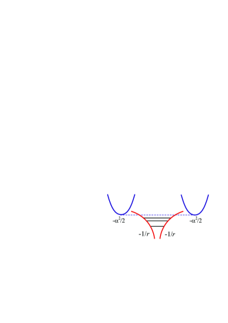
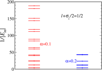
Figure 1: Upper panel: Schematic plot of the discrete spectrum and Rashba-spectrum parabolas. The transition to delocalized states occurs at energies higher than $-\alpha^{2}/2.$ Lower panel: Bound states spectra $E_{m}$ with $l+\sigma_{z}/2=1/2$ at $\alpha=0.1$ and $\alpha=0.2$, demonstrating the absence of the degeneracy with the increase in $m$.

II General formalism

The Hamiltonian describing 2D exciton can be presented in the form ${\mathcal{H}}={\mathcal{H}}_{0}+{\mathcal{H}}_{\mathrm{so}}$. The spin-independent part reads

$${\mathcal{H}}_{0}=\frac{p^{2}}{2\mu}-\frac{e^{2}}{\kappa r},$$ (1)

where $\mathbf{r}=(x,y)$ is the electron position, $\mathbf{p}=-i\hbar{\bm{\nabla}}$ is the momentum, $\mu$ is its mass, $e$ is the charge, and $\kappa$ is the dielectric constant of a host crystal. The SOC has the Rashba form [Bychkov, ], arising in 2D structures as a result of the spatial structural inversion asymmetry:Bychkov ; Fabian

$${\mathcal{H}}_{\mathrm{so}}=\frac{\alpha}{\hbar}\left(p_{x}{\sigma}_{y}-p_{y}{\sigma}_{x}\right),$$ (2)

with $\alpha$ being the coupling constant and $\sigma_{i}$ ($i=x,y,z$) being the corresponding Pauli matrices.

In the presence of spin-orbit coupling (2), the integral of motion corresponding to the total angular momentum becomes $l+{\sigma}_{z}/2,$ where $l$ is the $z-$component of the orbital angular momentum. The Runge-Lenz vector, having the form $\mathbf{r}/r-\left(\left[\mathbf{p},\mathbf{l}\right]-\left[\mathbf{l},\mathbf{p}\right]\right)/2$ in the SOC absence, does not have a conserved counterpart here. The discrete energy spectrum ends at the bottom of the conduction band $-\mu\alpha^{2}/2\hbar^{2}.$ Nevertheless, the number of the localized states is still infinite, see Ref. [Chaplik, ] where the case of a weak attractive potential has been considered. The Hamiltonian (2) brings a new feature such as the anomalous spin-dependent velocity Adams $\mathbf{v}_{\mathrm{so}}\equiv i[H_{\mathrm{so}},\mathbf{r}]/\hbar=\alpha\left({\sigma}_{y},-{\sigma}_{x}\right)/\hbar$. Two other SOC characteristics of interest Fabian are the spin precession with the rate $2p\alpha/\hbar^{2}$ and the corresponding length $l_{\mathrm{so}}=\hbar^{2}/\mu\alpha$, necessary for electron to essentially rotate the spin. Below we set units as $e^{2}/\kappa=\mu=\hbar=1$.

We are seeking the wave function of 2D exciton with SOC in the form of the infinite series (cf. [Grimaldi, ]) over complete set of discrete eigenstates of Hamiltonian ${\mathcal{H}}_{0}$ [Yang, ]:

$${\bm{\psi}}_{l}^{[m]}\left(r,\varphi\right)=e^{il\varphi}\sum_{n=l+1}\left[\begin{array}[]{c}c_{l,n\uparrow}^{[m]}R_{n,l}(r)\\ 0\end{array}\right]+$$ (5)

$$e^{i(l+1)\varphi}\sum_{n=l+2}\left[\begin{array}[]{c}0\\ c_{l,n\downarrow}^{[m]}R_{n,l+1}(r)\end{array}\right].$$ (8)

Here we take into account the conservation of total angular momentum $l+{\sigma}_{z}/2$. Index $m$ enumerates the eigenstates for given $l$ in the ascending energy order. Radial functions $R_{n,l}(r)$ correspond to the eigenstates of the Hamiltonian ${\mathcal{H}}_{0}$ and can be expressed as: Yang

$$R_{n,l}\left(r\right) = N_{n,l}r_{n}^{\left|l\right|}e^{-r_{n}/2}\,_{1}F_{1}\left(-n+\left|l\right|+1,2\left|l\right|+1,r_{n}\right)$$

$$N_{n,l} = \frac{\beta_{n}}{\left(2\left|l\right|\right)!}\left[\frac{\left(n+\left|l\right|-1\right)!}{(2n-1)\left(n-\left|l\right|-1\right)!}\right]^{1/2},$$ (9)

where dimensionless $\beta_{n}={2}/\left(n-1/2\right),$ $r_{n}=r\beta_{n}$ and $l=-(n-1),...,n-1.$ The expansion coefficients are the eigenvectors of the Hamiltonian:

$$\left[\begin{array}[]{cc}\mathcal{H}_{l}^{\uparrow\uparrow}&\mathcal{H}_{l}^{\uparrow\downarrow}\\ \mathcal{H}_{l}^{\downarrow\uparrow}&\mathcal{H}_{l}^{\downarrow\downarrow}\end{array}\right]\left[\begin{array}[]{c}\mathbf{c}_{l,n\uparrow}^{[m]}\\ \mathbf{c}_{l,n\downarrow}^{[m]}\end{array}\right]=E_{m}\left[\begin{array}[]{c}\mathbf{c}_{l,n\uparrow}^{[m]}\\ \mathbf{c}_{l,n\downarrow}^{[m]}\end{array}\right].$$ (10)

The blocks $\mathcal{H}^{\uparrow\uparrow}$ and $\mathcal{H}^{\downarrow\downarrow}$ are diagonal with the elements given by the corresponding eigenenergies $E_{n}=-1/2(n-1/2)^{2}$ for 2D exciton without SOC. The blocks $\mathcal{H}^{\uparrow\downarrow}$ and $\mathcal{H}^{\downarrow\uparrow}$ couple spin-up and spin-down states due to the Rashba interaction. The off-diagonal elements are given by:

$$\mathcal{H}_{l,n_{1},n_{2}}^{\uparrow\downarrow}=\alpha\times$$ (11)

$$\int R_{n_{1},l}(r)\left(\frac{d}{dr}R_{n_{2},l+1}(r)+\frac{l+1}{r}R_{n_{2},l+1}(r)\right)rdr.$$

Note that the off-diagonal elements (11) are usually small since $R_{nl}$ are rapidly oscillating functions.

III Analytical results with semiclassical approach

Although the matrix elements (11) can be evaluated analytically using properties of hypergeometric functions,land3 ; Gradshteyn this calculation is quite cumbersome. Thus, it is instructive to apply the simpler semiclassical approach for this purpose. This approach is valid at large-$l$, which is of interest here since for the Rydberg states with $n\gg 1$, typical values of angular momentum are also large $l\gg 1$. Semiclassical evaluation of matrix elements (11) is also useful as it permits to trace analytically the main matrix elements leading to the level repulsion. After separation of angular and radial variables, the effective Coulomb potential can be rendered as $\widetilde{U}(r)=-1/r+l^{2}/2r^{2},$ and at a given energy $E$, the semiclassical return points with $\widetilde{U}(r)=E$ are given by:

$$r=\frac{l^{2}}{1\pm\sqrt{1+2l^{2}E}}.$$ (12)

For $l^{2}|E|\ll 1,$ the points are $r_{\min}=l^{2}/2$ and $r_{\max}=-1/E,$ respectively. Forces acting on the electron at the return points are $F\left(r_{\min}\right)=-4/l^{4}$ and $F\left(r_{\max}\right)=E^{2}\ll F\left(r_{\min}\right).$ As a result, the non-semiclassical domain near $r_{\max}$ is determined by: $r_{\max}-r\leq E^{-2/3},$ confirming validity of the semiclassical approximation since $r_{\max}\sim 1/E.$

The minimum of $\widetilde{U}(r)$ is achieved at $r_{l}=l^{2}$ with $r_{l+1}-r_{l}=2l+1,$ and $\widetilde{U}(r_{l})=-1/2l^{2}.$ The near-the-minimum oscillation frequencies are given by $\Omega=\sqrt{\widetilde{U}^{\prime\prime}(r_{l})}=1/l^{3}.$ The corresponding oscillator length $\ell=\sqrt{1/\Omega}=l^{3/2}\gg 2l$ implies that the states with orbital momenta $l$ and $l+1$ have a large spatial overlap. Taking into account that $\Omega\ll\left|\widetilde{U}(r_{l})\right|,$ we conclude that these are well-described in terms of harmonic oscillators centered at the points $r_{l}$ or $r_{l+1}$. In this approximation we obtain

$$R_{n,l}(r)=\sqrt{\frac{1}{2\pi r_{l}}}\phi_{n^{[r]}}(y),$$ (13)

where $y=\left(r-r_{l}\right)/l^{3/2}$ and $\phi_{n^{[r]}}(y)$ is the oscillator wavefunction with the radial quantum number $n^{[r]}=n-l-1$. With these functions one can evaluate the integrals in Eq. (11) in semiclassical approach. We begin with corresponding overlap of shifted wavefunction:

$$\int\phi_{n^{[r]}_{1}}(y)\phi_{n^{[r]}_{2}}(y)dy=$$ (14)

$$N_{1}N_{2}e^{-\widetilde{l}^{2}}\int e^{-y^{2}}H_{n^{[r]}_{1}}\left(y+\widetilde{l}\right)H_{n^{[r]}_{2}}\left(y-\widetilde{l}\right)dy$$

with normalization coefficients $N_{1}$ and $N_{2}$ and $\widetilde{l}=1/l^{1/2},$ with $H_{n^{[r]}_{1}}\left(y+\widetilde{l}\right)$ and $H_{n^{[r]}_{2}}\left(y-\widetilde{l}\right)$ being the Hermitian polynomials.land3 ; Gradshteyn

The integration yields Gradshteyn

$$\int e^{-y^{2}}H_{j}\left(y+z_{1}\right)H_{k}\left(y+z_{2}\right)dy=$$ (15)

$$2^{k}\sqrt{\pi}j!z_{2}^{k-j}L_{j}^{k-j}\left(-2z_{1}z_{2}\right),$$

where $L_{j}^{k-j}\left(-2z_{1}z_{2}\right)$ are Laguerre polynomials.land3 ; Gradshteyn In our case $\widetilde{l}^{2}\ll 1$, we can use the limit $L_{j}^{k-j}\left(0\right)=k!/j!\left(k-j\right)!$ to obtain:

$$\int\phi_{n^{[r]}_{1}}(x)\phi_{n^{[r]}_{2}}(x)dx=\sqrt{\frac{2^{n^{[r]}_{2}}{n^{[r]}_{2}!}}{2^{n^{[r]}_{1}}n^{[r]}_{1}!}}\frac{\left(-\widetilde{l}\right)^{n^{[r]}_{2}-n^{[r]}_{1}}}{\sqrt{\left(n^{[r]}_{2}-n^{[r]}_{1}\right)!}}.$$ (16)

Integrals of the type

$$\int R_{n_{1},l}(r)\frac{d}{dr}R_{n_{2},l+1}(r)d^{2}r$$ (17)

can be calculated with Eqs. (13) and (15) using the identity

$$\frac{d}{dy}\phi_{n^{[r]}}(y)=\frac{1}{\sqrt{2}}\left[\sqrt{n^{[r]}}\phi_{n^{[r]}-1}(y)-\sqrt{n^{[r]}+1}\phi_{n^{[r]}+1}(y)\right].$$ (18)

As a result, the $l-$dependence of the SOC matrix element is given by $\sim l^{-\left(n^{[r]}_{2}-n^{[r]}_{1}\right)/2-1}$. Taking into account that the oscillator frequency is $\Omega=l^{-3}$, we obtain that two states are strongly coupled, that is $\left|\mathcal{H}_{l,n_{1},n_{2}}^{\uparrow\downarrow}\right|/\Omega>1$ if $l^{2-\left(n^{[r]}_{2}-n^{[r]}_{1}\right)/2}\geq 1/\alpha$. As a result, statistical distribution of the levels in the corresponding domain is noticeably modified by the spin-orbit coupling.

Within the above semiclassical approach, the strong SOC conditions can be reformulated as $r>1/\alpha$ for the considerable spin rotation and $v\sim\alpha$ for the effect of spin-orbit coupling on the electron velocity. Taking into account that $r_{l}\sim l^{2}$ and $v\sim 1/l$, the second relation can be rewritten as $l>1/\alpha$. This condition coincides with $|\widetilde{U}(r_{l})|<\alpha^{2}.$

IV Numerical results: non-Poissonian spectral statistics

We begin with characterizing the system spectrum. As shown in Fig. 1(lower panel), the infinite degeneracy typical for 2D $U(r)=-1/r$ potential disappears due to the SOC presence, meaning that we observe the level repulsion. Here the state with $m=l+1$ remains nondegenerate while other states produce split doublets with the splitting proportional to $\alpha^{2}$ for the first doublet (since $\mathcal{H}_{l,l+2,l+3}^{\uparrow\downarrow}=0)$ or to $\alpha$ for the states higher in the energy.

To illustrate the relation to possible emergence of chaos, we analyze the statistics of the spectrum in a narrow interval strongly influenced by the SOC as presented in Fig. 2. One can clearly see the distinct deviation from the Poisson distribution. Even though not strong enough to suggest the emergence of quantum chaos, the level distribution shows that the SOC affects the regular character of the motion. In Fig. 2 we show the histograms for the two values of SOC, $\alpha=0.05$ and $\alpha=0.1$, with the $174$ and $73$ energy levels taken from the energy interval $(-2\alpha^{2},-0.51\alpha^{2})$, respectively. Similarly to Refs. [Marchukov, ,Marchukov2, ], here we remove the double degeneracy related to the time-reversal symmetry preserved by the spin-orbit coupling. One can see that for stronger SOC the distribution becomes wider which means stronger energy levels repulsion. To quantify the effect of the level repulsion, we compare the histogram in Fig.2 with that of 2D hydrogen atom at $\alpha=0$, where states are highly degenerate. Taking into account that for large $n$ the interlevel distance $E_{n+1}-E_{n}=1/n^{3}+O\left(1/n^{5}\right)$ and choosing a single histogram interval $s-\Delta_{s}/2<\left(E_{n+1}-E_{n}\right)/\epsilon<s+\Delta_{s}/2,$ where $\epsilon$ is the mean distance between the adjacent levels and $s$ is the corresponding energy bin size, yields the boundaries for the states numbers $n_{\max}=\epsilon^{-1/3}\left(s-\Delta_{s}/2\right)^{-1/3},$ and $n_{\min}=\epsilon^{-1/3}\left(s+\Delta_{s}/2\right)^{-1/3}.$ The number of the states in the interval $\left(n_{\min},n_{\max}\right)$, $\Delta N$ given by $\Delta N=n_{\max}^{2}-n_{\min}^{2}$ yields $\Delta N=2\epsilon^{-2/3}\Delta_{s}/3s^{5/3}$ and we obtain $\Delta N\sim\Delta_{s}s^{-5/3}$ rapidly increasing at small $s$. This is qualitatively different from the results shown in Fig. 2, clearly demonstrating the level repulsion caused by the SOC, which is the necessary condition of the quantum chaos.

In general, three types of statistics are expected to describe systems in terms of the distances between the adjacent energy levels. Poissonian statistics $P_{P}(s)=\exp(-s)$ is expected in the absence of chaos. Two other statistics such as the Gaussian Orthogonal Ensemble $P_{\rm GOE}(s)=\pi/2\times s\exp(-\pi s^{2}/4)$ and the Gaussian Unitary Ensemble $P_{\rm GUE}(s)=32/\pi^{2}\times s^{2}\exp(-4s^{2}/\pi)$ (observed in Ref. [Assmann2016, ]), are expected for different quantum chaos realizations. For these two, the level repulsion should be sufficiently strong to yield $P_{\rm GOE}(0)=P_{\rm GUE}(0)=0.$ Although the distribution in Fig. 2, being a result of the level repulsion, clearly deviates from the Poisson distribution, this repulsion is not sufficiently strong Silva2015 to suppress it at $s\ll 1$.

Note that Refs. [Marchukov, ,Marchukov2, ] examined in detail the spectral properties of another 2D quantum system such as anisotropic harmonic oscillator with SOC in terms of the quantum chaos ensembles. However, the results for the harmonic and Coulomb potentials cannot be compared directly since their eigenstates are qualitatively different in terms of spectrum and wave functions.

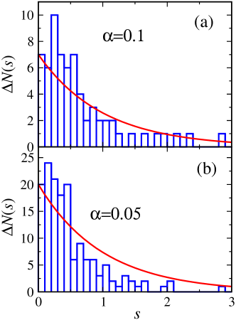
Figure 2: Histogram for eigenenergies statistics in the interval $\left(-2\alpha^{2},-0.51\alpha^{2}\right),$ where the effect of spin-orbit coupling is expected to be strong: (a) $\alpha=0.1$ and (b) $\alpha=0.05.$ Solid red lines correspond to the Poissonian statistics $\sim\exp(-s).$ Note that both panels demonstrate a very similar behavior. In the panel (a) the total energy interval contains 73 energy levels, and in the panel (b) it includes 174 levels.

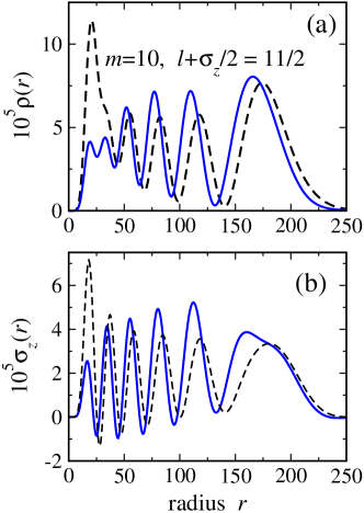
Figure 3: Charge (a) and spin density (b) distributions for given eigenstate at $\alpha=0.1$. For comparison, we present by dashed lines the densities corresponding to correct zeroth-approximation functions, that is $\left(R_{11,5}^{2}+R_{11,6}^{2}\right)/2$ and $\left(R_{11,5}^{2}-R_{11,6}^{2}\right)/2$ for the density and for the $\sigma_{z}-$density, respectively. These functions describe densities in the $\alpha\to 0^{+}$ limit.

The inclusion of SOC term into the 2D exciton Hamiltonian affects not only the spectral properties of the system but observables as well. Consider local observables such as charge and spin densities

$$\sigma_{i,l}^{[m]}\left(r,\varphi\right)=\left({\bm{\psi}}_{l}^{[m]}\left(r,\varphi\right)\right)^{{\dagger}}\sigma_{i}{\bm{\psi}}_{l}^{[m]}\left(r,\varphi\right).$$ (19)

The corresponding integral quantities read

$$\left\langle\sigma_{i}\right\rangle_{l}^{[m]}=\int\sigma_{i,l}^{[m]}\left(r,\varphi\right)d^{2}r.$$ (20)

Here, the charge density is characterized by the identity matrix $\sigma_{0}$. Note that $\langle\sigma_{x}\rangle_{l}^{[m]}=\langle\sigma_{y}\rangle_{l}^{[m]}=0$ due to orthogonality of the wave functions corresponding to different values of $l$ contributing to the spinors. In addition, the in-plane components of the spin have the symmetry $\sigma_{x,l}^{[m]}\left(r,\varphi\right)=\sigma_{l}^{[m]}(r)\cos\varphi$ and $\sigma_{y,l}^{[m]}\left(r,\varphi\right)=\sigma_{l}^{[m]}(r)\sin\varphi,$ respectively. Note that for Eq. (8): $\left\langle\sigma_{z}\right\rangle_{l}^{[m]}=1-2\sum_{n}\left|c_{l,n\downarrow}^{[m]}\right|^{2}<1.$

To illustrate the effect of the SOC on the eigenfunctions, we take a single eigenstate in the semiclassical domain and show corresponding charge and spin densities in Fig. 3. As one can see, the behavior of the densities for finite $\alpha$ and those in the limit $\alpha\to\ 0$ are noticeably different.

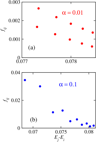
Figure 4: Oscillator strengths for selected transitions with $l_{i}=2,$ $l_{j}=3$ for two different values of spin-orbit coupling, indicated in the panels.

Related quantity, which can be experimentally measured, is the oscillator strength of the optical transition $f_{ij}=\left(E_{j}-E_{i}\right)\left|x_{ij}\right|^{2},$ where $x_{ij}$ is the matrix element of the coordinate $x=r\cos\varphi\equiv r\left(e^{i\varphi}+e^{-i\varphi}\right)/2$ for transitions satisfying the selection rules: $l_{j}=l_{i}\pm\,1$. We obtain for the transition $l_{j}=l_{i}+1$

$$f_{ij}=\sum_{n_{1}=n+1}\sum_{n=l+1}c_{l+1,n_{1}\uparrow}^{[m_{1}]}c_{l,n\uparrow}^{[m]}r_{l\to l+1,n\to n_{1}}+$$

$$\sum_{n_{1}=n+1}\sum_{n=l+2}c_{l+1,n_{1}\downarrow}^{[m_{1}]}c_{l,n\downarrow}^{[m]}{r}_{l+1\rightarrow l+2,n\rightarrow n_{1}},$$ (21)

$${r}_{l+1\rightarrow l+2,n\rightarrow n_{1}}=\int r^{2}R_{n_{1},l+2}(r)R_{n,l+1}(r)dr.$$ (22)

Matrix elements (22) can be calculated semiclassically similarly to Eq. (15). The results of numerical calculations are presented in Fig. 4. At $\alpha=0.01$ the transitions demonstrate clear doublet structure. Although for $\alpha=0.1$ the general structure of the spectrum, shown here up to the endpoint near the $-\alpha^{2}/2,$ and the oscillator strengths distribution becomes less regular, the jigsaw-like pattern described in Ref. [Gutzwiller, ] does not appear here.

To make connections to the experiments, we consider GaAs-based 2D structures that are excellently suited for studies of excitonic spectra.High ; Vishnevsky In this case the characteristic speed $\sqrt{\left|E_{0}\right|/\mu}$ of the electron in the ground state is of the order of $e^{2}/\kappa\sim 10^{7}$ cm/s. Also, the energy of the exciton ground state is of the order of -10 meV. Since the typical structure-dependent values of $\alpha/\hbar$ are of the order 10⁶ cm^-1, the dimensionless $\alpha$ here is about 0.1. Taking into account that the velocity $\sqrt{\left|E_{n}\right|/\mu}$ decreases as $e^{2}/n\kappa$, we conclude that the states prone to chaos are located at $n\sim 10$, corresponding to the present analysis.

We are now in a position to discuss the effects related to the Berry curvature.zhou15 The common 2D systems in this case are monolayers of transition metals dichalcogenides like MX₂ (where M=Mo, W and X=S, Se) as they were used for estimations in Ref. [zhou15, ]. It has been shown experimentally nat14 that exciton binding energy, e.g., a in single layer WS₂ is close to 0.7 eV, which is extremely large as compared to the typical values of 10 meV for conventional semiconductors. In Ref. [zhou15, ], the role of SOC $\alpha$ is played by the quantity $\omega\nabla V$, where $\omega$ is the Berry curvature and $V({\bf r})$ is the screened Coulomb interaction. Denoting $\alpha_{0}\equiv\omega{\bar{V}}/a_{0}$ (where $a_{0}$ is the exciton Bohr radius and ${\bar{V}}$ is the average potential which could be around half of the exciton binding energy), we estimate this quantity to be $\alpha_{0}\approx 0.26$ eV$\rm{\AA}$ for the typical values $\omega\approx 15$ ${\rm\AA}^{2}$ and $a_{0}\approx 20$ $\rm{\AA}.$nat14 ; zhou15 Note that this effective SOC constant $\alpha_{0}$ turns out to be less than that, e.g., for semiconducting perovskite layers $\alpha\approx 1$ eV$\rm{\AA}.$mypccp2018 ; r51 However, the effect of the term $\omega\nabla V$ on the spectra of Rydberg excitons in conventional semiconductor heterostructures can be strongly different due to the material dependence of the Berry $\omega-$parameter and the high spread of the $V-$potential. In general, the above estimations are vulnerable to many factors and primarily to the system and samples type. We postpone the discussion of the Berry curvature influence on chaos in 2D Rydberg excitons for future research.

V Conclusions and outlook

We demonstrated that spin-orbit coupling induces effective level repulsion resulting in a non-singular distribution of the distances between the adjacent energy levels and suggesting a possible crossover to a quantum chaotic regime. Although we did not observe the inherent in strong quantum chaos Gutzwiller qualitative deviation of the levels statistics from the Poissonian one, the observed statistics can be a precursor to emergence of the quantum chaos-related Gaussian Orthogonal or the Unitary ensembles. A possible reason for the observed distribution of the levels is that the density of states here is infinite as the energy approaches $-\alpha^{2}/2,$ and the level repulsion has to counteract this strong divergence. This situation is opposite to more conventional quantum chaotic systems such as trapped cold atoms or those with the orbital motion quantized by a magnetic field, where such a divergence does not occur.

In particular, this result implies that quantization ”suppresses” the manifestations of the classical chaos emerging in two-dimensional excitons due to the Rashba spin-orbit interaction mypccp2018 , meaning that the quantization makes the system more ”ordered” than its classical counterpart. Thus, the quantization of a system demonstrating a classical chaos, may, in general, not generate as vivid chaos manifestations, as observed for its classical motion; and this is one of the main messages of this paper. To trace the origin of this difference, the semiclassical Wentzel-Kramers-Brillouin-like analysis land3 of the quantum problem might be useful for the future studies.

To get more insight into the possible quantum chaotic features of this system, the experimental studies of two-dimensional semiconductor structures with spin-orbit coupled Rydberg excitons are highly desirable. These studies can shed light on the corresponding energy levels statistics. We also note that the studies of quasistationary exciton states with the energies above the $-\alpha^{2}/2$ threshold would be of interest as they can demonstrate other types of statistics in the real part of the eigenenergies.

- (1) M. Aßmann, J. Thewes, D. Fröhlich, and M. Bayer, Nat. Mater. 15, 741 (2016).
- (2) E. A. Ostrovskaya and F. Nori, Nat. Mater. 15, 702 (2016).
- (3) F. Schweiner, J. Main, and G. Wunner, Phys. Rev. E 95, 062205 (2017).
- (4) F. Schweiner, J. Main, and G. Wunner Phys. Rev. Lett. 118, 046401 (2017).
- (5) M. C. Gutzwiller, Chaos in Classical and Quantum Mechanics (Springer-Verlag, New York, 1990).
- (6) L. E. Reichl, The Transition to Chaos. Conservative Classical Systems and Quantum Manifestations, 2nd ed. (Springer-Verlag, New York, 2004).
- (7) F. Haake, Quantum Signatures of Chaos, 3rd ed. (Springer-Verlag, Berlin/Heidelberg, 2010).
- (8) H.-J. Stöckmann, Quantum Chaos: An Introduction (Cambridge University Press, Cambridge, U.K., 1999).
- (9) A. Frisch, M. Mark, K. Aikawa, F. Ferlaino, J. L. Bohn, C. Makrides, A. Petrov and S. Kotochigova, Nature 507, 475 (2014).
- (10) T. Gao, E. Estrecho, K. Y. Bliokh, T. C. H. Liew, M. D. Fraser, S. Brodbeck, M. Kamp, C. Schneider, S. Höfling, Y. Yamamoto, F. Nori, Y. S. Kivshar, A. G. Truscott, R. G. Dall, and E. A. Ostrovskaya, Nature 526, 554 (2015).
- (11) Spin Physics in Semiconductors Springer Series in Solid-State Sciences, Ed. by M. I. Dyakonov, Springer (2008).
- (12) M. V. Durnev and M. M. Glazov, Phys. Rev. B 93, 155409 (2016)
- (13) D. V. Vishnevsky, H. Flayac, A. V. Nalitov, D. D. Solnyshkov, N. A. Gippius, and G. Malpuech, Phys. Rev. Lett. 110, 246404 (2013).
- (14) A. A. High, A. T. Hammack, J. R. Leonard, S. Yang, L. V. Butov, T. Ostatnický, M. Vladimirova, A. V. Kavokin, T. C. H. Liew, K. L. Campman, and A. C. Gossard, Phys. Rev. Lett. 110, 246403 (2013).
- (15) C. Grimaldi, Phys. Rev. B 77, 113308 (2008).
- (16) J. Zhou, Wen-Yu Shan, W. Yao and Di Xiao Phys. Rev. Lett. 115, 166803 (2015).
- (17) D.G.W. Parfitt and M.E. Portnoi, Journ. of Math. Phys. 43, 4681 (2002).
- (18) V.A. Stephanovich and E. Ya. Sherman, Phys. Chem. Chem. Phys. 20, 7836 (2018); ArXiv:1711.08773.
- (19) Yu. A. Bychkov and E.I. Rashba, JETP Lett. 39, 78 (1984).
- (20) I. Žutić, J. Fabian, and S. Das Sarma, Rev. Mod. Phys. 76, 323 (2004).
- (21) A. V. Chaplik and L. I. Magarill, Phys. Rev. Lett. 96, 126402 (2006).
- (22) E. N. Adams and E. I. Blount, J. Phys. Chem. Solids 10, 286 (1959).
- (23) X. L. Yang, S. H. Guo, F. T. Chan, K. W. Wong, and W. Y. Ching, Phys. Rev. A 43, 1186 (1991).
- (24) L. D. Landau and E.M. Lifshitz, Quantum Mechanics - Nonrelativistic Theory. Third Edition. Volume 3 Course of Theoretical Physics, (Pergamon Press, 1976).
- (25) I.S. Gradshteyn and I.M. Ryzhik Table of Integrals, Series, and Products (Academic Press, 2000, Cambridge, MA)
- (26) O.V. Marchukov, A.G. Volosniev, D.V. Fedorov, A.S. Jensen, and N.T. Zinner, Journal of Physics B: Atomic, Mol. and Opt. Phys. 47, 195303 (2014).
- (27) O.V. Marchukov, D.V. Fedorov, A.G. Volosniev, A.S. Jensen, and N.T. Zinner, European Physical Journal D 69, 73 (2015).
- (28) It could be of interest to see if this statistics is a realization of a weak chaos, see R. M. da Silva, C. Manchein, M. W. Beims, and E. G. Altmann, Phys. Rev. E 91, 062907 (2015).
- (29) Z. Ye, T. Cao, K. O’Brien, H. Zhu, X. Yin, Y. Wang, S.G. Louie and X. Zhang Nature (London) 513, 214 (2014).
- (30) M. Kepenekian and J. Even, J. Phys. Chem. Lett, 8, 3362 (2017).