Fast parallel multidimensional FFT using advanced MPI

Abstract

We present a new method for performing global redistributions of multidimensional arrays essential to parallel fast Fourier (or similar) transforms. Traditional methods use standard all-to-all collective communication of contiguous memory buffers, thus necessary requiring local data realignment steps intermixed in-between redistribution and transform steps. Instead, our method takes advantage of subarray datatypes and generalized all-to-all scatter/gather from the MPI-2 standard to communicate discontiguous memory buffers, effectively eliminating the need for local data realignments. Despite generalized all-to-all communication of discontiguous data being generally slower, our proposal economizes in local work. For a range of strong and weak scaling tests, we found the overall performance of our method to be on par and often better than well-established libraries like MPI-FFTW, P3DFFT, and 2DECOMP&FFT. We provide compact routines implemented at the highest possible level using the MPI bindings for the C programming language. These routines apply to any global redistribution, over any two directions of a multidimensional array, decomposed on arbitrary Cartesian processor grids (1D slabs, 2D pencils, or even higher-dimensional decompositions). The high level implementation makes the code easy to read, maintain, and eventually extend. Our approach enables for future speedups from optimizations in the internal datatype handling engines within MPI implementations.

1 Introduction

The Fast Fourier Transform (FFT) remains one of the most significant algorithms across various disciplines in science and society. Applications range from image analysis and signal processing to the solution of partial differential equations through spectral methods. Spectral methods are frequently the method of choice for physicists that aim for the most accurate numerical methods to get representations of physical models as realistic as possible. In particular, FFT-based spectral methods are at the core of all major Direct Numerical Simulation (DNS) codes used in fundamental studies of turbulence and transitional flows. These simulations are pushing the limits of high-performance supercomputers, with computational domains approaching trillions of unknowns. Within such applications, it is crucial to ensure the best possible algorithms for both serial and parallel FFT, which often is the bottleneck of the codes.

It is well known that an FFT on multidimensional data can be performed as a sequence of one-dimensional transforms along each dimension. For example, a multidimensional array of shape $N_{x}\times N_{y}\times N_{z}$ can be Fourier-transformed by first performing $N_{x}\times N_{y}$ serial transforms of length $N_{z}$ along the last axis, followed by $N_{x}\times N_{z}$ transforms of length $N_{y}$ along the middle axis and then finally $N_{y}\times N_{z}$ transforms of length $N_{x}$ along the first axis. However, when the computational domains become too large to fit in the memory locally available within a single compute unit, the domain have to be distributed amongst several, often thousands. In this case, only a small part of the multidimensional array is available on each processor.

It is the job of decomposition algorithms and global redistribution operations to assist in the computation of the multidimensional FFT, by ensuring that array data needed for a serial 1D transform along a given axis is locally available when needed. In the literature, such approaches are often referred as transpose algorithms [1]. An alternative parallel FFT method, which is more intrinsically connected with the FFT algorithm, is the binary exchange (or distributed) method. In this work we will only consider the transpose algorithm, which in general is found to be superior for large problems, and refer to Gupta and Kumar [2] and Foster and Worley [1] for a review of both methods.

At first, multidimensional parallel FFTs based on global redistributions were conducted using slab decompositions, where only one axis of a multidimensional array is distributed. Despite slab decompositions being very efficient, they are unfortunately limited to a rather small number of processors, since that number cannot be larger than $N$, assuming $N=N_{x}=N_{y}=N_{z}$. The next level of parallelism was reached with 2D pencil decompositions [3], where two axes of a multidimensional array were distributed, using one-dimensional subgroups of processors corresponding to rows and columns of a logically two-dimensional processor grid. Pencil decompositions are usually found to be less efficient than slab decompositions, but the number of processors can be as large as $N^{2}$. For such reason, pencil decompositions became the only sensible choice for large-scale simulations using hundreds of thousands of processors.

Several open-source implementations of parallel FFT based on global redistributions are available. For pencil decompositions the P3DFFT [4] and 2DECOMP&FFT [5] are probably the two most commonly used libraries, both being implemented in Fortran 90 and using similar algorithms based on collective all-to-all communication of contiguous arrays followed (or preceded) by a local transpose or remapping operation. Both libraries primarily target three-dimensional arrays and complex-to-complex or real-to-complex/complex-to-real transforms. The PFFT package of Pippig [6] is more general and can be used for even higher-dimensional arrays, using processors grids with more than two dimensions. PFFT is built on top of FFTW [7], which comes with its own slab implementation. However, instead of using FFTW’s built-in slab implementation, PFFT makes use of FFTW’s global transpose routines to implement the 2D (or even higher dimensional) pencil method. Other known parallel FFT libraries are OpenFFT [8], which also admits higher ($>3$) dimensional transforms, AccFFT [9], which utilizes both CPUs and GPUs, the parallel FFT subroutine library of Plimpton [10], FFTW++ [11], which implements both binary exchange and transpose algorithms, and mpiFFT4py [12], which provides a high-level Python interface based on MPI for Python [13, 14].

In this paper we suggest a completely generic, black-box, global redistribution method, based on the generalised all-to-all (MPI_ALLTOALLW) scatter/gather and subarray datatype facilities available in the Message Passing Interface (MPI) standard [15]. To the best of our knowledge this approach has not been explored much in the literature. Derived datatypes were used previously for a slab decomposition by Hoefler and Gottlieb [16], where the local transposes used by regular parallel MPI implementations were described as part of the derived datatype, and speedup over traditional algorithms was demonstrated for some, but not all showcases. The Warp [17] particle-in-cell code is using MPI_ALLTOALLW with derived datatypes for global redistributions, but only for 3D arrays and power-of-two number of processors.

It is in the spirit of extreme-scale architecture design to restructure algorithms to allow taking the rearrangement of data off the critical path of the CPU and into the memory subsystem or the network, provided that the supporting hardware and software of those layers can accommodate. The global redistribution method described in this paper embraces such a paradigm shift, as it eliminates the need for any local remappings. Furthermore, it is applicable to arrays of arbitrary dimensions, decomposed on Cartesian processor grids that are also of arbitrary dimensionality. As in previous parallel (transpose) FFT implementations we assume that there is a serial FFT code already available, and discuss only the parallel decomposition and collective communication required to utilise such a serial code most efficiently in parallel. To this end we introduce some necessary theory and notation on discrete Fourier transforms in Sec 2. In Sec 3, some existing FFT transpose methods are discussed before introducing our new global redistribution method. In Sec 4, we compare scaling of the new method with other well-known parallel FFTs libraries on a Cray XC40 supercomputer. Finally, conclusions are drawn in Sec 5.

2 Sequential FFTs of multidimensional arrays

The discrete Fourier transform (DFT) takes a sequence of complex numbers $u_{0},u_{1},\ldots,u_{N-1}$ and transforms them into another sequence of complex numbers $\hat{u}_{0},\hat{u}_{1},\ldots,\hat{u}_{N-1}$. Forward and backward transforms can be defined, respectively, as

$$\hat{u}_{k} =\frac{1}{N}\sum_{j=0}^{N-1}{u}_{j}e^{-ikx_{j}}\quad k=0,1,\ldots,N-1,$$ (1)

$$u_{j} =\sum_{k=0}^{N-1}\hat{u}_{k}e^{ikx_{j}}\quad j=0,1,\ldots,N-1,$$ (2)

where $i$ is the imaginary unit, $x_{j}=2\pi j/N$, and simplifications are possible if either sequence is real. An alternative and more compact notation is

$$\boldsymbol{\hat{u}} =\mathcal{F}(\boldsymbol{u}),$$ (3)

$$\boldsymbol{u} =\mathcal{F}^{-1}(\boldsymbol{\hat{u}}),$$ (4)

where $\boldsymbol{u}=\{u_{j}\}_{j=0}^{N-1}$, $\boldsymbol{\hat{u}}=\{\hat{u}_{k}\}_{k=0}^{N-1}$ and $\boldsymbol{u}=\mathcal{F}^{-1}(\mathcal{F}(\boldsymbol{u}))$.

The forward and backward DFTs are usually computed using a fast Fourier transform (FFT) algorithm. In this work we will assume that there exist high-performance, serial (single-process, maybe multi-threaded) FFT routines to compute these one-dimensional forward and backward DFTs. These routines are widely available from, e.g., FFTW [7], FFTPACK [18], IBM ESSL [19], or Intel MKL [20].

In many applications numerical data are arranged in multidimensional arrays. We denote a $d$-dimensional array as $u_{j_{0},j_{1},\ldots,j_{d-1}}$, where there are $d$ index sets $j_{m}=0,1,\ldots,N_{m}-1$, $m\in 0,1,\ldots,d-1$, with $N_{m}=|j_{m}|$ being the length of $j_{m}$. A forward $d$-dimensional DFT on the $d$-dimensional array ${u}_{j_{0},j_{1},\ldots,j_{d-1}}$ will then be computed as

$$\hat{u}_{k_{0},k_{1},\ldots,k_{d-1}}=\sum_{j_{0}=0}^{N_{0}-1}\left(\frac{\omega_{0}^{k_{0}j_{0}}}{N_{0}}\sum_{j_{1}=0}^{N_{1}-1}\left(\frac{\omega_{1}^{k_{1}j_{1}}}{N_{1}}\cdots\sum_{j_{d-1}=0}^{N_{d-1}-1}\frac{\omega_{{d-1}}^{k_{d-1}j_{d-1}}}{N_{d-1}}{u}_{j_{0},j_{1},\ldots,j_{d-1}}\right)\right),$$ (5)

where $\omega_{j}=e^{-2\pi i/N_{j}}$. Note that for a transformed axis $m$ we use the index set $k_{m}=0,1,\ldots N_{m}-1$ instead of $j_{m}$, and (5) is executed over all these output indices. As such, we see in (5) that the array $\hat{u}_{k_{0},k_{1},\ldots,k_{d-1}}$ has been transformed along all of its axes. Note that a hat notation, $\hat{u}$, is used exclusively for a fully transformed array, i.e., the output of a complete forward FFT over all axes.

We can simplify Eq. (5) using the notation

$$\hat{u}_{k_{0},k_{1},\ldots,k_{d-1}}=\mathcal{F}_{0}\left(\mathcal{F}_{1}\left(\cdots\mathcal{F}_{d-1}({u}_{j_{0},j_{1},\ldots,j_{d-1}})\right)\right),$$ (6)

where $\mathcal{F}_{i}(\cdot)$ represents a partial transform, i.e., a one-dimensional DFT along axis $i$, for all other index sets unchanged

$$\tilde{u}_{j_{0},\ldots,k_{i},\ldots,j_{d-1}}=\mathcal{F}_{i}(u_{j_{0},\ldots,j_{i},\ldots,j_{d-1}}).$$ (7)

Note that this represents exactly $1/N_{i}\prod_{m=0}^{d-1}N_{m}$ one-dimensional transforms of length $N_{i}$. Also note that here, and for the rest of this paper, tilde notation, $\tilde{u}$, is used to represent an array that is only partially transformed, i.e., transformed along some, but not all, of its axes.

From Eq. (6) it is evident that the DFTs are computed in sequence, one axis of the multidimensional array at a time. A backward $d$-dimensional DFT is executed in the opposite order

$${u}_{j_{0},j_{1},\ldots,j_{d-1}}=\mathcal{F}^{-1}_{d-1}\left(\cdots\mathcal{F}^{-1}_{1}\left(\mathcal{F}^{-1}_{0}(\hat{u}_{k_{0},k_{1},\ldots,k_{d-1}})\right)\right).$$ (8)

Moving from one to several dimensions, the data arrays quickly grow in size, and it becomes necessary to distribute the arrays across several processors within distributed-memory computing architectures. Since the multidimensional FFTs are computed in sequence, one axis at a time, we need only ensure that the whole length of the array along that one axis is available on each single processor when it is up for transformation. Making this happen is the job of global array redistribution procedures, using parallel decompositions and communication as discussed briefly in the introduction, and in sections to come.

3 Parallel FFTs of multidimensional arrays

Consider a $d$-dimensional array $u_{j_{0},j_{1},\ldots,j_{d-1}}$ and pick any one of the index sets $j_{m}=0,1,\ldots,N_{m}-1$, $m\in 0,1,\ldots,d-1$. This index set can be partitioned (and corresponding array entries mapped) into an ordered group of processes $P$ of size $|P|$ with process identifiers $p=0,1,\ldots,|P|-1$. Regardless of how it is partitioned, we denote an index set $j_{m}$ distributed into a process group $P$ as $j_{m}/P$. As such, a $d$-dimensional array that is distributed in its first axis by processor group $P$ will be denoted as $u_{j_{0}/P,j_{1},\ldots,j_{d-1}}$. Note that here and throughout this paper we assume that arrays are in C-style row-major order. For Fortran-style column-major order, it would be natural to distribute the last index set $j_{d-1}$ rather than $j_{0}$.

3.1 Balanced block-contiguous decompositions

There are many different ways of distributing the index set $j_{m}$ on a process group $P$. From the many choices available, we restrict our discussion to block-contiguous decompositions. Such decompositions are fully defined from the global index set length $N_{m}=|j_{m}|$, the number of processes $M=|P|$, and local (that is, within each processor) index set lengths. We denote these local index set lengths of $j_{m}$ as $N_{m}/P$, they correspond to a sequence $\{(N_{m}/P)_{p}\}_{p=0}^{M-1}$. For simplicity, and only in this section, we will use the notation $n_{p}=(N_{m}/P)_{p}$ to refer to the local length corresponding to the $p$-th process. Within the obvious restriction $\sum_{p}n_{p}=N_{m}$, the values $n_{p}$ are otherwise arbitrary. In practice, it is useful to compute and store the start index $s_{p}$ corresponding to each process with the recursion $s_{0}=0$, $s_{k}=s_{k-1}+n_{k-1}$, $k=1,2,\ldots,M-1$.

A balanced block-contiguous decomposition of a sequence of $N_{m}$ elements in $M$ parts $p=0,1,\ldots,M-1$ is given by the simple formula

$$n_{p}=\begin{cases}q+1&\text{if }r>p\\ q&\text{otherwise}\end{cases},\text{ with }q=\left\lfloor\frac{N_{m}}{M}\right\rfloor\text{ and }r=N_{m}\bmod M.$$ (9)

Alg. 1 shows pseudocode using Eq. (9) to compute the local lengths $n_{p}$ along with an explicit, non-recursive expression for the start indices $s_{p}$. Executing the call $n_{p},s_{p}\leftarrow\text{{Decompose}}(|j_{m}|,|P|,p)$ implicitly defines an subset $\{s_{p},\ldots,s_{p}+n_{p}-1\}$ of $j_{m}$ corresponding to the $p$-th process in group $P$. Although admittedly trivial, for the sake of completeness we present in Listing 1 a concrete and concise implementation in the C programming language. For the rest of this paper we trade generality for simplicity and restrict our discussion to balanced block-contiguous decompositions as defined in Eq. (9). Other pseudocodes and listings to be presented later are greatly simplified, as the various $n_{p}$, $s_{p}$ values can be computed with Alg. 1 on the fly and as needed rather than having to store and pass them around function calls.

Algorithm 1 Balanced block-contiguous decomposition

1:function Decompose($N,M,p$)

2:input $N$ : integer $\triangleright$ total number of elements, $N\geq 0$

3:input $M$ : integer $\triangleright$ number of parts, $M>0$

4:input $p$ : integer $\triangleright$ part index, $0\leq p<M$

5:output $n$ : integer $\triangleright$ number of elements in $p$-th part

6:output $s$ : integer $\triangleright$ start index of $p$-th part

7:     $q\leftarrow\lfloor N/M\rfloor$

8:     $r\leftarrow N\bmod M$

9:     if $r>p$ then

10:         $n\leftarrow q+1$

11:         $s\leftarrow n\cdot p$

12:     else

13:         $n\leftarrow q$

14:         $s\leftarrow n\cdot p+r$

15:     end if

16:     return $n,s$

17:end function

Listing 1: Balanced block-contiguous decomposition

⬇

1#define min(x, y) (((x) < (y)) ? (x) : (y))

2void decompose(int N, int M, int p, int *n, int *s)

3{

4 int q = N / M;

5 int r = N % M;

6 *n = q + (r > p);

7 *s = q * p + min(r, p);

8}

3.2 Global redistributions

We can perform a serial FFT on any index set of a multidimensional array that is not distributed. For example, for the array ${u}_{j_{0}/P,j_{1},\ldots,j_{d-1}}$, we can perform a partial transform over all but the first axis as

$$\tilde{u}_{j_{0}/P,k_{1},\ldots,k_{d-1}}=\mathcal{F}_{1}\left(\mathcal{F}_{2}\left(\cdots\mathcal{F}_{d-1}({u}_{j_{0}/P,j_{1},\ldots,j_{d-1}})\right)\right).$$ (10)

However, we cannot perform the transform over the first axis, because only a part of the global array is available locally on each process. It is the job of global redistribution (or transpose) operations to ensure that data within a distributed array is realigned such that a distributed axis becomes locally available in full for all processes in the group. We denote a global redistribution operation from alignment in axis $v$ to alignment in axis $w$ performed within a process group $P$ as

$$u_{\ldots,j_{w},\ldots,j_{v}/P,\ldots}\xleftarrow[P]{v\rightarrow w}u_{\ldots,j_{w}/P,\ldots,j_{v},\ldots}.$$ (11)

Note that axes other than $v$ and $w$ are not involved in the redistribution operation and thus they are not altered by the exchange.

The global redistribution operation brings us to the main novelty of this paper. All known parallel FFT libraries perform global redistributions in two steps (not necessarily in this order):

• Contiguous data communication using collective all-to-all operations.

• Local data rearrangements or transpose operations, also referred as remappings.

Both steps are known to be computationally expensive. The first step involves communicating large amounts of data among processes within the group in an all-to-all fashion. The second step involves non-contiguous memory accesses and copies, which is heavily affected by cache capacity and memory bandwidth of current computing architectures.

In this work, we suggest a global redistribution method that eliminates the need for any local remappings or transposes. To explain how our method works, and how it differs from other methods, we discuss first in Sec. 3.3.1 a traditional implementation of parallel FFTs with slab decomposition using local remappings and all-to-all communication of contiguous memory buffers. Afterwards, in Sec 3.3.2, we show how the slab decomposition can be implemented without local remappings using subarray datatypes and generalized all-to-all communication. We will then, in Sec 3.4, briefly describe multidimensional Cartesian process topologies, that are to be utilized in Secs. 3.5 and 3.6, where the approach will be shown to extend trivially to the 2D pencil method and even higher-dimensional processor grids.

3.3 Slab decomposition

With the notation introduced previously, a parallel FFT on a multidimensional array $u_{j_{0},j_{1},\ldots,j_{d-1}}$, that is initially distributed in a processor group $P$ in the first index set $j_{0}$, can be performed in three steps:

$$\tilde{u}_{j_{0}/P,k_{1},\ldots,k_{d-1}} =\mathcal{F}_{1}\left(\mathcal{F}_{2}\left(\ldots\mathcal{F}_{d-1}(u_{j_{0}/P,j_{1},\ldots,j_{d-1}})\right)\right),$$ (12)

$$\tilde{u}_{j_{0},k_{1}/P,\ldots,k_{d-1}} \xleftarrow[P]{1\rightarrow 0}\tilde{u}_{j_{0}/P,k_{1},\ldots,k_{d-1}},$$ (13)

$$\hat{u}_{k_{0},k_{1}/P,\ldots,k_{d-1}} =\mathcal{F}_{0}(\tilde{u}_{j_{0},k_{1}/P,\ldots,k_{d-1}}).$$ (14)

These steps correspond to a traditional parallel FFT with slab decomposition, as illustrated in Fig. 1 for a three-dimensional array distributed in a group of four processes. We are interested in the global redistribution in the second step, that is usually accomplished with a local remapping followed by a collective all-to-all communication.

3.3.1 Traditional global redistribution method

For a three-dimensional array $\tilde{u}_{j_{0}/P,k_{1},k_{2}}$ (see 13), we can illustrate a global redistribution based on MPI_ALLTOALL on a projected $xy$-plane, since the third index set $k_{2}$ is not affected by the exchange. Fig. 2 is an illustration of Fig. 1 as seen along the $z$-axis, and with the local arrays divided into chunks (or subarrays), four chunks for each slab since there are four processes. Each of the chunks within a process has to be communicated with the other processes. The chunks are labelled with processor number first, and then chunk number. Now, to be able to perform an all-to-all communication the local arrays as seen in Fig. 2(a) need to be packed in a contiguous array such that the chunk going out to rank 0 comes first in memory, then the chunk that goes out to rank 1, and so on. In other words, the local arrays must be remapped to an $x$-alignment with shape $(N_{0},N_{1}/P,N_{2})$, as seen in Fig. 2(b) . This operation is usually referred as a transpose, or permutation, and it is local to each processor. Assuming here for simplicity that $N_{0}$ and $N_{1}$ are divisible by $|P|$, the local transpose operation on the $(N_{0}/P,N_{1},N_{2})$-shaped array can be performed as follows (see Fig 1 of [22])

$$(N_{0}/P,P,N_{1}/P,N_{2}) \xleftarrow{\text{Reshape}}(N_{0}/P,N_{1},N_{2})$$ (15)

$$(P,N_{0}/P,N_{1}/P,N_{2}) \xleftarrow{\text{Swap axes }0\leftrightarrow 1}(N_{0}/P,P,N_{1}/P,N_{2})$$ (16)

$$(N_{0},N_{1}/P,N_{2}) \xleftarrow{\text{Reshape}}(P,N_{0}/P,N_{1}/P,N_{2})$$ (17)

Note that the first and last operations merely represent changes of strides and index sets, and the cost is next to nothing. The transpose operation (16), that swaps the first two axes, is the costly part. After transposing the local arrays to the shapes seen in Fig. 2(b), the datachunks that are to be communicated are contiguous in memory and we may now simply call a collective all-to-all, where the communication pattern is illustrated with bidirectional arrows in Fig. 2(b). The resulting arrays are as shown in Fig. 2(c).

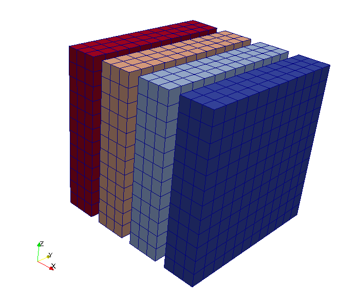
(a) Global array distributed in the $x$-direction.

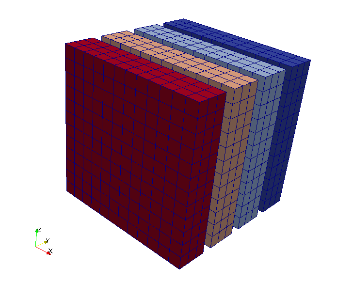
(b) Global array distributed in the $y$-direction.

Figure 1: Slab decomposition. Colours represent CPU rank. Red, orange, light blue and dark blue represent CPUs 0, 1, 2, and 3 respectively.

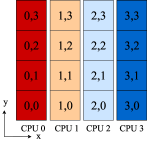
(a) Original array.

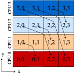
(b) After local transpose.

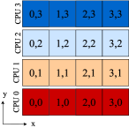
(c) After Alltoall.

Figure 2: Illustration of the slab decomposition. In (a) we see the original global array from Fig 1(a) projected on the $xy$-plane. Each slab is divided into 4 smaller chunks that are to be communicated with the other processors and each chunk is identified with a pair of integer labels. In (b) we see the layout for slabs and chunks after performing a local transpose to align data in $x$-direction. Bidirectional arrows represent a subsequent all-to-all exchange among processors. In (c) we see the layout of the final global array after redistribution. Note that the relative position (within the global array) of each chunk in (a) is preserved in (c), however most chunks have migrated to a different processor.

Note that there are several different ways of performing a global redistribution, and if the global array sizes are not divisible by $|P|$, then the local transpose operation is more complex, and MPI_ALLTOALLV must be used in place of MPI_ALLTOALL. FFTW provides three global redistribution (termed global transpose by FFTW) algorithms, where it is possible to choose a different stride on the output and input arrays, and to combine this with serial FFTs on non-contiguous data. Considering the 3D data in this section, the action of FFTWs global redistribution (that includes all-to-all or similar communication) is then either one of

$$(N_{0},N_{1}/P,N_{2}) \xleftarrow{\text{Regular}}(N_{0}/P,N_{1},N_{2}),$$ (18)

$$(N_{1}/P,N_{0},N_{2}) \xleftarrow{\text{Transposed out}}(N_{0}/P,N_{1},N_{2}).$$ (19)

For FFTW the transposed out option is the fastest, since the regular algorithm is using the transposed out algorithm followed by a global redistribution. FFTW provides an interface that allows for simultaneous planning of local array transpositions and serial FFTs in one single step. PFFT takes advantage of these routines provided in FFTW and performs planning for both the global redistribution and the serial FFTs stages. The choice of making the axes of output arrays transposed in reference to the input is made for efficiency, but naturally it adds a level of complexity, and it is left to the user to make sure that array operations on output arrays take this ordering into consideration. This added complexity is also present in PFFT and P3DFFT, these libraries have options to output arrays with either regular or transposed alignment. The new global redistribution method, to be described in the next subsection, does not transpose the axes of input or output arrays.

3.3.2 A new global redistribution method

As discussed in Sec. 3.3.1, global redistributions for slab decompositions require two steps: i) a local remapping or transpose to rearrange array data in contiguous memory buffers and ii) collective all-to-all communication with these contiguous memory buffers. In the following we describe how the same outcome can be achieved in a single collective communication step. The approach is straightforward if one relies on two slightly advanced features introduced in the MPI-2.0 version of the standard more than 20 years ago. These features allow for collective all-to-all communication of discontiguous memory buffers described through derived datatypes, effectively eliminating the need for any local remapping steps to ensure contiguity.

Overall, our approach takes advantage of the following MPI routines:

• MPI_TYPE_CREATE_SUBARRAY [15, p. 94]. This routine constructs MPI datatypes describing an arbitrary non-strided slice of a dense multidimensional array. Subarray datatypes are routinely used in MPI-based codes and libraries to perform parallel MPI I/O of distributed dense arrays, see [23, p. 207–208] for an executive example. A practical use of subarray datatypes and MPI I/O can be found in PETSc, these features are used in the implementation of of parallel I/O for applications involving structured grids.

• MPI_ALLTOALLW [15, p. 172]. This routine is a generalized all-to-all scatter/gather collective communication operation allowing the specification of send and receive buffers with different datatypes, counts, and displacements for each process within an MPI communicator. To the best of our knowledge, this routine has not been widely used. A practical application we are aware of can be found in PETSc, where MPI_ALLTOALLW is used to implement scatter/gather operations on distributed vectors.

The use of these two routines can be illustrated with reference to Fig. 1 and Fig. 2. First, MPI_TYPE_CREATE_SUBARRAY is used to construct subarray datatypes corresponding to the various array chuncks in Fig. 2(a) and Fig. 2(c). Afterwards, MPI_ALLTOALLW is fed with these datatypes to perform the all-to-all exchange of array data from the layout in Fig. 1(a) to the layout in Fig. 1(b). Thus, there is no need of the intermediate remapping step depicted in Fig. 2(b).

Alg. 2 and Alg. 3 show pseudocode implementing the new global redistribution method, while Listing 2 and Listing 3 present corresponding implementations in the C programming language. Note that these codes have no limitations on the dimensionality or arrays.

Algorithm 2 Subarray datatypes

1:function SubArray($T,N,v,M$)

2:input $T$ : datatype $\triangleright$ elementary datatype descriptor

3:input $N$ : sequence $\triangleright$ local sizes of a $d$-dimensional array

4:input $v$ : integer $\triangleright$ axis to partition, $0\leq v<d$

5:input $M$ : integer $\triangleright$ number of parts, $M>0$

6:output $S$ : sequence $\triangleright$ subarray datatype descriptors

7:     $d\leftarrow\mathbf{len}~{}N$

8:     for $i\leftarrow 0,d-1$ do

9:         $n(i)\leftarrow N(i)$

10:         $s(i)\leftarrow 0$

11:     end for

12:     for $p\leftarrow 0,M-1$ do

13:         $n(v),\,s(v)\leftarrow$ Decompose($N(v),M,p$)

14:         $S(p)\leftarrow$ CreateSubArray($T,N,n,s$)

15:     end for

16:     return $S$

17:end function

Listing 2: Subarray datatypes

⬇

1void subarray(MPI_Datatype datatype,

2 int ndims,

3 int sizes[ndims],

4 int axis,

5 int nparts,

6 MPI_Datatype subarrays[nparts])

7{

8 int subsizes[ndims], substarts[ndims], n, s;

9 for (int i = 0; i < ndims; i++)

10 { subsizes[i] = sizes[i]; substarts[i] = 0; }

11 for (int p = 0; p < nparts; p++) {

12 decompose(sizes[axis], nparts, p, &n, &s);

13 subsizes[axis] = n; substarts[axis] = s;

14 MPI_Type_create_subarray(

15 ndims, sizes, subsizes, substarts,

16 MPI_ORDER_C, datatype, &subarrays[p]);

17 MPI_Type_commit(&subarrays[p]);

18 }

19}

Algorithm 3 Exchange of arrays

1:procedure Exchange($P,A,v,B,w$)

2:input $P$ : communicator $\triangleright$ group of communicating processes

3:input $A$ : array $\triangleright$ local array of elementary datatype $T$

4:input $v$ : integer $\triangleright$ axis of alignment for $A$

5:output $B$ : array $\triangleright$ local array of elementary datatype $T$

6:input $w$ : integer $\triangleright$ axis of alignment for $B$, $w\neq v$

7:     $T\leftarrow$ Type($A$)$\triangleright$ elementary datatype of array $A$

8:     $N_{A}\leftarrow$ Shape($A$)$\triangleright$ sequence with sizes of array $A$

9:     $N_{B}\leftarrow$ Shape($B$)$\triangleright$ sequence with sizes of array $B$

10:     $M\leftarrow$ Size($P$)$\triangleright$ number of processes in group

11:     $S_{A}\leftarrow$ SubArray($T,N_{A},v,M$)$\triangleright$ sequence of datatypes for sending

12:     $S_{B}\leftarrow$ SubArray($T,N_{B},w,M$)$\triangleright$ sequence of datatypes for receiving

13:     AllToAllW($P,A,S_{A},B,S_{B}$)$\triangleright$ generalized all-to-all scatter/gather

14:end procedure

Listing 3: Exchange of arrays

⬇

1void exchange(MPI_Comm comm,

2 MPI_Datatype datatype,

3 int ndims,

4 int sizesA[ndims],

5 void *arrayA,

6 int axisA,

7 int sizesB[ndims],

8 void *arrayB,

9 int axisB)

10{

11 int nparts;

12 MPI_Comm_size(comm, &nparts);

13 MPI_Datatype subarraysA[nparts], subarraysB[nparts];

14 subarray(datatype, ndims, sizesA, axisA, nparts, subarraysA);

15 subarray(datatype, ndims, sizesB, axisB, nparts, subarraysB);

16 int counts[nparts], displs[nparts];

17 for (int p = 0; p < nparts; p++)

18 { counts[p] = 1; displs[p] = 0; }

19 MPI_Alltoallw(arrayA, counts, displs, subarraysA,

20 arrayB, counts, displs, subarraysB, comm);

21 for (int p = 0; p < nparts; p++) {

22 MPI_Type_free(&subarraysA[p]);

23 MPI_Type_free(&subarraysB[p]);

24 }

25}

In Alg. 2, the Decompose() function from Alg. 1 handles decompositions in $M$ parts by computing the local lenghts and starting indices required to define the output subarray datatype sequence $S=\{S_{p}\}_{p=0}^{M-1}$. Each subarray datatype entry $S_{p}$ is created with calls to CreateSubArray(), which represents an invocation to MPI_TYPE_CREATE_SUBARRAY. The output datatype sequence $S$ effectively encodes a block-contiguous, one-dimensional partition in $M$ chunks along a non-distributed axis of alignment $v$ for any $d$-dimensional local array of elementary datatype $T$.

In Alg. 3, the SubArray() function from Alg. 2 is invoked to create subarray datatypes sequences $S_{A}$ and $S_{B}$ using the shapes of the local input and output arrays $A$ and $B$ and their respective axes of alignment $v$ and $w$. Recalling Fig. 1, $A$ corresponds to source arrays with sizes $(N_{0}/P,N_{1},N_{2})$ as in Fig. 1(a), whereas $B$ corresponds to destination arrays with sizes $(N_{0},N_{1}/P,N_{2})$ as in Fig. 1(b). The subarray datatype sequences $S_{A}$ and $S_{B}$ correspond to the various chunks depicted in Fig. 2(a) and Fig. 2(c), respectively. Finally, the call to AllToAllW() represents an invocation of MPI_ALLTOALLW to perform collective all-to-all exchange or array data. Evidently, there is no need for local transposes or remappings.

Executing the call $\text{{Exchange}}(P,A,v,B,w)$ amounts to a global redistribution within a process group $P$ from array $A$ in $v$-alignment to array $B$ in $w$-alignment, and in the previous notation it corresponds to

$$B_{\ldots,j_{w},\ldots,j_{v}/P,\ldots}\xleftarrow[P]{v\rightarrow w}{A}_{\ldots,j_{w}/P,\ldots,j_{v},\ldots}.$$ (20)

Note that the subarray datatypes created in Alg. 3 and Listing 3 do not hold any array data in their own; they are merely descriptors encoding array slicing operations. The internal datatype handling engine within an MPI implementation is able to decode the slicing information to complete the all-to-all communication with the expected outcome, thus ensuring the black-box nature of our approach. Consequently, rather than creating and destroying datatypes as done in Listing 3, a production code should use Listing 2 in a setup phase to create subarray datatypes, and reuse them as many times as needed to perform data redistributions in one-line calls to MPI_ALLTOALLW.

3.4 Cartesian process topologies

Slab decompositions, as described in Sec. 3.3, are one-dimensional decompositions. Despite being very efficient in the context of parallel FFTs, one-dimensional decompositions limit the amount of parallelism that can be thrown at a problem. Recalling the redistribution step in Eq. (13), we necessarily require $|P|\leq\text{min}(|j_{0}|,|k_{1}|)$. The next level of parallelism is reached with multi-dimensional decompositions, to be presented shortly in Sec. 3.5. As a necessary prelude, this section will discuss multi-dimensional Cartesian processor grids.

Consider the rearrangement of a process group $P$ as a logically two-dimensional Cartesian grid of $M_{0}\times M_{1}$ processes such that $|P|=M_{0}\cdot M_{1}$. For each process in $|P|$ with identifier $p=0,1,\ldots,|P|-1$ we assign a two-tuple of process coordinates $(p_{0},p_{1})$ with $p_{i}=0,1,\ldots,M_{i}-1$ corresponding to each direction $i=0,1$. Such assignment of coordinates induces a partitioning of the Cartesian topology in one-dimensional subgroups corresponding to each direction. In the first direction, we obtain $M_{1}$ subgroups collectively denoted $P_{0}$, each with $|P_{0}|=M_{0}$ processes with identifiers $p_{0}$. Similarly, in the second direction, we obtain $M_{0}$ subgroups $P_{1}$ collectively denoted $P_{1}$, each with $|P_{1}|=M_{1}$ processes with identifiers $p_{1}$. Fig. 3 depicts these steps for a group of $12$ processes arranged as a two-dimensional grid of ${3}\times{4}$ processes. The generalization to higher dimensions is straightforward.

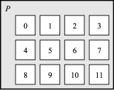
(a) A process group $P$ with 12 processes.

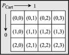
(b) Cartesian grid with ${3}\times{4}$ processes.

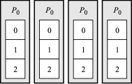
(c) Subgroups $P_{0}$ in first direction.

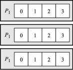
(d) Subgroups $P_{1}$ in second direction.

Figure 3: Two-dimensional Cartesian process grid and one-dimensional process subgroups corresponding to each direction.

The MPI standard provides many facilities for managing Cartesian processor grids. The utility routine MPI_DIMS_CREATE [15, p. 293] can be used to compute a balanced distribution of processes among a given number of dimensions. The routine MPI_CART_CREATE [15, p. 292] constructs process groups with attached Cartesian topology. Finally, the routine MPI_CART_SUB [15, p. 311] partitions a Cartesian topology in lower-dimensional subgroups. These routines are combined in Listing 4 to define a Cartesian topology and obtain the partitions corresponding to each direction. Note that this code can handle processor grids of any dimensionality.

Listing 4: One-dimensional subgroups of a Cartesian process grid

⬇

1void subcomm(MPI_Comm comm,

2 int ndims,

3 MPI_Comm subcomms[ndims])

4{

5 MPI_Comm comm_cart;

6 int nprocs, dims[ndims], periods[ndims], remdims[ndims];

7 for (int i = 0; i < ndims; i++)

8 { dims[i] = periods[i] = remdims[i] = 0; }

9 MPI_Comm_size(comm, &nprocs);

10 MPI_Dims_create(nprocs, ndims, dims);

11 MPI_Cart_create(comm, ndims, dims, periods, 1, &comm_cart);

12 for (int i = 0; i < ndims; i++) {

13 remdims[i] = 1;

14 MPI_Cart_sub(comm_cart, remdims, &subcomms[i]);

15 remdims[i] = 0;

16 }

17 MPI_Comm_free(&comm_cart);

18}

3.5 Pencil decomposition

A pencil decomposition makes use of two subgroups of processors, and distributes two index sets simultaneously in a multidimensional array. A parallel FFT on a three-dimensional array that is initially distributed with processor groups $P_{0}$ and $P_{1}$, can be performed in five steps:

$$\tilde{u}_{j_{0}/P_{0},j_{1}/P_{1},k_{2}} =\mathcal{F}_{2}\left(u_{j_{0}/P_{0},j_{1}/P_{1},j_{2}}\right),$$ (21)

$$\tilde{u}_{j_{0}/P_{0},j_{1},k_{2}/P_{1}} \xleftarrow[P_{1}]{2\rightarrow 1}\tilde{u}_{j_{0}/P_{0},j_{1}/P_{1},k_{2}},$$ (22)

$$\tilde{u}_{j_{0}/P_{0},k_{1},k_{2}/P_{1}} =\mathcal{F}_{1}(\tilde{u}_{j_{0}/P_{0},j_{1},k_{2}/P_{1}}),$$ (23)

$$\tilde{u}_{j_{0},k_{1}/P_{0},k_{2}/P_{1}} \xleftarrow[P_{0}]{1\rightarrow 0}\tilde{u}_{j_{0}/P_{0},k_{1},k_{2}/P_{1}},$$ (24)

$$\hat{u}_{k_{0},k_{1}/P_{0},k_{2}/P_{1}} =\mathcal{F}_{0}(\tilde{u}_{j_{0},k_{1}/P_{0},k_{2}/P_{1}}).$$ (25)

For a higher-dimensional array the procedure is exactly the same, except that the initial array in Eq. (21) is partially transformed over more trailing axes, like in Eq. (12).

To illustrate the procedure, Fig. 4 shows a 3D array of global size $12^{3}$ decomposed on a $3\times 4$ Cartesian process grid. Each local array, or pencil, is colored to identify the owning process. In reference to Fig. 3, the deep-red pencils are owned by process $(0,0)$ in $P_{\text{Cart}}$, which corresponds to process $0$ in group $P$. Similarly, the deep-blue pencils are owned by process $(2,3)$ in $P_{\text{Cart}}$, which corresponds to process $11$ in group $P$. The global array in Fig. 4(a) is initially aligned in axis $2$ ($z$-direction), where the index sets $j_{0}$ and $j_{1}$ are distributed on the four subgroups $P_{0}$ and the three subgroups $P_{1}$ (see Fig. 3(c) and Fig. 3(d)), respectively. After the partial transform (Eq. 21) over axis $2$, a global redistribution (Eq. 22) is performed to realign the global array in axis $1$ ($y$-direction). Fig. 4(b) shows this intermediate alignment, where index sets $j_{0}$ and $k_{2}$ are distributed on subgroups $P_{0}$ and $P_{1}$, respectively. An additional partial transform on axis $1$ (Eq. 23) and global redistribution (Eq. 24) lays the array in its final alignment in axis $0$ ($y$-direction) as shown in Fig. 4(c), where index sets $k_{1}$ and $k_{2}$ are distributed on subgroups $P_{0}$ and $P_{1}$, respectively. Finally, a partial transform on axis $0$ (Eq. 25) completes the procedure.

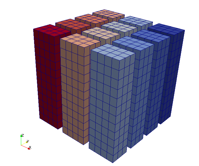
(a) Pencils in 2D decomposition aligned in $z$-direction.

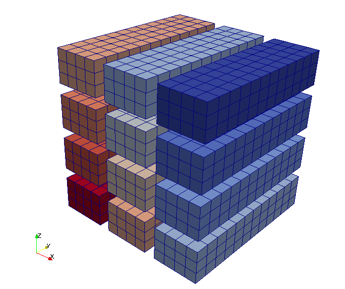
(b) Pencils in 2D decomposition aligned in $y$-direction.

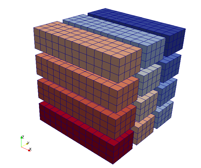
(c) Pencils in 2D decomposition aligned in $x$-direction.

Figure 4: 2D pencil decomposition on a $3\times 4$ process grid for three different alignments of a global 3D array. Each local subarray (or pencil) is colored in correspondence to the owning process, from red (process $0$) to blue (process $11$).

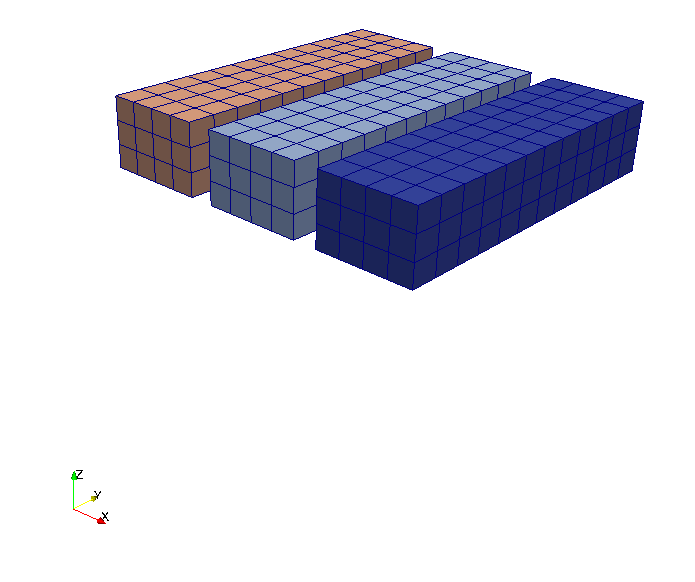
(a) Top subslab of Fig. 4(b).

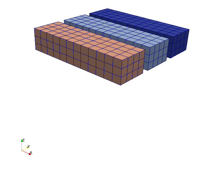
(b) Top subslab of Fig. 4(c).

Figure 5: Subslabs within a 2D pencil decomposition, corresponding to one of the subgroups $P_{0}$ with process $\{3,7,11\}$, before (a) and after (b) a global redistribution from $y$-alignment to $x$-alignment.

At first glance, the pencil method in Eqs. (21–25) looks substantially more complex to implement than the slab method in Eqs. (12–14). This is indeed the case in traditional implementations following the approach of Sec. 3.3.1. Codes typically accumulate hundreds of lines with tedious nested loops just to implement local remappings for the various possible alignments. Furthermore, these pieces of code are usually hardwired to work in the three-dimensional case, and generalizations to higher dimensions are a daunting task. At this point, with the support of Fig. 5, we make a key although simple observation: a 2D pencil decomposition can be reinterpreted as a collection of slab decompositions on one-dimensional process subgroups of the two-dimensional process grid. The consequence is remarkable: global redistribution operations like the ones in Eqs. (22) and (24) can be performed just by concurrently executing Alg. 3 on subslabs within each process subgroup. After constructing one-dimensional process subgroups as in Listing 4, the pseudocodes and listings presented in Sec. 3.3.2 can be reused verbatim to perform the two global redistribution steps required in the 2D pencil method. See Appendix A for a C code listing showcasing full forward and backward complex-to-complex transforms of a three-dimensional array with 2D pencil decomposition.

3.6 Higher-dimensional decompositions

A $d$-dimensional array can be distributed on at most $(d-1)$-dimensional process grids, such that an initial partial FFT can be performed in at least one non-distributed direction. Subsequent global redistributions and partial transforms follow to complete a full multidimensional parallel FFT. The reinterpretation of pencil decompositions as collections of slab decompositions generalizes to higher-dimensional arrays and process grids. Once again, the pseudocodes and listings presented in Secs. 3.3 and 3.4 can be reused verbatim to perform any global redistribution step.

As a proof of concept, consider a parallel FFT of a four-dimensional array, $u_{j_{0},j_{1},j_{2},j_{3}}$, using a three-dimensional process grid decomposed in the various one-dimensional process subgroups $P_{0}$, $P_{1}$ and $P_{2}$. These process subgroups can be generated with Listing 4. We perform a parallel FFT on such an array in seven steps (four partial transforms and three global redistributions) as follows:

$$\tilde{u}_{j_{0}/P_{0},j_{1}/P_{1},j_{2}/P_{2},k_{3}} =\mathcal{F}_{3}\left(u_{j_{0}/P_{0},j_{1}/P_{1},j_{2}/P_{2},j_{3}}\right),$$ (26)

$$\tilde{u}_{j_{0}/P_{0},j_{1}/P_{1},j_{2},k_{3}/P_{2}} \xleftarrow[P_{2}]{3\rightarrow 2}\tilde{u}_{j_{0}/P_{0},j_{1}/P_{1},j_{2}/P_{2},k_{3}},$$ (27)

$$\tilde{u}_{j_{0}/P_{0},j_{1}/P_{1},k_{2},k_{3}/P_{2}} =\mathcal{F}_{2}(\tilde{u}_{j_{0}/P_{0},j_{1}/P_{1},j_{2},k_{3}/P_{2}}),$$ (28)

$$\tilde{u}_{j_{0}/P_{0},j_{1},k_{2}/P_{1},k_{3}/P_{2}} \xleftarrow[P_{1}]{2\rightarrow 1}\tilde{u}_{j_{0}/P_{0},j_{1}/P_{1},k_{2},k_{3}/P_{2}},$$ (29)

$$\tilde{u}_{j_{0}/P_{0},k_{1},k_{2}/P_{1},k_{3}/P_{2}} =\mathcal{F}_{1}(\tilde{u}_{j_{0}/P_{0},j_{1},k_{2}/P_{1},k_{3}/P_{2}}),$$ (30)

$$\tilde{u}_{j_{0},k_{1}/P_{0},k_{2}/P_{1},k_{3}/P_{2}} \xleftarrow[P_{0}]{1\rightarrow 0}\tilde{u}_{j_{0}/P_{0},k_{1},k_{2}/P_{1},k_{3}/P_{2}},$$ (31)

$$\hat{u}_{k_{0},k_{1}/P_{0},k_{2}/P_{1},k_{3}/P_{2}} =\mathcal{F}_{0}(\tilde{u}_{j_{0},k_{1}/P_{0},k_{2}/P_{1},k_{3}/P_{2}}).$$ (32)

The global redistribution steps in Eqs. (27), (29) and (31) can be performed with concurrent executions of Alg. 3 on the proper subslabs corresponding to each process subgroup. See Appendix B for a C code listing showcasing full forward and backward complex-to-complex transforms of a four-dimensional array with three-dimensional decomposition.

Note that all intermediate arrays in Eqs. (26–32) must be preallocated before the 4D parallel FFT can be executed, since the global redistribution steps are out-of-place. In Appendix B four arrays are preallocated since there are four differently shaped arrays in (26–32) for a complex-to-complex transform. This may seem like excessive use of memory. However, since all intermediate arrays can be allocated in contiguous memory, the method could, in practice, simply use the two largest intermediate arrays as work buffers for all intermediate steps, regardless of dimensionality.

4 Performance evaluation

We will now explore the efficiency of the new global redistribution method proposed in previous sections. We first want to remind the reader that what is proposed is really a black-box method applicable to any array dimensionality and processor mesh decomposition. The executable code required is shown to be approximately 50 lines of code in C. Considering the complexity normally associated with this task (local transposes with or without changes of strides, in-place or out-of-place), and the thousands of lines of code dedicated to global redistribution by other parallel FFT vendors, there is at the outset of this section something to be said for simplicity.

With the current proposed method the global redistribution is achieved in one single call to MPI_ALLTOALLW. The cost of this call should be compared to the entire global redistribution operation implemented by other packages, that are typically using MPI_ALLTOALL(V) merely for communication. Now, MPI_ALLTOALL(V) works on contiguous dataarrays in both ends, both for sending and receiving ranks, and there are highly optimised versions available on several architectures. On the contrary, the subarray type used by MPI_ALLTOALLW is in general discontiguous, and there are to the authors’ knowledge no architecture-specific optimizations available. This represents a significant disadvantage of the current proposed method. However, if the additional cost of the non-optimized MPI_ALLTOALLW is not higher than the time spent on local remappings by other global redistribution methods, then it can still be competitive. Note that the collective communication routines have several different implementations by different vendors. MPICH, for example, has four different implementations of MPI_ALLTOALL that are called based on the size of the involved arrays. For MPI_ALLTOALLW, on the other hand, a non-blocking MPI_ISEND/MPI_IRECV algorithm is used regardless the array size.

Computations are performed on the Shaheen Cray XC40 supercomputer, with its primary resource capable of 7.2 Petaflops peak (5.5 sustained on the HPL benchmark [24]). The computer comes with highly optimised, preinstalled versions of the MPICH and FFTW libraries, and we use these libraries for all codes. Furthermore, all codes are compiled with Cray compilers using similar compiler options, and multithreading is disabled. The Cray XC system has 6,174 dual sockets compute nodes based on 16-core Intel Haswell processors running at 2.3GHz. Each node has 128GB of DDR4 memory running at 2.3GHz. With this multicore hardware technology there are two very different communication speeds at play - the shared intra-node and the distributed inter-node communication. Within each node there are possibly 32 cores that communicate with each other using a shared in-node memory, whereas across nodes the communication uses the Cray Aries interconnect with Dragonfly topology, which requires at most three hops between any two cores globally. The Cray XC comes with several architecture-specific optimizations for MPI_ALLTOALL(V). These optimizations may be turned off using environment variable MPICH_COLL_OPT_OFF, in which case they will use the same non-blocking MPI_ISEND/MPI_IRECV as MPI_ALLTOALLW. This has not been done here.

The global redistribution method described in previous chapters only directly affects the parallel FFT in steps (13, 22, 24). Furthermore, the sequential FFTs can be performed using any FFT vendor, and we can mainly affect the efficiency by carefully obtaining optimised installations on any given platform. However, some global/local transpose operations performed by other codes are done with the purpose of speeding up the sequential FFT, e.g., by aligning data contiguously in memory before executing. Hence, we will not only look at the global redistribution, but rather the complete transform. To this end we have implemented both slab and pencil 3D codes in C, using the global redistribution code from Sec. 3. Apart from this, the implementation is quite trivial, just a matter of creating processor groups, allocating arrays of the correct shapes and planning serial FFTs. For completeness, a 3D pencil code for complex-to-complex transforms is shown in Appendix A. We compare our code with P3DFFT, FFTW and 2DECOMP&FFT, where FFTW only has the slab method implemented, and the other two are primarily advertised as pencil decomposition codes. For the parallel FFTW results, with slab decomposition, we have used fftw_mpi_plan_dft_r2c_3d and fftw_mpi_plan_dft_c2r_3d with the transposed out option. 2DECOMP&FFT has been compiled with the C preprocessor flag -DOVERWRITE. P3DFFT has been compiled using configure options ./configure --enable-cray --enable-fftw --enable-measure FC=ftn CC=cc. We have compiled both with and without the stride1 option for the global redistribution, but, since without has been found to be generally faster, only the results of the code that disables the stride1 option are reproduced here. We use FFTW_MEASURE for all codes in planning FFTs, and the pencil decomposition is as chosen by the MPI_DIMS_CREATE function. Since P3DFFT and 2DECOMP&FFT are implemented in column-major Fortran, we here use arrays of transposed dimensions as compared to the C codes. That is, when using a global array of shape $(N_{0},N_{1},N_{2})$ in C, then an array of shape $(N_{2},N_{1},N_{0})$ is used correspondingly in Fortran. Furthermore, Fortran codes use a processor mesh that has been transposed compared to the C codes. For all codes we compute performance using two nested loops. The inner loop performs 3 consecutive, uninterrupted, forward/backward transforms, and this inner loop is repeated 50 times in an outer loop, with an MPI barrier call at the outset. The measured time after the three inner loops is reduced to the maximum value across all processors. From these values we then choose to report the fastest result from the 50 outer loops, divided by 3. For our C-code, P3DFFT and 2DECOMP&FFT we also place timers around each one of the major steps involved. This is not done for FFTW, because it would require a recompilation of the code, and we want to make use of the optimised Cray version.

The first results are computed with FFT codes that come with dedicated slab implementations, using only up to 32 processor cores, such that the two different modes of communication (intra-node vs inter-node) can be easily compared. One set of simulations employs one CPU core per node, and the other employs cores from one single node. The two settings are referred to as distributed and shared simulations, respectively. We use a quite large double precision input array of global shape $700^{3}$. Figure 6 a) shows the strong scaling achieved by our C-code, FFTW and P3DFFT (compiled with option oned enabled), for both distributed and shared operations. It is evident that all codes behave somewhat similarly, showing good strong scaling in the purely distributed mode, whereas the scaling is poor for purely shared mode. For all numbers of cores our C-code is fastest, followed by P3DFFT and FFTW. For a more detailed inspection, Figure 6 b) and c) show the individual timings for P3DFFT and our C-code for global redistributions and serial FFTs, respectively. We see that P3DFFT achieves somewhat faster serial FFTs, but that a larger difference is seen for the global redistributions in b), where our method is significantly faster over the entire range of cores. Again, scaling is seen to be good only for the purely distributed inter-node mode of operation. A deeper inspection, using Cray’s perftools, reveals that the inter-node operation allows for significantly higher clock speeds, with frequencies up to 3.5GHz, compared to the intra-node operation that clocks in around 2.5GHz for the highest number of cores. This slow-down explains the poor scaling of the serial FFTs measured in Fig. 6 c). The poor performance of the shared intra-node mode of operation is well known and has been the center of much focus, especially for supercomputers, which have been moving towards multicore designs, see, e.g., Kumar et al. [25]. Consequently, MPICH comes with some relevant compiler settings, especially for MPI_ALLTOALL (e.g., MPICH_SHARED_MEM_COLL_OPT), which enables code that tries to take advantage of the shared memory. 2DECOMP&FFT has an implementation tailored to take advantage of the shared memory, to limit the number of messages being sent (so-called leader based algorithm). However, we have not made use of such multicore aware algorithms here, and 2DECOMP&FFT has been used without the shared memory option. Furthermore, we have only used MPICH with default settings.

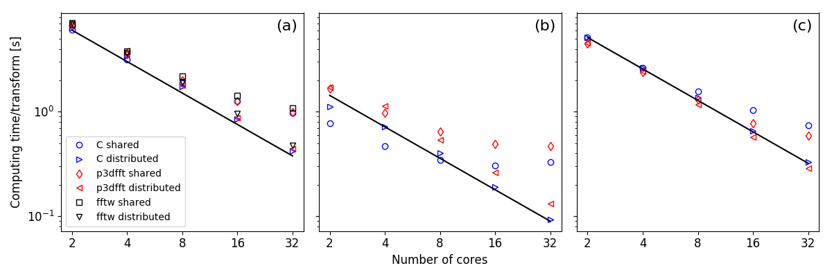
Figure 6: Strong scaling with slab decomposition of complete real-to-complex/complex-to-real FFTs on a mesh that has global shape $700^{3}$. Showing fastest times measured. The shared results correspond to shared intra-node operation, whereas distributed refer to one core per node operation. Subplot (a) shows total time, whereas (b) and (c) shows times for global redistribution and FFTs, respectively.

We next consider the pencil decomposition in purely distributed inter-node mode and perform a strong scaling study of forward and backward transforms on a global array of double precision and size $512^{3}$ in physical space. Figure 7 shows the fastest measured times for complete forward and backward transforms of our C-code, P3DFFT and 2DECOMP&FFT, for a wide scaling range. Throughout the entire range our C-code is found in a) to be 5-10 % faster than P3DFFT and 1-5 % faster than 2DECOMP&FFT. For all codes the scaling is more than excellent, achieving optimal speed per core at 256 process cores, corresponding to a mesh of size 524,288 ($64^{2}\cdot 128$) per core. Figure 7 b) and c) shows the corresponding individual timings for global redistributions and FFTs. For P3DFFT and 2DECOMP&FFT the timings for global redistributions are simply computed as the time it takes for one (forward or backward) transform minus the time spent inside sequential FFTs. It is evident from c) that the advantage of our C-code for this case is obtained through faster global redistributions, and there is little difference in computing times for sequential FFTs. The apparent superunitary scaling is explained by the higher frequencies achieved by the processors at larger core counts.

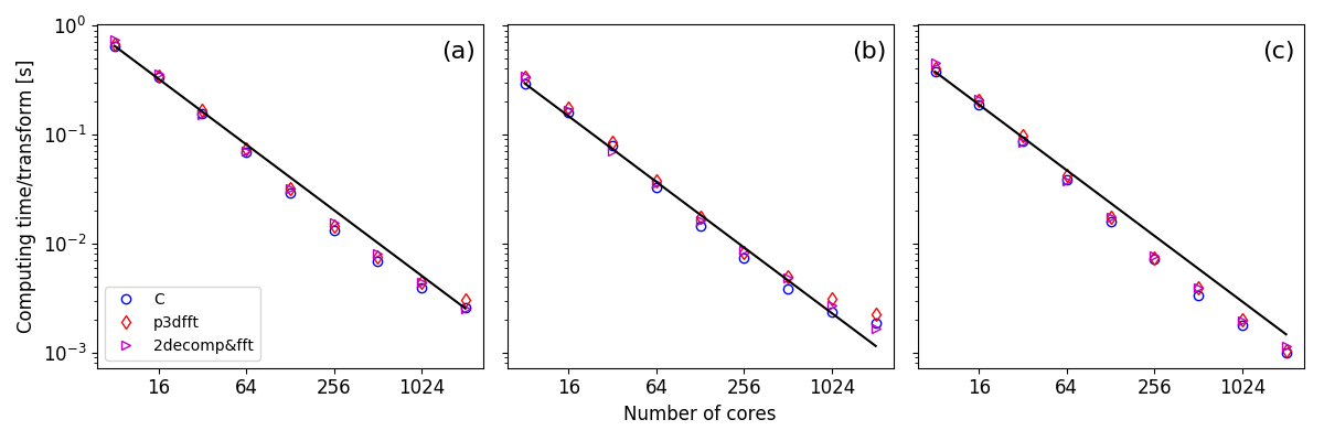
Figure 7: Strong scaling with pencil decomposition of complete real-to-complex/complex-to-real FFTs on a mesh that has global shape $512^{3}$. Showing fastest times measured. Subplot (a) shows total time, whereas (b) and (c) shows times for global redistribution and FFTs, respectively.

Next we perform a weak scaling study, using local arrays of double precision and a size (524,288) corresponding to a grid of shape $64^{2}\cdot 128$ in real space, because in the previous strong test (Fig. 7) the Shaheen computer was found to be most efficient (speed per core) for arrays of this size. We consider first the slab decomposition, and compare to the fastest results obtained with FFTW and P3DFFT in Figure 8. We observe in a) that the new C-code is equally fast as FFTW for small processor counts (4, 8, 16), and faster for higher (32 to 512). P3DFFT is fastest for the highest number of cores, where each slab is only one layer thick, but generally 5-10% slower the other runs. FFTW scales poorly at higher than 128 cores, but it is apparent that also the new method scales rather poorly in this limit of very thin slabs, i.e., when we approach the maximum number of cores possible for the slab method. P3DFFT is showing the best scaling in this limit. The major reason for the faster results obtained with the new method on low counts is found when we isolate the global redistributions. The computing times spent on global (and local) redistributions (i.e., computing time outside sequential FFTs) are shown in Figure 8 b). Again it is evident that the new method is not highly efficient in the limit of very this slabs, but all over, the global redistributions are approximately 40-50% faster than for P3DFFT. To complete the picture, we also plot the fastest computing time for the sequential FFTs in Fig. 8 c). Here it is evident that some of the sequential transforms are faster with P3DFFT, possibly because of the alignment of intermediate arrays. But the faster serial FFTs are not sufficiently much better that they can close the gap introduced by the global redistributions.

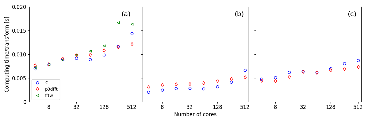
Figure 8: Weak scaling of slab decomposition of complete real-to-complex/complex-to-real FFT on a mesh that is $524,288$ per processor. Showing fastest time measured. Subplot (a) shows total time, whereas (b) and (c) shows times for global redistribution and FFTs, respectively.

We now perform the same weak efficiency test for the pencil decomposition. Figure 9 shows the fastest recorded times for a complete forward and backward transform. We see that our method is slightly faster than both P3DFFT and 2DECOMP&FFT for most measured core counts, but that differences are small. Breaking it down further, Fig. 9 c) shows the weak scaling (fastest recorded over 50 outer loops, 3 inner) for the sum of the 6 sequential FFTs required to do the forward and backward transforms. We note that there is hardly any difference at all between the codes over the entire range of the study. Figure 9 b) shows the total cost of global redistribution steps (22) and (24) for one forward and one backward transform. As for the total transform, Fig. 9 a), our C-code is fastest for low core counts, whereas there is less separating the codes for core counts larger than 128.

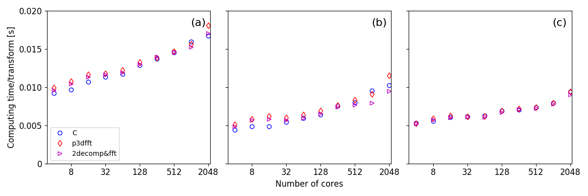
Figure 9: Weak scaling of pencil decomposition for complete real-to-complex/complex-to-real FFT on a mesh that is size $524,288$ per processor. Showing fastest times measured. Subplot (a) shows total time, whereas (b) and (c) shows times for global redistribution and FFTs, respectively.

Figures 7, 8 and 9 have been generated in the fully distributed, inter-node mode of operation. This mode is the fastest per core, but for supercomputers one normally has to pay CPU-hours for the entire node, even if only one core is used per node. For this reason it is also important to investigate the performance of the mixed multicore (inter- and intra-node) communication mode. To this end Fig. 10 shows the strong scaling of our C-code, P3DFFT and 2DECOMP&FFT for a global mesh of shape $2048^{3}$ in real space, using 16 cores per node. Here it is evident that the MPI_ALLTOALL(V) based global redistribution is faster, at least when the mesh per node is large. There is less separating the methods as the number of cores increases, where there is less work on each node.

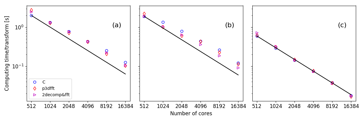
Figure 10: Strong scaling of pencil decomposition for complete real-to-complex/complex-to-real FFT on a mesh with global shape $2048^{3}$. Using 16 cores per node for mixed multicore (inter- and intra-node) communication. Showing fastest times measured. Subplot (a) shows total time, whereas (b) and (c) shows times for global redistribution and FFTs, respectively.

Finally, as a proof of concept, we consider a transform of a 4-dimensional array, that can be performed with 3 processor groups as shown in Sec 3.6. We compare in Fig. 11 the strong scaling of one forward and backward transform to the time used by PFFT on a real array of size $128^{4}$. The mesh decomposition is for both codes as chosen by MPI_DIMS_CREATE. Evidently, for this case our C-code is approximately $5-15\,\%$ faster for the number of processors ranging from 128 to 4096.

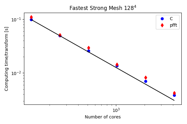
Figure 11: Strong scaling of complete real-to-complex FFT on a mesh that is size $128^{4}$, using a 3D processor mesh. Showing fastest time measured.

5 Conclusions

We presented a new and straightforward approach to implement global redistributions of arrays required in, but not limited to, parallel multidimensional fast Fourier transforms. Our approach is based on MPI subarray datatypes and generalised all-to-all scatter/gather (MPI_ALLTOALLW) collective communications, effectively eliminating any local array permutations as required in traditional implementations. Overall, our implementation amounts to less than 100 lines of simple and readable C code taking advantage of high-level MPI-2 features. Despite such conciseness, our method can perform global redistributions of $d$-dimensional arrays on up to $(d-1)$-dimensional process grids between arbitrary pairs of directions.

We performed a range of strong and weak scaling tests on Shaheen II, a Cray XC40 system at KAUST, to compare the performance of our method against other well stablished, mature alternatives like FFTW, PFFT, P3DFFT, and 2DECOMP&FFT. Despite MPI_ALLTOALLW lacking the optimizations of other all-to-all collectives, wall-clock time measurements show that our implementation is on par with the competitors.

An implementation of the approach discussed in this paper is publicly available in the open-source Python package mpi4py-fft [26]. This package is at the core of shenfun [27], a Python-based framework generalizing the spectral Galerkin method for solving partial differential equations on tensor-product spaces of arbitrary dimension. Or plans for future work are geared towards reaching wider audiences by developing a C library with Fortran wrappers and a software quality level on par with FFTW.

appendix.0appendix.0AppendixAppendixappendix.0

Appendix A Full 3D complex FFT with 2D pencil decomposition

⬇

10#include <stdlib.h>

11#include <assert.h>

12#include <complex.h>

13#include <math.h>

14#include <mpi.h>

15

16// External routine in charge of computing

17// multidimensional complex FFTs in-place

18enum { FORWARD=-1, BACKWARD=+1 };

19extern void seqxfftn(int ndims, int sizes[ndims],

20 double complex *array,

21 int axis, int sign);

22

23// Helper function to compute local sizes

24static int lsz(int N, MPI_Comm comm)

25{

26 int size, rank, n, s;

27 MPI_Comm_size(comm, &size);

28 MPI_Comm_rank(comm, &rank);

29 decompose(N, size, rank, &n, &s);

30 return n;

31}

32

33// Helper macros

34#define product(n) (n[0]*n[1]*n[2])

35#define allocate(t,n) malloc(product(n)*sizeof(t))

36#define deallocate(a) free(a)

37

38int main(int argc, char *argv[])

39{

40 MPI_Init(&argc, &argv);

41

42 // Define global 3D array sizes

43 int N[3] = {42, 127, 256};

44

45 // Create subgroups from 2D process grid

46 MPI_Comm P[2];

47 subcomm(MPI_COMM_WORLD, 2, P);

48

49 // Define elementary MPI datatype

50 MPI_Datatype T = MPI_C_DOUBLE_COMPLEX;

51

52 // Define local sizes and allocate local 3D arrays

53 int sizesA[3] = {lsz(N[0],P[0]), lsz(N[1],P[1]), N[2]};

54 int sizesB[3] = {lsz(N[0],P[0]), N[1], lsz(N[2],P[1])};

55 int sizesC[3] = {N[0], lsz(N[1],P[0]), lsz(N[2],P[1])};

56 double complex *arrayA = allocate(double complex, sizesA);

57 double complex *arrayB = allocate(double complex, sizesB);

58 double complex *arrayC = allocate(double complex, sizesC);

59

60 for (int j=0, n=product(sizesA); j<n; j++)

61 arrayA[j] = j + j * I; // Fill array with complex values

62

63 // Forward FFT

64 seqxfftn(3, sizesA, arrayA, 2, FORWARD);

65 exchange(P[1], T, 3, sizesA, arrayA, 2, sizesB, arrayB, 1);

66 seqxfftn(3, sizesB, arrayB, 1, FORWARD);

67 exchange(P[0], T, 3, sizesB, arrayB, 1, sizesC, arrayC, 0);

68 seqxfftn(3, sizesC, arrayC, 0, FORWARD);

69

70 // Backward FFT

71 seqxfftn(3, sizesC, arrayC, 0, BACKWARD);

72 exchange(P[0], T, 3, sizesC, arrayC, 0, sizesB, arrayB, 1);

73 seqxfftn(3, sizesB, arrayB, 1, BACKWARD);

74 exchange(P[1], T, 3, sizesB, arrayB, 1, sizesA, arrayA, 2);

75 seqxfftn(3, sizesA, arrayA, 2, BACKWARD);

76

77 for (int j=0, n=product(sizesA); j<n; j++) // Check result

78 assert(fabs(creal(arrayA[j]) - j) < 1.0e-8 &&

79 fabs(cimag(arrayA[j]) - j) < 1.0e-8);

80

81 deallocate(arrayA);

82 deallocate(arrayB);

83 deallocate(arrayC);

84 MPI_Comm_free(&P[0]);

85 MPI_Comm_free(&P[1]);

86

87 MPI_Finalize();

88 return 0;

89}

Appendix B Full 4D complex FFT with 3D decomposition

⬇

#include <stdlib.h>

#include <assert.h>

#include <complex.h>

#include <math.h>

#include <mpi.h>

// External routine in charge of computing

// multidimensional complex FFTs in-place

enum { FORWARD=-1, BACKWARD=+1 };

extern void seqxfftn(int ndims, int sizes[ndims],

double complex *array,

int axis, int sign);

// Helper function to compute local sizes

static int lsz(int N, MPI_Comm comm)

{

int size, rank, n, s;

MPI_Comm_size(comm, &size);

MPI_Comm_rank(comm, &rank);

decompose(N, size, rank, &n, &s);

return n;

}

// Helper macros

#define product(n) (n[0]*n[1]*n[2]*n[3])

#define allocate(t,n) malloc(product(n)*sizeof(t))

#define deallocate(a) free(a)

int main(int argc, char *argv[])

{

MPI_Init(&argc, &argv);

// Define global 4D array sizes

int N[4] = {16, 17, 18, 19};

// Create subgroups from 3D process grid

MPI_Comm P[3];

subcomm(MPI_COMM_WORLD, 3, P);

// Define elementary MPI datatype

MPI_Datatype T = MPI_C_DOUBLE_COMPLEX;

// Define local sizes

int sizesA[4] = {lsz(N[0],P[0]), lsz(N[1],P[1]),

lsz(N[2],P[2]), N[3]};

int sizesB[4] = {lsz(N[0],P[0]), lsz(N[1],P[1]),

N[2], lsz(N[3],P[2])};

int sizesC[4] = {lsz(N[0],P[0]), N[1],

lsz(N[2],P[1]), lsz(N[3],P[2])};

int sizesD[4] = {N[0], lsz(N[1],P[0]),

lsz(N[2],P[1]), lsz(N[3],P[2])};

// Allocate local 3D arrays

double complex *arrayA = allocate(double complex, sizesA);

double complex *arrayB = allocate(double complex, sizesB);

double complex *arrayC = allocate(double complex, sizesC);

double complex *arrayD = allocate(double complex, sizesD);

for (int j=0, n=product(sizesA); j<n; j++)

arrayA[j] = j + j * I; // Fill array with complex values

// Forward FFT

seqxfftn(4, sizesA, arrayA, 3, FORWARD);

exchange(P[2], T, 3, sizesA, arrayA, 3, sizesB, arrayB, 2);

seqxfftn(4, sizesB, arrayB, 2, FORWARD);

exchange(P[1], T, 3, sizesB, arrayB, 2, sizesC, arrayC, 1);

seqxfftn(4, sizesC, arrayC, 1, FORWARD);

exchange(P[0], T, 3, sizesC, arrayC, 1, sizesD, arrayD, 0);

seqxfftn(4, sizesD, arrayD, 0, FORWARD);

// Backward FFT

seqxfftn(4, sizesD, arrayD, 0, BACKWARD);

exchange(P[0], T, 3, sizesD, arrayD, 0, sizesC, arrayC, 1);

seqxfftn(4, sizesC, arrayC, 1, BACKWARD);

exchange(P[1], T, 3, sizesC, arrayC, 1, sizesB, arrayB, 2);

seqxfftn(4, sizesB, arrayB, 2, BACKWARD);

exchange(P[2], T, 3, sizesB, arrayB, 2, sizesA, arrayA, 3);

seqxfftn(4, sizesA, arrayA, 3, BACKWARD);

for (int j=0, n=product(sizesA); j<n; j++) // Check result

assert(fabs(creal(arrayA[j]) - j) < 1.0e-8 &&

fabs(cimag(arrayA[j]) - j) < 1.0e-8);

deallocate(arrayA);

deallocate(arrayB);

deallocate(arrayC);

deallocate(arrayD);

MPI_Comm_free(&P[0]);

MPI_Comm_free(&P[1]);

MPI_Comm_free(&P[2]);

MPI_Finalize();

return 0;

}

References

- [1] I. T. Foster, P. H. Worley, Parallel algorithms for the spectral transform method, SIAM Journal on Scientific Computing 18 (3) (1997) 806–837. doi:10.1137/S1064827594266891.
- [2] A. Gupta, V. Kumar, The scalability of FFT on parallel computers 4 (8) (1993) 922–932. doi:10.1109/71.238626.
- [3] H. Q. Ding, R. D. Ferraro, D. B. Gennery, A portable 3D FFT package for distributed-memory parallel architectures, in: Proceedings of 7th SIAM Conference on Parallel Processing, SIAM Press, 1995, pp. 70–71.
- [4] D. Pekurovsky, P3DFFT: a framework for parallel computations of Fourier transforms in three dimensions, SIAM Journal on Scientific Computing 34 (4) (2012) 192–209. doi:10.1137/11082748X.
- [5] N. Li, S. Laizet, 2DECOMP&FFT - a highly scalable 2d decomposition library and FFT interface, in: CUG 2010 Proceedings, Cray User Group, 2010.
- [6] M. Pippig, PFFT: An extension of FFTW to massively parallel architectures, SIAM Journal on Scientific Computing 35 (3) (2013) C213–C236. doi:10.1137/120885887.
- [7] M. Frigo, S. G. Johnson, The design and implementation of FFTW3, Proceedings of the IEEE 93 (2) (2005) 216–231. doi:10.1109/JPROC.2004.840301.
- [8] T. V. T. Duy, T. Ozaki, A decomposition method with minimum communication amount for parallelization of multi-dimensional FFTs, Computer Physics Communications 185 (1) (2014) 153–164. doi:10.1016/j.cpc.2013.08.028.
-
[9]
A. Gholami, J. Hill, D. Malhotra, G. Biros, AccFFT -
a new parallel FFT library.
URL http://accfft.org -
[10]
S. Plimpton,
Parallel
FFT package.
URL {http://www.sandia.gov/%7Esjplimp/docs/fft/README.html} -
[11]
J. C. Bowman, M. Roberts, FFTW++: Fast
Fourier transform C++ header/MPI transpose for FFTW3.
URL http://fftwpp.sourceforge.net -
[12]
M. Mortensen, Parallel FFT in
3D or 2D using MPI for Python.
URL https://github.com/spectralDNS/mpiFFT4py -
[13]
L. Dalcin, MPI for Python.
URL https://bitbucket.org/mpi4py/mpi4py/ - [14] L. Dalcin, R. Paz, M. Storti, J. D’Elia, MPI for Python: Performance improvements and MPI-2 extensions, Journal of Parallel and Distributed Computing 68 (5) (2008) 655–662. doi:10.1016/j.jpdc.2007.09.005.
-
[15]
Message Passing Interface Forum,
MPI: A
Message-Passing Interface Standard, Version 3.1, High Performance Computing
Center Stuttgart (HLRS), 2015.
URL http://mpi-forum.org/docs/mpi-3.1/mpi31-report.pdf - [16] T. Heofler, S. Gottlieb, Recent Advances in the Message Passing Interface, Springer, 2010, Ch. Parallel Zero-Copy Algorithms for Fast Fourier Transform and Conjugate Gradient using MPI Datatypes, pp. 132–141. doi:10.1007/978-3-642-15646-5.
-
[17]
D. Grote, J.-L. Vay, A. Friedman, S. Lund,
Warp.
URL https://sites.google.com/a/lbl.gov/warp/home -
[18]
P. N. Swarztrauber, FFTPACK.
URL http://www.netlib.org/fftpack/ -
[19]
IBM, Engineering and
scientific subroutine library (essl) and parallel essl.
URL http://www.ibm.com/systems/power/software/essl/ -
[20]
Intel, Math Kernel Library (MKL).
URL https://software.intel.com/mkl -
[21]
S. Balay, S. Abhyankar, M. F. Adams, J. Brown, P. Brune, K. Buschelman,
L. Dalcin, V. Eijkhout, W. D. Gropp, D. Kaushik, M. G. Knepley, D. A. May,
L. C. McInnes, R. T. Mills, T. Munson, K. Rupp, P. Sanan, B. F. Smith,
S. Zampini, H. Zhang, H. Zhang,
PETSc
users manual, Tech. Rep. ANL-95/11 - Revision 3.9, Argonne National
Laboratory (2018).
URL http://www.mcs.anl.gov/petsc/petsc-current/docs/manual.pdf - [22] M. Mortensen, H. P. Langtangen, High performance Python for direct numerical simulations of turbulent flows, Computer Physics Communications 203 (2016) 53–65. doi:10.1016/j.cpc.2016.02.005.
- [23] W. Gropp, T. Hoefler, R. Thakur, E. Lusk, Using Advanced MPI: Modern Features of the Message-Passing Interface, The MIT Press, 2014.
-
[24]
Shaheen II CrayXC40 - Top 500 list
- November 2017.
URL https://www.top500.org/system/178515 - [25] R. Kumar, A. Mamidala, D. K. Panda, Scaling alltoall collective on multi-core systems, in: 2008 IEEE International Symposium on Parallel and Distributed Processing, IEEE, 2008, pp. 1–8. doi:10.1109/IPDPS.2008.4536141.
-
[26]
L. Dalcin, M. Mortensen,
mpi4py-fft.
URL https://bitbucket.org/mpi4py/mpi4py-fft - [27] M. Mortensen, Shenfun – automating the spectral Galerkin method, ArXiv e-printsarXiv:1708.03188.
appendix.0appendix.0\EdefEscapeHexAppendixAppendix\hyper@anchorstartappendix.0\hyper@anchorend