Scale independence in an asymptotically free theory at finite temperatures

Abstract

A recently developed variational resummation technique incorporating renormalization group properties has been shown to solve the scale dependence problem that plagues the evaluation of thermodynamical quantities, e.g., within the framework of approximations such as in the hard-thermal-loop resummed perturbation theory. This method is used in the present work to evaluate thermodynamical quantities within the two-dimensional nonlinear sigma model, which shares some features with Yang-Mills theories like asymptotic freedom, trace anomaly and the nonperturbative generation of a mass gap. Besides the fact that nonperturbative results can be readily generated solely by considering the lowest-order contribution to the thermodynamic effective potential, we also show that its next-to-leading correction indicates convergence to the sought-after scale invariance.

I Introduction

The theoretical description of the quark-gluon plasma phase transition requires the use of nonperturbative methods, since the use of perturbation theory near the transition is unreliable. LQCD has been very successful at finite temperatures and near vanishing baryonic densities, however, currently, the complete description of compressed baryonic matter cannot be achieved due to the so-called sign problem. In this case, an alternative is to use approximate but more analytical nonperturbative approaches. One of these is the Optimized Perturbation Theory (OPT), which reorganizes the series using a variational approximation, where the result of a related solvable case is rewritten in terms of a variational parameter that allows for nonperturbative results to be obtained. On the other hand, the results of the Hard Thermal Loop Perturbation Theory (HTLpt), done in a gauge-invariant framework, exhibit a strong sensitivity to the arbitrary renormalization scale M used in the regularization procedure HTLPT3loop . A solution to this problem has been recently proposed, by generalizing to thermal theories a related variational resummation approach, Renormalization Group Optimized Perturbation Theory (RGOPT) JLGN . In this work we apply the RGOPT to the nonlinear sigma model (NLSM) in 1+1 dimensions at finite temperatures in order to pave the way for future applications concerning other asymptotically free theories, such as thermal QCD. As we will illustrate, the scale invariant results obtained in the present application give further support to the method as a robust analytical nonperturbative approach to thermal theories.

II The NLSM in 1+1-dimensions

The two-dimensional NLSM partition function can be written as nlsmrenorm

$$Z\!=\!\int\!\prod_{i=1}^{N}{\cal D}\Phi_{i}(x)\exp\left[\frac{1}{2g_{0}}\!\!\int\!d^{2}x(\partial\Phi_{i})^{2}\right]\delta(\sum_{i=1}^{N}\Phi_{i}\Phi_{i}-1),$$ (1)

where $g_{0}$ is a (dimensionless) coupling and the scalar field is parametrized as $\Phi_{i}=(\sigma,\pi_{1},...,\pi_{N-1})$. In two-dimensions the theory is renormalizable nlsmrenorm . The action is invariant under $O(N)$ but using the constraint, $\sigma(x)=(1-\pi_{i}^{2})^{1/2}$, in order to define the perturbative expansion, breaks the symmetry down to $O(N-1)$. In this case the partition function becomes

$$Z(m)=\int d\pi_{i}(x)\left[1-\pi_{i}^{2}(x)\right]^{-1/2}\exp[-{\cal S}(\pi,m)],$$ (2)

where the (Euclidean) action is ${\cal S}(\pi,m)=\int d^{2}x{\cal L}_{0}$ and, upon rescaling $\pi_{i}\to\sqrt{g_{0}}\pi_{i}$, we can read the bare Lagrangian density and expand it to order-$g_{0}$ yielding

$${\cal L}_{0}\!=\!\frac{1}{2}\left[(\partial\pi_{i})^{2}+m_{0}^{2}\pi_{i}^{2}\right]+\frac{g_{0}m_{0}^{2}}{8}(\pi_{i}^{2})^{2}+\frac{g_{0}}{2}(\pi_{i}\partial\pi_{i})^{2}-{\cal E}_{0},$$ (3)

where for later notational convenience we designate as ${\cal E}_{0}\equiv m^{2}_{0}/g_{0}$ the field-independent term, originating at lowest order from expanding the square root in the bare lagrangian.

In this work, the divergent integrals are regularized using dimensional regularization (within the minimal subtraction scheme $\overline{\rm MS}$), which at finite temperature and $d=2-\epsilon$ dimensions, can be implemented by using

$$\int\frac{d^{2}p}{(2\pi)^{2}}\to T\,\hbox{$\sum$}\!\!\!\!\!\!\!\int_{\bf p}\equiv T\left(\frac{e^{\gamma_{E}}M^{2}}{4\pi}\right)^{\epsilon/2}\sum_{n=-\infty}^{+\infty}\int\frac{d^{1-\epsilon}p}{(2\pi)^{1-\epsilon}},$$ (4)

where $\gamma_{E}$ is the Euler-Mascheroni constant and $M$ is the $\overline{\rm MS}$ arbitrary regularization energy scale.

III Perturbative Pressure and Scale Invariance

Figure 1: Feynman diagrams contributing to the perturbative pressure at ${\cal O}(g)$. The first term represents $P_{0}(m_{0})$, the second, $P_{1}(m_{0},g_{0})$, the third term represents the self-energy counterterm $P_{0}^{\rm CT}$ (obtained from expanding $Z_{m}$ to first order in $P_{0}(m_{0}=Z_{m}\,m)$), while the fourth term represents the zero point contribution ${\cal E}_{0}(g_{0})$ to Eq. (5).

Considering the contributions displayed in Fig. 1, one can write the pressure up to order ${\cal O}(g_{0})$ as

$$P=P_{0}(m_{0})+P_{1}(m_{0},g_{0})+{\cal E}_{0}(m_{0},g_{0})+{\cal O}(g_{0}^{2}).$$ (5)

By implementing renormalization consistently after the identification of the counterterms (details can be found on ournlsm ), the renormalized two-loop pressure can be written in its compact form

$$P=\frac{m^{2}}{g}-\frac{(N-1)}{2}\left[I_{0}^{\rm r}(m,T)+\frac{(N-3)}{4}m^{2}g\left[I_{1}^{\rm r}(m,T)\right]^{2}\right],$$ (6)

where

$$I_{0}(m_{0},T)=T\,\hbox{$\sum$}\!\!\!\!\!\!\!\int_{\bf p}\ln\left(\omega_{n}^{2}+\omega_{\bf p}^{2}\right),$$ (7)

with the dispersion relation, $\omega_{\bf p}^{2}={\bf p}^{2}+m_{0}^{2}$ and $I_{1}(m_{0},T)=\partial I_{0}(m_{0},T)/\partial m_{0}^{2}$.

Considering the renormalization group (RG) operator, defined by

$$M\frac{d}{dM}\equiv M\frac{\partial}{\partial M}+\beta\frac{\partial}{\partial g}-\frac{n}{2}\zeta+\gamma_{m}m\frac{\partial}{\partial m}.$$ (8)

Applying the latter to the pressure (zero-point vacuum energy) one has $n=0$, so that one only needs to consider the $\beta$ and $\gamma_{m}$ functions. At the two-loop level,

$$\beta=-b_{0}g^{2}-b_{1}g^{3}+{\cal O}(g^{4}),$$ (9)

and

$$\gamma_{m}=-\gamma_{0}g-\gamma_{1}g^{2}+{\cal O}(g^{3}),$$ (10)

where the RG coefficients in our normalization are hikami :

$$b_{0}=(N-2)/(2\pi),$$ (11)

$$b_{1}=(N-2)/(2\pi)^{2},$$ (12)

$$\gamma_{0}=(N-3)/(8\pi),$$ (13)

$$\gamma_{1}=(N-2)/(8\pi^{2}).$$ (14)

Following jlprl one can write the finite zero-point energy contribution, ${\cal E}_{0}^{\rm RG}$:

$${\cal E}_{0}^{\rm RG}=m^{2}\sum_{k\geq 0}s_{k}g^{k-1},$$ (15)

and determine the coefficients $s_{k}$ by applying (8) consistently order by order. In the present NLSM, one can easily check that it uniquely fixes the relevant coefficients up to two-loop order, $s_{0},s_{1}$, as

$$s_{0}=\frac{(N-1)}{4\pi(b_{0}-2\gamma_{0})}=1,$$ (16)

and

$$s_{1}=(b_{1}-2\gamma_{1})\frac{s_{0}}{2\gamma_{0}}=0,$$ (17)

(which vanishes as $b_{1}=2\gamma_{1}$ in the NLSM).
Thus from perturbative RG considerations, Eq. (15) with (16), (17) reconstructs consistently the NLSM first term of (6), originally present in our original NLSM derivation above. RG invariance is maintained (or more correctly, restored) also within the more drastic modifications implied by the variationally optimized perturbation framework, as we examine now.

IV RG Improved Optimized Perturbation Theory

To implement next the RGOPT one first modify the standard perturbative expansion by rescaling the infrared regulator $m$ and coupling:

$$m\to(1-\delta)^{a}m,\;\;\;\;g\to\delta g,$$ (18)

in such a way that the Lagrangian interpolates between a free massive theory (for $\delta=0$) and the original massless theory (for $\delta=1$) JLQCD1 . Since the mass parameter is being optimized by using the variational stationary mass optimization prescription pms , as in OPT or in the Screened Perturbation Theory (SPT,  spt ),

$$\frac{\partial P^{\rm RGOPT}}{\partial m}\Bigr{|}_{m={\bar{m}}}=0,$$ (19)

the RG operator acquires the reduced form

$$\left(M\frac{\partial}{\partial M}+\beta\frac{\partial}{\partial g}\right)P^{\rm RGOPT}=0.$$ (20)

which is indeed consistent for a massless theory.

Then, performing the aforementioned replacements given by Eq. (18) within the pressure Eq. (6), consistently re-expanding to lowest (zeroth) order in $\delta$, and finally taking $\delta\to 1$, one gets

$$P^{\rm RGOPT}_{1L}=-\frac{(N-1)}{2}I_{0}^{\rm r}(m,T)+\frac{m^{2}}{g}(1-2a).$$ (21)

Now to fix the exponent $a$ we require the RGOPT pressure, Eq. (21), to satisfy the reduced RG relation, Eq. (20). This uniquely fixes the exponent to

$$a=\frac{\gamma_{0}}{b_{0}}=\frac{(N-3)}{4(N-2)}.$$ (22)

With the exponent $a$ determined, one can write the resulting one-loop RGOPT expression for the NLSM pressure as

$$P^{\rm RGOPT}_{1L}=-\frac{(N-1)}{2}I_{0}^{\rm r}(m,T)+(N-1)\frac{m^{2}}{(4\pi)gb_{0}}.$$ (23)

In the same way, the two-loop standard PT result obtained in the previous section gets modified accordingly to yield the corresponding RGOPT pressure at the next order of those approximation sequences. After performing the substitutions given by Eq. (18), with $a=\gamma_{0}/b_{0}$ within the two-loop PT pressure Eq. (6), expanding now to first order in $\delta$, next taking the limit $\delta\to 1$, gives

$$P^{\rm RGOPT}_{2L} = -\frac{(N-1)}{2}I_{0}^{\rm r}(m,T)+(N-1)\left(\frac{\gamma_{0}}{b_{0}}\right)m^{2}I_{1}^{\rm r}(m,T)$$ (24)

$$- g(N-1)\frac{(N-3)}{8}m^{2}\left[I_{1}^{\rm r}(m,T)\right]^{2}$$

$$+ \frac{(N-1)}{4\pi}\frac{m^{2}}{g\,b_{0}}\left(1-\frac{\gamma_{0}}{b_{0}}\right).$$

RGOPT mass gap and running coupling constant

By optimizing the pressures above and solving the mass gap ournlsm , at one-loop one obtains

$${\bar{m}}(0)=M\exp\left(-\frac{1}{b_{0}\,g(M)}\right).$$ (25)

It is instructive to remark that the above optimized mass gap is dynamically generated by the (nonlinear) interactions and reflects dimensional transmutation, with nonperturbative coupling dependence.

The Eq. (25) moreover fixes the optimized mass $\bar{m}$ to be fully consistent with the running coupling $g(M)$ as described by the usual one-loop result,

$$g^{-1}(M)=g^{-1}(M_{0})+b_{0}\ln\frac{M}{M_{0}},$$ (26)

where $M_{0}$ is an arbitrary reference scale and $L=\ln(M/M_{0})$.

Going now to two-loop order, the mass optimization criterion Eq. (19) applied to the RGOPT-modified two-loop pressure Eq. (24) can be cast, after straightforward algebra, in the form (omitting some irrelevant overall factors):

$$f_{MOP}^{(2L)}\equiv\left\{3N-5-b_{0}(N-3)\,g\,\left[1+Y+2x^{2}J_{2}(x)\right]\right\}$$

$$\times m\,\left(\frac{1}{b_{0}\,g}+Y\right)=0,$$ (27)

where, we have defined for convenience the following dimensionless quantity

$$Y\equiv\ln\frac{m}{M}+2J_{1}(x)=-2\pi\,I_{1}^{r}(m,T),$$ (28)

and the thermal integral, $xJ_{2}(x)\equiv\partial_{x}J_{1}(x)$ reads

$$J_{2}(x)=\int_{0}^{\infty}dz\frac{[e^{\omega_{z}}(1+\omega_{z})-1]}{\omega_{z}^{3}(1-e^{\omega_{z}})^{2}}.$$ (29)

Alternatively, the reduced RG equation (20), using the exact two-loop $\beta$-function Eq. (9), yields

$$f_{RG}^{(2L)}\equiv m^{2}\,\left[g\frac{(3N-5)}{2\pi}+(N-3)\times\right.$$

$$\left.\left\{1+\frac{N-2}{\pi}g\,Y\left[1+\frac{N-2}{4\pi}g\,(1+\frac{g}{2\pi})\,Y\right]\right\}\right]=0.$$ (30)

When considered as two alternative (separate) equations, (27) and (30), apart from having the trivial solution $\bar{m}=0$, also have a more interesting nonzero mass gap solution, $\bar{m}(g,T,M)$, with nonperturbative dependence on the coupling $g$.

Hence, apart from the one-loop running in Eq. (26), we also need the two-loop running coupling, with exact expression given e.g. in  jlprd , which can be approximated as follows with sufficient accuracy (as long as $g$ remains rather moderate $g\sim{\cal O}(1)$),

$$g^{-1}(M) \simeq g^{-1}(M_{0})+b_{0}L+(b_{1}L)g(M_{0})$$ (31)

$$- \left(\frac{1}{2}b_{0}b_{1}L^{2}\right)g^{2}(M_{0})$$

$$- \left(\frac{1}{2}b_{1}^{2}L^{2}-\frac{1}{3}b_{0}^{2}b_{1}L^{3}\right)g^{3}(M_{0})$$

$$+ {\cal O}(g^{4}).$$

V Numerical Results

To investigate and compare the scale variation behavior of the different approximations - such as large-$N$ (LN) and SPT - in our analysis below, as it is customary, we set the arbitrary $\overline{\rm MS}$ scale as $M=\alpha M_{0}=2\pi T\alpha$ and consider $0.5\leq\alpha\leq 2$ as representative values of scale variations. On ournlsm one can find the explanation of the residual scale dependence and a complete description of the parameters choice regarding the coupling.

The RGOPT mass ${\bar{m}}(T)$ clearly starts from a nonzero value at $T=0$, since the mass gap solution is nontrivial at $T=0$ (Eq. (25)), then bends and reaches, as expected by using basic dimensional arguments, a straight line for large temperatures, where it behaves perturbatively as $\bar{m}\sim gT$. As observed in giacosa , this behavior is reminiscent of that of the gluon mass in the deconfined phase of Yang-Mills theories YM1 , where, at high-$T$, the gluon mass can be parametrized by $T/\ln T$. The bending of the thermal masses can be better appreciated in Fig. 2, which shows that the changing of behavior occurs at rather low temperatures.

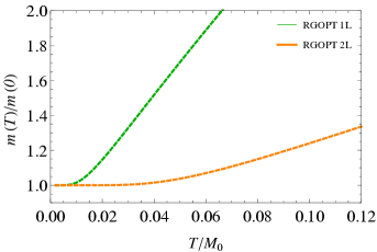
Figure 2: The normalized thermal optimized masses, ${\bar{m}}(T)/{\bar{m}}(0)$, as a function of the temperature $T$ (normalized by $M_{0}$) for $N=4$, $g(M_{0})=1=g_{LN}(M_{0})/2$, and at the central scale choice $\alpha=1$, in the RGOPT at one- and two-loop cases. (NB for this coupling choice the LN thermal mass is identical to the RGOPT one-loop one).

In Fig. 3 we show the (subtracted) pressure, $P=P(T)-P(0)$, normalized by $P_{\rm SB}$, for the scale variations $M=\alpha M_{0}$, $0.5\leq\alpha\leq 2$ and $N=4$. It illustrates how the one-loop RGOPT pressure is exactly scale invariant, while the two-loop result displays a (small) residual scale dependence for the construction of the method (see ournlsm for details). The RGOPT pressure itself exhibits a substantially smaller scale dependence than the corresponding SPT approximation, at moderate and low $T/M_{0}$ values, as can be seen on Fig. (3). On ournlsm we propose a temperature-dependent coupling $g(T)$ to minimize this moderate residual scale dependence within the two-loop results.

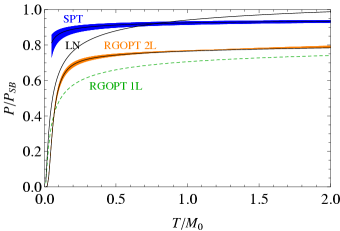
Figure 3: $P/P_{\rm SB}$ as function of the temperature $T$ (normalized by $M_{0}$) for $N=4$ and $g(M_{0})=1=g_{LN}(M_{0})/2$, with scale variation $0.5\leq\alpha\leq 2$. Within the two-loop RGOPT and SPT, the shaded bands have the lower edge for $\alpha=0.5$ and the upper edge for $\alpha=2$. The thin line inside the shaded bands is for $\alpha=1$.

We will now compare the RGOPT results with lattice simulation ones. To the best of our knowledge, recently the only available lattice thermodynamics simulation of the NLSM is the one of giacosa , which was performed for $N=3$. To complete this comparison, we need a priori to fix an appropriate coupling value at some scale $M_{0}$, recalling that the simulation in giacosa was performed at relatively strong lattice coupling values. In the RGOPT framework, similarly to the LN approximation, as we have explained the constant vacuum energy piece $m^{2}/g$ (footprint of a $\sigma$ field term), plays a crucial role in obtaining a mass gap with these expected features of the low-$T$ nonperturbative NLSM properties. While at asymptotically high-$T$ one reaches the free theory $g\to 0$ limit of the NLSM model, thus describing a gas of $N-1$ non-interacting pions, while the non-kinetic $m^{2}/g$ contribution becomes negligible. The RGOPT two-loop results roughly exhibit this overall nonperturbative behavior from low- to high-$T$ regime (although not perfectly at very low temperatures). In Fig. 4 we thus compare the one- and two-loop RGOPT and the LN pressure for $g(M_{0})=2\pi$ with the lattice data for $N=3$, as function of the temperature, now normalized by the $T=0$ mass gap $\bar{m}(0)$, consistently with the lattice results normalizationgiacosa . A clear explanation concerning some peculiarities about the $N$ choice can be found on ournlsm .

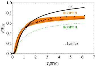
Figure 4: $P/P_{\rm SB}$ as a function of the temperature $T$ (normalized by the $T=0$ mass gap $\bar{m}(0)$) for $N=3$: LN, one- and two-loop RGOPT for $g(M_{0})=g_{LN}(M_{0})=2\pi$ and scale variation $1/2\leq\alpha\leq 2$, when using RG optimized running, compared with lattice simulations (taken from giacosa ). NB lattice data have been conveniently rescaled on vertical axis from $P/T^{2}$ in giacosa to $P/P_{SB}$ (i.e., for $N=3$ this corresponds to a scaling factor of $\pi/3$).

It is also of interest to investigate the behavior of some other thermodynamical quantities evaluated in the RGOPT scheme and how they compare with the same quantities evaluated in the SPT and LN approximations. For example, the interaction measure $\Delta=({\cal E}-P)/T^{2}\equiv T\partial_{T}[P(T)/T^{2}]$, which is the trace of the energy-momentum tensor normalized by $T^{2}$. The interaction measure can be readily obtained from the pressure by using the definitions for the entropy density,

$$S=\frac{d}{d\,T}P(\bar{m}(g,T,M),T,M),$$ (32)

and for the energy density, ${\cal E}=-P+S\,T$.

In Fig. 5 we show the dependence of the interaction measure as a function of the temperature in the one- and two-loop RGOPT, two-loop SPT, and LN cases, for the same choice of $N=4$ and $g=1=g_{LN}/2$, as in the previous plots.

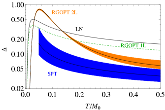
Figure 5: The interaction measure $\Delta$ as a function of the temperature $T$ (normalized by $M_{0}$) for $N=4$ and $g(M_{0})=1=g_{LN}(M_{0})/2$, with scale variation $0.5\leq\alpha\leq 2$, using the standard two-loop running coupling given by Eq. 31). Within the two-loop RGOPT and SPT, the shaded bands have the lower edge for $\alpha=0.5$ and the upper edge for $\alpha=2$. The thin line inside the shaded bands is for $\alpha=1$. (Logarithmic scale is used).

We notice from the RGOPT results shown in Fig. 5 how the inflection before the peak of $\Delta$ occurs approximately at the temperature value where $m(T)$ bends (see Fig. 2), which is an interesting feature if one recalls that in QCD the inflection occurs at $T_{c}$.

VI Conclusions

We have applied the recently developed RGOPT nonperturbative framework to investigate thermodynamical properties of the asymptotically free $O(N)$ NLSM in two dimensions, and illustrate results for $N=3$ and $N=4$. Our application shows how simple perturbative results can acquire a robust nonperturbative predictive power by combining renormalization group properties with a variational criterion used to fix the (arbitrary) “quasi-particle” RGOPT mass.

Our application shows how simple perturbative results can acquire a robust nonperturbative predictive power by combining renormalization group properties with a variational criterion used to fix the (arbitrary) “quasi-particle” RGOPT mass. A non-trivial scale invariant result was obtained by considering the lowest order contribution to the pressure and the NLO (two-loop) order RGOPT results display a very mild residual scale dependence when compared to the standard SPT/OPT results. We also obtain a reasonable agreement of the RGOPT pressure with known lattice results for $N=3$. The NLSM thermodynamical observables obtained from two-loop RGOPT display a physical behavior that is more in line with LQCD predictions for pure Yang-Mills four-dimensional theories, as compared with the two-loop order SPT. The one- and two-loop RGOPT interaction measure $\Delta$ exhibit some characteristic nonperturbative features somewhat similar to the QCD interaction measure. Finally it would be of much interest to compare our NLSM thermodynamical results with other lattice simulation results for other $N$ values, but unfortunately to our knowledge no such simulations at finite temperature are available up to now for $N>3$.

References

- (1) J. O. Andersen, L. E. Leganger, M. Strickland and N. Su, JHEP 1108, 053 (2011).
- (2) J.-L. Kneur and A. Neveu, Phys. Rev. D 81, 125012 (2010).
- (3) E. Brezin, J. Zinn-Justin and J. C. Le Guillou, Phys. Rev. D 14, 2615 (1976).
- (4) G. N. Ferrari, J.-L. Kneur, M. B. Pinto and R. O. Ramos, Phys. Rev. D 96, 116009 (2017).
- (5) S. Hikami and E. Brezin, J. Phys. A 11, 1141 (1978).
- (6) J.-L. Kneur and M. B. Pinto, Phys. Rev. Lett. 116, 031601 (2016).
- (7) J.-L. Kneur and A. Neveu, Phys. Rev. D 85, 014005 (2012).
- (8) P. M. Stevenson, Phys. Rev. D 23, 2916 (1981).
- (9) J. O. Andersen, E. Braaten and M. Strickland, Phys. Rev. D 63, 105008 (2001).
- (10) J.-L. Kneur and M. B. Pinto, Phys. Rev. D 92, 116008 (2015).
- (11) E. Seel, D. Smith, S. Lottini and F. Giacosa, JHEP 1307, 010 (2013).
- (12) F. Brau and F. Buisseret, Phys. Rev. D 79, 114007 (2009).