An efficient and accurate perturbative correction to initiator full configuration interaction quantum Monte Carlo

Abstract

We present a perturbative correction within initiator full configuration interaction quantum Monte Carlo (i-FCIQMC). In the existing i-FCIQMC algorithm, a significant number of spawned walkers are discarded due to the initiator criteria. Here we show that these discarded walkers have a form that allows calculation of a second-order Epstein-Nesbet correction, that may be accumulated in a trivial and inexpensive manner, yet substantially improves i-FCIQMC results. The correction is applied to the Hubbard model, the uniform electron gas and molecular systems.

Full configuration interaction quantum Monte Carlo (FCIQMC) was introduced by Booth, Thom and Alavi in 2009Booth, Thom, and Alavi (2009), and has since become a significant method in electronic structure theory for obtaining high-accuracy properties of challenging systemsBooth et al. (2012); Shepherd et al. (2012); Thomas, Booth, and Alavi (2015). The method has led to the development of multiple other QMC-based approaches in the domain of quantum chemistry, including coupled cluster Monte Carlo (CCMC)Thom (2010); Scott and Thom (2017); Neufeld and Thom (2017), density matrix quantum Monte Carlo (DMQMC)Blunt et al. (2014); Malone et al. (2015, 2016) and model space quantum Monte Carlo (MSQMC)Ten-no (2013); Ohtsuka and Ten-no (2015); Ten-no (2017).

The efficiency of FCIQMC has been improved by several orders of magnitude since its introduction, primarily by a semi-stochastic adaptationPetruzielo et al. (2012); Blunt et al. (2015a) and improved excitation generatorsHolmes, Changlani, and Umrigar (2016). Despite this, significant sources of inefficiency remain. One of the most notable such inefficiencies is due to the nature of spawning in the initiator adaptation to FCIQMC (i-FCIQMC)Cleland, Booth, and Alavi (2010, 2011). In order to overcome the sign problem at low walker populationsSpencer, Blunt, and Foulkes (2012), i-FCIQMC only allows spawned walkers to survive if they satisfy a set of criteria. Those that do not are removed from the simulation, along with significant information they contain about the space beyond the i-FCIQMC wave function.

Separately, selected configuration interaction (SCI) approaches are another important class of methods for obtaining FCI-level accuracy in challenging systems. SCI methods have existed for decadesHuron, Malrieu, and Rancurel (1973); Buenker and Peyerimhoff (1974), but have seen a particular renewal of interest in recent yearsLiu and Hoffman (2016); Schriber and Evangelista (2016); Tubman et al. (2016); Holmes, Tubman, and Umrigar (2016). SCI usually involves two stages. First a variational stage where a subspace of important determinants is generated, and in which the Hamiltonian eigenvalue problem is solved to give a zeroth-order energy and wave function. Second a perturbative correction is made, often of the second-order Epstein-Nesbet (EN2) type, which substantially corrects the zeroth-order energy. A semi-stochastic calculation of the EN2 correction was introduced into the heat-bath CI method (SHCI) by Sharma et al.Sharma et al. (2017) A semi-stochastic EN2 calculation was also introduced by Garniron et al.,Garniron et al. (2017) which they applied to the CIPSI methodHuron, Malrieu, and Rancurel (1973); Evangelisti, Daudey, and Malrieu (1983); Giner, Scemama, and Caffarel (2013); Scemama et al. (2014); Caffarel et al. (2016), although the approach presented is generally applicable. Extrapolation schemes have also been highly effective. With this, SCI methods have recently been used in several studies to obtain highly-accurate results for challenging systems, with modest computational resourcesTubman et al. (2016); Garniron et al. (2017); Smith et al. (2017); Holmes, Umrigar, and Sharma (2017); Chien et al. (2018); Scemama et al. (2018); Dash et al. (2018).

Meanwhile, i-FCIQMC currently involves only the equivalent of the variational step, and yet with this alone has given accurate results for a large range of beyond-traditional-FCI systems. Given this accuracy, the question arises of whether a similar perturbative correction may be applied to i-FCIQMC, which could be extremely powerful. Here we show that such a correction is indeed possible, and that it can be built primarily from the information discarded in applying initiator criteria, and therefore already present in the simulation. As a result, this substantial improvement may be achieved in a natural and inexpensive manner.

We note that EN2 corrections have been applied to matrix product states in very recent work by SharmaSharma (2018) and also by Chan and co-workersGuo, Li, and Chan (2018a, b), in separate studies. In the former, theory was also presented for applying an EN2 correction to more general non-linearly parameterized wave functions.

Theory:- In FCIQMC, the ground-state wave function is converged upon by repeated application of a projection operator to some initial state, $\hat{P}=\mathbb{1}-\Delta\tau(\hat{H}-S\mathbb{1})$, for the Hamiltonian operator $\hat{H}$, a small parameter $\Delta\tau$, and a shift parameter $S$ for population control. This projection is performed stochastically, such that if the wave function at a given iteration is denoted $|\Psi(\tau)\rangle$, the expected wave function at the subsequent iteration obeys $\textrm{E}[\;|\Psi(\tau+\Delta\tau)\rangle\;]=\hat{P}|\Psi(\tau)\rangle$, where E[…] denotes an expectation valuefn (2), so that the correct projection is performed on averageBooth, Thom, and Alavi (2009); Spencer, Blunt, and Foulkes (2012). However, if $\hat{P}$ is applied without truncation then the FCIQMC algorithm quickly requires very large walker populations, making it impracticalSpencer, Blunt, and Foulkes (2012).

Instead, FCIQMC studies have relied almost solely on the initiator adaptation (i-FCIQMC)Cleland, Booth, and Alavi (2010, 2011). In i-FCIQMC the spawning of walkers is restricted, thus reducing the size of the space that can effectively be explored. The initiator rules are as follows. Determinants with more than $n_{a}$ walkers are defined as initiators, where $n_{a}$ is some small population threshold, typically $2$ or $3$. Initiators are allowed to spawn freely, with no truncation placed upon walkers spawned from them. In contrast, non-initiators may only spawn to already-occupied determinants, with an exception occurring if two or more spawning events occur to the same determinant in the same iteration, in which case the spawnings are allowedfn (1). Thus, i-FCIQMC effectively restricts application of $\hat{P}$ to within a subspace (albeit of a non-constant nature), and is therefore comparable to truncated-space methods (although it should be recognized that the effective space of i-FCIQMC is larger than the space of instantaneously occupied determinants).

Given this similarity with truncated-space methods, including the variational stage of SCI, we now consider how to apply a second-order perturbation correction in an analogous manner. Specifically, we use an Epstein-Nesbet (EN) partitioning, and therefore briefly describe EN perturbation theory, using the same notation as Sharma et al.Sharma et al. (2017) In EN perturbation theory the space is split into a variational subspace, $\mathcal{V}$, spanned by determinants labelled by $|D_{i}\rangle$ and $|D_{j}\rangle$, and the rest of the space, spanned by determinants labelled $|D_{a}\rangle$. The zeroth-order Hamiltonian is then defined as

$$\hat{H}_{0}=\sum_{ij\in\mathcal{V}}H_{ij}|D_{i}\rangle\langle D_{j}|+\sum_{a\notin\mathcal{V}}H_{aa}|D_{a}\rangle\langle D_{a}|,$$ (1)

so that $\hat{H}_{0}$ contains the entire block of $\hat{H}$ within $\mathcal{V}$, while only consisting of the diagonal of $\hat{H}$ outside $\mathcal{V}$. As such, the ground state of $\sum_{ij\in\mathcal{V}}H_{ij}|D_{i}\rangle\langle D_{j}|$, denoted $|\Psi_{0}\rangle=\sum_{i\in\mathcal{V}}c_{i}|D_{i}\rangle$, is the zeroth-order wave function, and the corresponding eigenvalue is the zeroth-order energy, $E_{0}$. By standard perturbation theory the second-order energy correction may be calculated as

$$\Delta E_{2}=\sum_{a\notin\mathcal{V}}\frac{(\sum_{i\in\mathcal{V}}H_{ai}c_{i})^{2}}{E_{0}-H_{aa}}.$$ (2)

We will now show that such a correction may be calculated in a simple manner when the zeroth-order wave function is sampled by FCIQMC. Before considering initiator FCIQMC, we first consider FCIQMC applied within a well-defined subspace (but without initiator criteria). We again define this subspace as $\mathcal{V}$. One way to perform such a truncated FCIQMC calculation is by allowing generation of excitations to any determinant (connected by a single application of $\hat{H}$), and later removing any outside of $\mathcal{V}$. In the limit of large imaginary time, the FCIQMC wave function will sample the zeroth-order wave function, $|\Psi_{0}\rangle$ (with some non-unity normalization factor). Meanwhile the spawned vector sampled will be proportional to

$$\hat{P}|\Psi_{0}\rangle=|\Psi_{0}\rangle-\Delta\tau(\hat{H}-S\mathbb{1})|\Psi_{0}\rangle,$$ (3)

and so the expected contribution spawned onto determinants $|D_{a}\rangle$ outside of $\mathcal{V}$ (which we label $S_{a}$), will obey $S_{a}\propto\langle D_{a}|\hat{P}|\Psi_{0}\rangle$, specifically

$$S_{a}\propto-\Delta\tau\sum_{i\in\mathcal{V}}H_{ai}c_{i}.$$ (4)

It can therefore be seen that $(\sum_{i\in\mathcal{V}}H_{ai}c_{i})^{2}$ may be estimated by $S_{a}^{2}/(\Delta\tau)^{2}$, after appropriate normalization. However, this is a heavily biased estimator because $\textrm{E}[X^{2}]\neq\textrm{E}[X]^{2}$. Instead we can use the replica trickZhang and Kalos (1993); Hastings et al. (2010); Blunt et al. (2014); Overy et al. (2014) to estimate $(\sum_{i\in\mathcal{V}}H_{ai}c_{i})^{2}$. Here, we perform two statistically independent FCIQMC simulations simultaneously, such that the two estimates of $-\Delta\tau\sum_{i\in\mathcal{V}}H_{ai}c_{i}$, labelled $S_{a}^{1}$ and $S_{a}^{2}$, are uncorrelated, and $\textrm{E}[S^{1}_{a}S^{2}_{a}]=\textrm{E}[S^{1}_{a}]\textrm{E}[S^{2}_{a}]$. Finally, by comparison between Eq. (2) and Eq. (4), a stochastic estimate of $\Delta E_{2}$ at imaginary time $\tau$ may be constructed as

$$\Delta E_{2}(\tau)=\frac{1}{(\Delta\tau)^{2}}\sum_{a\notin\mathcal{V}}\frac{S^{1}_{a}(\tau)S^{2}_{a}(\tau)}{E_{0}-H_{aa}},$$ (5)

which should be normalized by $\langle\Psi^{1}(\tau)|\Psi^{2}(\tau)\rangle$ (usually averaged separately, to avoid biases).

The zeroth-order energy appearing in the denominator, $E_{0}$, will also need to be sampled from FCIQMC, and so will be a random variable. One may then worry about a theoretical bias, as $\textrm{E}[X/Y]\neq\textrm{E}[X]/\textrm{E}[Y]$, which cannot be resolved through a replica trick. However, this bias should be small provided that the denominator is large compared to its stochastic noise. Because low-energy determinants are likely to be included in $\mathcal{V}$, $E_{0}$ is likely to be well separated to all $H_{aa}$. We present complete active space calculations in supplementary material, which demonstrate the very-high accuracy of this estimator.

Besides this theoretical bias, the expectation value of the above estimator will rigorously return the correct EN2 energy as from a non-QMC method. However, the above contribution cannot necessarily be sampled inexpensively; for many $\mathcal{V}$, efficient excitation generators are feasible that never create contributions outside this subspace. Allowing spawns outside $\mathcal{V}$ to calculate $S_{a}$ would then be an additional cost.

We now instead consider initiator FCIQMC, which has proven particularly accurate for a given number of simultaneously occupied determinants. As such, being able to perform an accurate perturbative correction beyond i-FCIQMC would be particularly powerful. Moreover, in the case of i-FCIQMC, calculation of $S_{a}=-\Delta\tau\sum_{i\in\mathcal{V}}H_{ai}c_{i}$ is already required to enforce the initiator criteria, and so accumulation of $\Delta E_{2}(\tau)$ is truly a small cost for a replica i-FCIQMC calculation.

As above, we intuitively would like to define $\mathcal{V}$ as the space in which projection is not truncated. However, the situation here is less clear than that above. Spawnings to occupied determinants in i-FCIQMC are always accepted, so all occupied determinants must lie within $\mathcal{V}$. But whether or not spawnings are truncated on an unoccupied determinant depends on the random number generator (RNG) state. Depending on this RNG state, a determinant may be spawned to once by a non-initiator (rejected), once by an initiator (accepted), or twice or more (accepted). As such, a fixed zeroth-order space cannot be defined. Instead, we consider the truncation to be dynamic, $\mathcal{V}(\tau)$, so that an EN2 correction may be calculated appropriately for each iteration, $\Delta E_{2}(\tau)$. This is done in the intuitive way: whenever a spawning is removed due to the initiator criteria, this must be viewed as a truncation, and so a contribution should be added to $\Delta E_{2}(\tau)$. In practice, a non-zero contribution requires a removal on both replicas.

However, if $\mathcal{V}(\tau)$ is defined as non-constant, then the FCIQMC wave function will not exactly sample the zeroth-order wave function in $\mathcal{V}(\tau)$ in the limit of large $\tau$. Nonetheless, if the effective truncated space varies only slowly (and only in regions where $|\Psi_{0}(\tau)\rangle$ is small), then it is reasonable to assume that the expectation value of the FCIQMC wave function will be a good approximation to the true zeroth-order wave function. This approximation does not invalidate the approach - one can imagine starting from the exact $|\Psi_{0}(\tau)\rangle$ and then varying this zeroth-order wave function. If the variation is small, then the change in $E_{0}$ and $\Delta E_{2}$ will also be small, and so an accurate $E_{0}+\Delta E_{2}$ may be obtained. Ultimately, this accuracy can only be assessed by testing.

Another issue then arises, that there are multiple definitions of $E_{0}$ available for an inexact wave function. For an exact zeroth-order wave function, the energy estimator $\langle\Psi_{\textrm{T}}|\hat{H}_{0}|\Psi_{0}\rangle/\langle\Psi_{\textrm{T}}|\Psi_{0}\rangle$ is independent of the choice of non-orthogonal trial wave function, $|\Psi_{\textrm{T}}\rangle$, which is indeed what we find for a constant truncation within FCIQMC. For an approximate $|\Psi_{0}\rangle$, however, essentially any energy may be obtained depending on $|\Psi_{\textrm{T}}\rangle$. For the combination of $E_{0}+\Delta E_{2}$ to remain accurate, we want the most accurate estimate of the zeroth-order energy available. For this, we believe that the correct choice is the variational energy estimator

$$E_{\textrm{var}}(\tau)=\frac{\langle\Psi^{1}(\tau)|\hat{H}|\Psi^{2}(\tau)\rangle}{\langle\Psi^{1}(\tau)|\Psi^{2}(\tau)\rangle}.$$ (6)

Defining the FCIQMC wave function at $\tau$ as the exact zeroth-order wave function plus a correction, $|\Psi(\tau)\rangle=|\Psi_{0}(\tau)\rangle+|\delta\Psi(\tau)\rangle$ (and rescaling $|\Psi_{0}(\tau)\rangle$ so that $\langle\Psi_{0}(\tau)|\delta\Psi(\tau)\rangle=0$), it can be seen that

$$E_{\textrm{var}}(\tau)=E_{0}(\tau)+\mathcal{O}(\delta\Psi^{2}).$$ (7)

Meanwhile, the commonly-used FCIQMC estimators that project against a trial wave function (typically the Hartree–Fock determinant) have an error of $\mathcal{O}(\delta\Psi)$, and so for a small $|\delta\Psi(\tau)\rangle$ will be less accurate, often significantly so. Note that $E_{\textrm{var}}$ is not necessarily more accurate as an estimate of the true ground-state energy. However, as a zeroth-order energy about which to add $\Delta E_{2}$, only $E_{\textrm{var}}$ is sensible.

To summarize the procedure:

1. Perform i-FCIQMC with two independent replica simulations, sampling $|\Psi^{1}(\tau)\rangle$ and $|\Psi^{2}(\tau)\rangle\textsection$, and accumulating $\langle\Psi^{1}(\tau)|\hat{H}|\Psi^{2}(\tau)\rangle$ and $\langle\Psi^{1}(\tau)|\Psi^{2}(\tau)\rangle$.

2. Each iteration, for determinants $|D_{a}\rangle$ where spawnings are removed on both simulations due to initiator criteria, label the removed contributions as $S^{1}_{a}(\tau)$ and $S^{2}_{a}(\tau)$. Then the contribution to $\Delta E_{2}$ from this iteration is

   $$\Delta E_{2}(\tau)=\frac{1}{(\Delta\tau)^{2}}\sum_{a}\frac{S_{a}^{1}(\tau)S_{a}^{2}(\tau)}{E_{\textrm{var}}(\tau)-H_{aa}}.$$ (8)

3. At the end of the simulation, the corrected energy is given by

   $$E_{\textrm{tot}}=\frac{\textrm{E}[\;\langle\Psi^{1}(\tau)|\hat{H}|\Psi^{2}(\tau)\rangle+\Delta E_{2}(\tau)\;]}{\textrm{E}[\;\langle\Psi^{1}(\tau)|\Psi^{2}(\tau)\rangle\;]},$$ (9)

   with each expectation value $\textrm{E}[\;...\;]$ estimated by an average over the simulation after convergence.

This is trivial to implement in an existing FCIQMC code, provided that the $E_{\textrm{var}}$ estimator is available. The EN2 correction may be calculated in the excited-state FCIQMC algorithmBlunt et al. (2015b) by exactly the same approach.

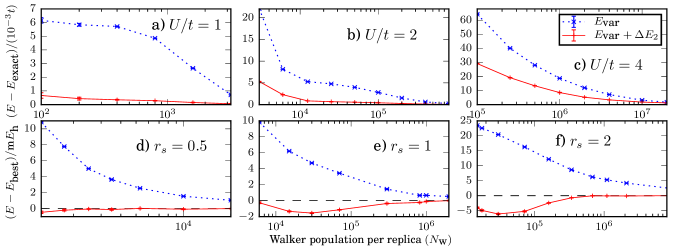
Figure 1: Results for the periodic two-dimensional $18$-site Hubbard model at half-filling (a-c), and the 14-electron spin-unpolarized UEG in three dimensions, with 358 plane-wave spin orbitals (d-f), varying coupling strength ($U/t$ or $r_{s}$) and ${N_{\textrm{w}}}$. For (d-f), dashed lines show near-exact best estimates.

We now discuss the computational cost of this approach. The only additional cost for accumulating $\Delta E_{2}$, compared to basic i-FCIQMC, is in calculating each $H_{aa}$, which is essentially negligible compared to the rest of the simulation. A replica simulation must also be performed, doubling iteration time but also doubling the samples obtained, such that efficiency is unaffected; there is also a doubling of memory, but FCIQMC is significantly more time-limited than memory-limited. There is however a larger cost in calculating the variational energy estimate, $E_{\textrm{var}}$. In our current implementation this is done by first accumulating the FCIQMC two-body reduced density matrix (2-RDM), $\hat{\Gamma}$, as described in Refs. (Overy et al., 2014) and (Blunt, Booth, and Alavi, 2017), with the numerator of the variational energy then obtained as $\textrm{Tr}\big{[}\hat{\Gamma}\hat{H}\big{]}$. Even with the many schemes described previouslyOvery et al. (2014); Blunt, Booth, and Alavi (2017), we currently find that accumulating 2-RDMs increases iteration time by a factor of $\sim 1.5-3$. Such RDM calculations are becoming the norm in FCIQMC, and the cost of calculating $E_{\textrm{var}}$ can likely be reduced, but for now we note this additional cost compared to a non-RDM simulation. Another concern is that $\Delta E_{2}$ may have larger noise than $E_{\textrm{var}}$, and so require additional sampling. Noise in $\Delta E_{2}$ is often larger than in $E_{\textrm{var}}$, but decreases more quickly with walker population, ${N_{\textrm{w}}}$, and we often find that our usual protocol automatically gives sufficiently small error bars in both. However, for some challenging cases far from convergence, additional sampling may be required. Nonetheless, this additional sampling is far cheaper than instead reducing initiator error by increasing ${N_{\textrm{w}}}$ without $\Delta E_{2}$.

Results:- For results, FCIQMC simulations were performed using NECINEC , and SHCI benchmarks obtained using Dice, with integrals generated using PySCFSun et al. (2017). All calculations use time-reversal symmetrized functionsSmeyers and Doreste-Suarez (1973) rather than Slater determinants.

We first apply the correction to the Hubbard model and uniform electron gas (UEG) at a range of coupling strengths. For the Hubbard model we study a periodic two-dimensional 18-site lattice at half-filling, using crystal momentum symmetry ($\bm{K}=\bm{0}$), at $U/t=1$, $2$ and $4$. For the UEG, we take the three-dimensional spin-unpolarized 14-electron system in a basis of 358 plane-wave spin orbitals, again restricting to $\bm{K}=\bm{0}$, and dimensionless density parameters ($r_{s}$) of $0.5$, $1.0$ and $2.0$.

Results are presented in Figure 1 (with data in supplementary material). For the Hubbard model at $U/t=1$ the correction is highly accurate, removing $>90-95\%$ of initiator error for all walker populations considered. With $100$ walkers, for example, initiator error is reduced from $6.2\times 10^{-3}t$ to $0.7\times 10^{-3}t$. At $U/t=2$ the correction is $\sim 75-85\%$. As expected, the correction is less effective at intermediate coupling, though still reducing initiator error from $64\times 10^{-3}t$ to $29\times 10^{-3}t$ with $10^{5}$ walkers.

State	$R$/Å	Benchmark/${E_{\textrm{h}}}$	$E_{\textrm{var}}$/${E_{\textrm{h}}}$	$(E_{\textrm{var}}+\Delta E_{2})$/${E_{\textrm{h}}}$	Initiator error/$\textrm{m}{E_{\textrm{h}}}$	Final error/$\textrm{m}{{E_{\textrm{h}}}}$	% corrected
$X{}^{1}\Sigma_{g}^{{}^{+}}$	1.24253	-75.80271(2)	-75.80071(5)	-75.80272(7)	1.93(5)	-0.01(7)	101(3)
	2.0	-75.64565(2)	-75.64336(4)	-75.6452(1)	2.29(5)	0.4(1)	82(5)
$B^{\prime}{}^{1}\Sigma_{g}^{{}^{+}}$	1.24253	-75.71213(2)	-75.71020(9)	-75.7121(1)	1.80(9)	0.0(1)	98(6)
	2.0	-75.61486(2)	-75.61257(3)	-75.6145(1)	2.29(4)	0.4(1)	82(5)

Table 1: Energies for C₂ in a cc-pVQZ basis set, with 4 core electrons uncorrelated and at equilibrium and stretched geometries. $B^{\prime}{}^{1}\Sigma_{g}^{{}^{+}}$ results use the excited-state FCIQMC algorithmBlunt et al. (2015b). Benchmarks are taken from Ref. (Holmes, Umrigar, and Sharma, 2017), with associated errors marking the stated upper uncertainty. All FCIQMC calculations use $2\times 10^{5}$ walkers per replica and state.

System	Benchmark/${E_{\textrm{h}}}$	${N_{\textrm{w}}}$	$E_{\textrm{var}}$/${E_{\textrm{h}}}$	$(E_{\textrm{var}}+\Delta E_{2})$/${E_{\textrm{h}}}$	Initiator error/$\textrm{m}{E_{\textrm{h}}}$	% corrected
Water (aug-cc-pVDZ)	-76.274457(9)	$1\times 10^{3}$	-76.25901(3)	-76.2750(1)	15.44(3)	104(1)
Ethylene (cc-pVDZ)	-78.35624(2)	$1\times 10^{5}$	-78.35364(2)	-78.3565(1)	2.60(3)	110(5)
Formaldehyde (aug-cc-pVDZ)	-114.2463(1)	$5\times 10^{5}$	-114.24155(2)	-114.2461(2)	4.8(1)	96(4)
Butadiene (ANO-L-pVDZ)	-155.5582(1)	$5\times 10^{7}$	-155.54323(8)	-155.5578(10)	15.0(1)	98(7)

Table 2: Results for molecular systems at the given walker populations, ${N_{\textrm{w}}}$, chosen so that significant initiator error exists. $1s$ cores were frozen in each case. The benchmark for butadiene is a SHCI result from Ref. Chien et al., 2018. Other benchmarks were obtained from new extrapolated SHCI calculations. Results for additional ${N_{\textrm{w}}}$ values are given in supplementary material.

For the UEG at $r_{s}=0.5$, results with the EN2 correction are always correct within $0.5$m${E_{\textrm{h}}}$, and always within $0.1$m${E_{\textrm{h}}}$ for ${N_{\textrm{w}}}\geq 2500$, despite a Hilbert space dimension of $\sim 10^{20}$. For comparison, initiator error is $\approx 5$m${E_{\textrm{h}}}$ at ${N_{\textrm{w}}}=2500$. Although it is not surprising to find a perturbative correction to be effective at low $r_{s}$, this accuracy should address concerns about the validity of the correction within the initiator approximation. Large improvements are again made at $r_{s}=1.0$ and $2.0$, although decreasing somewhat in line with the increasing correlation strength. The results are non-variational here, but even at $r_{s}=2.0$ the correction is $\sim 110-130\%$.

The above UEG example should also address potential concerns about the use of replica sampling in large spaces with small walker populations. Despite a basis of $358$ spin orbitals and as little as $1.25\times 10^{3}$ walkers, error bars in both $E_{\textrm{var}}$ and $\Delta E_{2}$ are well controlled.

In Table 2, carbon dimer results are presented with a cc-pVQZ basis set, with $4$ core electrons uncorrelated, at equilibrium and stretched geometries. We use the excited-state FCIQMC algorithmBlunt et al. (2015b) and study both the ground and first excited states of ${}^{1}\Sigma_{g}^{{}^{+}}$ character. This system has been previously studied with benchmark accuracy by the density matrix renormalization group algorithm (DMRG)Sharma (2015), FCIQMCBlunt et al. (2015b) and SHCIHolmes, Umrigar, and Sharma (2017), and very recently by SharmaSharma (2018) and Guo et al.Guo, Li, and Chan (2018b) in perturbative DMRG studies (although there correlating 12 electrons in a cc-pVDZ basis). In our previous FCIQMC study, it was found that $10^{6}$ walkers were required for an accuracy of $1$m${E_{\textrm{h}}}$ for both states and geometries. With $1.6\times 10^{7}$ walkers, an accuracy of $\sim 0.1-0.2$m${E_{\textrm{h}}}$ was obtained.

Here we consider a much smaller ${N_{\textrm{w}}}$ of $2\times 10^{5}$ to assess $\Delta E_{2}$. At equilibrium geometry, initiator error is around $1.8-1.9$m${E_{\textrm{h}}}$, which is removed effectively in its entirety (within stochastic errors of $0.1$m${E_{\textrm{h}}}$) by the correction. At the more strongly correlated $R=2.0$Å  the correction is slightly less accurate, but still substantial, removing $82\pm 5\%$ of initiator error. The correction is equally effective for the excited $B^{\prime}{}^{1}\Sigma_{g}^{{}^{+}}$ state.

Results are presented in Table 2 for additional molecular systems, with geometries in supplementary materialHoy and Bunker (1979); Schreiber et al. (2008); Daday et al. (2012). The most challenging system here is butadiene in an ANO-L-pVDZ basis, with $22$ electrons correlated in $82$ spatial orbitals, which was previously studied by i-FCIQMCDaday et al. (2012) using $10^{9}$ walkers. Subsequent extrapolated DMRGOlivares-Amaya et al. (2015) and SHCIChien et al. (2018) results agree that the ground-state energy from i-FCIQMC was too high by $\sim 9$m${E_{\textrm{h}}}$, likely due to remaining initiator error, despite the large walker population. Here with a much smaller walker population of $5\times 10^{7}$, almost all initiator error is removed by $\Delta E_{2}$. We note that the error bar on the corrected result is $1$m${E_{\textrm{h}}}$, so it is possible that the true agreement with SHCI is not as accurate as presented. However, even in the event that the quoted value is incorrect by $2$ standard errors, the EN2 correction still represents a dramatic improvement. These calculations did not require careful choice of molecular orbitals, which were always restricted Hartree–Fock orbitals. The computational resources for this study are modest compared to large-scale FCIQMC, using at most $320$ processor cores, while FCIQMC scales efficiently up to at least $10^{4}$ cores, a powerful possibility in combination with the correction presented here.

Conclusion:- We have introduced the calculation of an EN2 correction from discarded spawning attempts in replica i-FCIQMC. The EN2 correction itself is essentially free to accumulate, although some additional cost may be required to accumulate the variational zeroth-order energy estimate, or to perform additional sampling. In non-strongly-correlated cases the correction regularly removes $>90\%$ of initiator error, and even in strongly-correlated regimes represents an important improvement. This correction therefore significantly extends the reach of FCIQMC, which we expect will be a powerful possibility in future applications of the method.

Supplementary Material:- See supplementary material for data from Figure 1, additional results for molecular systems, and discussion of theoretical biases.

I Application to traditional truncated spaces

Ne aug-cc-pVDZ - CAS + EN2
	Wtih an exact $|\Psi_{0}\rangle$			With a stochastic $|\Psi_{0}\rangle$
Active space	$E_{\textrm{CAS}}/{E_{\textrm{h}}}$	$(E_{\textrm{CAS}}+\Delta E_{2})/{E_{\textrm{h}}}$	$\Delta E_{2}/{E_{\textrm{h}}}$	$E_{\textrm{CAS}}/{E_{\textrm{h}}}$	$(E_{\textrm{CAS}}+\Delta E_{2})/{E_{\textrm{h}}}$	$\Delta E_{2}/{E_{\textrm{h}}}$
(8e,8o)	-128.5026265	-128.74429(4)	-0.24167(4)	-128.502625(1)	-128.74430(4)	-0.24168(4)
(8e,13o)	-128.5294242	-128.73796(5)	-0.20854(5)	-128.529427(3)	-128.73798(5)	-0.20855(5)
(8e,16o)	-128.6131153	-128.71468(2)	-0.10156(2)	-128.61312(1)	-128.71469(1)	-0.10157(1)
(8e,17o)	-128.6428048	-128.71299(1)	-0.07018(1)	-128.64280(1)	-128.71299(2)	-0.07019(2)

Table 1: Comparison of CAS calculations wtih EN2 corrections, using FCIQMC as the CAS solver, both with an exact and stochastically-sampled zeroth-order wave function and energy. The system is Ne in an aug-cc-pVDZ basis set with $2$ core electrons uncorrelated, with an FCI energy of $-128.7094755{E_{\textrm{h}}}$. Simulations with an exact zeroth-order wave function use semi-stochastic FCIQMC, but with the deterministic space set to $\mathcal{V}$, such that $E_{\textrm{CAS}}$ is obtained exactly.

As discussed in the main text, as well as correcting initiator error, an FCIQMC-based estimate of $\Delta E_{2}$ may also be applied to standard truncated spaces, such as a complete active space (CAS). This allows a study of the EN2 correction in isolation, without additional complications arising from the unconventional nature of the initiator approximation.

We study such an example here, using FCIQMC to perform CAS calculations (using restricted Hartree–Fock (RHF) orbitals). Instead of removing the closed-shell and virtual orbitals from the simulation, we include them and allow spawning to basis states in which they have non-zero occupation. These spawnings to outside the CAS are then used to construct $\Delta E_{2}$, as described in the main text, and removed from the simulation afterwards.

We study the Ne atom in an aug-cc-pVDZ basis with $2$ uncorrelated core electrons, for which exact FCI may be performed. As well as performing stochastic FCIQMC within the CAS, we also perform a simulation with deterministic application of $\hat{P}$ within $\mathcal{V}$, allowing $|\Psi_{\textrm{CAS}}\rangle$ and $E_{\textrm{CAS}}$ (the zeroth-order wave function and energy) to be obtained exactly. This is done using the semi-stochastic algorithm described in Refs. (Petruzielo et al., 2012) and (Blunt et al., 2015a), but setting the deterministic space to be the entirety of $\mathcal{V}$. Only spawning events outside of $\mathcal{V}$ are allowed, in order to construct $\Delta E_{2}$. In this way, the estimator for $\Delta E_{2}$ has no theoretical bias due to a stochastic zeroth-order energy estimate. This simulation is then compared to one without the semi-stochastic adaptation, where the zeroth-order wave function and energy are both obtained fully stochastically.

Results are presented in Table 1, for active spaces ranging from $(8{\textrm{e}},8{\textrm{o}})$ to $(8{\textrm{e}},17{\textrm{o}})$ (the aug-cc-pVDZ basis has $22$ spatial orbitals in total, after removing the $1s$ core). The results for both the zeroth-order energy estimate and the EN2 correction are identical between simulations with either a stochastic or exact $|\Psi_{\textrm{CAS}}\rangle$, within stochastic error bars of $\sim 10^{-5}{E_{\textrm{h}}}$, demonstrating the efficacy of the approach.

This also allows a comparison of noise in $\Delta E_{2}$ between simulations with different amounts of noise in the zeroth-order estimates. Results with active spaces of $(8{\textrm{e}},8{\textrm{o}})$ and $(8{\textrm{e}},13{\textrm{o}})$ were averaged over exactly $9\times 10^{5}$ iterations, for both stochastic and deterministic cases, allowing direct comparison. For both $(8{\textrm{e}},8{\textrm{o}})$ and $(8{\textrm{e}},13{\textrm{o}})$ active spaces, error bars on estimates of $\Delta E_{2}$ are identical to $1$ significant figure. As such, the use of semi-stochastic within the zeroth-order space does not significantly impact the noise on $\Delta E_{2}$. Studying error bars to a second significant figure shows that results with a deterministic $|\Psi_{\textrm{CAS}}\rangle$ do result in smaller noise on $\Delta E_{2}$, but not substantially so. This is not unreasonable - the number of contributions to $\Delta E_{2}$ is proportional to the square of the number of spawnings outside of $\mathcal{V}$. This density determines the noise on the $\Delta E_{2}$ estimate to a greater extent than the noise on the $|\Psi_{0}\rangle$ estimate.

Likewise, contributions to $\Delta E_{2}$ are not directly correlated from one iteration to the next, but only indirectly through the correlation between $\Psi_{0}(\tau)$ and $\Psi_{0}(\tau+\Delta\tau)$. We find that long autocorrelation lengths are not a significant issue for the sampling of $\Delta E_{2}$, compared to $E_{0}$.

II Data for model systems

We include numerical data for the results of Figure $1$ in the main text, studying the Hubbard model and the uniform electron gas (UEG) at a range of coupling strengths.

For the Hubbard model, an $18$-site periodic two-dimensional lattice is studied at $U/t=1$, $2$ and $4$. The Hilbert space dimension is $\sim 10^{8}$. The time step was kept at a constant value of $\Delta\tau=0.01$ and the initiator threshold was set to $n_{a}=3$. The semi-stochastic adaptation was used at $U/t=4$, with a deterministic space of dimension $10^{4}$, although this is not necessary and does not significantly change either initiator error or $\Delta E_{2}$.

For the UEG, a three-dimensional spin-unpolarized $14$-electron system is studied in a basis of 358 plane-wave spin orbitals, at $r_{s}=0.5$, $1$ and $2$. The Hilbert space dimension here is $\sim 10^{20}$. For $r_{s}=0.5$ a time step of $\Delta\tau=4\times 10^{-4}$ was used. At $r_{s}=1$ and $2$, the time step was varied to prevent creation of large spawning events, resulting in larger time steps of between $\Delta\tau=1\times 10^{-3}$ and $2\times 10^{-3}$, although once again this difference does not significantly alter results, and the EN2 correction is well-behaved regardless.

All calculations use time-reversal symmetrized functionsSmeyers and Doreste-Suarez (1973) rather than Slater determinants.

III Additional data

We present further data for molecular systems at a range of walker populations, ${N_{\textrm{w}}}$. The molecules studied are C₂ in a cc-pVTZ basis (both ground and first excited states of ${}^{1}\Sigma_{g}^{{}^{+}}$ character, at equilibrium and stretched geometries), water in an aug-cc-pVDZ basis, ethylene in a cc-pVDZ basis and formaldehyde in an aug-cc-pVDZ basis. $1s$ cores are uncorrelated in each case.

For water, the semi-stochastic adaptation was not used. For C2, ethylene and formaldehyde, semi-stochastic was used with a deterministic space of dimension $10^{4}$, by picking the most populated basis states upon convergence, as described in Ref. (Blunt et al., 2015a). For butadiene (results presented in the main text), a deterministic space of dimension $2\times 10^{5}$ was used, chosen using the same scheme. Results were typically averaged over between $5\times 10^{4}$ and $10^{6}$ iterations. The initiator threshold was taken as $n_{a}=3$, and the time step was varied in the early stages of the simulation to prevent bloom events (defined as a single spawning event with magnitude greater than $n_{a}$).

Benchmarks for C₂ cc-pVTZ are taken from Ref. (Blunt et al., 2015b). Benchmarks for other systems are obtained from semistochastic heat-bath configuration interaction (SHCI) calculationsHolmes et al. (2016); Sharma et al. (2017) performed with Dice, with quadratic extrapolations as described in Ref. (Chien et al., 2018) (although using RHF orbitals). Time-reversal symmetrized functionsSmeyers and Doreste-Suarez (1973) are used for both FCIQMC and SHCI. For formaldehyde, the smallest threshold for the variational SHCI step was $\epsilon_{\textrm{V}}=10^{-5}$, corresponding to $\sim 3.7\times 10^{7}$ basis states in $\mathcal{V}$. The perturbative threshold was set to $\epsilon_{\textrm{PT}}=10^{-10}$ in all cases.

The geometry for water is from Ref. (Hoy and Bunker, 1979), the geometry for ethylene is taken from Ref. (Schreiber et al., 2008), and the geometry for butadiene is from Ref. (Daday et al., 2012).

$18$-site Hubbard model
${N_{\textrm{w}}}$	$E_{\textrm{var}}/t$	$(E_{\textrm{var}}+\Delta E_{2})/t$	$\Delta E_{2}/(10^{-3}t)$	Initiator error/$(10^{-3}t)$	Final error/$(10^{-3}t)$	% corrected
100	-27.6886(2)	-27.6941(2)	-5.49(7)	6.2(2)	0.7(2)	89(3)
200	-27.6889(1)	-27.6943(1)	-5.40(5)	5.8(1)	0.4(1)	92(2)
400	-27.68900(3)	-27.69437(3)	-5.36(2)	5.72(3)	0.35(3)	93.8(6)
800	-27.68986(1)	-27.69443(2)	-4.572(8)	4.86(1)	0.29(2)	94.1(3)
1600	-27.69206(2)	-27.69456(2)	-2.504(8)	2.66(2)	0.16(2)	94.1(8)
3200	-27.69400(1)	-27.69466(1)	-0.654(5)	0.72(1)	0.06(1)	91(1)
Exact energy/$t$		-27.69472

Table 2: Total energies for the periodic two-dimensional $18$-site Hubbard model at half-filling, at $U/t=1$.

${N_{\textrm{w}}}$	$E_{\textrm{var}}/t$	$(E_{\textrm{var}}+\Delta E_{2})/t$	$\Delta E_{2}/(10^{-3}t)$	Initiator error/$(10^{-3}t)$	Final error/$(10^{-3}t)$	% corrected
$1.5\times 10^{3}$	-23.74375(5)	-23.77703(6)	-33.28(3)	41.65(5)	8.37(6)	79.9(1)
$3\times 10^{3}$	-23.76334(3)	-23.78009(4)	-16.75(2)	22.06(3)	5.31(4)	75.9(1)
$6\times 10^{3}$	-23.77726(2)	-23.78311(2)	-5.85(1)	8.14(2)	2.29(2)	71.9(2)
$1.25\times 10^{4}$	-23.78013(1)	-23.78454(1)	-4.412(5)	5.27(1)	0.86(1)	83.7(2)
$2.5\times 10^{4}$	-23.780632(8)	-23.784725(8)	-4.093(2)	4.771(8)	0.678(8)	85.8(2)
$5\times 10^{4}$	-23.781424(7)	-23.784840(7)	-3.416(1)	3.979(7)	0.563(7)	85.9(2)
$1\times 10^{5}$	-23.782599(7)	-23.784976(7)	-2.3768(7)	2.804(7)	0.427(7)	84.8(2)
$2\times 10^{5}$	-23.783874(8)	-23.785137(8)	-1.2622(5)	1.528(8)	0.266(8)	82.6(4)
$4\times 10^{5}$	-23.784787(9)	-23.785271(9)	-0.4845(4)	0.616(9)	0.132(9)	79(1)
$8\times 10^{5}$	-23.785173(6)	-23.785354(6)	-0.1800(3)	0.229(6)	0.049(6)	78(2)
Exact energy/$t$		-23.78540

Table 3: Total energies for the periodic two-dimensional $18$-site Hubbard model at half-filling, at $U/t=2$.

${N_{\textrm{w}}}$	$E_{\textrm{var}}/t$	$(E_{\textrm{var}}+\Delta E_{2})/t$	$\Delta E_{2}/(10^{-3}t)$	Initiator error/$(10^{-3}t)$	Final error/$(10^{-3}t)$	% corrected
$1\times 10^{5}$	-17.1881(2)	-17.2232(2)	-35.1(2)	64.2(2)	29.1(2)	54.6(3)
$2.5\times 10^{5}$	-17.21235(8)	-17.2332(1)	-20.89(6)	40.04(8)	19.1(1)	52.2(2)
$5\times 10^{5}$	-17.22437(6)	-17.23901(7)	-14.63(3)	28.01(6)	13.38(7)	52.2(2)
$1\times 10^{6}$	-17.2337(1)	-17.2438(1)	-10.12(5)	18.7(1)	8.6(2)	54.1(5)
$2\times 10^{6}$	-17.24045(5)	-17.24712(5)	-6.67(2)	11.93(5)	5.27(5)	55.9(3)
$4\times 10^{6}$	-17.24524(4)	-17.24900(4)	-3.76(1)	7.14(4)	3.38(4)	52.6(4)
$1\times 10^{7}$	-17.24925(4)	-17.25058(4)	-1.322(7)	3.13(4)	1.81(4)	42.2(6)
$2\times 10^{7}$	-17.25065(4)	-17.25116(4)	-0.515(4)	1.74(4)	1.22(4)	29.6(8)
Exact energy/$t$		-17.25239

Table 4: Total energies for the periodic two-dimensional $18$-site Hubbard model at half-filling, at $U/t=4$.

Uniform electron gas
${N_{\textrm{w}}}$	$E_{\textrm{var}}/{E_{\textrm{h}}}$	$(E_{\textrm{var}}+\Delta E_{2})/{E_{\textrm{h}}}$	$\Delta E_{2}/\textrm{m}{E_{\textrm{h}}}$	Initiator error/$\textrm{m}{E_{\textrm{h}}}$	Final error/$\textrm{m}{{E_{\textrm{h}}}}$	% corrected
1250	-0.56906(7)	-0.5804(1)	-11.3(1)	10.85(7)	-0.5(2)	104(1)
1750	-0.57212(5)	-0.5801(1)	-7.98(10)	7.79(6)	-0.2(1)	103(1)
2500	-0.57490(3)	-0.57996(5)	-5.06(4)	5.01(4)	-0.05(6)	101(1)
3500	-0.57626(6)	-0.58002(9)	-3.76(8)	3.65(7)	-0.11(10)	103(3)
5300	-0.57736(3)	-0.57989(4)	-2.53(3)	2.55(4)	0.02(5)	99(2)
10000	-0.57836(5)	-0.57998(6)	-1.63(3)	1.55(6)	-0.07(7)	105(5)
20000	-0.57887(3)	-0.57991(3)	-1.04(1)	-	-	-
Best estimate/${E_{\textrm{h}}}$		-0.57991(3)

Table 5: Correlation energies for the 14-electron UEG in three dimensions, in a basis of 358 plane-wave spin orbitals, at $r_{s}=0.5$. The benchmark is taken from the largest ${N_{\textrm{w}}}$ considered, although we note that an i-FCIQMC value of $-0.5798(3){E_{\textrm{h}}}$ from Ref. (Neufeld and Thom, 2017) is within error bars.

${N_{\textrm{w}}}$	$E_{\textrm{var}}/{E_{\textrm{h}}}$	$(E_{\textrm{var}}+\Delta E_{2})/{E_{\textrm{h}}}$	$\Delta E_{2}/\textrm{m}{E_{\textrm{h}}}$	Initiator error/$\textrm{m}{E_{\textrm{h}}}$	Final error/$\textrm{m}{{E_{\textrm{h}}}}$	% corrected
$6\times 10^{3}$	-0.50887(4)	-0.5190(1)	-10.1(1)	9.85(6)	-0.3(1)	103(1)
$1.5\times 10^{4}$	-0.51252(3)	-0.52007(6)	-7.55(5)	6.20(6)	-1.34(8)	122(1)
$3\times 10^{4}$	-0.51400(3)	-0.52028(5)	-6.28(4)	4.72(6)	-1.56(7)	133(2)
$7\times 10^{4}$	-0.51528(3)	-0.51987(4)	-4.59(2)	3.44(6)	-1.14(6)	133(2)
$3\times 10^{5}$	-0.51728(4)	-0.51908(5)	-1.80(1)	1.44(7)	-0.36(7)	125(6)
$8.2\times 10^{5}$	-0.51806(5)	-0.51895(5)	-0.891(7)	0.66(7)	-0.23(7)	135(15)
$1\times 10^{6}$	-0.51806(4)	-0.51883(4)	-0.776(7)	0.67(6)	-0.11(6)	116(11)
$2\times 10^{6}$	-0.51820(5)	-0.51872(5)	-0.522(3)	-	-	-
Best estimate/${E_{\textrm{h}}}$		-0.51872(5)

Table 6: Correlation energies for the 14-electron UEG in three dimensions, in a basis of 358 plane-wave spin orbitals, at $r_{s}=1.0$. The benchmark is taken from the largest ${N_{\textrm{w}}}$ considered, although we note an i-FCIQMC value of $-0.51880(2){E_{\textrm{h}}}$ from Ref. (Neufeld and Thom, 2017), showing good agreement.

${N_{\textrm{w}}}$	$E_{\textrm{var}}/{E_{\textrm{h}}}$	$(E_{\textrm{var}}+\Delta E_{2})/{E_{\textrm{h}}}$	$\Delta E_{2}/\textrm{m}{E_{\textrm{h}}}$	Initiator error/$\textrm{m}{E_{\textrm{h}}}$	Final error/$\textrm{m}{{E_{\textrm{h}}}}$	% corrected
$1.5\times 10^{4}$	-0.41211(5)	-0.4396(2)	-27.5(2)	23.48(7)	-4.0(2)	117(1)
$1.75\times 10^{4}$	-0.41300(5)	-0.4405(2)	-27.5(2)	22.59(8)	-4.9(3)	122(1)
$3\times 10^{4}$	-0.41515(5)	-0.4417(2)	-26.6(2)	20.43(8)	-6.1(2)	130(1)
$7.2\times 10^{4}$	-0.41931(9)	-0.4408(2)	-21.5(2)	16.3(1)	-5.2(2)	132(1)
$1.6\times 10^{5}$	-0.42340(5)	-0.43801(10)	-14.61(8)	12.18(8)	-2.4(1)	120(1)
$3.4\times 10^{5}$	-0.42694(5)	-0.43631(7)	-9.36(6)	8.64(8)	-0.72(10)	108(1)
$6.8\times 10^{5}$	-0.42934(5)	-0.43563(8)	-6.29(6)	6.25(8)	-0.05(10)	101(2)
$1.1\times 10^{6}$	-0.43030(6)	-0.43566(5)	-5.36(3)	5.29(8)	-0.07(8)	101(2)
$2.1\times 10^{6}$	-0.43138(6)	-0.43569(6)	-4.31(3)	4.20(9)	-0.11(9)	103(2)
$8.9\times 10^{6}$	-0.43314(5)	-0.43558(6)	-2.45(1)	-	-	-
Best estimate/${E_{\textrm{h}}}$		-0.435584(58)

Table 7: Correlation energies for the 14-electron UEG in three dimensions, in a basis of 358 plane-wave spin orbitals, at $r_{s}=2.0$. The benchmark is taken from the largest ${N_{\textrm{w}}}$ considered, ${N_{\textrm{w}}}=8.9\times 10^{6}$. We could not find independent i-FCIQMC results for comparison, although stochastic coupled cluster results for CCSD and CCSDT from Ref. (Neufeld and Thom, 2017) are -0.40181(4)${E_{\textrm{h}}}$ and -0.43212(7)${E_{\textrm{h}}}$, respectively.

C2 cc-pVTZ
State	$R$/Å	Best estimate/${E_{\textrm{h}}}$	$E_{\textrm{var}}$/${E_{\textrm{h}}}$	$(E_{\textrm{var}}+\Delta E_{2})$/${E_{\textrm{h}}}$	Initiator error/$\textrm{m}{E_{\textrm{h}}}$	Final error/$\textrm{m}{{E_{\textrm{h}}}}$	% corrected
$X{}^{1}\Sigma_{g}^{{}^{+}}$	1.25	-75.78515(10)	-75.78382(1)	-75.78519(3)	1.3(1)	0.0(1)	103(8)
	2.0	-75.63095(10)	-75.62939(3)	-75.63087(5)	1.6(1)	0.1(1)	95(8)
$B^{\prime}{}^{1}\Sigma_{g}^{{}^{+}}$	1.25	-75.69572(10)	-75.69455(2)	-75.69578(4)	1.2(1)	0.1(1)	105(9)
	2.0	-75.60145(10)	-75.59996(3)	-75.60138(6)	1.5(1)	0.1(1)	96(8)

Table 8: Energies for the carbon dimer in a cc-pVTZ basis set, with 4 core electrons uncorrelated, at equilibrium and stretched geometries. $B^{\prime}{}^{1}\Sigma_{g}^{{}^{+}}$ results use the excited-state FCIQMC algorithm. Best estimates are taken from Ref. (Blunt et al., 2015b). All FCIQMC calculations use $1\times 10^{5}$ walkers per replica and state.

Water aug-cc-pVDZ
${N_{\textrm{w}}}$	$E_{\textrm{var}}/{E_{\textrm{h}}}$	$(E_{\textrm{var}}+\Delta E_{2})/{E_{\textrm{h}}}$	$\Delta E_{2}/\textrm{m}{E_{\textrm{h}}}$	Initiator error/$\textrm{m}{E_{\textrm{h}}}$	Final error/$\textrm{m}{{E_{\textrm{h}}}}$	% corrected
$1\times 10^{3}$	-76.25901(3)	-76.2750(1)	-16.0(2)	15.44(3)	-0.6(2)	104(1)
$1\times 10^{4}$	-76.27024(2)	-76.27393(6)	-3.69(5)	4.22(2)	0.53(6)	87(1)
$4\times 10^{4}$	-76.27306(2)	-76.27439(4)	-1.33(4)	1.40(2)	0.07(4)	95(3)
$8\times 10^{4}$	-76.27357(2)	-76.27447(3)	-0.90(2)	0.89(2)	-0.01(4)	101(4)
$1.6\times 10^{5}$	-76.27383(2)	-76.27446(2)	-0.636(9)	0.63(2)	-0.01(2)	101(4)
Benchmark energy/${E_{\textrm{h}}}$		-76.274457(9)

Table 9: Energies for the water molecule at equilibrium geometry in the aug-cc-pVDZ basis set. The benchmark energy is obtained from SHCI calculations with a (very small) extrapolation.

Ethylene cc-pVDZ
${N_{\textrm{w}}}$	$E_{\textrm{var}}/{E_{\textrm{h}}}$	$(E_{\textrm{var}}+\Delta E_{2})/{E_{\textrm{h}}}$	$\Delta E_{2}/\textrm{m}{E_{\textrm{h}}}$	Initiator error/$\textrm{m}{E_{\textrm{h}}}$	Final error/$\textrm{m}{{E_{\textrm{h}}}}$	% corrected
$1\times 10^{5}$	-78.35364(2)	-78.3565(1)	-2.8(1)	2.60(3)	-0.2(1)	110(5)
$2.5\times 10^{5}$	-78.35409(2)	-78.35639(6)	-2.30(6)	2.15(3)	-0.15(6)	107(3)
$5\times 10^{5}$	-78.35440(1)	-78.35635(3)	-1.95(3)	1.84(2)	-0.11(3)	106(2)
$5\times 10^{6}$	-78.35561(1)	-78.35622(1)	-0.615(5)	0.63(2)	0.02(2)	97(4)
$1\times 10^{7}$	-78.355832(7)	-78.356227(6)	-0.394(3)	0.41(2)	0.01(2)	97(5)
Benchmark energy/${E_{\textrm{h}}}$		-78.35624(2)

Table 10: Energies for the ethylene molecule at equilibrium geometry in the cc-pVDZ basis set. The benchmark energy is obtained from SHCI calculations with a (very small) extrapolation.

Formaldehyde aug-cc-pVDZ
${N_{\textrm{w}}}$	$E_{\textrm{var}}/{E_{\textrm{h}}}$	$(E_{\textrm{var}}+\Delta E_{2})/{E_{\textrm{h}}}$	$\Delta E_{2}/\textrm{m}{E_{\textrm{h}}}$	Initiator error/$\textrm{m}{E_{\textrm{h}}}$	Final error/$\textrm{m}{{E_{\textrm{h}}}}$	% corrected
$5\times 10^{5}$	-114.24155(2)	-114.2461(2)	-4.6(2)	4.8(1)	0.2(2)	96(4)
$1\times 10^{6}$	-114.24244(2)	-114.2462(1)	-3.8(1)	3.9(1)	0.1(2)	97(4)
$2\times 10^{6}$	-114.24316(2)	-114.24604(7)	-2.88(7)	3.1(1)	0.3(1)	92(4)
$4\times 10^{6}$	-114.24374(1)	-114.24612(3)	-2.37(3)	2.6(1)	0.2(1)	93(4)
Best estimate/${E_{\textrm{h}}}$		-114.2463(1)

Table 11: Energies for the formaldehyde molecule at equilibrium geometry in the aug-cc-pVDZ basis set. The benchmark energy is obtained from SHCI calculations with an extrapolation.

Geometries (Å)

Water
O	0.0000	0.0000	0.1173
H	0.0000	0.7572	-0.4692
H	0.0000	-0.7572	-0.4692

Ethylene
H	0.000000	0.923274	1.238289
H	0.000000	-0.923274	1.238289
H	0.000000	0.923274	-1.238289
H	0.000000	-0.923274	-1.238289
C	0.000000	0.000000	0.668188
C	0.000000	0.000000	-0.668188

Formaldehyde
O	0.000000	0.0000	1.2050
C	0.000000	0.0000	0.0000
H	0.000000	0.9429	-0.5876
H	0.000000	-0.9429	-0.5876

Butadiene
C	0.000000	1.834350	-0.157794
C	0.000000	-1.834350	0.157794
C	0.000000	0.612753	0.388232
C	0.000000	-0.612753	-0.388232
H	0.000000	0.509700	1.466975
H	0.000000	-0.509700	-1.466975
H	0.000000	2.723649	0.452738
H	0.000000	-2.723649	-0.452738
H	0.000000	1.961466	-1.231090
H	0.000000	-1.961466	1.231090

References

- Petruzielo et al. (2012) F. R. Petruzielo, A. A. Holmes, H. J. Changlani, M. P. Nightingale, and C. J. Umrigar, Phys. Rev. Lett. 109, 230201 (2012).
- Blunt et al. (2015a) N. S. Blunt, S. D. Smart, J. A. F. Kersten, J. S. Spencer, G. H. Booth, and A. Alavi, J. Chem. Phys. 142, 184107 (2015a).
- Smeyers and Doreste-Suarez (1973) Y. G. Smeyers and L. Doreste-Suarez, Int. J. Quantum Chem. 7, 687 (1973).
- Blunt et al. (2015b) N. S. Blunt, S. D. Smart, G. H. Booth, and A. Alavi, J. Chem. Phys. 143, 134117 (2015b).
- Holmes et al. (2016) A. A. Holmes, N. M. Tubman, and C. J. Umrigar, J. Chem. Theory Comput. 12, 3674 (2016).
- Sharma et al. (2017) S. Sharma, A. A. Holmes, G. Jeanmairet, A. Alavi, and C. J. Umrigar, J. Chem. Theory Comput. 13, 1595 (2017).
- Chien et al. (2018) A. D. Chien, A. A. Holmes, M. Otten, C. J. Umrigar, S. Sharma, and P. M. Zimmerman, J. Phys. Chem. A 122, 2714 (2018).
- Hoy and Bunker (1979) A. R. Hoy and P. R. Bunker, J. Mol. Spectrosc. 74, 1 (1979).
- Schreiber et al. (2008) M. Schreiber, M. R. Silva-Junior, S. P. A. Sauer, and W. Thiel, J. Chem. Phys. 128, 134110 (2008).
- Daday et al. (2012) C. Daday, S. Smart, G. H. Booth, A. Alavi, and C. Filippi, J. Chem. Theory Comput. 8, 4441 (2012).
- Neufeld and Thom (2017) V. A. Neufeld and A. J. W. Thom, J. Chem. Phys. 147, 194105 (2017).