Recovery of spectrum from estimated covariance matrices and statistical kernels for machine learning and big data

Abstract

Let $X$ be a $n\times p$ random matrix with independent rows all distributed as the random vector $\vec{X}=(X_{1},X_{2},\ldots,X_{p})$ and having $0$ expectation. The sample covariance matrix is then defined by $\widehat{COV}[\vec{X}]=X^{t}X/n$ and is the maximum likelihood estimate of the covariance matrix $COV[\vec{X}]$ when the data is normal. We are interested in the regime where $n$ and $p$ both go to infinity at the same time so that $n/p$ converges to a non-zero number $\alpha>0$. In that case, the spectrum of the sample covariance converges to the free product of $\mu$ with a Marchenko-Pastur distribution [17], provided the spectrum of the covariance converges to $\mu$. In theory, from the limiting distribution of the estimated covariance matrix, one could retrieve $\mu$ using the $S$-transform from free probability.

In many practical applications, the spectrum of the “actual” covariance contains essential information about the structure of the data at hand. There is a family of spectrum-reconstruction-algorithms, which attempt to discretize and adapt the free probability infinite-dimensional-recovery. This approach, pioneered by EI Karoui [5], was further developed by Silverstein [18], Bai and Yin [1], Yin, Bai and Krishnaiah [22] and recently Ledoit and Wolf [12], [16] and [13]. There is also the shrinkage method pioneered by Stein [19], see also Bickel and Levina [3] and Donoho [7]. Another type of approach is based on the moments of the spectral distributions see for example Kong and Valliant [11]. This can be very useful as parallel method. Finally, there are also Physicists Burda, Görlich and Jarosz, working on this problem [4].

We present a simple algebraic formula (1.10) for reconstructing the spectrum of the covariance matrix given only the sample covariance spectrum. For normal data with $n/p\geq 2$ and the spectrum taken from real data, this approximation allows to recover the true underlying spectrum quite closely (See Figure 3). For spectrum which is too flat however it does not work well (See Figure 9).

We also introduce a second algorithm which is a fixed point method, with remarkable reconstruction of the spectrum when $n/p\geq 1$ in both simulated and real data. For this, we take real life data with $n$ much bigger than $p$ to estimated the “true covariance”’s spectrum. Then, we compare it to our reconstruction using a small subset of the real-life data for which $n/p$ is much smaller. (See Figure 4, where $n/p=1$).

Finally we present a proof of concept for big data, by showing that our method applied to a reduced real life data set, allows to recover almost perfectly the underlying spectrum of the full-data set. (See Figure 10). Our method does not seem to work well on sparse data, though this is not our main focus in this note.

Our first approximation is derived in a purely probabilistic way using the formula for the spectral norm of error matrix [10] by Koltchinskii and Lounici.

1 Introduction

1.1 The setup

We consider a random matrix $Z$ of dimension $n\times p$ which represents some data. We will be primarily interested in the eigenvectors of the expected matrix $E[Z^{t}Z]$ called Principal Components. The principal components corresponding to the highest eigenvalues, often carry some structural information about the underlying data. Instead of being given the expected matrix, only $Z^{t}Z$ is usually observable. We will take the eigenvectors of $Z^{t}Z$ and hope they approximate the eigenvectors of $E[Z^{t}Z]$ well. This is the setting for covariance matrix analysis via principal components, as well as analysis of statistical kernels via principal components.

For example, when the rows of $Z$ have $0$ expectation and are i.i.d., the expectation of $Z^{t}Z/n$ corresponds to the covariance matrix

$$COV(\vec{Z})=E[\frac{Z^{t}Z}{n}].$$ (1.1)

where $\vec{Z}$ has the distribution of a row of $Z$. In this case of i.i.d. rows with $0$ expectation, the sample covariance matrix is given

$$\widehat{COV}[\vec{Z}]:=\frac{Z^{t}Z}{n}.$$ (1.2)

It is an unbiased maximum-likelihood estimator of the true covariance matrix when the data is normal.

In this paper, we present two new algorithms which allow in many practical situations to get very close to retrieving the spectrum of $E[Z^{t}Z]$ given only the spectrum of $Z^{t}Z$. Our algorithms to our knowledge allow a level of precision with most real-life data which is remarkable. Our reconstruction of the real spectrum is often precise enough to determine details of the spectrum of $E[Z^{t}Z]$ like for example “elbows”.

Let $X$ be a $n\times p$ matrix with i.i.d. multivariate standard normal random variables. The sample covariance matrix is then defined by $\widehat{COV}[{X}]=\frac{1}{n}X^{t}X$ and is a maximum-likelihood estimate of the covariance matrix $COV[{X}]$, which is identity. We are interested in the high dimensional setting, where $n$ and $p$ both go to infinity at the same time so that $\frac{p}{n}$ converges to a non-zero fixed limit. In 1967, Vladimir Marčenko and Leonid Pastur [17] successfully constructed the limiting law, which is now named after the authors.

For the case of $COV[{X}]$ is not identity, we assume its spectrum admits a limiting law $F^{\Sigma}$. Then sample spectrum is a free product of Marčenko-Pastur law and $F^{\Sigma}$. By computing the $S$-transform explicitly, one can obtain a formula of the limiting law of the sample spectrum as for instance discussed in Bai and Yin [1], Yin, Bai and Krishnaiah [22], Silverstein [18], and many others. The main result is summarized as follows.

Theorem 1.1.

Assume the following.

1. The entries of $X_{p}=(X_{i,j})_{n\times p}$ are i.i.d. real random variables for all $p$.

2. $E[X_{1,1}]=0$, $E[|X_{1,1}|^{2}]=1$.

3. Let $p/n\to c>0$ as $p\to\infty$.

4. Let $\Sigma_{p}$ $(p\times p)$ be non-negative definite symmetric random matrix with spectrum distribution $F^{\Sigma_{p}}$ (If $\{\lambda_{i}\}_{1\leq i\leq p}$ are the eigenvalues of $\Sigma_{p}$, then $F^{\Sigma_{p}}=\sum_{1}^{p}\frac{1}{p}\delta_{\lambda_{i}}(x)$) such that $F^{\Sigma_{p}}$ almost surely converges weakly to $F^{\Sigma}$ on $[0,\infty)$.

5. $X_{p}$ and ${\Sigma}_{p}$ are independent.

Then the spectrum distribution of $W_{p}=\frac{1}{n}{\Sigma}_{p}^{1/2}X_{p}^{T}X_{p}{\Sigma}_{p}^{1/2}$, denoted as $F^{W_{p}}$ almost surely converges weakly to $F^{W}$. $F^{W}$ is the unique probability measure whose Stieltjes transform $m(z)=\int\frac{dF^{W}(x)}{x-z}$, $z\in\mathbb{C}^{+}$ satisfies the equation

$$-\frac{1}{m}=z-c\int\frac{t}{1+tm}dF^{\Sigma}(t)\quad\forall z\in\mathbb{C}^{+}$$ (1.3)

In many real life application, the spectrum of the true covariance matrix contains essential information about the underlying structure of the data. Now, this is not the spectrum of the estimated covariance if there is a big difference. For example if $n=p/2$, then the estimated covariance matrix is defective and has at least half of its eigenvalues equal to $0$. In financial analysis, a concrete example is the daily stock returns. The spectrum of the underlying covariance matrix are bounded away from $0$ by a term of order $O(1)$, since stocks are not linearly dependent. Thus spectrum of the defective sample covariance matrix “makes” an error of order at least $O(1)$.

One important approach is using the free probability results and attempts at solving the equation (1.3) to get an estimator of the true spectrum $F^{\Sigma}$. First such work is due to EI Karoui [5], and then Bai etc. [2], and recently by Ledoit and Wolf [12], [16] and [13]. It’s not surprising that as dimensions grow, consistency is achieved in theory, by the free probability approach. We say “in theory”, because for real-life-data there are usually some eigenvalues of the spectrum which are of order $O(p)$ and others of order $O(1)$, so that the spectrum of the underlying covariance matrix does not converge to a limit. Furthermore, a disadvantage of the free-probability approach is that the recovered spectrum can still be far from the true spectrum for small or moderate size of $p$.

1.2 Our results

In the current paper, we first present a simple algebraic formula (1.11) for the sample eigenvalues which approximates the true covariance eigenvalues. For normal data, this approximation is quite efficient and gives quite good corrections as soon as $n/p\geq 2$ and the true spectrum is not too flat (see for instance Figure 3). In addition to this we present a more precise recovery, we introduce a fixed point iteration method. This method uses the matrix of the eigenvectors of the true covariance matrix expressed in the basis of the eigenvectors of the sample covariance.

The second algorithm is more costly but can reconstruct almost perfectly if the true spectrum is not too wild. Our methods are also applied to real data which turns out to work very well as long as the data at hand is not sparse.

Our formula (1.10) leading to first approximation, looks similar to the $S$-transform from free probability and thus resembles the free probability approach. Nonetheless, we derived it in a purely probabilistic way using the formula for the size of the norm of the error matrix of covariance [10] proven by Koltchinskii and Lounici. Our method is the only one which, to our knowledge, is often precise enough to allow to detect important features such as “elbows” in the spectrum of real data. Our formula (1.10) for approximating the difference in spectrum between sample covariance and true covariance, could be written with the distribution function in a similar way to (1.3) as follows

$$-\int\frac{y}{y-invF^{W_{p}}(x)}dF^{W_{p}}(y)\approx\frac{invF^{W_{p}}(x)}{invF^{\Sigma_{p}}(x)}-1,$$ (1.4)

for $x\in[0,1]$. Here $invF(.)$ designates the inverse of the distribution function $F(.)$. Also, when $p$ is finite, then the integral on the right side of (1.4) is an integration with respect to a discrete measure, and one needs to leave out $y=invF^{W_{p}}(x)$ (and even $3$ to $5$ $y$’s closest to $invF^{W_{p}}(x)$) for the formula to work. At the limit, the right side of (1.4) is an improper integral. Now, the difference between the free probability approach and ours is that though for many real life situations, our formula (1.4) is very precise, we don’t expect it to converge to an exact solution as $p$ goes to infinity. In other words, as $p$ goes to infinity, (1.4) should not become an exact equation, but should remain an approximation.

In Subsection (2.1), we show how the approximation (1.10) is derived, without providing a rigorous bound for the error of that approximation. We just note that for practical purposes, the approximation (1.10) seems quite good.

Our second spectrum reconstruction algorithm is a fixed point method. We present it in Subsection 2.2. There we introduce a map (2.22) defined with the help of the sample covariance spectrum and related to the matrix of the second moments of the coefficients for the eigenvectors. That is, the eigenvectors of the true covariance matrix expressed in the basis of the eigenvectors of the sample covariance matrix. The map (2.22) can be applied to any spectrum, but is defined with the help of the sample covariance. In Subsection 2.2, we show that for this map and up to a smaller order term, the spectrum of the true covariance matrix is a fixed point. We prove nothing else, but for practitioners this is already very valuable. Indeed, a continuous map from a compact space into itself could be chaotic, periodic or have fixed points. We know from practice that our map is not chaotic nor periodic, so it must have fixed points. Hopefully, in the terminology of dynamical systems, this fixed point is an attractor and this would explain why we have this great convergence, however we do not have a proof of this results yet. Hence, the main problem would be that we converge to a wrong fixed point, (i.e. not to the desired spectrum of the true covariance). In practice this is not happening, except if the true spectrum is very flat or if $n/p$ is quite smaller than say about $0.5$. On top of it, we can use our first method to find a good enough starting point for the eigenvalues fixed point method. The fixed point algorithm presented in Subsection 2.2 consists then simply in applying the map (2.22) until it stabilizes. In many examples, one iteration of (2.22) is enough to get a good approximation of the spectrum of the true covariance matrix. (See Figure 3) One way of looking at this approximation is that the difference of the sample spectrum to true spectrum can be viewed as a kind of moving average. This sort of moving average of the sample spectrum involve some weights of the moving average which gradually modify as we change location. These weights are then given by the columns of a matrix $B(\widehat{\lambda}_{1},\widehat{\lambda}_{2},\ldots,\widehat{\lambda}_{p})$, where $B(.)$ is the matrix defined in (2.20). From this point of view, our formulas have one very important advantage. Namely, they give a simple intuitive explanation of how approximately the spectrum of the covariance gradually changes into the sample covariance. In contrast, the free probability approach is based on algebraic properties which is convoluted enough and to our best knowledge alludes an intuitive explanation of what the transform “does” to the spectrum of the covariance. On the other hand, the free probability approach from a theoretical point of view, has an advantage, namely, one can prove convergence when $p$ goes to infinity when the spectrum of true covariance converges. (But, that spectrum does not converge in measure since some eigenvalues are of order $O(1)$ whilst others are $O(p)$ for real-life-data). Furthermore, a practitioner might argue that since we have proven the spectrum of the true covariance to be a fixed point of our map (2.22) (up to a smaller order term), even for finite $p$ we can get very good approximations of the true spectrum. We will study more mathematical properties of the map (2.22) in an upcoming paper which will put on solid grounds this approach.

1.3 Examples of $Z^{t}Z$ and their applications for machine learning

Think of $Z$ as a matrix where each column represents a point in $\mathbb{R}^{n}$ and that we have a machine learning problem concerning these points. Note that most machine learning algorithms depend only on the relative position of the input data-points to each other. If we know all the scalar products between the vectors representing the data-points, then we know the relative positions of the points to each other. This is so because we can then determine the angles between the vectors representing these points and also their length. Thus, if the columns of $Z$ represent the data-points we want to use for a machine learning problem, then $Z^{t}Z$ gives all the scalar products between the vectors representing these points. Consequently, $Z^{t}Z$ defines in a unique way the relative position of the points to each other. Most machine learning algorithms depend only on the relative position of input-points to each other, and hence only on $Z^{t}Z$. This shows why most machine learning algorithms can be thought of as having as input a matrix $Z^{t}Z$, where the columns of $Z$ represent the data-points for the machine learning task at hand.

Now, one of the first things practitioners who look at a new data set do is to consider the spectrum of $Z^{t}Z$. In reality however, they would be more interested in the spectrum of $E[Z^{t}Z]$ and with very large feature space and not that large sample size, the difference can be big. That is, the difference between the spectrum of $Z^{t}Z$ and the spectrum of $E[Z^{t}Z]$ is not negligible when $n$ is not much larger than $p$.

Let us give an example of a kernel for document classification, in order to explain why the spectrum of the $Z^{t}Z$ is of interest to practitioners.

Example 1.1.

Consider that we have a collection of short documents $D_{1},D_{2},\ldots,D_{n}$. Let $w_{1},w_{2},\ldots,w_{p}$ be a sequence of non-random words, which occur in our documents. Take $Z$ to be the $n\times p$ matrix, whose $ij$-th entry is $1$ if the $j$-th word occurs in the $i$-th document and $0$ otherwise. The matrix $Z^{t}Z$ has then as $ij$-entry the number of documents where the words $w_{i}$ and $w_{j}$ co-occur. Let $\vec{p}$ and $\vec{q}$ be two probability distributions over the set of words. This simply means that $\vec{p}$ and $\vec{q}$ both have length $p$ and have non-negative entries which sum up to one. Assume that every documents gets randomly labeled as topic 1 or topic 2 document. We can generate every document as a sequence of i.i.d. words, drawn from either the topic 1 or topic 2 distribution depending on the topic classification of the document. We describe here a simple way to think about how the documents where generated by a random process. Let $m$ be the number of words in each document. Assuming $m$ is not too large, we get the approximation

$$E[Z^{t}Z]\approx n\cdot m\left(\;(m-1)(P(T_{1})\cdot\vec{p}\otimes\vec{p}+P(T_{2})\cdot\vec{q}\otimes\vec{q})+diag(P(T_{1})\cdot\vec{p}+P(T_{2})\cdot\vec{q})\;\right)$$ (1.5)

Where $diag(\vec{x})$ represents the diagonal $p\times p$-matrix having on the diagonal the vector $\vec{x}\in\mathbb{R}^{p}$ and $T_{1}$, resp. $T_{2}$ designates the first, respectively the second topic.

Note that the matrix $\vec{p}\otimes\vec{p}$, respectively $\vec{q}\otimes\vec{q}$ has as unique non-zero eigenvalue $|\vec{p}|^{2}$, resp $|\vec{q}|^{2}$. Let $\vec{p}=(p_{1},p_{2},\ldots,p_{p})$, then

$$\max_{i}p_{i}\geq|\vec{p}|^{2}\geq\min_{i}p_{i}.$$

and similarly

$$\max_{i}q_{i}\geq|\vec{q}|^{2}\geq\min_{i}q_{i}.$$

Thus, the matrix $E[Z^{t}Z]$ is up to linear factor a sum of the two terms. The first one

$$(m-1)\left(P(T_{1})\cdot\vec{p}\otimes\vec{p}+P(T_{2})\cdot\vec{q}\otimes\vec{q}\right)$$ (1.6)

and the second one is the diagonal matrix

$$diag(P(T_{1})\cdot\vec{p}+P(T_{2})\cdot\vec{q}).$$ (1.7)

As soon as $m$ is not too small, the eigenvalues of (1.6) will dominate the ones of (1.7) due to the factor $(m-1)$. Here, we have two topics only, but in a realistic model with $k$ topics and $m$ not too large we should see $k$ eigenvalues of order $O(nm^{2}|\vec{p}_{j}|^{2})$ corresponding to the $k$ topics for $j=1,2,\ldots,k$ and the rest of the eigenvalues will roughly correspond to the probabilities in the probability vector for the words times $nm$. Here $\vec{p}_{j}$ designated the probability distribution of the words, given the $j$-th topic which we call $T_{j}$. Thus, under this model, the spectrum of the covariance matrix will contain $k$-higher order eigenvalues corresponding to the topics and the rest of the eigenvalues will be of order $O(1)$, so in the spectrum of the matrix $E[Z^{t}Z]$ we expect to see an “elbow” at the $k$-th eigenvalue. Ideally, for real data, looking at the spectrum should tell us how many topics there are, more precisely this should be quantified by the “elbow” which tells us where the top eigenvalues start detaching from the rest of spectrum. Now often you don’t see an elbow in the spectrum of $Z^{t}Z$ although there might be one in $E[Z^{t}Z]$, the reason being, that the spectrum of $Z^{t}Z$ can be considered a smoothing of the spectrum of $E[Z^{t}Z]$.

The previous example is mainly here to show how the spectrum of $E[Z^{t}Z]$ is important in most machine learning problems. This is not the first situation we encountered. We started working on the reconstruction of the ground-truth spectrum in the context of financial data that is not too far from multidimensional normal distribution. It is true that for short documents, the matrix $Z^{t}Z$ of the previous example is sparse. Our method, of spectrum reconstruction does not yet work on sparse data.

With real data, often the spectrum of the estimated covariance matrix, $Z^{t}Z$ has little fluctuation in it, but a big bias, due to the concentration of measure phenomena. Thus this spectrum can be considered almost as a non-random function of the spectrum of the true covariance matrix. If this “almost non-random map” is injective it would be possible to reconstruct almost exactly the true spectrum from the estimated one, at least assuming that the data is multivariate normal.

Let us give another example. This is the example of stocks, which is pedagogically a very good example although it is not where PCA is necessarily most useful. Indeed, for stocks, the sectors and the capitalization are factors which are known and for which we do not need PCA to discover them.

Example 1.2.

Let $\vec{Z}=(Z_{1},Z_{2},\ldots,Z_{p})$ be a random vector with $0$ expectation and multivariate normal probability distribution. Let $Z$ be $n$ times $p$ matrix where $Z_{ij}$ is the daily return on day $i$ of the $j$-th stock in a given portfolio. Hence we have $p$ stocks and $n$ days considered. Let us denote by $\vec{Z}_{i}$ the $i$-th row of $Z$. We assume that $\vec{Z},\vec{Z}_{1},\vec{Z}_{2},\ldots$ is a i.i.d. sequence of random normal vectors with $0$ expectation. The $0$ expectation comes from the fact that on the daily base the change in value of a stock has an expectation of smaller order than its standard deviation. Therefore in practice we can assume $0$ expectation. Because, we assumed the rows to be i.i.d., this means that from one day to the next there is no correlation, and there is a process which is stationary in time. Hence the covariance of the $j$-th stock with the $k$-th stock on any given day, is equal to

$$COV(Z_{j},Z_{k})=E[Z_{j}\cdot Z_{k}],$$

where we used the fact that $Z_{j}$ and $Z_{k}$ have $0$ expectation. Consequently, the covariance here is an expectation, and we estimate expectations usually by taking average of independent copies of the variables under consideration. The independent copies of $Z_{j}\cdot Z_{k}$ are given by taking these variables on the different days $i=1,2,\ldots,n$. Thus, our estimate is the average over different days

$$\widehat{COV}(Z_{j},Z_{k})=\widehat{E}[Z_{j}\cdot Z_{k}]:=\frac{Z_{1j}\cdot Z_{1k}+Z_{2j}\cdot Z_{2k}+\ldots+Z_{nj}\cdot Z_{nk}}{n}$$ (1.8)

for all $j,k\leq n$. We are going to estimate every entry of the covariance matrix $COV[\vec{Z}]=(COV(Z_{j},Z_{k})_{j,k}$ using formula 1.8. This gives us the following estimate of the covariance matrix

$$\widehat{COV}[\vec{Z}]:=\frac{Z^{t}\cdot Z}{n}.$$ (1.9)

We are going to consider a situation where both $n$ and $p$ go to infinity at the same time, whilst their ratio remains constant. Now, when $p$ and $n$ are in a constant ratio, and go to infinity both at the same time, then the estimate (1.8) can be very bad. Indeed, if the sample size $n$ is half the size of the portfolio $p$, then, the matrix (1.9) is defective and half of the values in its spectrum are $0$. This is certainly not the case for the true covariance matrix $COV[\vec{X}]=(E[X_{1s}X_{1t}])_{s,t}$ since otherwise there would be a lot of riskless investment opportunities. Therefore, there is a substantial error, which means that there is a big difference between the spectrum of the original covariance matrix $\widehat{COV}[\vec{X}]$ and the estimated one $\widehat{COV}[\vec{X}]$.

1.4 The model and stability

Let $\lambda_{1}>\lambda_{2}>\ldots>\lambda_{p}$ denote the spectrum of the true covariance matrix $COV[\vec{Z}]$ and let $\widehat{\lambda}_{1}>\widehat{\lambda}_{2}>\ldots>\widehat{\lambda}_{p}$ denote the spectrum of the estimated covariance matrix $\widehat{COV}[\vec{Z}]$.

1.4.1 The first stability phenomena, under resimulation

The main aim of this paper is to compare and explain methods (including our own) for recovering the true spectrum $\lambda_{i}$, $i=1,2,\ldots,p$ from the estimates $\widehat{\lambda}_{i}$, $i=1,2,\ldots,p$. Let us first continue with the framework of the Example 1.2 with a situation of some real data from stocks. This is shown in figure 1 in which we took $p=100$ and $n=500$. In that picture, we have the true spectrum in black dots. Then, we resimulated twice. Leading to the red line for the first simulation and the green line for the second. It is important to notice that there is a substantial difference between the black line and the other two, the red and the green, however, the red and green curves are very close. This shows a situation where for practical purposes, the estimated spectrum $\widehat{\sigma}_{1},\widehat{\sigma}_{2},\ldots,\widehat{\sigma}_{p}$ has very little randomness in itself.

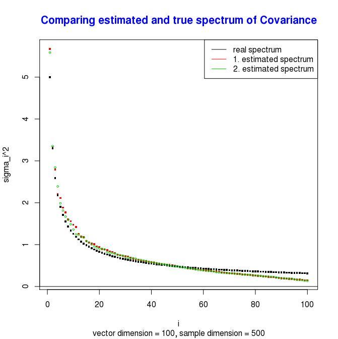
Figure 1:

The spectrum of the estimated covariance matrix seems to be almost like a “non-random function” of the spectrum of the original covariance matrix. One idea of recovering the true spectrum is the following. Take an arbitrary spectrum and simulate with this spectrum an estimated covariance matrix, then look at the spectrum and compare with the one we have at hand. Discard the original spectrum and then repeat this. However this seems very far from achieving any results at all. We will proceed a little more methodical.

1.4.2 The second stability phenomena, under the rescaling or reduction/blowup

Another phenomena, we observed in the data and our simulations is that the rescaled data’s sample covariance spectrum does not change too much in distribution. Let us explain, assume we take $n$ and $p$ to be a fixed proportion of a few times bigger such that their ratio remains the same. Then, we take the same distribution for the spectrum of the true covariance matrix for both simulations. In figure 2, we see the result of such simulations. There, the red line is the sample covariance spectrum when $n=200$ and $p=100$. The green line is the sample covariance with everything $100$ times bigger. That is, we take $n=20000$ and $p=10000$. The distribution of the true spectrum is taken the same for both simulations and is shown as the black line. For the green line we took only one in $100$ of the eigenvalues for the plot.

Hence, from Figure 2, we see that the distribution of the spectrum of the estimated covariance matrix is almost unchanged by blowing up everything by a factor $100$ whilst keeping the same distribution for the spectrum of the original covariance matrix. This tends to indicate that we do not need $n$ to be very large to get close to the limiting distribution. Indeed the free-probability theory, as we explain in Subsection 2.3, predicts that if we keep the same distribution for the spectrum of the original covariance matrix, then the spectrum of the estimated one converges as $n$ and $p$ go to infinity while we preserve their ratio. However, the interesting thing we noticed with real data, is that this phenomena of stability happens already with quite small data like here in Figure 2, and not just with dimension size in the billions.

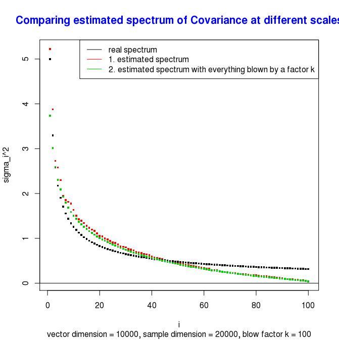
Figure 2:

Our spectrum reconstruction methods were first developed for when $Z$ has i.i.d rows with $0$ expectation which are multivariate normal. Our methods seems to work well even when the data is not exactly normal. Now let $\lambda_{1}>\lambda_{2}>\ldots>\lambda_{p}$ denote the eigenvalues of $E[Z^{t}Z]/n=COV[\vec{Z}]$, where again $\vec{Z}$ designates a random vector having same distribution then the rows of $Z$. Let $\widehat{\lambda}_{1}>\widehat{\lambda}_{2}>\ldots>\widehat{\lambda}_{p}$ designate the eigenvalues of the sample covariance matrix $Z^{t}Z/n$. The $i$-th estimation error is designated by $\Delta\lambda_{i}$ where $\Delta\lambda_{i}:=\widehat{\lambda}_{i}-\lambda_{i}$. In modern big data statistics one is more interested in the case where $n$ and $p$ both go to infinity at the same time, whilst their ratio $n/p$ converges to a constant. The case of traditional statistics is when $p$ is fixed and $n$ goes to infinity. In that case, there is an asymptotic formula for $\lambda_{i}$ which is totally different from our case. In the finite dimension case, one takes $\Delta\lambda$ to be asymptotically normal with expectation $0$ and a standard deviation of order $O\left(\frac{1}{\sqrt{n}}\right)$. It means that in this regime when $p$ is fixed and $n$ goes to infinity alone, the expectation of $\Delta\lambda$ is negligible compared to its standard deviation. In our case, the opposite holds, namely, the bias dominates the fluctuation so we can consider in a first approximation, $\Delta\lambda$ to be non-random. We develop an approximation formula for the eigenvectors and eigenvalues of the sample covariance. We do this via the formula for covariance error matrix [10], [9], [8] proven by Koltchinskii and Lounici, leading to the approximation formula (1.10) for the infinite dimensional case ($n$ and $p$ both going to infinity at the same time).

The second method is a fixed point method based on the eigenvectors of both the covariance and the sample covariance matrix.

1.4.3 Summary of the results

• Our first spectrum reconstruction method is based on the adaption of the finite dimensional asymptotic formula for Principal Components to the infinite dimensional case via the formula of Koltchinskii and Lounici [10] for the spectral norm of covariance estimation error matrix. The infinite dimensional approximation formula is given by:

  $$\Delta\lambda_{i}\approx\frac{\lambda_{i}}{n}\sum_{j\neq i}\frac{\widehat{\lambda}_{j}}{\widehat{\lambda}_{j}-\widehat{\lambda}_{i}},$$ (1.10)

  where $\Delta\lambda_{i}:=\widehat{\lambda}_{i}-\lambda_{i}$. Our first method, now consists in “solving” for $\lambda_{i}$ given all the sample covariance eigenvalues $\widehat{\lambda}_{j}$. Thus we obtain

  $$\lambda_{i}\approx\frac{\widehat{\lambda}_{i}}{1+\frac{1}{n}\sum_{j\neq i}\frac{\widehat{\lambda}_{j}}{\widehat{\lambda}_{j}-\widehat{\lambda}_{i}}}$$ (1.11)

  (For details on this method see subsection 2.1).

• Our second spectrum reconstruction method, consists of finding a fixed-point for the map

  $$\vec{\nu}\mapsto(\widehat{\lambda}_{1},\widehat{\lambda}_{2},\ldots,\widehat{\lambda}_{p})B(\vec{\nu}),$$

  where $\vec{\nu}=(\nu_{1},\nu_{2},\ldots,\nu_{p})$ with $\nu_{1}>\nu_{2}>\nu_{3}>\ldots>\nu_{p}\geq 0$ and $B(\vec{\nu})$ designating the matrix with the expected coefficients square of the unit eigenvectors of the original covariance matrix expressed in the basis of the unit eigenvectors of the sample covariance matrix. This matrix $B(\vec{\nu})$ is for when the spectrum of true covariance is equal to $\vec{\nu}$. (For details see Subsection 2.2).

1.4.4 Testing and consistency

We first tested our spectrum reconstruction methods on synthetic multivariate normal data, with a real spectrum taken from real life data and used simulations with this. This means, that we simulate multivariate normal data using as “more or less realistic” spectrum retrieved from real life data. That is a spectrum $s\mapsto\lambda_{s}$, which is convex and has more or less “the derivative going to $-\infty$ as $s$ approaches $0$”. Such kind of spectrum is what we noticed in real data. This is what you can see in Figure 3, where we have taken the spectrum from real stocks and estimated it, by just taking the spectrum for the sample covariance when sample size is much bigger than the vector size. In this way, we are pretty sure that the sample spectrum is close to the true underlying spectrum. This is so because when we hold $p$ fixed and let $n$ go to infinity, then the sample spectrum converges to the true spectrum.

For this synthetic data with realistic spectrum, the result of our reconstruction is surprisingly good as soon as $n/p\geq 2$ as can be seen in Figure 3.

Figure 3: Our reconstruction method for synthetic data

Below in Subsection 4.1, we test our methods and others on synthetic multivariate normal data and we see that except when the spectrum is close to being flat (close to being constant), our fixed-point-eigenvector method works really well. This only shows that when the data is truly hundred percent multivariate normal our methods work well with many examples of spectrae. However, real data is never exactly multivariate normal, only approximately. Thus we need to test our methods also on real data, and not just on synthetic data.

How can we be sure that it works with real data for recovering the “true underlying” covariance matrix’s spectrum, since we will never know that spectrum exactly? A first step, is to take a sample size much bigger than vector size (provided we have enough data for this). Then we see that increasing the sample size almost does not change the spectrum of the sample covariance matrix, we can assume that we have the true spectrum more or less. Indeed for $p$ fixed and $n$ going to infinity the sample spectrum always converges to the true spectrum, even if the model is not multivariate normal.

Thus, what we did is the following. We took two hundred stocks and their daily returns for $2000$ days. Then we took only $200$ days of real data (not synthetic data) and applied our spectrum recovery method (eigenvalue-fixed point method) to the real data with only 200 days. We compare the reconstructed spectrum to the sample covariance matrix spectrum with $2000$ days, where we assume that the sample spectrum with $2000$ days is close to the “true underlying” spectrum. The difference is quite small indicating that our method does work in the multivariate normal data and also on real life data. See for this Figure 4.

Figure 4: Our reconstruction methods with real data

In real life, the data is never exactly i.i.d. For example with stocks the true underlying covariance matrix will always change a little bit over time. Thus, even with the perfect reconstruction method, there must be a small discrepancy between the spectrum of the sample covariance matrix for $n$ large and the reconstructed spectrum. It is remarkable how little the difference between the two is in Figure 4!

Another, way to find out if our reconstruction methods work with real data, is to take a data set $Z$ of size $n$ times $p$. Then, we do the reconstructions for different restrictions of the sample size of our data set. That is we take $n_{1}<n$ and for the restricted data set where we take only $n_{1}$ samples instead of $n$, that is for

$$(\left(Z_{i,j}\right)_{i\in[1,n_{1}],j}$$

we do the reconstruction and compare it to the reconstruction using all $n$ samples. This is what can be seen in Figure 5. There we took $800$ stocks and once the $2000$ days and another time only $1000$ days. We took $50$ iterations of the fixed-point-eigenvector method. The first input for the fixed point method, was obtained by our asymptotic formula 1.10 for $\Delta\lambda$.

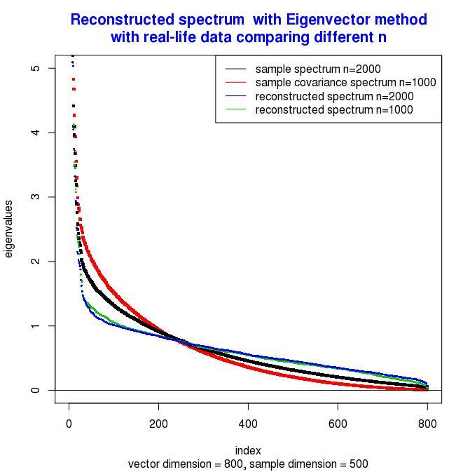
Figure 5: Reconstruction with real data but two different samples sizes compared

It is remarkable that though the spectrum of the sample covariance matrix is very different between the two cases $n=1000$ and $n=2000$, the reconstructed spectrum are pretty close to each other This is a strong indication that our reconstruction method works extremely well for real data. Indeed, it seems very unlikely that for very different inputs (the two sample covariance spectrae for $n=1000$ and the one for $n=2000$), would lead to almost same output. The only plausible explanation for why the outputs are about the same, is that they are close to the “true underlying spectrum”, which indeed is the same for both cases.

Note that to mitigate the fact that covariance matrix for stocks changes over time, we did not take the first $1000$ days, when we reduced the sample size. Instead, we chose $1000$ days at random.

1.5 Principal components

The eigenvalues of the covariance matrix $COV[\vec{Z}]$ are called Principal Components and we denote by $\vec{\mu}_{1},\vec{\mu}_{2},\ldots,\vec{\mu}_{p}$ the eigenvectors (principal components) of $COV[\vec{Z}]$, corresponding to the eigenvalues $\lambda_{1},\lambda_{2},\ldots,\lambda_{p}$. We assume that the eigenvalues are ordered as follows

$$\lambda_{1}>\lambda_{2}>\ldots>\lambda_{p}.$$

The quantities associated to the estimated covariance matrix are distinguished by a hat. Thus, the eigenvectors of the estimated covariance matrix $\widehat{COV}[\vec{Z}]$ are denoted by

$$\widehat{\vec{\mu}}_{1},\widehat{\vec{\mu}}_{2},\ldots,\widehat{\vec{\mu}}_{p},$$

with corresponding eigenvalues:

$$\widehat{\lambda}_{1},\hat{\lambda}_{2},\ldots,\widehat{\lambda}_{p}.$$

Why does one use eigenvectors? At least with some theoretical models the principal components with large eigenvalues correspond to factors. Let us see an example from finance which is related to our already mentioned Example 1.2. This model is not necessarily the one where principal components are most useful, but is in our opinion one of the best for pedagogical reasons.

One good example to understand where our $3$-order model for eigenvalues come from, are financial stocks. Assume that $\vec{Z}=({\color[rgb]{1,0,0}X},{\color[rgb]{1,0,0}Y},{\color[rgb]{0,1,0}Z},{\color[rgb]{0,1,0}W})$ denotes the daily change of value of four stocks.

• Stocks ${\color[rgb]{1,0,0}X}$ and ${\color[rgb]{1,0,0}Y}$ depend only on index ${\color[rgb]{1,0,0}T}$ and stocks ${\color[rgb]{0,1,0}Z}$ and ${\color[rgb]{0,1,0}W}$ depend only on index ${\color[rgb]{0,1,0}S}$. Thus,

  $${\color[rgb]{1,0,0}X}=a_{Z}{\color[rgb]{1,0,0}T}+0\cdot S+\epsilon_{X}$$

  $${\color[rgb]{1,0,0}Y}=a_{Y}{\color[rgb]{1,0,0}T}+0\cdot S+\epsilon_{Y}$$

  $${\color[rgb]{0,1,0}Z}=0\cdot T+b_{Z}{\color[rgb]{0,1,0}S}+\epsilon_{Z}$$

  $${\color[rgb]{0,1,0}W}=0\cdot T+b_{W}{\color[rgb]{0,1,0}S}+\epsilon_{W}$$

• We assume that ${\color[rgb]{0,1,0}S}$, ${\color[rgb]{1,0,0}T}$ and $\epsilon_{X},\epsilon_{Y},\epsilon_{Z},\epsilon_{W}$ are all independent of each other. The firm specific terms $\epsilon_{X},\epsilon_{Y},\epsilon_{Z},\epsilon_{W}$ are supposed to all have the same st. deviation $\sigma$. Furthermore $a_{Z},a_{Y},b_{Z},b_{W}$ are non-random and let $VAR[S]=VAR[T]=1$
  

With this finite sector model we get:

$$COV[\vec{Z}]=\left(\begin{array}[]{cccc}{\color[rgb]{1,0,0}a_{X}^{2}}&{\color[rgb]{1,0,0}a_{Z}a_{Y}}&0&0\\ {\color[rgb]{1,0,0}a_{Y}a_{Z}}&{\color[rgb]{1,0,0}a_{y}^{2}}&0&0\\ 0&0&{\color[rgb]{0,1,0}b_{Z}^{2}}&{\color[rgb]{0,1,0}b_{Z}b_{W}}\\ 0&0&{\color[rgb]{0,1,0}b_{W}b_{Z}}&{\color[rgb]{0,1,0}b_{w}^{2}}\end{array}\right)+\sigma^{2}I$$

where $I$ is identity matrix. The two eigenvectors with biggest eigenvalues are

$${\color[rgb]{1,0,0}\vec{\mu}_{1}=(a_{Z},a_{Y},0,0)}\;\;,\;\;{\color[rgb]{0,1,0}\vec{\mu}_{2}=(0,0,b_{Z},b_{W})}$$

with eigenvalues ${\color[rgb]{1,0,0}a_{Z}^{2}+a_{y}^{2}+\sigma^{2}}$, respectively ${\color[rgb]{0,1,0}b_{Z}^{2}+b_{W}^{2}+\sigma^{2}}$. We can easily extend this model to higher dimensional case. Assume for this that we have $2p$ stocks. The first $p$ are in the first sector and the second half in the second sector. Let

$$\vec{Z}=({\color[rgb]{1,0,0}Z_{1}},{\color[rgb]{1,0,0}Z_{2}},\ \ldots,{\color[rgb]{1,0,0}Z_{p}},{\color[rgb]{0,1,0}Z_{p+1}},{\color[rgb]{0,1,0}Z_{p+2}},\ldots,{\color[rgb]{0,1,0}Z_{2p}})$$

denote the daily change of value of our $2p$ stocks summarized in one vector. With this two sector model

$$Z_{i}=a_{i}{\color[rgb]{1,0,0}T}+\epsilon_{i}$$

for $i={\color[rgb]{1,0,0}1,\ldots,p}$ and

$$Z_{j}=b_{j}{\color[rgb]{0,1,0}S}+\epsilon_{j}$$

for $j={\color[rgb]{0,1,0}p+1,\ldots,2p}$ We assume ${\color[rgb]{0,1,0}S}$,${\color[rgb]{1,0,0}T}$ and $\epsilon_{i}$’s independent of each other with $0$ expectation. At first assume all $\epsilon_{i}$ have same standard deviation $\sigma$. We find then the following covariance matrix

$$COV[\vec{Z}]=\left(\begin{array}[]{ccccccc}{\color[rgb]{1,0,0}a_{1}^{2}}&{\color[rgb]{1,0,0}a_{1}a_{2}}&\ldots&{\color[rgb]{1,0,0}a_{1}a_{p}}&0&\ldots&0\\ {\color[rgb]{1,0,0}a_{2}a_{1}}&{\color[rgb]{1,0,0}a_{2}^{2}}&\ldots&{\color[rgb]{1,0,0}a_{2}a_{p}}&0&\ldots&0\\ &&&\ldots&&&\\ &&&\ldots&&&\\ {\color[rgb]{1,0,0}a_{p}a_{1}}&{\color[rgb]{1,0,0}a_{p}a_{2}}&\ldots&{\color[rgb]{1,0,0}a_{p}a_{p}}&0&\ldots&0\\ 0&0&\ldots&0&{\color[rgb]{0,1,0}b_{p+1}b_{p+1}}&\ldots&{\color[rgb]{0,1,0}b_{p+1}b_{2p}}\\ 0&0&\ldots&0&{\color[rgb]{0,1,0}b_{p+2}b_{p+1}}&\ldots&{\color[rgb]{0,1,0}b_{p+2}b_{2p}}\\ &&&\ldots&&&\\ &&&\ldots&&&\\ 0&0&\ldots&0&{\color[rgb]{0,1,0}b_{2p}b_{p+1}}&\ldots&{\color[rgb]{0,1,0}b_{2p}b_{2p}}\\ \end{array}\right)+\sigma^{2}I$$

With the model just introduced, the two eigenvectors with biggest eigenvalues are

$${\color[rgb]{1,0,0}\vec{\mu}_{1}=(a_{1},a_{2},\ldots,a_{p},0,\ldots,0)}\;\;,\;\;{\color[rgb]{0,1,0}\vec{\mu}_{2}=(0,\ldots,0,b_{p+1},b_{p+2},\ldots,b_{2p})}$$

with eigenvalues

$${\color[rgb]{1,0,0}a_{1}^{2}+a_{2}^{2}+\ldots+a_{p}^{2}+\sigma^{2}}=O(p),$$

respectively

$${\color[rgb]{0,1,0}b_{p+1}^{2}+b_{p+2}^{2}+\ldots+b_{2p}^{2}+\sigma^{2}}=O(p).$$

Other eigenvalue is $\sigma=O(1)$ with multiplicity $p-2$. Typically we take the data standardized (i.e. a correlation matrix) and the stocks have standard deviation $1$. This means that the coefficients $a_{i}$ and $b_{i}$ are correlation coefficients and are hence of order $O(1)$. In real life we have the sector factors (like here in the example $S$ and $T$) are not independent but depend all on the general economy. Hence, more realistically, we have a linear system of equation with factors, but the factors are not independent, then the vectors with the loadings of the factors

$${\color[rgb]{1,0,0}(a_{1},a_{2},\ldots,a_{p},0,\ldots,0)}\;\;,\;\;{\color[rgb]{0,1,0}(0,\ldots,0,b_{p+1},b_{p+2},\ldots,b_{2p})}$$

are no longer the principal components. However, we still have that the span of these two factor-vectors is the same as the span of the two first principal components $\vec{\mu}_{1}$ and $\vec{\mu}_{2}$. (At least if we assume that the $\epsilon_{j}$’s all have same variance and are independent of the factors $S$ and $T$ and of each other). Thus, in that case, the principal components are not interesting separately, but only in group. This means we are interested in their span.

If we can retrieve the span of the eigenvectors with large eigenvalues, we will use that span for dimension reduction and then look for the factors within that span. This is called rotation of factors which essentially tries to retrieve the factors from their span. Nevertheless, we see in our example that typically, the eigenvalues corresponding to factors are of order $O(p)$. The other eigenvalues coming from the terms $\epsilon_{i}$, are of order $O(1)$. Thus, if we were given the “true” spectrum $\lambda_{1},\lambda_{2},\ldots,\lambda_{p}$, we would try to see where the big eigenvalues “end”, and where the smaller eigenvalues “start” in the spectrum. In reality this is often very difficult to see from the estimated spectrum $\widehat{\lambda}_{1},\widehat{\lambda}_{2},\ldots,\widehat{\lambda}_{p}$ where the “big eigenvalues stop” and where the “small eigenvalues start”. This is so because if $n$ is not much larger than $p$ there is a big estimation error in the spectrum of the covariance matrix. This is to say that there can be a big difference between

$$\lambda_{1},\lambda_{2},\ldots,\lambda_{p},$$ (1.12)

and

$$\widehat{\lambda}_{1},\widehat{\lambda}_{2},\ldots,\widehat{\lambda}_{p},$$ (1.13)

when $n$ is not much bigger than $p$. (In our practical experience we need $n$ to be about $10$ times bigger than $p$ in order to be able to consider that the estimated spectrum 1.13 can be considered identical to the true spectrum 1.12 in practice). Therefore the usual error when taking the estimated spectrum 1.13 instead of the true spectrum 1.12 is a sort of smoothing. (We will describe below why) Due to this, very often, in the original spectrum we can really see where the “large eigenvalues end in the true spectrum” which often is no longer easily visible in the estimated spectrum 1.13 due to the smoothing. Indeed, the passage corresponds to an “elbow” in the original spectrum 1.12 which is no longer visible in the estimated spectrum 1.13.

That is one should be able to better identify where the eigenvalues corresponding to factors end and where in the spectrum, the noise starts. Another motivation, is that with normal data, if we are given the original spectrum 1.12, we can simulate everything. This can then allow as we explain below to see if the estimated eigenvectors are typically very different from the true ones.

2 Our recovering methods and the free probability approach explained

We explain next our two algorithms and where they come from. Given as input the spectrum of $\widehat{COV}[\vec{X}]$

$$\widehat{\lambda}_{1},\widehat{\lambda}_{2},\ldots,\widehat{\lambda}_{p}$$

we try to recover the spectrum of the original covariance matrix $COV[\vec{X}]$

$$\lambda_{1},\lambda_{2},\ldots,\lambda_{p}.$$

In the last subsection of this section we explain the general idea behind the free probability approach.

Let us summarize the different methods.

• Free probability based approach. This approach has first been pioneered by EI Karoui [5], was further developed by Silverstein [18], Bai and Yin [1], Yin, Bai and Krishnaiah [22] and recently Ledoit and Wolf [12], [16] and [13].

• Moment methods. [11]. This is the same methods as is usually for proving the semi-circular law. But, then for the higher moments, too much computation is needed, but we definitely would use moments which are not too high, when dealing with big real life data as a double insurance.

• Modeling “true” spectrum with low dimension parameter function family and then apply asymptotic statistics.

• Shrinkage method which was pioneered by Stein [19], see also Bickel and Levina [3] or Donoho [7].

• Our methods.

  1. Finite dimensional asymptotic formula adapted to the infinite dimensional case using the formula of Koltchinskii and Lounici [10] for covariance error matrix spectral norm.

  2. Fixed point of map defined with the matrix of second moments of principal component eigenvectors. For this we take the eigenvectors of the true covariance matrix expressed in the basis of the sample covariance eigenvectors as a function of a given spectrum $\vec{\nu}=(\nu_{1},\nu_{2},\ldots,\nu_{p})$.

Let us next present our two methods more in detail:

2.1 Our first method based on asymptotic finite dimensional formula adapted via Koltchinski and Lounici

This method with real non-sparse data works quite well as long as $p/n$ is not much bigger than $1$. It is a simple formula, which gives an approximation to the correcting term to obtain the values $\lambda_{i}$ from the eigenvalues $\widehat{\lambda}_{i}$, $i=1,2,\ldots,p$ of the estimated covariance matrix. The formula for approximating the $i$-th error between the eigenvalue of the covariance matrix, and the corresponding eigenvalue of the estimated covariance matrix is given. This error is $\Delta\lambda_{i}:=\widehat{\lambda}_{i}-\lambda_{i}$ can be approximated as in 1.10. One can then “solve” the approximation (1.10) for $\lambda_{i}$ to obtain the approximation for the true eigenvalue $\lambda_{i}$ given in (1.11). But, where does the formula (1.10) come from in the first place? In an upcoming paper, we will present exact calculations, which are rather elaborated. Here we can already show the main idea and how the result of Koltschinskii and Lounici [10] is essential in getting the formula. We start with a three dimensional example:

Assume we have a three dimensional random vector with independent normal entries $\vec{X}=(X,Y,Z)$ having each expectation $0$. We assume that the standard deviations are decreasing: $\sigma_{X}>\sigma_{Y}>\sigma_{Z}$. The covariance matrix we consider is:

$$COV[\vec{X}]=\left(\begin{array}[]{ccc}\sigma_{X}^{2}&0&0\\ 0&\sigma_{Y}^{2}&0\\ 0&0&\sigma_{Z}^{2}\end{array}\right).$$ (2.1)

Now, for that covariance matrix, the eigenvectors are the three canonical vectors: $(1,0,0)$, $(0,1,0)$ resp. $(0,0,1)$ with eigenvalues $\sigma_{X}^{2}$, $\sigma_{Y}^{2}$ and $\sigma_{Z}^{2}$. We are going to look at what happens to the eigenvectors, when instead of the covariance matrix we take the estimated covariance matrix. Let us explain more in detail the setting.

Let us assume that $\vec{X},\vec{X}_{1},\vec{X}_{2},\ldots$ are independent copies of the vector $\vec{X}$, where $\vec{X}_{i}=(X_{i},Y_{i},Z_{i})$. We assume that we have $n$ such vectors and want to estimated the covariance matrix (2.1). Let $X$ be the $n\times 3$ matrix, where the $i$the row of $X$ is equal to $\vec{X}_{i}$. The estimated covariance matrix is then given by

$$\widehat{COV}[\vec{X}]:=\frac{X^{t}\cdot X}{n}$$

The difference between true and estimated covariance matrix is denoted by $E$ so that

$$E=COV[\vec{X}]-\frac{X^{t}\cdot X}{n}.$$

Instead of the true covariance matrix $COV[\vec{X}]$ we consider the perturbated matrix

$$\widehat{COV}[\vec{X}]=COV[\vec{X}]+E$$

which is obtained from the true covariance matrix by adding $E$.

There is a general equation for what happens with eigenvectors when we add a perturbation $E$ to a matrix $A$. Say that $\vec{\mu}$ is an unitary eigenvector of $A$ with eignevalue $\lambda$. Let $\alpha\vec{\mu}+\Delta\vec{\mu}$ be a unitary eigenvector of $A+E$ with eigenvalue $\lambda+\Delta\lambda$. Then, we have

$$A\vec{\mu}=\lambda\vec{\mu}$$ (2.2)

and also

$$(A+E)(\alpha\vec{\mu}+\Delta\vec{\mu})=(\lambda+\Delta\lambda)(\alpha\vec{\mu}+\Delta\vec{\mu}).$$ (2.3)

Subtracting $\alpha$ times (2.2) from (2.3) we find

$$(A-(\lambda+\Delta\lambda)I+E)\Delta\vec{\mu}=-\alpha E\cdot\vec{\mu}+\alpha\Delta\lambda\cdot\vec{\mu}$$ (2.4)

Now we can rewrite equation (2.4) with $A$ being the covariance matrix 2.1. We consider the eigenvector $\vec{\mu}=(1,0,0)$ of $A$ with eigenvalue $\lambda=\sigma_{X}^{2}$. We take $\Delta\mu$ perpendicuar to $\vec{\mu}$. In the present, case this means that $\Delta\mu=(0,\Delta\mu_{Y},\Delta\mu_{Z})$. Thus, without leaving out terms, we find the following exact equation:

$$\left(\begin{array}[]{ccc}0&0&0\\ 0&\sigma_{Y}^{2}-\sigma_{X}^{2}-\Delta\lambda&0\\ 0&0&\sigma_{Z}^{2}-\sigma_{X}^{2}-\Delta\lambda\end{array}\right)\left(\begin{array}[]{c}0\\ \Delta\mu_{Y}\\ \Delta\mu_{Z}\end{array}\right)=$$

$$=-\alpha\left(\begin{array}[]{c}E_{11}\\ E_{21}\\ E_{31}\end{array}\right)+\alpha\left(\begin{array}[]{c}\Delta\lambda\\ 0\\ 0\\ \end{array}\right)-\left(\begin{array}[]{ccc}0&0&0\\ 0&E_{22}&E_{23}\\ 0&E_{32}&E_{33}\end{array}\right)\left(\begin{array}[]{c}0\\ \Delta\mu_{Y}\\ \Delta\mu_{Z}\end{array}\right)-\left(\begin{array}[]{ccc}0&E_{12}&E_{13}\\ 0&0&0\\ 0&0&0\end{array}\right)\left(\begin{array}[]{c}0\\ \Delta\mu_{Y}\\ \Delta\mu_{Z}\end{array}\right)$$

the above equation for matrices can be “separated into two parts”. First the single equation for $\Delta\lambda$:

$$\Delta\lambda=E_{11}+\frac{1}{\alpha}(E_{12}\Delta\mu_{Y}+E_{13}\Delta\mu_{Z}).$$ (2.5)

Then the $p-1$ dimensional equation for $\Delta\vec{\mu}$ given as follows:

$$\left(\left(\begin{array}[]{cc}\sigma_{Y}^{2}-\sigma_{X}^{2}-\Delta\lambda&0\\ 0&\sigma_{Z}^{2}-\sigma_{X}^{2}-\Delta\lambda\end{array}\right)+\left(\begin{array}[]{cc}E_{22}&E_{23}\\ E_{32}&E_{33}\end{array}\right)\right)\left(\begin{array}[]{c}\Delta\mu_{Y}\\ \Delta\mu_{Z}\end{array}\right)=$$

$$=-\alpha\left(\begin{array}[]{c}E_{21}\\ E_{31}\end{array}\right)$$

If $\Delta\lambda$ is given we can solve the above equation for $\Delta\vec{\mu}=(\Delta\mu_{Y},\Delta\mu_{Z})$. We find

$$\left(\begin{array}[]{c}\Delta\mu_{Y}\\ \Delta\mu_{X}\end{array}\right)=-\alpha\cdot(I+D_{1}\cdot E_{1})^{-1}\cdot D_{1}\vec{E}_{1}=-\alpha(D_{1}^{-1}+E_{1})^{-1}\vec{E}_{1},$$

where

$$D_{1}=\left(\begin{array}[]{cc}\sigma_{Y}^{2}-\sigma_{X}^{2}-\Delta\lambda&0\\ 0&\sigma_{Z}^{2}-\sigma_{X}^{2}-\Delta\lambda\end{array}\right)^{-1}$$

and $E_{1}$ is the reduce matrix obtained from $E$ by deleting the first row and first column:

$$E_{1}=\left(\begin{array}[]{cc}E_{22}&E_{23}\\ E_{32}&E_{33}\end{array}\right).$$

Also, $\vec{E}_{1}$ is the first column of the matrix $E$ where we delete the first entry.

$$\vec{E}_{1}=\left(\begin{array}[]{c}E_{21}\\ E_{31}\end{array}\right).$$

Now, in general with a higher dimensional situation and say you want to estimate the $i$-th eigenvector. You get the same type formula:

$$\Delta\vec{\mu}_{i}=-\alpha(I+D_{i}\cdot E_{i})^{-1}\cdot D_{i}\vec{E}_{i},$$ (2.6)

where $E_{i}$ is the reduced matrix obtained from $E$ by deleting the $i$ row and column. Furthermore, $D_{i}$ is the diagonal $p\times p$-matrix, obtained by deleting the $i$-th row and column from the diagonal matrix having as $j$ entry in the diagonal $1/(\sigma_{j}^{2}-\sigma_{i}^{2}-\delta\lambda_{i})$. Again $\vec{E}_{i}$ is the vector obtained from taking the $i$-th column of $E$ and deleting the $i$-th entry. Now, we assume that the spectral norm of $D_{i}E_{i}$ is much less than one, so that

$${\tt assumption:}\;\;|D_{i}E_{i}|<<1$$

In that case, we can leave out in formula 2.6 the matrix $D_{i}E_{i}$ to obtain the approximation

$$\Delta\vec{\mu}_{i}\approx-\alpha D_{i}\vec{E}_{i}.$$

We plug the last approximation back into 2.5 to obtain:

$$\Delta\lambda\approx-\left(\frac{E_{12}^{2}}{\sigma^{2}_{Y}-\sigma^{2}_{X}-\Delta\lambda}+\frac{E_{13}^{2}}{\sigma^{2}_{Z}-\sigma^{2}_{X}-\Delta\lambda}\right),$$ (2.7)

where we also left out $E_{11}$ since it is a smaller term of order $O(\frac{\sigma_{X}^{2}}{\sqrt{n}})$. Let

$$N_{12}=\frac{E_{12}}{\sigma_{X}\sigma_{Y}}\cdot\sqrt{n},N_{13}=\frac{E_{13}}{\sigma_{X}\sigma_{z}}\cdot\sqrt{n}.$$

By central limit theorem, $N_{12}$ and $N_{13}$ are close to standard normal. On top of it they are uncorrelated. Hence, we can write equation 2.7 as

$$\Delta\lambda\approx-\frac{\sigma_{X}^{2}}{n}\left[(\frac{N_{12}^{2}\sigma_{Y}^{2}}{\sigma^{2}_{Y}-\sigma^{2}_{X}-\Delta\lambda}+\frac{N_{13}^{2}\sigma_{Z}^{2}}{\sigma^{2}_{Z}-\sigma^{2}_{X}-\Delta\lambda}\right],$$

In the real data sets we have in mind, typically $\Delta\lambda$’s standard deviation is of smaller order than $\Delta\lambda$. This allows to take the expectation on the right side of the last approximation above to find:

$$\Delta\lambda\approx-\frac{\sigma_{X}^{2}}{n}\left[\frac{\sigma_{Y}^{2}}{\sigma^{2}_{Y}-\sigma^{2}_{X}-\Delta\lambda}+\frac{\sigma_{Z}^{2}}{\sigma^{2}_{Z}-\sigma^{2}_{X}-\Delta\lambda}\right],$$

where we acted as if $\Delta\lambda$ would be a constant and we used the fact that $E[N_{12}^{2}]=E[N_{13}^{2}]=1$. The values $\sigma_{Y}^{2}$ and $\sigma_{Z}^{2}$ are not known, so we replace them by their estimates leading to our formula:

$$\Delta\lambda\approx-\frac{\sigma_{X}^{2}}{n}\left[\frac{\widehat{\sigma}_{Y}^{2}}{\widehat{\sigma}^{2}_{Y}-\widehat{\sigma}^{2}_{X}}+\frac{\widehat{\sigma}_{Z}^{2}}{\widehat{\sigma}^{2}_{Z}-\widehat{\sigma}^{2}_{X}}\right],$$ (2.8)

where we also used that $\widehat{\sigma}_{X}^{2}=\sigma_{X}^{2}+\Delta\lambda$.

With a bigger normal random vector

$$\vec{X}=(X_{1},X_{2},\ldots,X_{p})$$

with independent normal entries with $0$ expectation and

$$\lambda_{i}=VAR[X_{i}]=\sigma_{i}^{2}$$

for all $i=1,2,\ldots,p$ we can generate a $p$-dimensional random vector and then we can derive similarly to (2.8) as in the three dimensional case

$$\Delta\lambda_{i}:=\widehat{\lambda}_{i}-\lambda_{i}=\widehat{\sigma}_{i}^{2}-\sigma_{i}^{2}\approx-\frac{\sigma_{i}^{2}}{n}\sum_{j\neq i}\frac{\widehat{\sigma}_{j}^{2}}{\widehat{\sigma}_{j}^{2}-\widehat{\sigma}_{i}^{2}}.$$ (2.9)

But this is just our approximation formula given in (1.10). The fact that we took a normal vector with independent entries is not a restriction. When we take as basis the principal component of the covariance matrix, the components become independent, so that formula (2.9) holds not just for normal with independent entries but also for normal vector with entries not independent of each other.

The only problem for proving this formula in $p$-dimensional case, is bounding the spectral norm of the matrix product $D_{i}E_{i}$. For this we note that this spectral norm is equal to the spectral norm of

$$|D_{i}|^{1/2}E_{i}|D_{i}|^{1/2}$$ (2.10)

where $|D_{i}|^{1/2}$ represents the diagonal matrix obtained from $D_{i}$ by replacing each diagonal entry by the square root of the absolute value for the corresponding entry. The matrix given in (2.10) can be viewed as a error-sample covariance matrix, but when the “true” spectrum is modified. The modification consists of taking $\sigma^{2}_{j}/(\sigma^{2}_{j}-\sigma_{j}^{2})$ instead of $\sigma_{j}^{2}$ for all $j$ eigenvalue of a true covariance matrix, for all $j\neq i$. We can bound the spectral norm of (2.10) with the result of Koltchinskii and Lounici [10] for covariance error matrix spectral norm. This is why the result of Koltchinskii and Lounici is so important to us. As we already mentioned, the detail of these calculations will be explained more in detail in an upcoming paper, however the main idea is just explained above.

2.2 Our second method: fixed-point for eigenvector-entry-square map

Take a vector of non-random coefficients

$$\vec{a}=(a_{1},a_{2},\ldots,a_{p}).$$

Consider the scalar product

$$\vec{a}\cdot\vec{Z}=a_{1}Z_{2}+\ldots+a_{p}Z_{p}.$$ (2.11)

The scalar product (2.11) has expectation $0$. To estimate its variance since the expectation is $0$, we can take the average of independent copies square

$$\widehat{VAR}[\vec{a}\cdot\vec{Z}]:=\widehat{E}[\left(\vec{a}\cdot\vec{Z}\right)^{2}]=\frac{(\vec{a}\cdot\vec{Z}_{1})^{2}+\ldots+(\vec{a}\cdot\vec{Z}_{n})^{2}}{n}=\vec{a}^{t}\frac{Z^{t}Z}{n}\vec{a},$$ (2.12)

where $\vec{Z}_{i}$ denotes the $i$-th row of the $n\times p$-matrix $Z$. Recall that the $\vec{Z}_{1},\vec{Z}_{2},\ldots$ is an i.i.d. sequence of independent copies of $\vec{Z}$. Thus our estimate is a mean of $n$ nicely behaved ( exponential decaying tail) independent variables. Hence, the estimation error of (2.12) is with high probability of order $O(\frac{1}{\sqrt{n}})$. This is to say that

$$\frac{(\vec{a}\cdot\vec{Z}_{1})^{2}+\ldots+(\vec{a}\cdot\vec{Z}_{n})^{2}}{n}=E[(\vec{a}\cdot\vec{Z}_{1})^{2}]+O\left(\frac{\sigma_{j}^{2}}{\sqrt{n}}\right).$$ (2.13)

Now, take $\vec{Z}$ to be a row verctor and $\vec{a}$ to be a column vector. Then

$$E[(\vec{a}\cdot\vec{Z})^{2}]=E[\vec{a}^{t}\vec{Z}^{t}\vec{Z}\vec{a}]=\vec{a}^{t}E[\vec{Z}^{t}\vec{Z}]\vec{a}=\vec{a}^{t}COV[\vec{Z}]\vec{a}$$ (2.14)

and so if $\vec{a}$ is the $j$-th unit-eigenvector of the original covariance matrix, with eigenvalue $\lambda_{j}$, then the expression on the right most side of equation 2.14 is equal to

$$\vec{a}^{t}COV[\vec{Z}]\vec{a}=\lambda_{j}.$$ (2.15)

In that case combining this with (2.14), yields

$$E[(\vec{a}\cdot\vec{Z})^{2}]=\lambda_{j}$$

and hence combining this with 2.12 and 2.13

$$\vec{a}^{t}\frac{Z^{t}Z}{n}\vec{a}=\lambda_{j}+O\left(\frac{\sigma_{j}^{2}}{\sqrt{n}}\right).$$ (2.16)

The last equation above tells us that if we would know the $j$-th unit eigenvector of the original covariance matrix $COV[\vec{Z}]$, then we would be able to reconstruct the $j$-th eigenvalue $\lambda_{j}$ up to a smaller order term. Now let $U$ be the unitary matrix whose columns are the unitary eigenvectors of the matrix $\frac{Z^{t}Z}{n}$ in the order of decreasing eigenvalues. Then, we can rewrite (2.16) as follows

$$\lambda_{j}=\vec{a}^{t}U(U^{t}\frac{Z^{t}Z}{n}U)U^{t}\vec{a}+O\left(\frac{\sigma^{2}_{j}}{\sqrt{n}}\right).$$

Now, $U^{t}\frac{Z^{t}Z}{n}U$ is the diagonal matrix of estimated eigenvalues $\widehat{\lambda}_{j}$. (Recall that $\widehat{\lambda}_{j}$ designated the $j$-th eigenvalue of the estimated covariance matrix $\widehat{COV}(\vec{Z})=\frac{Z^{t}Z}{n}$.) Furthermore $U^{t}\vec{a}$ is the $j$-th eigenvector of the true covariance matrix $COV[\vec{Z}]$ espressed in the basis of the eigenvectors of $\frac{Z^{t}Z}{n}$. So we have

$$\lambda_{j}=\vec{a}^{t}U\left(\begin{array}[]{cccccc}\widehat{\lambda}_{1}&0&0&\ldots&0\\ 0&\widehat{\lambda}_{2}&0&\ldots&0\\ 0&0&\widehat{\lambda}_{3}&\ldots&0\\ \ldots\\ 0&0&0&\ldots&\widehat{\lambda}_{p}\end{array}\right)U^{t}\vec{a}+O\left(\frac{\sigma^{2}_{j}}{\sqrt{n}}\right).$$ (2.17)

Consequently, the estimated eigenvalues $\widehat{\lambda}_{j}$ have a fluctuation of smaller order than their own values and thus it makes sense to assume that

$$O(\sigma_{\widehat{\lambda}_{j}})<<O(E[{\widehat{\lambda}_{j}}]).$$

What this means is that we can replace in (2.17) the $\widehat{\lambda}_{i}$’s by their expectation. This gives an error of smaller order. Hence we find that

$$\lambda_{j}=\vec{a}^{t}U\left(\begin{array}[]{cccccc}E[\widehat{\lambda}_{1}]&0&0&\ldots&0\\ 0&E[\widehat{\lambda}_{2}]&0&\ldots&0\\ 0&0&E[\widehat{\lambda}_{3}]&\ldots&0\\ \ldots\\ 0&0&0&\ldots&E[\widehat{\lambda}_{p}]\end{array}\right)U^{t}\vec{a}+O\left(\frac{\sigma^{2}_{j}}{\sqrt{n}}\right).$$ (2.18)

But now in the expression on the right side of the approximation above only $U^{t}\vec{a}$ is random. What we can do now is to take the coefficients of $U^{t}\vec{a}$ from another simulation and we would still have the same approximation error size. We will simulate the eigenvectors of another matrix and write them in the basis of the eigenvectors of the estimated covariance matrix.

More precisely, say that for another simulation $\vec{b}_{j}$ is the vector expressing the $j$-th unitary eigenvector of the original covariance matrix $COV[\vec{Z}]$ expressed in the unitray basis of eigenvectors of the estimated covariance matrix. Let $b_{ij}$ be the $i$-th entry of the vector $\vec{b}_{j}$. Taking the expectation of (2.18) yields

$$\lambda_{j}=E\left[\vec{b}_{j}^{t}\left(\begin{array}[]{cccccc}E[\widehat{\lambda}_{1}]&0&0&\ldots&0\\ 0&E[\widehat{\lambda}_{2}]&0&\ldots&0\\ 0&0&\widehat{\lambda}_{3}&\ldots&0\\ \ldots\\ 0&0&0&\ldots&E[\widehat{\lambda}_{p}]\end{array}\right)\vec{b}_{j}\right]+O\left(\frac{\sigma^{2}_{j}}{\sqrt{n}}\right)=\sum_{i=1}^{p}E[b_{ij}^{2}]E[\widehat{\lambda}_{i}]+O\left(\frac{\sigma^{2}_{j}}{\sqrt{n}}\right)$$ (2.19)

where the last approximation above is up to a smaller order term. Now, note that the coefficients $\widehat{\lambda}_{i}$ are known to us, and since they are very close to their expectation we assume that $E[\widehat{\lambda}_{i}]$ is known.

Now let $B$ be the matrix which has as $(i,j)$-entry the expectation of the square coefficient $b^{2}_{ij}$. This means that $B$ is the matrix who’s $j$-column represents the expected coefficient square of the representation of the $j$-th unitary eigenvector of the true covariance matrix $COV[\vec{Z}]$ in the unitary basis of the eigenvectors for the sample covariance matrix. Hence

$$B_{ij}=E[b_{ij}^{2}].$$ (2.20)

Of course the matrix $B$ depends on the chosen spectrum $\vec{\lambda}$,

$$\vec{\lambda}=(\lambda_{1},\lambda_{2},\ldots,\lambda_{p})$$

we took to simulate the matrix $B$.

Hence we write

$$B=B(\vec{\lambda}).$$

Recall our usual convention that $\lambda_{1}>\lambda_{2}>\ldots>\lambda_{p}$.

Thus, (2.19) is an equation for every $j\in\{1,2,\ldots,p\}$. We can write these $j$ equations in matrix/vector form as

$$\vec{\lambda}=(E[\widehat{\lambda}_{1}],\ldots,E[\widehat{\lambda}_{p}])\cdot B(\vec{\lambda})+\vec{\epsilon}(\vec{\lambda}),$$ (2.21)

where $\vec{\epsilon}(\vec{\lambda})$ is a smaller order term, which is to be considered a non-random function of the vector $\vec{\lambda}$. The right side of the above equation (2.21) can be viewed as a non-random function of the imput $\vec{\lambda}$. The key is that we can interpret (2.21) as saying that the true spectrum $\vec{\lambda}$ is a fixed point for that map given in (2.21). However, the term $\vec{\epsilon}(\vec{\lambda}$ is a smaller order term and not observable which we are going to neglect.

Our reconstruction algorithm for the true spectrum $\vec{\lambda}$ consists of finding a fixed point for the map

$$\vec{\nu}\mapsto(E[\widehat{\lambda}_{1}],\ldots,E[\widehat{\lambda}_{p}])\cdot B(\vec{\nu})$$ (2.22)

where $\vec{\nu}=(\nu_{1},\nu_{2},\ldots,\nu_{p})$ with $\nu_{1}>\nu_{2}>\ldots>\nu_{p}\geq 0$.

Here, again $B(\vec{\nu})$ consists of the $p\times p$ matrix who’s $ij$ entry is the expectation of the square of the coefficient of the $j$-th eigenvector of the original covariance matrix written in the basis of the sample covariance matrix given that the true spectrum is $\vec{\nu}$. In other words, given $\vec{\nu}$, we simulate the data many times using $\vec{\nu}$ as the true spectrum of the $COV[\vec{Z}]$. For every simulation we compute the matrix representing the unitary eigenvectors of the original matrix expressed in the basis of the unitary eigenvectors of the simulated sample covariance matrix. Then, we take the average of these coefficients square, over the different simulations. This gives us a good approximation of $B(\vec{\nu})$.

Now the key part is that we start with any spectrum $\lambda_{0}$ and iterate the map. Otherwise stated we construct a sequence of spectrae

$$\vec{\nu}_{0},\vec{\nu}_{1},\ldots.$$ (2.23)

Each of the $\vec{\nu}_{k}$ is a positive $p$ dimensional vector such that

$$\vec{\nu}_{1}=(E[\widehat{\lambda}_{1}],\ldots,E[\widehat{\lambda}_{p}])B(\vec{\nu}_{0})$$

and in general

$$\vec{\nu}_{k+1}=(E[\widehat{\lambda}_{1}],\ldots,E[\widehat{\lambda}_{p}])B(\vec{\nu}_{k})$$

If the sequence (2.23) converges, then it must converge to a fixed point. And since $\vec{\lambda}$ is a fixed point, we assume that

$$\vec{\lambda}\approx\lim_{k\rightarrow\infty}\vec{\nu}_{k}$$

up to smaller order error term.

2.3 Free probability approach

Assume $A$ and $B$ are two $n\times n$ symmetric random matrices which we take to be independent of each other.

Let $\mu$ and $\nu$ be two distributions on the real line. We choose the eigenvalues of $A$, such that the distribution of the eigenvalues converge to a random variable distributed according to $\mu$. Similarly assume that the eigenvalues of $B$ distribute in the limit according to $\nu$. In addition, assume that the distribution of the matrices are invariant under conjugation by unitary matrices. We can construct such matrices as follows, we chose the direction of all the eigenvectors of $A$ and $B$ at random so that these directions are equiprobably pointing into any direction in space. For example take standard normal symmetric matrices and use the eigendecomposition into the spectral part and the eigenvectors part. The matrix $U$ formed by the eigenvectors is a unitaty matrix and we can form the matrix

$$A=UDU^{\prime}$$

where the matrix $D$ is a diagonal matrix with the diagonal being the eigenvalues of $A$ which distribute in the limit according to $\mu$. We do the same thing for $B$ and in addition we assume the choices independent of the choices of $A$. Thus we produced here $A$ and $B$ which are now independent of each other if we choose the eigenvalues and the eigenvectors independent of each other.

Consider now the matrix product $AB$. Free probability theory demonstrates that as the dimension of the matrices tends to infinity, the empirical distribution of the spectrum of $AB$ converges in distribution [20, 21] to the so called free multiplicative convolution of $\mu$ and $\nu$ and is denoted by $\mu\boxtimes\nu$. The best way to understand this is via the so called $S$ transform introduced by Voiculescu and described in [21]. This is very similar in spirit with the Fourier transform from the classical probability. For any distribution $\mu$, it assigns a formal power series $S_{\mu}(z)$ which can be also understood as a complex analytic function in some region. The main property of this transform is that

$$S_{\mu\boxtimes\nu}(z)=S_{\mu}(z)S_{\nu}(z).$$

Coming back to our problem, notice that $\vec{X}=(X_{1},X_{2},\ldots,X_{p})$ is a normal vector with independent entries. Define now $\sigma^{2}_{j}:=VAR[X_{j}]=\lambda_{j}$. We can write $\vec{X}$ as a diagonal matrix times a vector with standard normal entries as follows

$$\vec{X}=\vec{N}\Sigma$$

where we define $\Sigma$ as the diagonal matrix with diagonal vector given by $\sigma_{1},\sigma_{2},\dots,\sigma_{p}$.

Now, all the rows of the matrix $X$ are i.i.d. and each is distributed like the vector $\vec{X}$. Therefore we can write the matrix $X$ as

$$X=N\cdot\Sigma$$

where $N$ is a $n$ time $p$ matrix with all entries independent standard normal. This in turn gives the estimated covariance matrix as

$$\widehat{COV}[X]=\Sigma\cdot\frac{N^{t}\cdot N}{n}\cdot\Sigma.$$

Since for any square matrices $C$ and $D$, the spectrum of $C\cdot D$ is equal to the spectrum of $D\cdot C$ we conclude that the spectrum of $\widehat{COV}[X]$ is equal to the spectrum of

$$\frac{1}{n}N^{t}\cdot N\cdot\Sigma^{2}$$ (2.24)

If $p$ is large enough and $p/n$ stays approximately $r$, then the empirical distribution of (2.24) is approximately the free product of the spectrum of $\Sigma^{2}$ and the matrix:

$$\frac{1}{n}N^{t}\cdot N.$$ (2.25)

The matrix 2.25 is known to converge to Marchenko-Pastur distribution given by

$$\alpha(dx)=\frac{\sqrt{(\rho_{+}-x)(x-\rho_{-})}}{2\pi\rho x}1_{[\rho_{-},\rho_{+}]}dx$$

where $\rho_{\pm}=(1\pm\sqrt{r})^{2}$ and $n$ and $p$ both go to infinity while $p/n$ is an approximately fixed proportion of $\rho$ which we take to be between $(0,1)$.

In the limit, the distribution of eigenvalues of $\widehat{COV}(X)$ becomes

$$\widehat{\mu}=\mu\boxtimes\alpha$$

where $\mu$ is the limiting distribution of the spectrum of $\Sigma$. Thus, if we use the $S$ transform we get now

$$S_{\widehat{\mu}}(z)=S_{\mu}(z)S_{\alpha}(z).$$

Recall that the $S$ transform is given by

$$S_{\mu}(z)=\frac{z+1}{z}m_{\mu}^{-1}(z)$$ (2.26)

where the inverse is the formal power series inverse and we assume that $\int x\mu(dx)\neq 0$ with

$$m_{\mu}(z)=\sum_{m\geq 1}\left(\int x^{n}\mu(dx)\right)z^{n}.$$

Notice here that the inverse in (2.26) can also be made analytically by restricting the domain of $z$ to a proper domain in the complex plane.

From this we can invert the relation into

$$S_{\mu}(z)=\frac{S_{\widehat{\mu}}(z)}{S_{\alpha}(z)}$$

and thus

$$\mu=S^{-1}\left(\frac{S_{\widehat{\mu}}(z)}{S_{\alpha}(z)}\right)$$ (2.27)

which is a way of recovering the distribution of the eigenvalues of $\Sigma$ in the limit.

Now, recall what our fundamental problem is. Given the spectrum of the estimated covariance matrix $\widehat{COV}[\vec{X}]$ reconstruct the spectrum of the original covariance matrix $COV[\vec{X}]$, which is given by

$$\sigma^{2}_{1}>\sigma^{2}_{2}>\ldots>\sigma^{2}_{p}.$$

If we consider that the estimated covariance matrix spectrum is very close in distribution to the free product of the Marchenko-Pastur and $\Sigma^{2}$ (because the dimension is big enough), then we can conclude that reconstructing the spectrum $\Sigma$ can be done using an approximation to (2.27). Thus we have the following approximation

$$S_{\widehat{COV}[\vec{X}]}(z)=S_{\frac{N\cdot N}{n}\cdot\Sigma^{2}}(z)\approx S_{\frac{N\cdot N}{n}}(z)\cdot S_{\Sigma^{2}}(z)$$

which then leads to

$$\Sigma^{2}\approx S^{-1}\left(\frac{S_{\widehat{COV}[\vec{X}]}}{S_{\frac{N\cdot N}{n}}}\right).$$

This is a nice description in terms of free probability. On the other hand we still do not have a very good numerical technique to deal with this for finite reasonable large $n$ and $p$.

This free probability description can also be phrased in terms of Bai-Silverstein approach which essentially is the same characterization as (2.27) only that the equation is writen explicitly. This is for example treated in [14, 15] which is inspired by [6].

3 The analysis and the structure of the data

3.1 Simulations in the normal variables case

Again take,

$$\vec{\mu}_{1},\vec{\mu}_{2},\ldots,\vec{\mu}_{p}$$ (3.1)

to be the principal components (eigenvectors) of the original covariance matrix $COV[\vec{Z}]$ corresponding to the eigenvalues

$$\lambda_{1}>\lambda_{2}>\ldots>\lambda_{p}.$$

We assume this eigenvectors to be unitary, that is they have length $1$. The eigenvectors are apriory not known, when we deal with real data. But they have nice properties. We can express the vector $\vec{Z}$ in the basis of the principal components (3.1). Then the components are normal, independent and and have variances corresponding to the eigenvalues of the covariance matrix. More precisely, let $X_{i}$ be the $i$-th component of $\vec{Z}$ expressed in that basis (3.1). Hence

$$X_{i}=\vec{Z}\cdot\vec{\mu}_{i}.$$

Then, we have that $X_{i}$ is normal and

$$VAR[X_{i}]=\lambda_{i}$$

whilst $X_{1},X_{2},\ldots,X_{p}$ are independent with expectation $0$.

Now, referring to the model in Example 1.2, let $X_{ij}$ be the $j$-th component of the portfolio on day $i$ expressed in the basis of the eigenvectors (3.1). Hence,

$$X_{ij}=\vec{\mu}_{j}\cdot(Z_{1},Z_{2},\ldots,Z_{p}),$$

Let

$$X=(X_{ij})_{ij}$$

be the $n$ times $p$ matrix having as $i$-th, $j$-th entry $X_{ij}$ for all $i=1,2,\ldots,n$ and $j=1,2,\ldots,p$.

Hence, $X$ is the matrix whose $j$-the line gives the return vector of the portfolio expressed in the basis of the principal components.

Now, note that $X^{t}\cdot X$ and $Z^{t}\cdot Z$ have the same spectrum since one can be obtained from the other by an orthonormal change of basis since the principal components are orthonormal. In other words, if we are just interested in the spectrum and how it changes when we estimate it, we can resimulate $X$ instead of $Z$. Recall that $\vec{X}=(X_{1},X_{2},\ldots,X_{p})$ has independent normal components with expectation $0$. Note also that the rows of $X$ are independent copies of $\vec{X}$. Thus, to simulate the estimated eigenvalues $\widehat{\lambda}_{1},\widehat{\lambda}_{2},\ldots,\widehat{\lambda}_{p}$ we are going to simulate $n$ independent copies of $\vec{X}$.

That is we simulate $\vec{X}_{i}=(X_{i1},X_{i2},\ldots,X_{ip})$ independently for $i=1,2,\ldots,n$. For each $i$, we let $X_{i1},X_{i2},\ldots,X_{ip}$ be independent normal variables with $VAR[X_{ij}]=\lambda_{j}$ and expectation. In this way we get the matrix

$$X=(X_{ij})_{ij}.$$

This matrix has the same distribution as the stock matrix $Z$ expressed in the basis of the principal components. Now, we take the estimated covariance matrix

$$\widehat{COV}[\vec{X}]:=\frac{X^{t}\cdot X}{n}$$

and this is the estimated covariance matrix for the random vector $\vec{X}$. Note that the covariance matrix of $\vec{X}$ is a diagonal matrix, since the entries of $\vec{X}$ are independent. Furthermore, the estimated covariance matrix $\widehat{COV}[\vec{X}]$ is simply the estimated covariance matrix $\widehat{COV}[\vec{Z}]$ expressed in the basis of the principal components $\vec{\mu}_{1},\ldots,\vec{\mu}_{p}$. So, the two estimated covariance matrices have the same spectrum. Hence, to study, the spectrum of $\widehat{COV}[\vec{Z}]$, we can (and will) simply simulate $\widehat{COV}[\vec{X}]$, since it has the same spectrum.

3.2 Use of recovering the spectrum with normal data and other data

There are several useful things we can do in data-analysis once we are given the spectrum of $E[Z^{t}Z]$, (rather than just the spectrum of $Z^{t}Z$). For example, as one can see in Figure 5, the “elbow” is visible in the reconstructed spectrum but not in the sample covariance matrix spectrum. Another important issue is whether in the true spectrum there are a lot of eigenvalues close to $0$ or not. In stock data, there are no eigenvalues close to $0$ in the spectrum of $E[Z^{t}Z]$, but there will be in the spectrum of $Z^{t}Z$ if the sample size is not quite a bit bigger than the vector size. To understand why with stocks there is no eigenvalues close to $0$, simply consider in our previous example in Section 1.5 and notice that the is always the term $\epsilon_{i}$. There is no stock which can be almost entirely predicted by the index of the sector there is always a sizable firm-specific part $\epsilon_{i}$. And indeed, when we reconstruct the spectrum of the stocks correlation matrix, the smallest eigenvalues are around $0.3$ and not close to $0$. Now, when we consider financial futures the situation is very different. There are several futures which are highly correlated leading to eigenvalues in the correlation matrix close to $0$. For example, silver and gold futures are highly correlated. Since our reconstruction method is more precise than others, allow much better distinction between small eigenvalues in $Z^{t}Z$ due to error because of small sample, and “real” close to $0$ eigenvalues in $E[Z^{t}Z]$.

Let us give two more applications, of what to do with the spectrum of the true covariance matrix or kernel.

1. If the data is multivariate normal, we can simulate the whole situation using the true spectrum. Indeed, for simulating the relative position of the estimated principal components with respect to the true principal components, there is no other parameters needed than the spectrum of the true covariance matrix, (provided we have normal data). We can see how the estimated principal components behave with respect to the true principal components, by simulation using the reconstructed “true” spectrum. That is if a practitioner asks ”what do these principal components represent” one can do a simulation with the “true” reconstructed spectrum and find out the relative position of the principal components of the $Z^{t}Z$ versus the principal components of $E[Z^{t}Z]$. We can find out exactly how these estimated principal components lie in the space with respect to the true principal component. If they are too far away from all eigenvectors with close eigenvalues, one can immediately see that the estimated principal components may have little meaning. Similarly, in Linear Discriminant Analysis (LDA), assuming the data to be normal, we can resimulate the data using the true spectrum and find out which way of correcting the estimated covariance matrix works best when $n$ is not much larger than $p$. Indeed, in LDA, we have that the classification is made based on a formula involving the inverse of the estimated covariance matrix. But when $n$ is not much bigger than $p$, then there will be a large amount of eigenvalues of the estimated covariance matrix close to $0$, which in reality are likely to be very different from $0$. This will result in an enormous error as far as the inverse of the covariance matrix is concerned.

2. Detailed analysis of the underlying structure of real life data is possible with the spectrum of $E[Z^{t}Z]$, rather than the spectrum of $Z^{t}Z$. For example we can take subsamples from the data and see how the spectrum behaves compared to the spectrum of the whole data. But, for this we need the spectrum of the underlying “true” covariance matrix, rather than the spectrum of the sample covariance matrix. We give an example of such an analysis below.

Example of analysis of the spectrum using subsamples. We take the stocks daily-return-data of $800$ stocks and $2000$ days to find numerically the spectrum of the true underlying covariance matrix using our algorithm. Then, we do the same for our data-set restricted to $400$ stocks. That means that we pick $400$ stocks at random among our $800$ and then restrict the data-set to the selected stocks. Finally, we restrict the data set to $200$ randomly chosen stocks. For all three numbers of stocks, we calculate the “true underlying spectrae” and plot them joint onto the same plot in order to compare the three different empirical distribution of the spectrum. We adjust the indexes, so that each plot has the same $x$-coordinate-width. (The rescaling is done so that the $800$-hundredths eigenvalue of the $800$-stock data, is represented at the same $x$-coordinate then the $400$-th eigenvalue of the data restricted to $400$ stocks. So, we do this by plotting the $800$ eigenvalues against $1,2,\ldots,800$ and plotting the $400$ eigenvalues against $2,4,6,\ldots,800$.

Let $\lambda_{i}^{800}$ designate the $i$-th eigenvalue of the covariance matrix with the full data of $800$ stocks. Let $\lambda_{i}^{400}$ be the $i$-th eigenvalue of the data restricted to $400$ stocks chose at random. We plot in black the points

$$(1,\lambda^{800}_{1}),(2,\lambda^{800}_{2}),(3,\lambda^{800}_{3}),\ldots,(800,\lambda^{800}_{800}),$$

then in red color we plot the following points

$$(2,\lambda^{400}_{1}),(4,\lambda^{400}_{2}),(6,\lambda^{400}_{3}),\ldots,(800,\lambda^{400}_{400}).$$

and finally, we plot

$$(4,\lambda^{200}_{1}),(4,\lambda^{200}_{2}),(14,\lambda^{200}_{3}),\ldots,(800,\lambda^{200}_{200}),$$

where $\lambda^{200}_{i}$ represents the reconstructed eigenvalue number $i$ of the data set with $200$ stocks.

We see a surprising thing these curves look similar and have there “elbow” approximately at the same place, when we rescale them properly, except maybe for the 15 or so biggest eigenvalues. For the biggest eigenvalues we have linear growth, which is very different from giving the same “empirical distribution function”.

The result is seen in Figure 6 below:

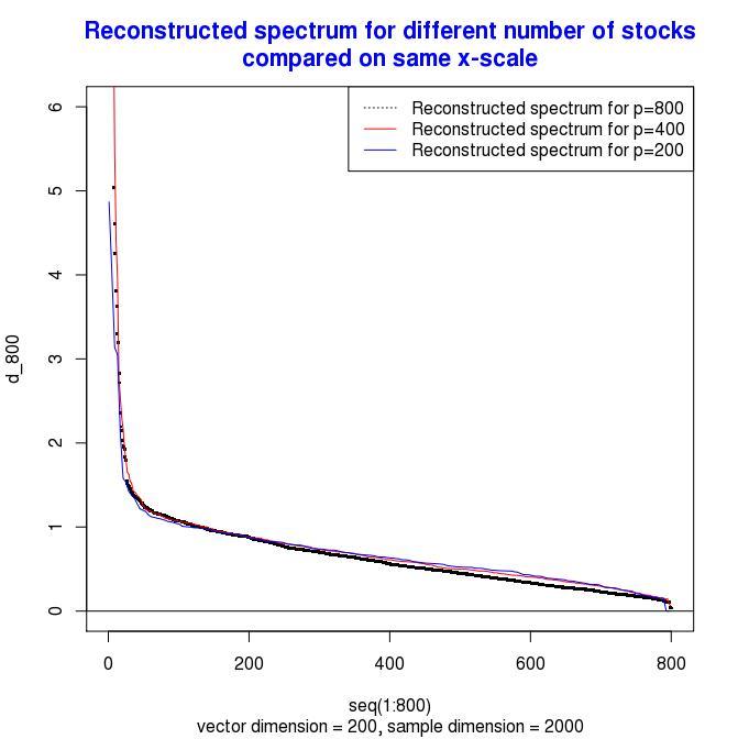
Figure 6: Comparing reconstructed spectrum’s empirical distribution for different numbers p of stocks

Now Figure 6 contradicts the simple model presented in section 1.5. The reason is this. With that model for stocks as being a linear combination of a sector indexes plus an independent firm specific term $\epsilon_{i}$, we would have a fixed number of factors (mainly sectors) which lead to eigenvalues of order $O(p)$. The number of these factors does not change whether we have $400$ or $800$ stocks, since the stocks are chosen at random. In fact, in our actual data there are $11$ sectors. These sectors and a few other factors are responsible for the biggest eigenvalues. (For details about why these eigenvalues are of order $O(p)$ consider our previous example of covariance matrix of stocks $Z,Y,Z,W$ given at the very end of Section LABEL:sectionintro). But, then if the elbow which is seen in the spectrum in Figure 6 would correspond to the transition between the order $O(p)$ eigenvalues and the eigenvalues due to the diagonal, then it should happen at the same index for the $800$ sector data and for the $400$ sector data. By this we mean the same index in absolute terms and not in relative terms. Instead, the elbow is observed at the same relative position, i.e. when we represent the two spectrae above the same $x$-coordinate interval, so as to compare the empirical distribution of the eigenvalues of the restricted and the non-restricted data-sets. The second thing is that the values where the elbow happen are eigenvalues above one. This also contradicts a simple model containing only a number $O(1)$ of order $O(p)$ factors plus the firm independent terms and nothing else. Indeed, according to the model for stocks presented in Section 1.5, apart from the big factors which lead to $O(1)$ eigenvalues of order $O(p)$, the rest of the spectrum should be close to the set $\{VAR[\epsilon_{i}]|i\in 1,\ldots,p\}$. However, since we rescale the stocks so that they have variance $1$, that is we present spectrum of correlation matrix, we have that the variances $VAR[\epsilon]_{i}<1$ if the $\epsilon_{i}$’s are uncorrelated to the factors. This would imply that the eigenvalues which are not order $O(p)$, should be strictly less than $1$.

Let us next see a table with the ratio between the first 30 eigenvalues of the data with $800$ stocks divided by the eigenvalues of the data with $800$ stocks. We present this ratio for the $30$ biggest eigenvalues. The eigenvalues which depend on a factor present in a large part of stocks should grow linearly in $p$. (See subsection LABEL:our_modelling for details as to why). In the table below we see that indeed the biggest eigenvalues are proportional to $p$. So, when we double $p$, these eigenvalues should also approximately double. Hence, the biggest eigenvalue should roughly double as we go from the data with $400$stocks to the data with $800$-stocks. This is indeed the case for the first $14$ eigenvalues as can be seen in the next table:

$$\begin{array}[]{c|c|c|c|c|c|c|c|c|c| c|c|c|c|c|c}\lambda^{800}_{i}/\lambda^{400}_{i}&2.1&2.0&2.0&2.1&1.8&1.9&2.0&1.8&1.7&1.9&1.8&1.9&1.8&1.9&1.7\\ \hline\cr i&1&2&3&4&5&6&7&8&9&10&11&12&13&14&15\end{array}$$

and

$$\begin{array}[]{c|c|c|c|c|c|c|c|c|c| c|c|c|c|c|c}\lambda^{800}_{i}/\lambda^{400}_{i}&1.7&1.6&1.6&1.5&1.4&1.4&1.4&1.4&1.4&1.4&1.2&1.2&1.3&1.3&1.3\\ \hline\cr i&16&17&18&19&20&21&22&23&24&25&26&27&28&29&30\end{array}$$

After eigenvalue $14$, it seems that the linear growth quickly stops as the ratio becomes much smaller than $2$. Now, the elbow in Figure 6 for the data with $800$ stocks happen much after the $14$-th eigenvalue. (At least the lower part of the elbow). This implies that in our data there is more than just a number $O(1)$ of factors present in a large part of the stocks and the firm specific terms, additional to that there must be an order $O(p)$ of “middle size” eigenvalues coming from small number of stocks interactions.

We presented this partial analysis here for one reason. This would not be possible without our reconstruction formula for the spectrum! Indeed, if we do not know the spectrum of the “true” underlying covariance matrix, we can not observe useful facts like for example which eigenvalues grow linearly. Indeed, if you take for your analysis sample covariance matrices spectra, you would not necessarily see that you are dealing with the same spectral distribution for most of the eigenvalues except those of order $O(p)$.

3.3 Big data

Assume that you have a correlation matrix of thousand by thousand. Typically finding all the eigenvalues and eigenvectors goes quite fast, on a personal laptop using $R$. Now, for $10000$ times $10000$ general correlation matrix (not sparse) might be more difficult and we may need to run it for a longer period. Often time, in big data you may have a much bigger dimension than that of $10000$ times $10000$, for example a million times a million. Then, with a classical algorithm and a regular laptop, we can not find all eigenvectors and eigenvalues in short time. Thus, there are some approximation algorithms which can handle much bigger data for finding eigenvectors and eigenvalues. But from experience we know that in certain situations they may not work. However, imagine that by one way or the other for a correlation matrix of a million by a million, we manage to get the sample spectrum. Then, our methods can easily “reconstruct the true underlying spectrum”. How? Well first note that our method with the asymptotic formula for the high dimensional case (formula 1.11), requires only $O(p^{2})$ calculation steps and what is more important only order $O(p)$ working memory. The “curse” with finding eigenvectors for high dimensional correlation matrix when $n$ is of order $O(p)$ is that typically the number of calculation steps is at least of order $O(p^{3})$ and may be larger depending on the size of the spectral gaps. This assuming that the matrix does not have a special structure which makes it easier to compute. So, once we have the spectrum of the sample covariance matrix given to us, our method based on the asymptotic multidimensional formula is very easy to compute even with giant data-sets. What about our fixed point method? Note that method also only requires as input the spectrum of the sample covariance matrix, as well as the two numbers $n$ and $p$. However, that method tries to find a fixed point for a map associated with the second moments of the coefficients of the matrix of eigenvectors of the true covariance matrix expressed in the basis of principal components of the sample covariance, which has to be simulated. More precisely, we have to simulate the data using a first guess of what the spectrum might be in reality. Then for that simulated data, we have to compute all the eigenvectors. And since we want the eigenvectors coefficients second moments, we have to repeat this a few times. This is going to be costly in computational time. This might not be achievable in very high dimension. But, the good news is that we can scale things down. That is if you are given $n$ and $p$ simply solve the problem for much smaller data set where the ratio $n/p$ remains the same and where you take approximately the same empirical distribution of the sample covariance spectrum. Once, you find in this way the reconstructed spectrum you scale it up and you get almost the exact answer. In the example below this is what we did: we divided $n$ and $p$ by a factor $5$. The big data was $2000$ days and $800$ stocks. Then, we simulate a data-set which is $5$ times in the number of samples and the size of vector. That is we simulate a data set which would correspond to $160$ stocks and $400$ days. We took for this a five times dimension reduced spectrum from the full sample covariance. That is we took the full data sample spectrum. Then we produced a spectrum on a dimension five times less, so that the new spectrum would have approximately the same empirical distribution. (Notice that we did not scale down the real life data, but only the sample spectrum). Then, we do simulations for our reconstruction on the reduced dimensional space. The resulting reconstruction is then presented on the same scale as the higher dimension reconstruction. The result can be seen in the next figure below (see Figure 6, where we compare the reconstructed on the full data, versus the reconstructed on the scaled down data by a factor $5$. We see that the scaled down reconstruction does an almost perfect job in reconstructing the “true higher dimensional spectrum”. Again, here we did not scale down the data, but only the reconstruction process! This means that from the given full spectrum of the sample covariance matrix, we scale down by taking a spectrum with basically approximately same empirical distribution but vectors on a five times smaller dimension. Then, we did the fixed point eigenvector reconstruction on that smaller space. The result is shown again in the higher dimensional plot, but showing the obtained empirical spectrum on the right scale so that it can be compared to the reconstructed spectrum at full scale. And indeed we got perfect match. Note that we had to adjust the 5 biggest eigenvalues a little bit, to obtain the result.

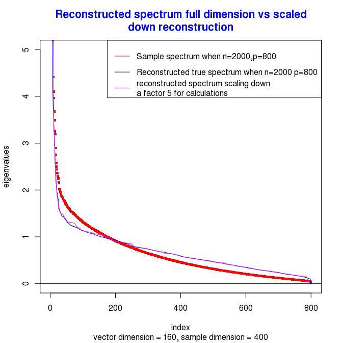
Figure 7: Reconstruction from full sample spectra, scaled down to a lower dimensional space, a simulations for reconstruction done in lower dimensional space

4 Testing the different methods numerically

In real data we have always observed spectrae which look continuous and highly convex. But in the model in section 1.5, the stocks were written as linear combination of factors and the part which comes only from the firm. Thus in theory according to such a model, we would have a small number of order $O(1)$ of eigenvalues of order $O(p)$. The rest of the eigenvalues would be of order $O(1)$. In reality, this is never what we have seen in real-life data. Instead, we have a continuum going from the biggest eigenvalues to the eigenvalues of order $O(1)$. Indeed there is often, one eigenvalue (or a very small number) which is separated from the rest. After this largest eigenvalue (or couple of them) we don’t go directly to something which is order $O(1)$ and does not grow, but instead have a continuum of eigenvalues among which some grow as we increase $p$ and hence are not of order $O(1)$. Hence, to evaluate our spectrum reconstructing methods, we are primarily interested in such spectrum with the properties we encounter mostly in real data, that is, “continous functions except mabye for the biggest eigenvalue (or maybe an very small number of eigenvalues)” and the rest of the eigenvalues having the function $s\mapsto\lambda_{s}$ looking continuous convex and with derivative going to $-\infty$ as the index goes to $0$. Recall that the eigenvalues of $E[Z^{t}Z]$ are denoted by $\lambda_{1}>\lambda_{2}>\ldots>\lambda_{o}$.

In our subsequent simulations, we often take a relatively small dimension with $p=100$ for example. Why? To make simulations quicker and because we have seen that even if you blow up things from there things do not change too much. In Figure 2 we see what happens when we take $n$ and $p$ both $100$ times bigger, but we take about the same empirical distribution for the spectrum of the original covariance matrix $COV[\vec{X}]$. The empirical distribution of the estimated covariance matrix $\widehat{COV}[\vec{X}]$ barely changes. Thus, to test the different recovering methods, a low dimension like $p=100$ should be enough in practice when dealing with synthetic data. With real life data, things are very different, and we also need to test our method with large $p$. Indeed, when $p$ becomes larger, the real spectrum of the underlying covariance matrix does not have approximately apriori the same distribution, since the biggest eigenvalues are supposed to grow linearly in $p$!

Another important thing, would be to distinguish between those spaectrae (of underlying covariance matrix) which are strongly bounded away from $0$ (like $\lambda_{s}\geq 0.3$ for example in stocks) and the others like in futures, where there a close to $0$ eigenvalues, reflecting the possibility of arbitrage. Indeed if the true spectrum is bounded away from zero say for example by $0.3$, then a good measure for comparing how well the different reconstruction methods work, would be to take the maximum of relative error:

$$\max_{s=1,\ldots,p}\frac{|\lambda_{s}-\widehat{\lambda}_{s}^{M}|}{\lambda_{s}},$$

where $\widehat{\lambda}_{s}^{M}$ is the estimate of the $s$-th eigenvalue $\lambda_{s}$ using the estimation method $M$. If there are eigenvalues $\lambda_{s}$ close to zero we need to use another method to access the precision of the reconstruction method as in that case the relative error for the values $\lambda_{s}$ close to $0$ is meaningless. So, for that case we will take the maximum of the relative error only for those $\lambda_{s}$ which are bigger than $0.2$. For those which are smaller we take the maximum absolute error.

4.1 Testing our methods on synthetic multivariate normal data

We simulate multivariate normal data using various spectrum: linear, two different linear segments combined, step function and spectrum from stock data. In particular, we compare our eigenvector method with Quest provided by the free probability approach [12].

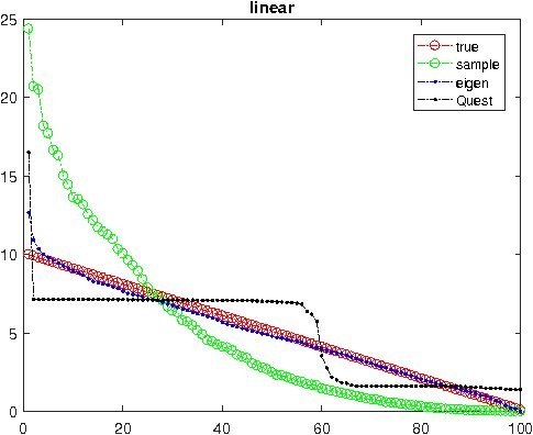
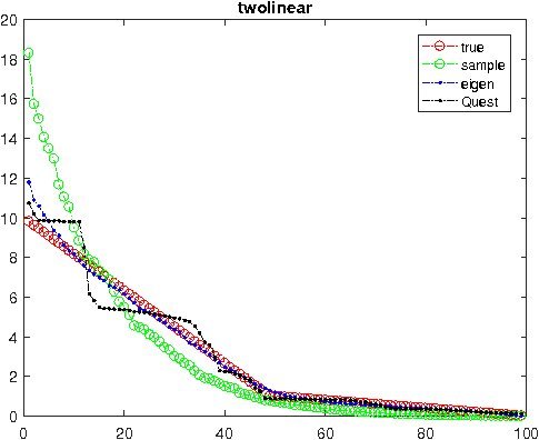
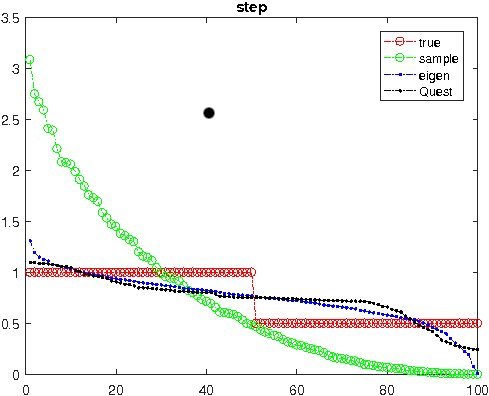
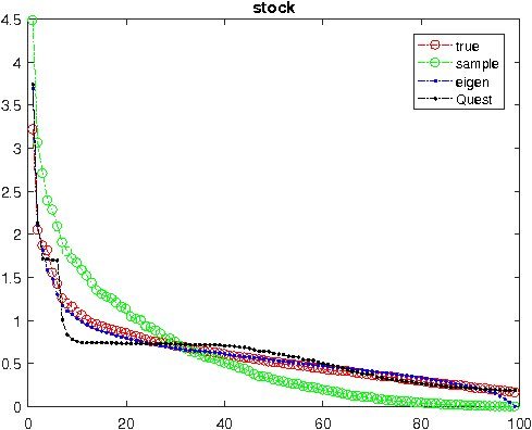
Figure 8:

In the majority of those cases Figure 8, eigenvector approach outperform others. There is another significant advantage of eigenvector approach. That is its insensitivity to the sample spectrum, where Quest varies quite significantly even when sample spectrum exhibits a small change. In other words, when a different sample matrix is given, the recovery of our eigenvector method does not fluctuate, which means the variance is small.

For a totally flat spectrum the first method does not work well: This is not too surprising since our first method is based on comparing the $i$-th eigenvector of the sample covariance matrix with the $i$-th eigenvector of the true covariance. In the flat spectrum case, all eigenvectors of the true covariance matrix are identical. This can be seen in figure 9 below.

Figure 9: First method fails, second not very precise for constant spectrum.

Also, often by scaling down and then retrieving the spectrum for the smaller data, set we can retrieve the true spectrum. This is shown in Figure 10.

Figure 10: By scaling down and then reconstructing before blowing up again, we manage to retrieve the spectrum for big data.

References

- [1] Z. D. Bai and Y. Q. Yin. Convergence to the semicircle law. Ann. Probab., 16(2):863–875, 04 1988.
- [2] Zhidong Bai, Jiaqi Chen, and Jianfeng Yao. On estimation of the population spectral distribution from a high-dimensional sample covariance matrix. Australian and New Zealand Journal of Statistics, 52(4):423–437, 2010.
- [3] Peter J. Bickel and Elizaveta Levina. Regularized estimation of large covariance matrices. Ann. Statist., 36(1):199–227, 2008.
- [4] Z. Burda, A. Görlich, A. Jarosz, and J. Jurkiewicz. Signal and noise in correlation matrix. Phys. A, 343(1-4):295–310, 2004.
- [5] Noureddine El Karoui. Spectrum estimation for large dimensional covariance matrices using random matrix theory. Ann. Statist., 36(6):2757–2790, 12 2008.
- [6] Noureddine El Karoui et al. Spectrum estimation for large dimensional covariance matrices using random matrix theory. The Annals of Statistics, 36(6):2757–2790, 2008.
- [7] Matan Gavish and David L. Donoho. Optimal shrinkage of singular values. IEEE Trans. Inform. Theory, 63(4):2137–2152, 2017.
- [8] Vladimir Koltchinskii and Karim Lounici. Asymptotics and concentration bounds for bilinear forms of spectral projectors of sample covariance. Ann. Inst. Henri Poincaré Probab. Stat., 52(4):1976–2013, 2016.
- [9] Vladimir Koltchinskii and Karim Lounici. Concentration inequalities and moment bounds for sample covariance operators. Bernoulli, 23(1):110–133, 2017.
- [10] Vladimir Koltchinskii and Karim Lounici. Normal approximation and concentration of spectral projectors of sample covariance. Ann. Statist., 45(1):121–157, 2017.
- [11] W. Kong and G. Valiant. Spectrum estimation from samples. Annals of Statistics, 45(5):2218–2247, 2017.
- [12] Olivier Ledoit and Michael Wolf. Nonlinear shrinkage estimation of large-dimensional covariance matrices. Ann. Statist., 40(2):1024–1060, 04 2012.
- [13] Olivier Ledoit and Michael Wolf. Spectrum estimation: A unified framework for covariance matrix estimation and pca in large dimensions. Journal of Multivariate Analysis, 139(Supplement C):360 – 384, 2015.
- [14] Olivier Ledoit and Michael Wolf. Spectrum estimation: A unified framework for covariance matrix estimation and pca in large dimensions. Journal of Multivariate Analysis, 139:360–384, 2015.
- [15] Olivier Ledoit, Michael Wolf, et al. Nonlinear shrinkage estimation of large-dimensional covariance matrices. The Annals of Statistics, 40(2):1024–1060, 2012.
- [16] Weiming Li, Jiaqi Chen, Yingli Qin, Zhidong Bai, and Jianfeng Yao. Estimation of the population spectral distribution from a large dimensional sample covariance matrix. Journal of Statistical Planning and Inference, 143(11):1887 – 1897, 2013.
- [17] V A Marčenko and L A Pastur. Distribution of eigenvalues for some sets of random matrices. Mathematics of the USSR-Sbornik, 1(4):457, 1967.
- [18] J.W. Silverstein. Strong convergence of the empirical distribution of eigenvalues of large dimensional random matrices. Journal of Multivariate Analysis, 55(2):331 – 339, 1995.
- [19] C Stein. Estimation of a covariance matrix. Ritz lecture at annual IMS meeting in Atlanta 1975, 1975.
- [20] Dan Voiculescu. Limit laws for random matrices and free products. Inventiones mathematicae, 104(1):201–220, 1991.
- [21] Dan V Voiculescu, Ken J Dykema, and Alexandru Nica. Free random variables. Number 1. American Mathematical Soc., 1992.
- [22] Y.Q Yin, Z.D Bai, and P.R Krishnaiah. Limiting behavior of the eigenvalues of a multivariate f matrix. Journal of Multivariate Analysis, 13(4):508 – 516, 1983.