Observational constraints on Quintessence models of dark energy

Abstract

Scalar fields aptly describe equation of state of dark energy. The scalar field models were initially proposed to circumvent the fine tuning problem of cosmological constant. However, the model parameters also need a fine tuning of their own and it is important to use observations to determine these parameters. In this paper, we use a combination of low redshift data to constrain the of canonical scalar field parameters. For this analysis, we use the Supernova Type Ia Observations, the Baryon Acoustic Observations and the Hubble parameter measurement data. We consider scalar field models of the thawing type of two different functional forms of potentials. The constraints on the model parameters are more stringent than those from earlier observations although these datasets do not rule out the models entirely. The parameters which let dark energy dynamics closely emulate that of a cosmological constant are preferred. The constraints on the parameters are suitable priors for further quintessence dark energy studies.

1 Introduction

The discovery of late time cosmic acceleration by the Supernova Type Ia observations has been one of the most important results in cosmology [1, 2]. Nearly two-thirds of the energy of the universe is due to the cosmological constant or an alternative description called the dark energy[3]. The presence of dark energy has been further confirmed by many different observations such as Baryon Acoustic Oscillations [4] and Cosmic Microwave Background observations [5, 6]. More recently, data from direct measurements of the Hubble parameter has also shown to be a useful probe of low redshift evolution of the universe [7, 8, 9].

Dark energy can be modeled by invoking the presence of a cosmological constant model for which the value of the equation of state parameter is $w=-1$ [10, 11] and this model is consistent with observational data [12, 13, 14]. Einstein’s cosmological constant $\Lambda$ is attributed to the zero-point energy of the vacuum, with a constant energy density $\rho$, a negative pressure $P$ with an equation of state given by $w\equiv P/\rho=-1$. Observations do, however, allow a $w$ which is different from that of a cosmological constant and has a dynamical nature i.e. it varies with time. The variation with time is achieved by extending the description of barotropic fluid equation of state parameter to be a function of time or the scale factor. A few parameterisations which have been proposed are described in [15, 16] and there are non baroptropic fluids such as the Chaplygin gas in [17].

A slowly varying scalar field have been proposed to be a viable substitute for the cosmological constant as the negative equation of state parameters arises naturally in these scenarios. The scalar field models include those based on canonical scalar field matter such as the quintessence [18, 19, 20, 21, 22, 23, 24], kinetic energy driven k-essence [25, 26] and others like tachyon [27, 28]. There is at present no consensus as to which of these models better describe dark energy. Although proposed to do away with the fine tuning problem of the cosmological constant, the scalar field models have fine tuning requirements of their own. The potential parameters need to be fine tuned such that the acceleration of the universe begins after a sufficiently long matter dominated era in order that the large scale structures form. Among the models listed above, the quintessence model is described by a canonical scalar field. For a slowly varying field, the scalar field potential model universe has a positive acceleration.

Since a large amount of data is now available and there is a large variety of observations, it is possible to constrain cosmological parameters to to better precision than before. This is especially true of observations which have constraints orthogonal to each other and hence the combined range is much smaller than that allowed by individual datasets. Many observations such as supernovae (SNIa) data [1, 2, 29, 30, 31, 32, 33, 34, 35], Baryonic Acoustic oscillation (BAO) data [4, 36, 37, 38, 39, 40, 41] and Hubble distance (H(z)) measurements using different methods by [37, 38, 42, 43, 44, 45, 46, 47, 7], compiled in [7, 8, 9] can be used for constraining models.

In this work, we revisit the quintessence dynamics in the light of more recent and diverse cosmological observations. We restrict ourselves to low redshift, distance measurement data. The main motivation in this work is to study the present constraints with a view to reduce the priors. We consider different quintessence scenarios, with different scalar field potentials. These different scenarios have been broadly classified as thawing and freezing type [48, 49, 50, 51, 52, 53]. This broad classification is based on the whether the equation of state parameters is cosmological constant like in the past, or if this behaviour is at later time. While it may be expected that the equation of state parameter can be effectively constrained by assuming dark energy to be a fluid, it is important to explicitly study different scalar field models. The equation of state parameter depends on the time evolution of the scalar field and the functional form of the scalar field potential. In this work, we determine constraints on the equation of state parameters for different thawing scalar field models. Earlier similarly motivated studies include [54, 55, 56, 57, 58, 59, 60, 61, 62, 63, 64, 65, 66]. Structure formation in dark energy scenarios has also been studied in [67, 68, 69, 70, 71, 72]. Recent study shows that the scalar fields fir observations better than the $\Lambda$CDM model, but the difference is not significant [73].

This paper is structured as follows. After introduction in section 1, in section 2, we discuss cosmological equations for quintessence scalar field model. In section 3, we show the solutions of the equations for different potentials. The key results are discussed in section 4 and we summarize and conclude in section 5.

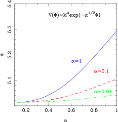
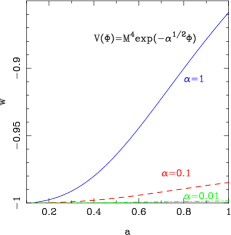
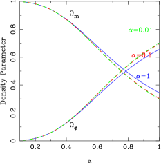
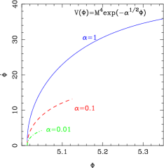
Figure 1: The plots in the figure represent evolution of different quantities corresponding to the potential $V(\phi)=M^{4}exp(-\alpha^{1/2}\phi/M_{p})$. We consider three different values of $\alpha=0.01,~{}0.1$ and $~{}1$ and we have rescaled the variable $\phi$ as $\Phi=\phi/M_{p}$. In the first row, the plot on the left shows the variation of $\Phi$ as a function of scale factor for different values of $\alpha$. The plot on the right shows the behavior of equation of state parameter $w$ as the scale factor varies. In the second row, the plot on the left is for energy density parameter of the field and matter and the figure on the right is the phase plot for the exponential potential. Here, the solid curve represents results for $\alpha$=1, the dashed curve is drawn for $\alpha$=0.1 and the dot-dashed curve is for $\alpha$=0.01.

Potential	Parameter	Lower Limit	Upper Limit
$V(\phi)=M^{4}e^{(-\alpha^{1/2}\phi/M_{p})}$	$\Omega_{m}$	0.01	0.6
	$w_{0}$	-1.0	1.0
	$\alpha$	0.01	190.0
$V(\phi)=M^{4-n}\phi^{n}$	$\Omega_{m}$	0.01	0.6
	$w_{0}$	-1.0	1.0
	$\phi_{in}$	1.0	10.0

Table 1: This table lists the priors used for parameter fitting in case of both the potentials.

2 Quintessence Dynamics

We consider a canonical scalar field $\phi$ minimally coupled, i.e. experiencing gravity passively through the spacetime curvature and a self-interaction described by the scalar field potential V($\phi$) and with a canonical kinetic energy contribution. The action for a quintessence field is therefore given by

$$S=\int d^{4}x\sqrt{-g}\begin{pmatrix}-\frac{1}{2}(\nabla\phi)^{2}-V(\phi)\end{pmatrix}$$ (2.1)

where

$$(\nabla\phi)^{2}=g^{\nu\mu}\partial_{\nu}\phi\partial_{\mu}\phi$$ (2.2)

In a flat Friedmann background, the pressure and energy density of a homogeneous scalar field are given by

$$P=\frac{\dot{\phi}^{2}}{2}-V(\phi)$$ (2.3)

$$\rho=\frac{\dot{\phi}^{2}}{2}+V(\phi).$$

The equation of state, which in general is time varying, is defined as

$$w=\frac{P}{\rho}.$$ (2.4)

The equation of motion for the scalar field, the Klein-Gordon equation takes the form

$$\ddot{\phi}+3H\dot{\phi}=-\frac{dV}{d\phi},$$ (2.5)

follows from functional variation of the Lagrangian and is interchangeable with the continuity equation.

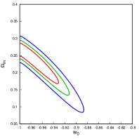
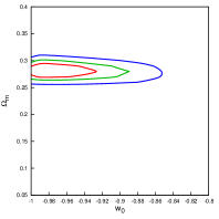
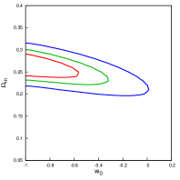
Figure 2: The figure represents $1\sigma$, $2\sigma$ and $3\sigma$ confidence contours in $w_{0}-\Omega_{m}$ plane for the thawing potential $V=M^{4}\exp(-\sqrt{\alpha}\Phi)$. From left to right, the plot are for the SNIa, BAO and H(z) data respectively. Here, we have marginalised over the parameter $\alpha$.

Data set	$3\sigma$ confidence	$\chi_{m}^{2}$	Best Fit Model
$V=M^{4}\exp(-\sqrt{\alpha}\Phi)$
SNIa	-1.0$\leq$ $w_{0}$ $\leq$-0.63		$w_{0}$=-0.97
	0.01$\leq$ $\Omega_{m}$ $\leq$0.31	563.42	$\Omega_{m}$=0.24
	0.01$\leq$ $\alpha$ $\leq$1.0		$\alpha$=0.03
BAO	-1.0$\leq$ $w_{0}$ $\leq$-0.85		$w_{0}$=-0.99
	0.26$\leq$ $\Omega_{m}$ $\leq$0.31	2.35	$\Omega_{m}$=0.28
	0.01$\leq$ $\alpha$ $\leq$ 1.0		$\alpha$=0.07
H(z)	-1.0$\leq$ $w_{0}$ $\leq$0.14		$w_{0}$=-1.0
	0.19$\leq$ $\Omega_{m}$ $\leq$0.32	17.04	$\Omega_{m}$=0.26
	0.01$\leq$ $\alpha$ $\leq$1.0		$\alpha$=1.0

Table 2: The above table shows the 3$\sigma$ confidence limit for all the three data for the potential $V=M^{4}\exp(-\sqrt{\alpha}\Phi)$ and the value of the parameters corresponding to minimum value of $\chi^{2}$ for the exponential potential.

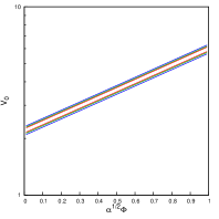
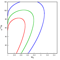
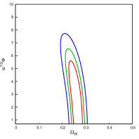
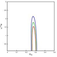
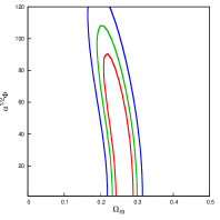
Figure 3: The figure represents $1\sigma$, $2\sigma$ and $3\sigma$ confidence contours in $\sqrt{\alpha}\Phi-V_{0}$ plane for the exponential potential $V=M^{4}\exp(-\sqrt{\alpha}\Phi)$ in the first row. Here, $V_{0}$ is scaled by the square of the present value of Hubble parameter ($H_{0}^{2}$). The plots in second row represents confidence contours in $w_{0}-\sqrt{\alpha}\Phi$ plane and contours in plane $\Omega_{m}-\sqrt{\alpha}\Phi$ are given in third row. The scheme of the plots is same as in figure 2.

The evolution of a spatially flat universe is described by Friedmann equations,

$$H^{2}=\left(\frac{\dot{a}}{a}\right)^{2}=\frac{8\pi G\rho}{3}$$ (2.6)

$$\frac{\ddot{a}}{a}=-\frac{4\pi G}{3}(\rho+3P)$$ (2.7)

where $H$ is the Hubble parameter, $\rho$ and $P$ denote the total energy density and pressure of all the components present in the universe at a given epoch. Using equation (2.3) yields

$$H^{2}=\frac{8\pi G}{3}\left[\frac{1}{2}\dot{\phi}^{2}+V(\phi)\right],$$ (2.8)

$$\frac{\ddot{a}}{a}=-\frac{8\pi G}{3}\left[\dot{\phi}^{2}-V(\phi)\right].$$ (2.9)

For an accelerating universe $\dot{\phi}^{2}<V(\phi)$. This implies that one requires an almost flat potential for an accelerated expansion. The equation of state for the scalar field $\phi$ is given by

$$w=\frac{\dot{\phi}^{2}-2V(\phi)}{\dot{\phi}^{2}+2V(\phi)}.$$ (2.10)

Depending on the evolution of $w$, different quintessence models are classified into two broad categories [55, 56, 58, 74, 75, 76, 77, 78, 79]. The first corresponds to thawing models, in which the field is nearly frozen by a Hubble damping during the early cosmological epoch and it starts to evolve at late times. Here the field is displaced from its frozen value recently, when it starts to roll down to the minimum. In this case, the evolution of $w$ is characterised by the growth from $-1$, at early times the equation of state is $w\approx$ -1, but grows less negative with time. We analyse the following concave potentials for thawing behaviour [80, 81, 82, 83, 84].

• Exponential potential [22, 85, 86, 87, 88]:

  $$V=M^{4}\exp(-\sqrt{\alpha}\phi/M_{p})$$ (2.11)

• Polynomial (concave) potential :

  $$V=M^{4-n}\phi^{n}.$$ (2.12)

For the potential described by a polynomial, we consider $n=1,2,3$. These different values correspond to potentials with different shapes. The other class of potentials consists of a field which was already rolling towards minimum of its potential, prior to the onset of acceleration, but slows down because of the shallowness of the potential at late times and comes to a halt as it begins to dominate the universe. For freezing models, the equation of state parameter $w$ approaches $-1$. For this work, we will focus on homogeneous scalar fields belonging to thawing class.

3 Solutions to cosmological equations

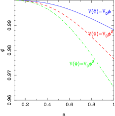
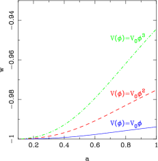
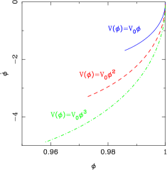
Figure 4: The plots in this figure represent the theoretical results obtained for potential $V(\phi)=M^{4-n}\phi^{n}$, for $n$ =1, 2 and 3. In this figure, the solid line represents results for $n=1$, dashed curve is drawn for quadratic potential, $n=2$ and dotted-dashed curve is for cubic power potential, $n=3$. In the first row, the plot on the left shows the variation of $\phi$ as a function of scale factor. The figure on the right shows the evolution of equation of state parameter $w$ for the potential as scale factor changes. In the second row, the plot on the left is for variation of energy density parameter for the field ($\Omega_{\phi}$) and matter ($\Omega_{m}$) as a function of scale factor and the figure on the right is the phase plot for the power potential.

n	SnIa data	BAO data	H(z) data
1	$\chi^{2}_{min}=608.61$	$\chi^{2}_{min}=2.29$	$\chi^{2}_{min}=17.06$
	$w_{0}=-0.98$	$w_{0}=-1.0$	$w_{0}=-1.0$
	$\Omega_{m}=0.21$	$\Omega_{m}=0.28$	$\Omega_{m}=0.27$
	$\phi_{in}=1.7$	$\phi_{in}=10.0$	$\phi_{in}=3.1$
2	$\chi^{2}_{min}=608.59$	$\chi^{2}_{min}=2.41$	$\chi^{2}_{min}=17.06$
	$w_{0}=-0.98$	$w_{0}=-1.0$	$w_{0}=-1.0$
	$\Omega_{m}=0.22$	$\Omega_{m}=0.28$	$\Omega_{m}=0.27$
	$\phi_{in}=6.2$	$\phi_{in}=10.0$	$\phi_{in}=5.8$
3	$\chi^{2}_{min}=608.54$	$\chi^{2}_{min}=2.65$	$\chi^{2}_{min}=17.05$
	$w_{0}=-0.98$	$w_{0}=-1.0$	$w_{0}=-1.0$
	$\Omega_{m}=0.21$	$\Omega_{m}=0.28$	$\Omega_{m}=0.27$
	$\phi_{in}=5.5$	$\phi_{in}=10.0$	$\phi_{in}=8.4$

Table 3: The above table shows the value of the parameters corresponding to minimum value of $\chi^{2}$ for the potential $V=M^{4-n}\phi^{n}$ .

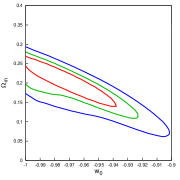
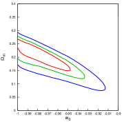
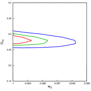
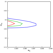
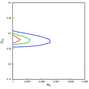
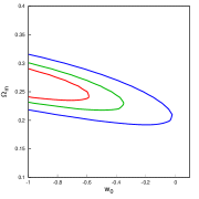
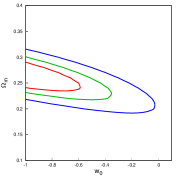
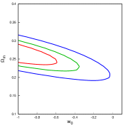
Figure 5: The plots in this figure are confidence contours in $\Omega_{m}-w_{0}$ plane for the potential $V=V_{0}\phi^{n}$. In first row, from left to right, the plots are for SNIa data with $n=1,2,3$ respectively. In the second row, the plots are for BAO data and the third row shows the plots for the H(z) data.

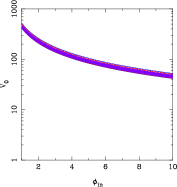
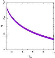
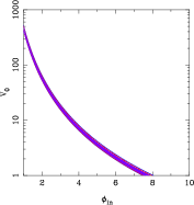
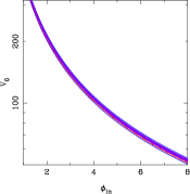
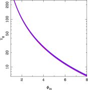
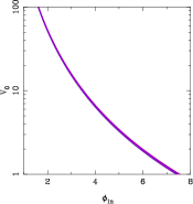
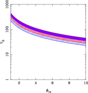
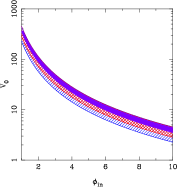
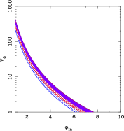
Figure 6: The plots in the rows of the figure represent allowed region for $V_{0}=M^{4-n}$ corresponding to $1\sigma$, $2\sigma$ and $3\sigma$ confidence region as a function of field $\phi_{in}$, for $V=V_{0}\phi^{n}$. Going from left to right, the first, second and third plots are obtained for potentials corresponding to $n$ equal to $1$, $2$ and $3$ respectively. In first row, the plots shows results for SNIa, the plots in second row are obtained for BAO data and the third row shows the plots for H(z) dataset. The solid blue region in the middle shows the allowed range of $V_{0}$ at $1\sigma$ level, the red hatched region corresponds to $2\sigma$ level and the region with blue slanted lines shows the $3\sigma$ range. The white region is ruled out.

n	SNIa data	BAO data	H(z) data
1	-1.0$\leq$ $w_{0}$ $\leq$-0.92	-1.0$\leq$ $w_{0}$ $\leq$-0.995	-1.0$\leq$ $w_{0}$ $\leq$0.1
	0.1$\leq$ $\Omega_{m}$ $\leq$0.29	0.26$\leq$ $\Omega_{m}$ $\leq$0.31	0.19$\leq$ $\Omega_{m}$ $\leq$0.32
	1.0$\leq$ $\phi_{in}$ $\leq$10.0	1.0$\leq$ $\phi_{in}$ $\leq$ 10.0	1.0$\leq$ $\phi_{in}$ $\leq$ 10.0
2	-1.0$\leq$ $w_{0}$ $\leq$-0.91	-1.0$\leq$ $w_{0}$ $\leq$-0.996	-1.0$\leq$ $w_{0}$ $\leq$0.1
	0.1$\leq$ $\Omega_{m}$ $\leq$0.29	0.26$\leq$ $\Omega_{m}$ $\leq$0.31	0.18$\leq$ $\Omega_{m}$ $\leq$0.32
	1.0$\leq$ $\phi_{in}$ $\leq$10.0	1.9$\leq$ $\phi_{in}$ $\leq$ 10.0	1.0$\leq$ $\phi_{in}$ $\leq$ 10.0
3	-1.0$\leq$ $w_{0}$ $\leq$-0.91	-1.0$\leq$ $w_{0}$ $\leq$-0.997	-1.0$\leq$ $w_{0}$ $\leq$0.08
	0.1$\leq$ $\Omega_{m}$ $\leq$0.29	0.26$\leq$ $\Omega_{m}$ $\leq$0.31	0.18$\leq$ $\Omega_{m}$ $\leq$0.32
	1.0$\leq$ $\phi_{in}$ $\leq$10.0	2.8$\leq$ $\phi_{in}$ $\leq$ 10.0	1.0$\leq$ $\phi_{in}$ $\leq$ 10.0

Table 4: The above table shows the 3$\sigma$ confidence limit for all the three data for the potential $V=V_{0}\phi^{n}$ for n=1,2,3.

In this section, we discuss the background cosmology and numerical solutions for the different types of potentials that we have discussed in the previous section.

3.1 The exponential potential

To study how the universe evolves in the presence of this potential, we solve the Klein-Gordon equation, equation (2.5), and Friedmann equations for the scalar field, equation (2.8). In order to solve the equations, we define the following dimensionless variable:

$$\Phi=\frac{\phi}{M_{p}}.$$ (3.1)

The potential, then, takes the form

$$V(\Phi)=M^{4}\exp({-\sqrt{\alpha}\Phi}).$$ (3.2)

In terms of the new variables, the cosmological equations can be written as

$$\ddot{\Phi}+3\frac{\dot{a}}{a}\dot{\Phi}-\sqrt{\alpha}V_{0}\exp(-\sqrt{\alpha}\Phi)=0,$$ (3.3)

$$\left(\frac{\dot{a}}{a}\right)^{2}=H_{0}^{2}\frac{\Omega_{m}}{a^{3}}+\frac{\dot{\Phi}^{2}}{6}+\frac{V_{0}}{3}\exp(-\sqrt{\alpha}\Phi)$$

where $V_{0}=\frac{M^{4}}{M_{p}^{2}}$ and $H_{0}$ is the present value of Hubble parameter. For $\Omega_{total}=\Omega_{m}+\Omega_{\phi}=1$, the initial conditions are given by

$$V_{0}=\frac{3H_{0}^{2}}{2}(1-\Omega_{m_{i}})(1-w_{in})\exp(\sqrt{\alpha}\Phi_{in})$$ (3.4)

$$\dot{\Phi}_{in}^{2}=3H_{0}^{2}(1-\Omega_{m_{i}})(1+w_{in});\hskip 14.22636pt\Phi_{in}=1.$$ (3.5)

The variables $\Omega_{m_{i}}$, $\Phi_{in}$ and $w_{in}$ are values of non-relativistic matter density parameter, field and equation of state parameter at some initial time $t=t_{i}$ (and $w_{0}$ represents the present day value of $w$).

By solving these coupled equations numerically, we solve for $\Phi$ and $\dot{\Phi}$ as a function of the scale factor. These values are, then, used to determine the value of equation of state parameter $w$, which in terms of the dimensionless parameters is given by

$$w=\frac{{\dot{\Phi}}^{2}-2V_{0}\exp(-\sqrt{\alpha}\Phi)}{{\dot{\Phi}}^{2}+2V_{0}\exp(-\sqrt{\alpha}\Phi)}.$$ (3.6)

From the above equation we can see that, depending upon the form of potential $V(\Phi)$, $w$ lies between $-1$ and $+1$.

To study the evolution of the model, we evolve the system from early time to late time. We plot the results obtained for this potential in figure 1. The plot on the left in the first row shows the variation of $\Phi$ as a function of scale factor (past to future). The plot on the right shows the behaviour of equation of state parameter $w$ as scale factor changes. In the second row, the plot on left is for energy density of the field as a function of scale factor and the figure on the right is the phase plot obtained for the model.

3.2 The Polynomial (concave) potential

The second potential of thawing class that we analysed is a power potential given by

$$V(\phi)=M^{4-n}\phi^{n}.$$ (3.7)

The background equations then take the following form:

$$\ddot{\phi}+3\frac{\dot{a}}{a}\dot{\phi}+nV_{0}{\phi}^{n-1}=0,$$ (3.8)

$$\left(\frac{\dot{a}}{a}\right)^{2}=\frac{\Omega_{m}}{a^{3}}+\frac{\dot{\phi}^{2}}{6}+\frac{V_{0}{\phi}^{n}}{3}.$$

And equation of state becomes

$$w=\frac{{\dot{\phi}}^{2}-2V_{0}{\phi}^{n}}{{\dot{\phi}}^{2}+2V_{0}{\phi}^{n}}.$$ (3.9)

The value of $V_{0}$ for this potential is found to be

$$V_{0}=\frac{3H_{0}^{2}}{16\pi G}(1-\Omega_{m_{i}})(1-w_{in})\phi^{-n}_{in}$$ (3.10)

and the initial value of field velocity, $\dot{\phi}_{in}$ is given by

$$\dot{\phi}_{in}=\pm\sqrt{\frac{3H_{0}^{2}}{8\pi G}(1-\Omega_{m_{i}})(1+w_{in})}.$$ (3.11)

As mentioned earlier, to study this potential, we consider $n=1,2,3$, corresponding to different background evolution.

We plot the results obtained by evolving the system from past to present and then to future for this potential in figure 4. In the first row, the plot on left shows the variation of $\phi$ as a function of scale factor. The next plot shows the behaviour of equation of state parameter $w$ for the potential with respect to scale factor, $a$. In the second row, the plot on left is for energy density of the field as a function of $a$ and the second figure is the phase plot obtained for the polynomial potential.

4 Observational constraints on parameters

In this section, we discuss the results obtained by using the three different cosmological observations in the analysis. For the data analysis we use the $\chi^{2}$ minimisation technique. The observational data consists of $n$ points of observables ($X_{n,ob}$), such as luminosity distance for supernova data or angular diameter distance for the BAO data, at a particular redshift ($z_{n}$), along with error associated with the observable ($\sigma_{n}$). In this technique, we calculate the same observable quantity ($X_{n,th}$) at the same redshift, with the equation state parameter obtained by solving cosmological equations in the presence of scalar field with a particular potential $V(\phi)$. The $\chi^{2}$ measures the goodness of fit i.e., by how much the observational value differs in comparison to theoretically expected value and is defined as

$$\chi^{2}=\sum_{k}\left[\frac{X_{k,ob}-X_{k,th}}{\sigma_{k}}\right]^{2}$$ (4.1)

We have listed the priors used for the analysis in table 1.

For the exponential potential, $V(\phi)=M^{4}\exp(-\sqrt{\alpha}\phi/M_{p})$, the free parameters are the dark energy equation of state parameter $w_{0}$, matter density parameter $\Omega_{m}$ and $\alpha$ in combination with the present day value of $\phi/M_{p}$, where $M_{p}$ is the Plank mass. In figure 2, we show the $1\sigma$, $2\sigma$ and $3\sigma$ confidence contours in $\Omega_{m}-w_{0}$ plane. Here, $\Omega_{m}$ and $w_{0}$ denote the present day value of non-relativistic matter density parameter and present day dark energy equation of state parameter. The plot on the left is from SNIa data, the plot in the middle is for BAO data and the plot on the right shows the results from H(z) data. To obtain the contours we have marginalised over the entire range of the third parameter $\alpha$. The minimum value of $\chi^{2}$ ($\chi^{2}_{min}$) and the constraints obtained for the parameters are listed in table 2. BAO data provides the narrowest constraints on $\Omega_{m}$ and on the upper limit of $w_{0}$; none of the data sets provide a lower limit on $w_{0}$. The Hubble data constrains $\Omega_{m}$ strongly but it allows the regions of $w_{0}$ within $3\sigma$ limits, which gives decelerated expansion. Supernovae data allows the maximum range in $\Omega_{m}$; between $\Omega_{m}=0.08$ to $0.31$ and the range of $w_{0}$ below $w\leq-0.87$, and it does not allow for a decelerated expansion of the universe.

In the first row of figure 3, we present the confidence contours corresponding to $1\sigma$, $2\sigma$ and $3\sigma$ levels in $V_{0}$ and $\sqrt{\alpha}\Phi$ plane. Here, we show the results for the range $0-1$ of $\sqrt{\alpha}\Phi$. We find that the most stringent constraints are provided for BAO dataset, and the widest range is allowed for H(z) data and for SNIa dataset the range lies between the range provided by other two datasets. In figure 3, we show the allowed range of $\sqrt{\alpha}\Phi$ and $w_{0}$ for different datasets in second row and in third row we show the constraints on $\sqrt{\alpha}\Phi$ versus $\Omega_{m}$. The first plot is obtained for SNIa, second plot is obtained for BAO and third plot is the result from H(z) data respectively. The results are consistent with the confidence contours of Fig. 2, this is because the value of $V_{0}$ depends upon both $\Omega_{m}$ and $w_{0}$.

We now discuss the results obtained for the exponential potential, $V(\phi)=M^{4-n}\phi^{n}$. This gives us three different potentials, as $n$ takes three values; $n=1,2$ and $3$. The free parameters in the analysis for each of these potentials are $w_{0}$, nonrelativistic matter density parameter $\Omega_{m}$ and the initial value of the field $\phi_{in}$. The figure 5 shows the $1\sigma$, $2\sigma$ and $3\sigma$ confidence contours in $\Omega_{m}-w_{0}$ plane. The contours in the first row are obtained from analysis of SNIa data, second row represents plots from BAO data and the third row shows results for H(z) dataset. The contours in first, second and third columns are for $n$ $=$ $1$, $2$ and $3$ respectively. The $2-D$ contours in $w_{0}-\Omega_{m}$ plane are obtained by marginalising over the third parameter $\phi_{in}$, the initial value of the field. The value of the minimum $\chi^{2}$ is listed in table 3 and the constraints on the parameters are listed in table 4. Again, the most stringent constraints are provided by BAO data followed by SNIa and H(z) data. The H(z) data also allows models with decelerated expansion for all three values of $n$, within $3\sigma$ limit. We find that for a dataset, the tightest range is given for the potential corresponding to $n=3$; as the value of $n$ goes from $3$ to $1$, the allowed range for $w_{0}$ increases for all three datasets. None of the data sets provide a lower limit on $w_{0}$ and as the value of $n$ increases the contours move towards $w=-1$, the cosmological constant model. All the three datasets constrain $\Omega_{m}$ well, with SNIa giving maximum allowed range for this parameter.

In figure 6, we show the allowed range of $V_{0}=M^{4-n}$ corresponding to $1\sigma$, $2\sigma$ and $3\sigma$ confidence regions as a function of field $\phi_{in}$. The scheme of plots is same as in figure 5. As the value of $\phi_{in}$ increases, the allowed range of values of $V_{0}$ decreases. This trend is same for the three datasets for all values of $n$. The maximum value $V_{0}$ is required for a smaller value of $\phi_{in}$. The maximum range is allowed by H(z) data and the narrowest range is provided by BAO data for all values of $n$. The results are consistent with the confidence contours in plane $w_{0}-\Omega_{m}$ of figure 5 as the value of $V_{0}$ depends upon those parameters (see equation (3.10)). The solid blue region in the middle is the allowed $V_{0}$ region at $1\sigma$ level, the hatched lines (red) and the slanted lines (blue) regions represent $2\sigma$ and $3\sigma$ regions respectively.

5 Summary

In this paper, we present current constraints on canonical scalar field models of dark energy. Restricting ourselves to thawing scalar field models: we present these results for an exponential potential and power law potentials with different exponents. To constrain the model parameters, we have taken three different observational datasets into account: the high redshift supernova observations, the baryon acoustic oscillations in galaxy clustering, and, data from direct measurements of Hubble parameter at different epochs. The observations considered here are sensitive to different combinations of cosmological and dark energy parameters and together these allow for a small range of scalar field parameters. We consider two classes of models: the exponential potential and the power law potential where we have considered three integer exponents for the latter case. The exponential potential has two parameters, while after fixing the power exponent, the polynomial model reduces to a one parameter potential. These models have been and continue to be focus of different dark energy studies and hence fitting these with later and different observations is well motivated.

In all the models considered in this paper, the most stringent constraints are due to the Baryon Acoustic Oscillation data. While this dataset allows for a moderately large range in the equation of state parameter, the allowed range of the value of the matter density parameter is very strongly limited and hence enables ruling out a large range of parameters. The supernova data restricts the parameter space with the allowed region showing a degeneracy between the matter density parameter and the equation of state parameter. The Hubble parameter determination data allows for the largest range in the equation of state parameter and also allows for non-accelerating solutions. The observations do not entirely rule out any of the models considered here although the allowed range of parameters is narrow. In general, the models which closely emulate the background evolution of a cosmological constant at low redshifts are preferred by these observations. This result is consistent with constraints on fluid models of dark energy and other studies on scalar field dark energy models. While the datasets do limit the range of parameters, it is important to confirm and further tighten the constraints with forthcoming observations. The constraints obtained from purely distance measurement observations can be further used as priors for dark energy studies, especially in studies of structure formation.

6 Acknowledgments

The numerical work in this paper was done on the High Performance Computing facility at IISER Mohali.

References

- [1] A. G. Riess et al. [Supernova Search Team], “Observational evidence from supernovae for an accelerating universe and a cosmological constant,” Astron. J. 116, 1009 (1998) [astro-ph/9805201].
- [2] S. Perlmutter et al. [Supernova Cosmology Project Collaboration], “Measurements of Omega and Lambda from 42 high redshift supernovae,” Astrophys. J. 517, 565 (1999) [astro-ph/9812133].
- [3] R. R. Caldwell, “Dark energy,” Phys. World 17 (2004) 37.
- [4] H. J. Seo and D. J. Eisenstein, “Probing dark energy with baryonic acoustic oscillations from future large galaxy redshift surveys,” Astrophys. J. 598, 720 (2003) [astro-ph/0307460].
- [5] G. Hinshaw et al[WMAP Collaboration], “Nine-year Wilkinson Microwave Anisotropy Probe (WMAP) Observations: Cosmological Parameter Results,” Astrophys. J. Suppl., 208, 19(2013) [arXiv:1212.5226 [astro-ph.CO]].
- [6] P. A. R. Ade et al. [Planck Collaboration], “Planck 2013 results. XVI. Cosmological parameters,” Astron. Astrophys. 571, A16 (2014) [arXiv:1303.5076 [astro-ph.CO]].
- [7] D. Stern, R. Jimenez, L. Verde, M. Kamionkowski and S. A. Stanford, “Cosmic chronometers: constraining the equation of state of dark energy. I: H(z) measurements,” Journal of Cosmology and Astroparticle Physics 2, (2010) 008 [arXiv:0907.3149 [astro-ph.CO]].
- [8] L. Samushia and B. Ratra, “Cosmological Constraints from Hubble Parameter versus Redshift Data,” Astrophys. J. 650, L5 (2006) [astro-ph/0607301].
- [9] O. Farooq and B. Ratra, “Hubble parameter measurement constraints on the cosmological deceleration-acceleration transition redshift,” Astrophys. J. 766, L7 (2013) [arXiv:1301.5243 [astro-ph.CO]].
- [10] T. Padmanabhan, “Cosmological constant: The Weight of the vacuum,” Phys. Rept. 380, 235 (2003) [hep-th/0212290].
- [11] P. J. E. Peebles and B. Ratra, “The Cosmological constant and dark energy,” Rev. Mod. Phys. 75, 559 (2003) [astro-ph/0207347].
- [12] S. M. Carroll, “The Cosmological constant,” Living Rev. Rel. 4, 1 (2001) [astro-ph/0004075].
- [13] P. A. R. Ade et al. [Planck Collaboration], “Planck 2015 results. XIII. Cosmological parameters,” Astron. Astrophys. 594, A13 (2016) [arXiv:1502.01589 [astro-ph.CO]].
- [14] G. Efstathiou et al. [2dFGRS Collaboration], “Evidence for a non-zero lambda and a low matter density from a combined analysis of the 2dF Galaxy Redshift Survey and cosmic microwave background anisotropies,” Mon. Not. Roy. Astron. Soc. 330, L29 (2002) [astro-ph/0109152].
- [15] A. Tripathi, A. Sangwan and H. K. Jassal, “Dark energy equation of state parameter and its evolution at low redshift,” JCAP 1706, no. 06, 012 (2017) [arXiv:1611.01899 [astro-ph.CO]].
- [16] A. Sangwan, A. Mukherjee and H. K. Jassal, “Reconstructing the dark energy potential,” JCAP 1801, no. 01, 018 (2018) [arXiv:1712.05143 [astro-ph.CO]].
- [17] A. Y. Kamenshchik, U. Moschella and V. Pasquier, “An Alternative to quintessence,” Phys. Lett. B 511, 265 (2001) [gr-qc/0103004].
- [18] B. Ratra and P. J. E. Peebles, “Cosmological consequences of a rolling homogeneous scalar field,” Phys. Rev. D37 (1988) 3406.
- [19] C. Wetterich, “Cosmology and the Fate of Dilatation Symmetry,” Nucl. Phys. B 302, 668 (1988) [arXiv:1711.03844 [hep-th]].
- [20] T. Chiba, N. Sugiyama and T. Nakamura, “Cosmology with x matter,” Mon. Not. Roy. Astron. Soc. 289, L5 (1997) [astro-ph/9704199].
- [21] P. G. Ferreira and M. Joyce, “Structure formation with a selftuning scalar field,” Phys. Rev. Lett. 79, 4740 (1997) [astro-ph/9707286].
- [22] E. J. Copeland, A. R. Liddle and D. Wands, “Exponential potentials and cosmological scaling solutions,” Phys. Rev. D 57, 4686 (1998).
- [23] R. R. Caldwell, R. Dave and P. J. Steinhardt, “Cosmological imprint of an energy component with general equation of state,” Phys. Rev. Lett. 80, 1582 (1998) [astro-ph/9708069].
- [24] I. Zlatev, L. M. Wang and P. J. Steinhardt, “Quintessence, cosmic coincidence, and the cosmological constant,” Phys. Rev. Lett. 185, 896 (1999) [astro-ph/9807002].
- [25] T. Chiba, T. Okabe and M. Yamaguchi, “Kinetically driven quintessence,” Phys. Rev. D 62, 023511 (2000) [astro-ph/9912463].
- [26] C. Armendariz-Picon, V. F. Mukhanov and P. J. Steinhardt, “A Dynamical solution to the problem of a small cosmological constant and late time cosmic acceleration,” Phys. Rev. Lett. 85, 4438 (2000) [astro-ph/0004134].
- [27] T. Padmanabhan, “Accelerated expansion of the universe driven by tachyonic matter,” Phys. Rev. D 66, 021301 (2002) [hep-th/0204150].
- [28] J. S. Bagla, H. K. Jassal and T. Padmanabhan, “Cosmology with tachyon field as dark energy,” Phys. Rev. D 67, 063504 (2003) [astro-ph/0212198].
- [29] S. Perlmutter et al. [Supernova Cosmology Project Collaboration], “Measurements of the cosmological parameters Omega and Lambda from the first 7 supernovae at z 0.35,” Astrophys. J. 483, 565 (1997) [astro-ph/9608192].
- [30] P. Astier et al. [SNLS Collaboration], “The Supernova legacy survey: Measurement of omega(m), omega(lambda) and W from the first year data set,” Astron. Astrophys. 447, 31 (2006) [astro-ph/0510447].
- [31] P. M. Garnavich et al. [Supernova Search Team], “Supernova limits on the cosmic equation of state,” Astrophys. J. 509, 74 (1998) [astro-ph/9806396].
- [32] J. L. Tonry et al. [Supernova Search Team], “Cosmological results from high-z supernovae,” Astrophys. J. 594, 1 (2003) [astro-ph/0305008].
- [33] B. J. Barris et al., “23 High redshift supernovae from the IFA Deep Survey: Doubling the SN sample at z 0.7,” Astrophys. J. 602, 571 (2004) [astro-ph/0310843].
- [34] A. Goobar et al., “The Acceleration of the Universe: Measurements of Cosmological Parameters from Type la Supernovae,” Phys. Scripta 85 (2000) 47.
- [35] N. Suzuki et al., “The Hubble Space Telescope Cluster Supernova Survey. V. Improving the Dark-energy Constraints above z 1 and Building an Early-type-hosted Supernova Sample,” The Astrophysical Journal 746, (2012) 85 [arXiv:1105.3470[astro-ph.CO]].
- [36] W. J. Percival et al., “The shape of the SDSS DR5 galaxy power spectrum,” Astrophys. J. 657, 645 (2007) [astro-ph/0608636].
- [37] N. G.Busca, et al., “Baryon acoustic oscillations in the Ly forest of BOSS quasars,” Astron. Astrophys. 552, (2013) A96 [arXiv:1211.2616[astro-ph.CO]].
- [38] C. Blake et al, “The WiggleZ Dark Energy Survey: joint measurements of the expansion and growth history at z 1,” Mon. Not. Roy. Astron. Soc. 425, (2012) 405-414 [arXiv:1204.3674[astro-ph.CO]].
- [39] L. Anderson et al. [BOSS Collaboration], “The clustering of galaxies in the SDSS-III Baryon Oscillation Spectroscopic Survey: baryon acoustic oscillations in the Data Releases 10 and 11 Galaxy samples,” Mon. Not. Roy. Astron. Soc. 441, no. 1, 24 (2014) [arXiv:1312.4877 [astro-ph.CO]].
- [40] A. Veropalumbo, F. Marulli, L. Moscardini, M. Moresco and A. Cimatti, “An improved measurement of baryon acoustic oscillations from the correlation function of galaxy clusters at z 0.3,” Mon. Not. Roy. Astron. Soc. 442, no. 4, 3275 (2014) [arXiv:1311.5895 [astro-ph.CO]].
- [41] T. Delubac et al. [BOSS Collaboration], “Baryon acoustic oscillations in the Lyα forest of BOSS DR11 quasars,” Astron. Astrophys. 574, A59 (2015) [arXiv:1404.1801 ].
- [42] M. Moresco, A. Cimatti, R. Jimenez, et al. “Improved constraints on the expansion rate of the Universe up to z ~ 1.1 from the spectroscopic evolution of cosmic chronometers,” Journal of Cosmology and Astroparticle Physics, 8, 006 (2012) [arXiv:1201.3609].
- [43] M. Moresco, “Raising the bar: new constraints on the Hubble parameter with cosmic chronometers at z 2,” Mon. Not. Roy. Astron. Soc. 450, no. 1, L16 (2015) [arXiv:1503.01116 [astro-ph.CO]].
- [44] M. Moresco, L. Pozzetti, A. Cimatti, et al., “A 6 measurement of the Hubble parameter at : direct evidence of the epoch of cosmic re-acceleration,” JCAP 1605, no. 05, 014 (2016) [arXiv:1601.01701 [astro-ph.CO]].
- Zhang et al. [2012] C. Zhang, H. Zhang, S. Yuan, T. J. Zhang and Y. C. Sun, “Four new observational data from luminous red galaxies in the Sloan Digital Sky Survey data release seven,” Res. Astron. Astrophys. 14, no. 10, 1221 (2014) [arXiv:1207.4541 [astro-ph.CO]].
- [46] J. Simon, L. Verde and R. Jimenez, “Constraints on the redshift dependence of the dark energy potential,” Phys. Rev. D 71, 123001 (2005) [astro-ph/0412269].
- Chuang & Wang [2012b] C. H. Chuang and Y. Wang, “Modeling the Anisotropic Two-Point Galaxy Correlation Function on Small Scales and Improved Measurements of , , and from the Sloan Digital Sky Survey DR7 Luminous Red Galaxies,” Mon. Not. Roy. Astron. Soc. 435, 255 (2013) [arXiv:1209.0210 [astro-ph.CO]].
- [48] E. J. Copeland, M. Sami and S. Tsujikawa, “Dynamics of dark energy,” Int. J. Mod. Phys. D 15, 1753 (2006) [hep-th/0603057].
- [49] G. Pantazis, S. Nesseris and L. Perivolaropoulos, “Comparison of thawing and freezing dark energy parametrizations,” Phys. Rev. D 93, no. 10, 103503 (2016) [arXiv:1603.02164 [astro-ph.CO]].
- [50] E. V. Linder, “The Dynamics of Quintessence, The Quintessence of Dynamics,” Gen. Rel. Grav. 40, 329 (2008) [arXiv:0704.2064 [astro-ph]].
- [51] R. R. Caldwell and E. V. Linder, “The Limits of quintessence,” Phys. Rev. Lett. 95, 141301 (2005)[astro-ph/0505494].
- [52] D. Huterer and H. V. Peiris, “Dynamical behavior of generic quintessence potentials: Constraints on key dark energy observables,” Phys. Rev. D 75, 083503 (2007) [astro-ph/0610427].
- [53] E. V. Linder, “The paths of quintessence,” Phys. Rev. D 73, 063010 (2006)[astro-ph/0601052].
- [54] C. R. Watson and R. J. Scherrer, “The Evolution of inverse power law quintessence at low redshift,” Phys. Rev. D 68, 123524 (2003) [astro-ph/0306364].
- [55] R. J. Scherrer and A. A. Sen, “Thawing quintessence with a nearly flat potential,” Phys. Rev. D 77, 083515 (2008) [arXiv:0712.3450 [astro-ph]].
- [56] S. Dutta and R. J. Scherrer, “Slow-roll freezing quintessence,” Phys. Lett. B 704, 265 (2011) [arXiv:1106.0012 [astro-ph.CO]].
- [57] H. Y. Chang and R. J. Scherrer, “Reviving Quintessence with an Exponential Potential,” arXiv:1608.03291 [astro-ph.CO].
- [58] P. J. Steinhardt, L. M. Wang and I. Zlatev, “Cosmological tracking solutions,” Phys. Rev. D 59, 123504 (1999) [astro-ph/9812313].
- [59] A. de la Macorra and G. Piccinelli, “General scalar fields as quintessence,” Phys. Rev. D 61, 123503 (2000)[hep-ph/9909459].
- [60] S. C. C. Ng, N. J. Nunes and F. Rosati, “Applications of scalar attractor solutions to cosmology,” Phys. Rev. D 64, 083510 (2001)[astro-ph/0107321].
- [61] P. S. Corasaniti and E. J. Copeland, “A Model independent approach to the dark energy equation of state,” Phys. Rev. D 67, 063521 (2003)[astro-ph/0205544].
- [62] Z. Slepian, J. R. Gott, III and J. Zinn, “A one-parameter formula for testing slow-roll dark energy: observational prospects,” Mon. Not. Roy. Astron. Soc. 438, no. 3, 1948 (2014) [arXiv:1301.4611 [astro-ph.CO]].
- [63] Y. Akrami, R. Kallosh, A. Linde and V. Vardanyan, “Dark energy, -attractors, and large-scale structure surveys,” arXiv:1712.09693 [hep-th].
- [64] S. Casas, M. Pauly and J. Rubio, “Higgs-dilaton cosmology: An inflation–dark-energy connection and forecasts for future galaxy surveys,” Phys. Rev. D 97, no. 4, 043520 (2018) [arXiv:1712.04956 [astro-ph.CO]].
- [65] J. Ryan, S. Doshi and B. Ratra, “Constraints on dark energy dynamics and spatial curvature from Hubble parameter and baryon acoustic oscillation data,” arXiv:1805.06408 [astro-ph.CO].
- [66] O. Avsajanishvili, Y. Huang, L. Samushia and T. Kahniashvili, “The observational constraints on the flat CDM models,” arXiv:1711.11465 [astro-ph.CO].
- [67] S. Unnikrishnan, H. K. Jassal and T. R. Seshadri, “Scalar Field Dark Energy Perturbations and their Scale Dependence,” Phys. Rev. D 78, 123504 (2008) [arXiv:0801.2017 [astro-ph]].
- [68] H. K. Jassal, “A comparison of perturbations in fluid and scalar field models of dark energy,” Phys. Rev. D 79, 127301 (2009) [arXiv:0903.5370 [astro-ph.CO]].
- [69] H. K. Jassal, “Scalar field dark energy perturbations and the integrated Sachs-Wolfe effect,” Phys. Rev. D 86, 4 (2012) [arXiv:1203.5171].
- [70] H. K. Jassal, “Evolution of perturbations in distinct classes of canonical scalar field models of dark energy,” Phys. Rev. D 81, 083513 (2010) [arXiv:0910.1906 [astro-ph.CO]].
- [71] M. P. Rajvanshi and J. S. Bagla, “Nonlinear spherical perturbations in Quintessence Models of Dark Energy,” arXiv:1802.05840 [astro-ph.CO].
- [72] N. Nazari-Pooya, M. Malekjani, F. Pace and D. M. Z. Jassur, “Growth of spherical overdensities in scalar-tensor cosmologies,” Mon. Not. Roy. Astron. Soc. 458, no. 4, 3795 (2016) [arXiv:1601.04593 [gr-qc]].
- [73] J. Ooba, B. Ratra and N. Sugiyama, “Planck 2015 constraints on spatially-flat dynamical dark energy models,” arXiv:1802.05571 [astro-ph.CO].
- [74] G. Gupta, R. Rangarajan and A. A. Sen, “Thawing quintessence from the inflationary epoch to today,” Phys. Rev. D 92, no. 12, 123003 (2015) [arXiv:1412.6915 [astro-ph.CO]].
- [75] T. Chiba, “Slow-Roll Thawing Quintessence,” Phys. Rev. D 79, 083517 (2009) Erratum: [Phys. Rev. D 80, 109902 (2009)] [arXiv:0902.4037 [astro-ph.CO]].
- [76] R. J. Scherrer, “Dark energy models in the w-w’ plane,” Phys. Rev. D 73, 043502 (2006) [astro-ph/0509890].
- [77] C. Schimd et al., “Tracking quintessence by cosmic shear - constraints from virmos-descart and cfhtls and future prospects,” Astron. Astrophys. 463, 405 (2007) [astro-ph/0603158].
- [78] M. Sahlen, A. R. Liddle and D. Parkinson, “Quintessence reconstructed: New constraints and tracker viability,” Phys. Rev. D 75, 023502 (2007) [astro-ph/0610812].
- [79] T. Chiba, “W and w’ of scalar field models of dark energy,” Phys. Rev. D 73, 063501 (2006) Erratum: [Phys. Rev. D 80, 129901 (2009)] [astro-ph/0510598].
- [80] P. G. Ferreira and M. Joyce, “Structure formation with a selftuning scalar field,” Phys. Rev. Lett. 79, 4740 (1997) [astro-ph/9707286].
- [81] P. G. Ferreira and M. Joyce, “Cosmology with a primordial scaling field,” Phys. Rev. D 58, 023503 (1998) [astro-ph/9711102].
- [82] R. Kallosh, J. Kratochvil, A. D. Linde, E. V. Linder and M. Shmakova, “Observational bounds on cosmic doomsday,” JCAP 0310, 015 (2003) [astro-ph/0307185].
- [83] A. D. Linde, “Axions in inflationary cosmology,” Phys. Lett. B 259, 38 (1991).
- [84] A. D. Linde, “Hybrid inflation,” Phys. Rev. D 49, 748 (1994) [astro-ph/9307002].
- [85] J. J. Halliwell, “Scalar Fields in Cosmology with an Exponential Potential,” Phys. Lett. B 185 (1987) 341.
- [86] T. Barreiro, E. J. Copeland and N. J. Nunes, “Quintessence arising from exponential potentials,” Phys. Rev. D 61 (2000) 127301. [astro-ph/9910214].
- [87] C. Rubano and P. Scudellaro, “On some exponential potentials for a cosmological scalar field as quintessence,” Gen. Rel. Grav. 34, 307 (2002) [astro-ph/0103335].
- [88] I. P. C. Heard and D. Wands, “Cosmology with positive and negative exponential potentials,” Class. Quant. Grav. 19 (2002) 5435. [gr-qc/0206085].