Probability measures on the path space
and the sticky particle system

Abstract

We study collections of point masses which move freely along the real line and stick together when they collide via perfectly inelastic collisions. We quantify the way particles stick together and explain how to associate a probability measure on the space of continuous paths to such a collection of evolving point masses. These observations lead to a new method of designing solutions to the sticky particle system in one spatial dimension which have nonincreasing kinetic energy and satisfy an entropy inequality.

1 Introduction

The sticky particle system (SPS) is a system of PDE that governs the dynamics of a collection of particles that move freely in $\mathbb{R}$ and interact only via perfectly inelastic collisions. Using $\rho$ to denote the density of particles and $v$ as an associated velocity field, the SPS is comprised of the conservation of mass

$$\partial_{t}\rho+\partial_{x}(\rho v)=0$$ (1.1)

together with the conservation of momentum

$$\partial_{t}(\rho v)+\partial_{x}(\rho v^{2})=0.$$ (1.2)

Both of these equations hold in $\mathbb{R}\times(0,\infty)$. The SPS was first considered in three spatial dimensions by Zel’dovich in a model for the expansion of matter without pressure [15]. While this theory stimulated a lot of interest in the astronomy community, there is still much to be understood about solutions of the SPS even just in one spatial dimension.

One of the fundamental problems regarding the SPS is to find a solution that satisfies a given set of initial conditions. Experience has shown that it makes sense to study this problem aided with the concept of a weak solution. In particular, our examples below show that the density $\rho$ will typically be measure–valued and the local velocity $v$ will be discontinuous. As we expect the total mass to be conserved, it makes sense for us to consider the space ${\cal P}(\mathbb{R})$ of Borel probability measures on $\mathbb{R}$. We recall this space has a natural topology: $(\sigma_{k})_{k\in\mathbb{N}}\subset{\cal P}(\mathbb{R})$ converges narrowly to $\sigma\in{\cal P}(\mathbb{R})$ if

$$\lim_{k\rightarrow\infty}\int_{\mathbb{R}}gd\sigma_{k}=\int_{\mathbb{R}}gd\sigma$$

for each $g$ belonging to the space $C_{b}(\mathbb{R})$ of bounded continuous functions on $\mathbb{R}$.

Definition 1.1.

Suppose $\rho_{0}\in{\cal P}(\mathbb{R})$ and $v_{0}:\mathbb{R}\rightarrow\mathbb{R}$ is continuous. A narrowly continuous $\rho:(0,\infty)\rightarrow{\cal P}(\mathbb{R});t\mapsto\rho_{t}$ and Borel measurable $v:\mathbb{R}\times(0,\infty)\rightarrow\mathbb{R}$ is a weak solution pair of the SPS with initial conditions

$$\left.\rho\right|_{t=0}=\rho_{0}\quad\text{and}\quad\left.v\right|_{t=0}=v_{0}$$ (1.3)

provided

$$\int^{\infty}_{0}\int_{\mathbb{R}}(\partial_{t}\psi+v\partial_{x}\psi)d\rho_{t}dt+\int_{\mathbb{R}}\psi(\cdot,0)d\rho_{0}=0$$ (1.4)

and

$$\int^{\infty}_{0}\int_{\mathbb{R}}(v\partial_{t}\psi+v^{2}\partial_{x}\psi)d\rho_{t}dt+\int_{\mathbb{R}}\psi(\cdot,0)v_{0}d\rho_{0}=0$$ (1.5)

for each $\psi\in C^{\infty}_{c}(\mathbb{R}\times[0,\infty))$.

Remark 1.2.

Conditions (1.4) and (1.5) are the integral formulations of the conservation of mass (1.1) and momentum (1.2), respectively.

In the seminal works of E, Rykov and Sinai [5] and of Brenier and Grenier [2], it was established that there is a weak solution of the SPS which satisfies given initial conditions in one spatial dimension. Natile and Savaré subsequently unified and built considerably on these works [11]; see also the paper by Cavalletti, Sedjro and Westdickenberg [3] which shortens some of the proofs in [11]. In addition, we mention that Huang and Wang deduced the uniqueness of weak solutions which satisfy an additional entropy condition [7], and Nguyen and Tudorascu used optimal transport methods to extend these existence and uniqueness results to a general class of initial conditions [12, 13].

Let us denote

$$\Gamma:=C([0,\infty))$$

as the space of continuous paths $\gamma:[0,\infty)\rightarrow\mathbb{R}$ endowed with the topology of local uniform convergence. In this paper, we will reinterpret a weak solution of the SPS as a Borel probability measure $\eta$ on $\Gamma$ which we will denote by $\eta\in{\cal P}(\Gamma)$. That is, we will consider measures $\eta$ which are supported on the trajectories of particles that move freely along the real line and undergo perfectly inelastic collisions when they collide. To this end, we will employ the evaluation map

$$e_{t}:\Gamma\rightarrow\mathbb{R};\gamma\mapsto\gamma(t)$$

and the push forward measure $e_{t}{{}_{\#}}\eta\in{\cal P}(\mathbb{R})$ defined via

$$\int_{\mathbb{R}}fd(e_{t}{{}_{\#}}\eta):=\int_{\Gamma}f(\gamma(t))d\eta(\gamma)$$

for each $t\geq 0$.

The central insight of this paper is as follows.

Proposition 1.3.

Assume $\rho_{0}\in{\cal P}(\mathbb{R})$ and $v_{0}:\mathbb{R}\rightarrow\mathbb{R}$ is continuous with

$$\int_{\mathbb{R}}v_{0}^{2}d\rho_{0}<\infty.$$

There is $\eta\in{\cal P}(\Gamma)$ which satisfies the following properties.

1. $\rho_{0}=e_{0}{{}_{\#}}\eta$.

2. For each $0<s\leq t$ and $\gamma,\xi\in\textup{supp}(\eta)$,

   $$\frac{1}{t}|\gamma(t)-\xi(t)|\leq\frac{1}{s}|\gamma(s)-\xi(s)|.$$ (1.6)

3. For $\eta$ almost every $\gamma\in\Gamma$, $\gamma:[0,\infty)\rightarrow\mathbb{R}$ is absolutely continuous.

4. There is a Borel $v:\mathbb{R}\times(0,\infty)\rightarrow\mathbb{R}$ such that

   $$\dot{\gamma}(t)=v(\gamma(t),t)\;\;\text{a.e.}\;t>0$$

   for $\eta$ almost every $\gamma\in\Gamma$.

5. For almost every $0<t<\infty$ and each $h\in C_{b}(\mathbb{R})$,

   $$\int_{\Gamma}\dot{\gamma}(t)h(\gamma(t))d\eta(\gamma)=\int_{\Gamma}v_{0}(\gamma(0))h(\gamma(t))d\eta(\gamma).$$ (1.7)

6. For almost every $0\leq s\leq t<\infty$,

   $$\int_{\Gamma}\dot{\gamma}(t)^{2}d\eta(\gamma)\leq\int_{\Gamma}\dot{\gamma}(s)^{2}d\eta(\gamma)<\infty.$$

We will call (1.6) the quantitative sticky particle property as it quantifies the fact that

$$\gamma(s)=\xi(s)\Longrightarrow\gamma(t)=\xi(t)\;\text{for}\;t\geq s$$ (1.8)

for each $\gamma,\xi\in\text{supp}(\eta)$. That is, once particles meet they remain stuck together thereafter. Moreover, (1.7) is a general interpretation of the conservation of momentum dictated by the rule of perfectly inelastic collisions among point masses. We will see that the family of measures $\eta$ satisfying the above conditions is compact in narrow topology on ${\cal P}(\Gamma)$ and the properties above are preserved under taking limits. We will then build an approximating sequence for a specific set of initial conditions by starting with $\rho_{0}$ that is a convex combination of Dirac measures.

Upon setting

$$\rho:(0,\infty)\rightarrow{\cal P}(\mathbb{R});t\mapsto e_{t}{{}_{\#}}\eta,$$

we will show that $\rho$ and $v$ from condition $(iv)$ is a weak solution pair of the SPS with initial conditions $\left.\rho\right|_{t=0}=\rho_{0}$ and $\left.v\right|_{t=0}=v_{0}$. This will be an important step in proving the following existence theorem. As mentioned above, this result was previously obtained [2, 5, 7, 11, 12]. The novelty we offer is in our approach.

Theorem 1.4.

Assume $\rho_{0}\in{\cal P}(\mathbb{R})$ and $v_{0}:\mathbb{R}\rightarrow\mathbb{R}$ is continuous with

$$\int_{\mathbb{R}}v_{0}^{2}d\rho_{0}<\infty.$$

There is a weak solution pair $\rho$ and $v$ of the SPS which satisfies $\rho|_{t=0}=\rho_{0}$ and $v|_{t=0}=v_{0}$,

$$(v(x,t)-v(y,t))(x-y)\leq\frac{1}{t}(x-y)^{2}$$ (1.9)

for almost every $t>0$ and $\rho_{t}$ almost every $x,y\in\mathbb{R}$, and

$$\int_{\mathbb{R}}\frac{1}{2}v(x,t)^{2}d\rho_{t}(x)\leq\int_{\mathbb{R}}\frac{1}{2}v(x,s)^{2}d\rho_{s}(x)<\infty$$ (1.10)

for almost every $0\leq s\leq t<\infty$.

This approach was inspired by the probabilistic interpretation of solutions of the continuity equation described in Chapter 8 of the monograph by Ambrosio, Gigli and Savaré [1]. They showed that any solution of the continuity equation can be associated with a probability measure on $\Gamma$ using a tightness argument. We were also inspired by the work of Dermoune [4], who gave a probabilistic interpretation of solutions of the SPS using a related stochastic differential equation; see also [10] which extends Dermoune’s approach to include discontinuous initial velocity functions.

This paper is organized as follows. In section 2, we consider the dynamics of finitely many point masses which move freely along the real line and interact only through perfectly inelastic collisions. We will also use the trajectories of these point masses to design $\eta$ when $\rho_{0}$ is a convex combination of Dirac measures. We will then take limits of these measures and prove Proposition 1.3 in section 3. Finally, in section 4 we will show how to generate a weak solution pair of the SPS. We thank Jin Feng, Wilfrid Gangbo, Emanuel Indrei, Changyou Wang and Zhenfu Wang for engaging in insightful discussions related to this work.

2 Sticky particle trajectories

In this section, we will consider $N$ point masses on the real line that move freely unless they collide. We will further assume that when any sub-collection of these particles collide, they stick together to form a particle of larger mass and undergo a perfectly inelastic collision. For example, if the particles with masses $m_{1},\dots,m_{k}$ move with the respective velocities $v_{1},\dots,v_{k}$ before a collision, the new particle that is formed after the collision has mass $m_{1}+\dots+m_{k}$ and velocity $v$ chosen to satisfy

$$m_{1}v_{1}+\dots+m_{k}v_{k}=(m_{1}+\dots+m_{k})v.$$

In particular, $v$ is the mass average of the individual velocities $v_{1},\dots,v_{k}$. See Figure 1.

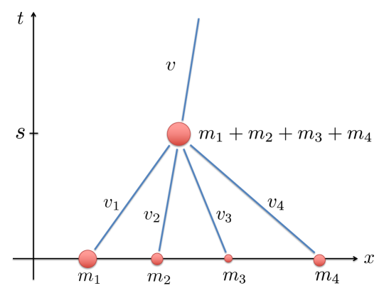
Figure 1: Four point masses which move freely along the real line and undergo a perfectly inelastic collision when they collide at time $s$. The velocity $v$ of the resulting particle satisfies $m_{1}v_{1}+m_{2}v_{2}+m_{3}v_{3}+m_{4}v_{4}=(m_{1}+m_{2}+m_{3}+m_{4})v$. Note that the particles are drawn with different sizes to emphasize that they are not assumed to have equal mass.

The proposition below involves trajectories which track the positions of a collection of point masses as described above.

Proposition 2.1.

Suppose $m_{1},\dots,m_{N}>0$, $x_{1},\dots,x_{N}\in\mathbb{R}$ and $v_{1},\dots,v_{N}\in\mathbb{R}$ are given. There exist piecewise linear paths

$$\gamma_{i}:[0,\infty)\rightarrow\mathbb{R}\quad(i=1,\dots,N)$$

with

$$\gamma_{i}(0)=x_{i}\quad\text{and}\quad\dot{\gamma}_{i}(0+)=v_{i}$$

that satisfy the following properties.

1. If $\gamma_{i}(s)=\gamma_{j}(s)$, then

   $$\gamma_{i}(t)=\gamma_{j}(t)$$ (2.1)

   for $t\geq s$.

2. Whenever

   $$\gamma_{i_{1}}(t)=\dots=\gamma_{i_{k}}(t)\neq\gamma_{i}(t)\;\;\text{for}\;\;i\not\in\{i_{1},\dots,i_{k}\},$$

   then

   $$\dot{\gamma}_{i_{j}}(t+)=\frac{m_{i_{1}}\dot{\gamma}_{i_{1}}(t-)+\dots+m_{i_{k}}\dot{\gamma}_{i_{k}}(t-)}{m_{i_{1}}+\dots+m_{i_{k}}}$$ (2.2)

   for $j=1,\dots,k$.

Proof.

We will argue by induction on $N$. For $N=2$, there are two cases. The first is when $t\mapsto x_{1}+tv_{1}$ and $t\mapsto x_{2}+tv_{2}$ never intersect. In this scenario, we set

$$\gamma_{i}(t)=x_{i}+tv_{i},\quad t\geq 0$$ (2.3)

for $i=1,2$. Otherwise, there is a first time $s\geq 0$ where the paths $t\mapsto x_{i}+tv_{i}$ intersect. In this case, we set

$$\gamma_{i}(t):=\begin{cases}x_{i}+tv_{i},\quad&t\in[0,s]\\ z+(t-s)\left(\displaystyle\frac{m_{1}v_{1}+m_{2}v_{2}}{m_{1}+m_{2}}\right),\quad&t\in[s,\infty)\end{cases}$$

where $z:=x_{1}+sv_{1}=x_{2}+sv_{2}$.

Now suppose the claim holds for some $N\geq 2$ and suppose $m_{1},\dots,m_{N+1}>0$, $x_{1},\dots,x_{N+1}\in\mathbb{R}$ and $v_{1},\dots,v_{N+1}\in\mathbb{R}$ are given. If none of the paths (2.3) intersect, then we define $\gamma_{i}$ by these linear trajectories for $i=1,\dots,N+1$. If there is at least one intersection, let $s\geq 0$ denote the first time that the trajectories (2.3) intersect. Let us also initially assume that a single subcollection of trajectories intersect for the first time at time $s$

$$z:=x_{i_{1}}+sv_{i_{1}}=\dots=x_{i_{k}}+sv_{i_{k}}\neq x_{i}+sv_{i}\;\;\text{for}\;\;i\not\in\{i_{1},\dots,i_{k}\}$$

($k\geq 2$) and set

$$v=\frac{m_{i_{1}}v_{i_{1}}+\dots+m_{i_{k}}v_{i_{k}}}{m_{i_{1}}+\dots+m_{i_{k}}}.$$

Now consider the $N+1-(k-1)$ masses

$$\{m_{i}\}_{i\neq i_{j}}\quad\text{and}\quad m_{i_{1}}+\dots+m_{i_{k}},$$

initial positions

$$\{x_{i}+sv_{i}\}_{i\neq i_{j}}\quad\text{and}\quad z,$$

and initial velocities

$$\{v_{i}\}_{i\neq i_{j}}\quad\text{and}\quad v.$$

By induction, this data gives rise to $N+1-(k-1)$ trajectories $\{\tilde{\gamma}_{i}\}_{i\neq i_{j}}$ and $\tilde{\gamma}$ from $[0,\infty)\rightarrow\mathbb{R}$, respectively, which satisfy the conclusion of this proposition. We then set

$$\gamma_{i}(t)=\begin{cases}x_{i}+tv_{i},\quad&t\in[0,s]\\ \tilde{\gamma}_{i}(t-s),\quad&t\in[s,\infty)\end{cases}$$

for $i\neq i_{j}$ and

$$\gamma_{i_{j}}(t)=\begin{cases}x_{i_{j}}+tv_{i_{j}},\quad&t\in[0,s]\\ \tilde{\gamma}(t-s),\quad&t\in[s,\infty)\end{cases}$$

for $j=1,\dots,k$. It is immediate from construction that this collection of $N+1$ paths satisfies the desired properties. Finally, we note that a similar argument can be made in the case that more than one subcollection of (2.3) intersect for the first time at $s$. We leave the details to the reader. ∎

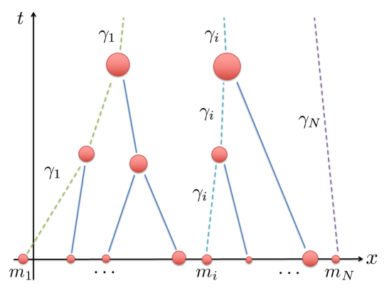
Figure 2: A schematic of the trajectories $\gamma_{1},\dots,\gamma_{N}$ in $\mathbb{R}\times(0,\infty)$ which track the motion of the respective point masses labeled $m_{1},\dots,m_{N}$. The trajectories $\gamma_{1},\gamma_{i}$ and $\gamma_{N}$ are shown with dashed line segments to highlight that they track $m_{1},m_{i}$ and $m_{N}$, respectively.

Any collection of trajectories $\gamma_{1},\dots,\gamma_{N}:[0,\infty)\rightarrow\mathbb{R}$ as specified in the conclusion of Proposition 2.1 are sticky particle trajectories associated with the respective masses $m_{1},\dots,m_{N}$, initial positions $x_{1},\dots,x_{N}\in\mathbb{R}$ and initial velocities $v_{1},\dots,v_{N}$. Moreover, we interpret $\gamma_{i}(t)$ as the location of point mass $m_{i}$ at time $t\geq 0$; this mass could be by itself or a part of a larger mass if it has collided with other particles prior to time $t$. The other two properties in the proposition represent the rules of inelastic collisions: particles stick together and their velocities average when they collide. See Figure 2 for a schematic.

For the remainder of this section, we suppose that masses $m_{1},\dots,m_{N}>0$ satisfy

$$\sum^{N}_{i=1}m_{i}=1,$$

initial positions $x_{1},\dots,x_{N}\in\mathbb{R}$ and initial velocities $v_{1},\dots,v_{N}\in\mathbb{R}$ are given and fixed. We will denote $\gamma_{1},\dots,\gamma_{N}$ as a corresponding collection of sticky particle trajectories and prove various important features of these paths. The first of which is an averaging property.

Proposition 2.2.

Assume $g:\mathbb{R}\rightarrow\mathbb{R}$. Then

$$\sum^{N}_{i=1}m_{i}g(\gamma_{i}(t))\dot{\gamma}_{i}(t+)=\sum^{N}_{i=1}m_{i}g(\gamma_{i}(t))\dot{\gamma}_{i}(s+)$$ (2.4)

for $0\leq s\leq t$.

Proof.

If the none of the trajectories $\gamma_{1},\dots,\gamma_{N}$ intersect, then $\dot{\gamma}_{1},\dots,\dot{\gamma}_{N}$ are each constant and (2.4) trivially holds. Alternatively, some of the trajectories $\gamma_{1},\dots,\gamma_{N}$ intersect and there are at most finitely many times when at least two of them agree for the first time. We will call these times first intersection times and use $0<t_{1}<\dots<t_{\ell}<\infty$ to denote this collection of times. We will also set $t_{0}=0$.

As each $[0,\infty)\ni t\mapsto\dot{\gamma}_{i}(t+)$ is constant on the intervals $[t_{0},t_{1}),[t_{1},t_{2}),\dots$, $[t_{\ell-1},t_{\ell}),[t_{\ell},\infty)$, it suffices to show

$$\sum^{N}_{i=1}m_{i}g(\gamma_{i}(t))\dot{\gamma}_{i}(t_{r}+)=\sum^{N}_{i=1}m_{i}g(\gamma_{i}(t))\dot{\gamma}_{i}(t_{k}+)$$ (2.5)

where $t_{r}$ is the largest of $t_{0},\dots,t_{\ell}$ that is less than $t$ and $k=0,\dots,r$. We will prove (2.5) by induction. For $k=r$, (2.5) is immediate. So we will assume that it holds for some $k\in\{1,\dots,r\}$ and then show how this assumption implies the assertion holds for $k-1$. At time $t_{k}$, let us initially suppose that one sub-collection $\{\gamma_{i_{j}}\}^{n}_{j=1}\subset\{\gamma_{i}\}^{N}_{i=1}$ of paths intersect for the first time. Observe that these trajectories also coincide at time $t$ as $t\geq t_{k}$; we will call this common path $\overline{\gamma}:[t_{k},\infty)\rightarrow\mathbb{R}$. We also note that

$$\dot{\gamma}_{i_{j}}(t_{k}+)=v_{k}:=\frac{m_{i_{1}}\dot{\gamma}_{i_{1}}(t_{k}-)+\dots+m_{i_{n}}\dot{\gamma}_{i_{n}}(t_{k}-)}{m_{i_{1}}+\dots+m_{i_{n}}}\quad$$

for $j=1,\dots,n$ and $\dot{\gamma}_{i}(t_{k}+)=\dot{\gamma}_{i}(t_{k-1}+)$ for $i\neq i_{j}$.

Taking these observations into account and the induction hypothesis, we find

$$\sum^{N}_{i=1}m_{i}g(\gamma_{i}(t))\dot{\gamma}_{i}(t_{r}+) =\sum^{N}_{i=1}m_{i}g(\gamma_{i}(t))\dot{\gamma}_{i}(t_{k}+)$$

$$=\sum_{i\neq i_{j}}m_{i}g(\gamma_{i}(t))\dot{\gamma}_{i}(t_{k}+)+\sum^{n}_{j=1}m_{i_{j}}g(\gamma_{i_{j}}(t))\dot{\gamma}_{i_{j}}(t_{k}+)$$

$$=\sum_{i\neq i_{j}}m_{i}g(\gamma_{i}(t))\dot{\gamma}_{i}(t_{k-1}+)+\left(\sum^{n}_{j=1}m_{i_{j}}\right)g(\overline{\gamma}(t))v_{k}$$

$$=\sum_{i\neq i_{j}}m_{i}g(\gamma_{i}(t))\dot{\gamma}_{i}(t_{k-1}+)+g(\overline{\gamma}(t))\left(\sum^{n}_{j=1}m_{i_{j}}\right)v_{k}$$

$$=\sum_{i\neq i_{j}}m_{i}g(\gamma_{i}(t))\dot{\gamma}_{i}(t_{k-1}+)+g(\overline{\gamma}(t))\sum^{n}_{j=1}m_{i_{j}}\dot{\gamma}_{i_{j}}(t_{k}-)$$

$$=\sum_{i\neq i_{j}}m_{i}g(\gamma_{i}(t))\dot{\gamma}_{i}(t_{k-1}+)+g(\overline{\gamma}(t))\sum^{n}_{j=1}m_{i_{j}}\dot{\gamma}_{i_{j}}(t_{k-1}+)$$

$$=\sum_{i\neq i_{j}}m_{i}g(\gamma_{i}(t))\dot{\gamma}_{i}(t_{k-1}+)+\sum^{n}_{j=1}m_{i_{j}}g(\gamma_{i_{j}}(t))\dot{\gamma}_{i_{j}}(t_{k-1}+)$$

$$=\sum^{N}_{i=1}m_{i}g(\gamma_{i}(t))\dot{\gamma}_{i}(t_{k-1}+).$$

This argument is readily adapted to the case where more than one sub-collection of $\gamma_{1},\dots,\gamma_{N}$ intersect for the first time at $t_{k}$. Therefore, we conclude (2.5) and consequently (2.4). ∎

Using this averaging property, we can derive an elementary inequality involving the velocities $\dot{\gamma}_{i}$ at different times. To this end, we set

$$v(x,t):=\begin{cases}\dot{\gamma}_{i}(t+),\quad&x=\gamma_{i}(t)\\ 0,\quad&\text{otherwise}.\end{cases}$$ (2.6)

In view of Proposition 2.1 part $(i)$, $\dot{\gamma}_{i}(t+)=\dot{\gamma}_{j}(t+)$ if $\gamma_{i}(t)=\gamma_{j}(t)$. As a result, $v:\mathbb{R}\times[0,\infty)\rightarrow\mathbb{R}$ is well defined.

Corollary 2.3.

For $0\leq s\leq t$,

$$\frac{1}{2}\sum^{N}_{i=1}m_{i}\dot{\gamma}_{i}(t+)^{2}\leq\frac{1}{2}\sum^{N}_{i=1}m_{i}\dot{\gamma}_{i}(s+)^{2}.$$ (2.7)

Proof.

Employing (2.6) and (2.4), we find

$$\sum^{N}_{i=1}m_{i}\dot{\gamma}_{i}(t+)^{2} =\sum^{N}_{i=1}m_{i}\dot{\gamma}_{i}(t+)v(\gamma_{i}(t),t)$$

$$=\sum^{N}_{i=1}m_{i}\dot{\gamma}_{i}(s+)v(\gamma_{i}(t),t)$$

$$=\sum^{N}_{i=1}m_{i}\dot{\gamma}_{i}(s+)\dot{\gamma}_{i}(t+)$$

$$\leq\sum^{N}_{i=1}m_{i}\left(\frac{1}{2}\dot{\gamma}_{i}(s+)^{2}+\frac{1}{2}\dot{\gamma}_{i}(t+)^{2}\right)$$

$$=\frac{1}{2}\sum^{N}_{i=1}m_{i}\dot{\gamma}_{i}(s+)^{2}+\frac{1}{2}\sum^{N}_{i=1}m_{i}\dot{\gamma}_{i}(t+)^{2}.$$

∎

The last property we will derive is the quantitative sticky particle property. It follows easily from the next assertion.

Proposition 2.4.

For each $i,j\in\{1,\dots,N\}$ and $t>0$,

$$(\dot{\gamma}_{i}(t+)-\dot{\gamma}_{j}(t+))(\gamma_{i}(t)-\gamma_{j}(t))\leq\frac{1}{t}(\gamma_{i}(t)-\gamma_{j}(t))^{2}.$$ (2.8)

Proof.

Set $t_{0}=0$, and suppose $t_{1}<\dots<t_{\ell}<\infty$ are the possible first intersection times of the trajectories $\gamma_{1},\dots,\gamma_{N}$. We will focus on an interval $(t_{k-1},t_{k})$ where no collisions occur. Between these intersection times, all trajectories are linear so

$$\gamma_{i}(t)=a_{i}+tw_{i}\quad\text{and}\quad\gamma_{i}(t)=a_{j}+tw_{j}$$

for $t\in(t_{k-1},t_{k})$, some $a_{i},a_{j},w_{i},w_{j}\in\mathbb{R}$. Without loss of generality, we will assume that $\gamma_{i}(t)\neq\gamma_{j}(t)$ for $t\in(t_{k-1},t_{k})$.

If

$$(a_{i}-a_{j})(w_{i}-w_{j})<0,$$ (2.9)

then the linear paths $a_{i}+tw_{i}$ and $a_{j}+tw_{j}$ will eventually intersect. By our assumption, $t_{k}$ must be less than or equal to this intersection time. That is,

$$t_{k}\leq-\frac{(a_{i}-a_{j})(w_{i}-w_{j})}{(w_{i}-w_{j})^{2}}.$$

As a result,

$$(\dot{\gamma}_{i}(t)-\dot{\gamma}_{j}(t))(\gamma_{i}(t)-\gamma_{j}(t)) =(w_{i}-w_{j})(a_{i}+tw_{i}-(a_{j}+tw_{j}))$$

$$=(w_{i}-w_{j})(a_{i}-a_{j})+t(w_{i}-w_{j})^{2}$$

$$\leq(w_{i}-w_{j})(a_{i}-a_{j})+t_{k}(w_{i}-w_{j})^{2}$$

$$\leq 0$$

for $t\in(t_{k-1},t_{k})$.

Alternatively, if (2.9) does not hold, then

$$(\dot{\gamma}_{i}(t)-\dot{\gamma}_{j}(t))(\gamma_{i}(t)-\gamma_{j}(t)) =(w_{i}-w_{j})(a_{i}-a_{j})+t(w_{i}-w_{j})^{2}$$

$$\leq 2(w_{i}-w_{j})(a_{i}-a_{j})+t(w_{i}-w_{j})^{2}$$

$$\leq\frac{1}{t}(a_{i}-a_{j})^{2}+2(w_{i}-w_{j})(a_{i}-a_{j})+t(w_{i}-w_{j})^{2}$$

$$=\frac{1}{t}(a_{i}-a_{j}+t(w_{i}-w_{j}))^{2}$$

$$=\frac{1}{t}(a_{i}+tw_{i}-(a_{j}+tw_{j}))^{2}$$

$$=\frac{1}{t}(\gamma_{i}(t)-\gamma_{j}(t))^{2}.$$

Thus (2.8) holds for all $t\in(t_{k-1},t_{k})$. It is also not hard to see the argument above implies that (2.8) holds for $(t_{\ell},\infty)$, as well. Taking limits in (2.8) as $t\searrow t_{k}$ for $k=1,\dots,\ell$, we conclude that it actually holds for all $t>0$. ∎

Corollary 2.5.

For each $i,j\in\{1,\dots,N\}$ and $0<s\leq t<\infty$,

$$\frac{1}{t}|\gamma_{i}(t)-\gamma_{j}(t)|\leq\frac{1}{s}|\gamma_{i}(s)-\gamma_{j}(s)|.$$ (2.10)

Proof.

Observe

$$\frac{d}{dt}\frac{1}{2}(\gamma_{i}(t)-\gamma_{j}(t))^{2} =(\gamma_{i}(t)-\gamma_{j}(t))(\dot{\gamma}_{i}(t)-\dot{\gamma}_{j}(t))$$

$$=(\gamma_{i}(t)-\gamma_{j}(t))(v(\gamma_{i}(t),t)-v(\gamma_{j}(t),t))$$

$$\leq\frac{1}{t}(\gamma_{i}(t)-\gamma_{j}(t))^{2}$$

for almost every $t>0$. As a result,

$$\frac{d}{dt}\frac{1}{t^{2}}(\gamma_{i}(t)-\gamma_{j}(t))^{2} =\frac{1}{t^{2}}\frac{d}{dt}(\gamma_{i}(t)-\gamma_{j}(t))^{2}-\frac{2}{t^{3}}(\gamma_{i}(t)-\gamma_{j}(t))^{2}$$

$$\leq\frac{2}{t^{3}}(\gamma_{i}(t)-\gamma_{j}(t))^{2}-\frac{2}{t^{3}}(\gamma_{i}(t)-\gamma_{j}(t))^{2}$$

$$=0.$$

∎

We can summarize these properties and relate them to Proposition 1.3 as described below.

Proposition 2.6.

Define

$$\eta=\sum^{N}_{i=1}m_{i}\delta_{\gamma_{i}}\in{\cal P}(\Gamma)$$ (2.11)

and $\rho_{0}=\sum^{N}_{i=1}m_{i}\delta_{x_{i}}$, and suppose $v_{0}:\mathbb{R}\rightarrow\mathbb{R}$ satisfies

$$v_{0}(x_{i})=v_{i},\;\;\text{for}\;\;i=1,\dots,N.$$

Then the following assertions hold.

1. $\rho_{0}=e_{0}{{}_{\#}}\eta$.

2. For each $0<s\leq t$ and $\gamma,\xi\in\textup{supp}(\eta)$,

   $$\frac{1}{t}|\gamma(t)-\xi(t)|\leq\frac{1}{s}|\gamma(s)-\xi(s)|.$$ (2.12)

3. For each $\gamma\in\textup{supp}(\eta)$, $\gamma:[0,\infty)\rightarrow\mathbb{R}$ is continuous and piecewise linear.

4. Define $v:\mathbb{R}\times[0,\infty)\rightarrow\mathbb{R}$ via (2.6). For $\gamma\in\textup{supp}(\eta)$,

   $$\dot{\gamma}(t+)=v(\gamma(t),t),\quad t\geq 0.$$ (2.13)

5. For $h:\mathbb{R}\rightarrow\mathbb{R}$ and all but finitely many $t>0$

   $$\int_{\Gamma}\dot{\gamma}(t)h(\gamma(t))d\eta(\gamma)=\int_{\Gamma}v_{0}(\gamma(0))h(\gamma(t))d\eta(\gamma).$$ (2.14)

6. For all $0\leq s\leq t<\infty$,

   $$\int_{\mathbb{R}}\frac{1}{2}\dot{\gamma}(t+)^{2}d\eta(\gamma)\leq\int_{\mathbb{R}}\frac{1}{2}\dot{\gamma}(s+)^{2}d\eta(\gamma).$$

Proof.

For $f\in C_{b}(\mathbb{R})$,

$$\int_{\mathbb{R}}f(x)d\rho_{0}(x)=\sum^{N}_{i=1}m_{i}f(x_{i})=\sum^{N}_{i=1}m_{i}f(\gamma_{i}(0))=\int_{\Gamma}f(\gamma(0))d\eta(\gamma).$$

This proves $(i)$. As $\textup{supp}(\eta)=\{\gamma_{1},\dots,\gamma_{N}\}$, $(ii)$ follows from Corollary 2.5. Part $(iii)$ is due to Proposition 2.1, $(iv)$ is immediate from the definition of (2.6), $(v)$ follows from Proposition 2.2 (with $s=0$), and $(vi)$ is a consequence of Corollary 2.3. ∎

3 Proof of Proposition 1.3

This section is devoted to the proof of Proposition 1.3. To this end, we let $\rho_{0}\in{\cal P}(\mathbb{R})$ and suppose $v_{0}:\mathbb{R}\rightarrow\mathbb{R}$ is continuous with

$$\int_{\mathbb{R}}v_{0}^{2}d\rho_{0}<\infty.$$

By Lemma A.1, there is a sequence $(\rho^{k}_{0})_{k\in\mathbb{N}}$ such that each $\rho^{k}_{0}\in{\cal P}(\mathbb{R})$ is a convex combination of Dirac measures, $\rho^{k}_{0}\rightarrow\rho_{0}$ narrowly, and

$$\lim_{k\rightarrow\infty}\int_{\mathbb{R}}v_{0}^{2}d\rho^{k}_{0}=\int_{\mathbb{R}}v_{0}^{2}d\rho_{0}.$$ (3.1)

We also recall that since $\rho^{k}_{0}\rightarrow\rho_{0}$ narrowly, there is a function $\theta:\mathbb{R}\rightarrow[0,\infty)$ with compact sublevel sets for which

$$\sup_{k\in\mathbb{N}}\int_{\mathbb{R}}\theta d\rho^{k}_{0}<\infty$$ (3.2)

(Remark 5.1.5 of [1]).

As $\rho^{k}_{0}$ is a convex combination of Dirac measures, Proposition 2.6 implies there is $\eta^{k}\in{\cal P}(\Gamma)$ which satisfies:

1. $\rho^{k}_{0}=e_{0}{{}_{\#}}\eta^{k}$.

2. For each $0<s\leq t$ and $\gamma,\xi\in\textup{supp}(\eta^{k})$,

   $$\frac{1}{t}|\gamma(t)-\xi(t)|\leq\frac{1}{s}|\gamma(s)-\xi(s)|.$$ (3.3)

3. For $h:\mathbb{R}\rightarrow\mathbb{R}$ and all but finitely many $t>0$

   $$\int_{\Gamma}\dot{\gamma}(t)h(\gamma(t))d\eta^{k}(\gamma)=\int_{\Gamma}v_{0}(\gamma(0))h(\gamma(t))d\eta^{k}(\gamma).$$ (3.4)

4. For all but finitely many $t\geq 0$,

   $$\int_{\Gamma}\dot{\gamma}(t)^{2}d\eta^{k}(\gamma)\leq\int_{\mathbb{R}}v_{0}^{2}d\rho^{k}_{0}.$$ (3.5)

We will show that $(\eta^{k})_{k\in\mathbb{N}}$ has a convergent subsequence.

Lemma 3.1.

There is a subsequence $(\eta^{k_{j}})_{j\in\mathbb{N}}$ and $\eta^{\infty}\in{\cal P}(\Gamma)$ such that

$$\lim_{j\rightarrow\infty}\int_{\Gamma}{\cal F}(\gamma)d\eta^{k_{j}}(\gamma)=\int_{\Gamma}{\cal F}(\gamma)d\eta^{\infty}(\gamma)$$ (3.6)

for each bounded, continuous ${\cal F}:\Gamma\rightarrow\mathbb{R}$. Moreover,

$$\lim_{R\rightarrow\infty}\int_{|\gamma(t_{2})-\gamma(t_{1})|\geq R}|\gamma(t_{2})-\gamma(t_{1})|d\eta^{k}(\gamma)=0$$ (3.7)

for each $t_{1},t_{2}\geq 0$ and

$$\lim_{R\rightarrow\infty}\int_{|v_{0}(\gamma(0))|\geq R}|v_{0}(\gamma(0))|d\eta^{k}(\gamma)=0$$ (3.8)

uniformly in $k\in\mathbb{N}$.

Proof.

1. First we define

$$X:=\left\{\gamma\in\Gamma\;|\;\gamma:[0,\infty)\rightarrow\mathbb{R}\;\text{absolutely continuous and}\;\int^{n}_{0}\dot{\gamma}(t)^{2}dt<\infty\;\text{for all $n\in\mathbb{N}$}\right\}$$ (3.9)

and set

$$\Phi(\gamma):=\begin{cases}\theta(\gamma(0))+\displaystyle\sum_{n=1}\frac{1}{2^{n}}\int^{n}_{0}\dot{\gamma}(t)^{2}dt,\quad&\gamma\in X\\ +\infty,\quad&\gamma\not\in X.\end{cases}$$ (3.10)

Using (3.5) gives

$$\int_{\Gamma}\Phi(\gamma)d\eta^{k}(\gamma) =\int_{\Gamma}\left[\theta(\gamma(0))+\displaystyle\sum_{n=1}\frac{1}{2^{n}}\int^{n}_{0}\dot{\gamma}(t)^{2}dt\right]d\eta^{k}(\gamma)$$

$$=\int_{\Gamma}\theta(\gamma(0))d\eta^{k}(\gamma)+\sum_{n=1}\frac{1}{2^{n}}\int_{\Gamma}\left(\int^{n}_{0}\dot{\gamma}(t)^{2}dt\right)d\eta^{k}(\gamma)$$

$$=\int_{\mathbb{R}}\theta d\rho^{k}_{0}+\sum_{n=1}\frac{1}{2^{n}}\int^{n}_{0}\left(\int_{\Gamma}\dot{\gamma}(t)^{2}d\eta^{k}(\gamma)\right)dt$$

$$\leq\int_{\mathbb{R}}\theta d\rho^{k}_{0}+\sum_{n=1}\frac{1}{2^{n}}\int^{n}_{0}\left(\int_{\mathbb{R}}v_{0}^{2}d\rho^{k}_{0}\right)dt$$

$$=\int_{\mathbb{R}}\theta d\rho^{k}_{0}+\sum_{n=1}\frac{n}{2^{n}}\int_{\mathbb{R}}v_{0}^{2}d\rho^{k}_{0}$$

$$=\int_{\mathbb{R}}\left(\theta+2v_{0}^{2}\right)\rho^{k}_{0}.$$ (3.11)

In view of (3.1) and (3.2),

$$\sup_{k\in\mathbb{N}}\int_{\Gamma}\Phi(\gamma)d\eta^{k}(\gamma)<\infty.$$

By the Arzelà-Ascoli theorem, the sublevel sets of $\Phi$ are compact within $\Gamma$. Here we recall that $\Gamma$ is a complete, separable metric space when equipped with the distance

$$d(\gamma,\zeta):=\sum_{n\in\mathbb{N}}\frac{1}{2^{n}}\left(\frac{\displaystyle\max_{0\leq t\leq n}|\gamma(t)-\zeta(t)|}{1+\displaystyle\max_{0\leq t\leq n}|\gamma(t)-\zeta(t)|}\right)\quad(\gamma,\xi\in\Gamma)$$

(Proposition A.2 of [8]). As a result, Prokhorov’s theorem (Theorem 5.1.3 in [1]) asserts that $(\eta^{k})_{k\in\mathbb{N}}$ has a narrowly convergent subsequence. That is, there is a subsequence $(\eta^{k_{j}})_{j\in\mathbb{N}}$ and $\eta^{\infty}\in{\cal P}(\Gamma)$ such that (3.6) holds.

2. For $t_{1}\leq t_{2}$,

$$\int_{|\gamma(t_{2})-\gamma(t_{1})|\geq R}|\gamma(t_{2})-\gamma(t_{1})|d\eta^{k}(\gamma) \leq\frac{1}{R}\int_{\Gamma}|\gamma(t_{2})-\gamma(t_{1})|^{2}d\eta^{k}(\gamma)$$

$$\leq\frac{t_{2}-t_{1}}{R}\int_{\Gamma}\left(\int^{t_{2}}_{t_{1}}\dot{\gamma}(t)^{2}dt\right)d\eta^{k}(\gamma)$$

$$=\frac{t_{2}-t_{1}}{R}\int^{t_{2}}_{t_{1}}\left(\int_{\Gamma}\dot{\gamma}(t)^{2}d\eta^{k}(\gamma)\right)dt$$

$$\leq\frac{(t_{2}-t_{1})^{2}}{R}\int_{\mathbb{R}}v_{0}^{2}d\rho_{0}^{k}.$$

Again appealing to (3.1), we conclude that the limit (3.7) is uniform in $k\in\mathbb{N}$. Likewise

$$\int_{|v_{0}(\gamma(0))|\geq R}|v_{0}(\gamma(0))|d\eta^{k}(\gamma)\leq\frac{1}{R}\int_{\Gamma}v_{0}(\gamma(0))^{2}d\eta^{k}(\gamma)=\frac{1}{R}\int_{\mathbb{R}}v_{0}^{2}d\rho^{k}_{0}\rightarrow 0$$

as $R\rightarrow\infty$ uniformly in $k\in\mathbb{N}$. ∎

Proof of Proposition 1.3.

We will now show $\eta^{\infty}$ satisfies conditions $(i)-(vi)$ in the statement of Proposition 1.3.

Proof of $(i)$: As $e_{0}:\Gamma\rightarrow\mathbb{R}$ is continuous, it follows from the narrow convergence of $\eta^{k_{j}}\rightarrow\eta^{\infty}$ in ${\cal P}(\Gamma)$ that

$$\rho_{0}=\lim_{j\rightarrow\infty}e_{0}{{}_{\#}}\eta^{k_{j}}=e_{0}{{}_{\#}}\eta^{\infty}.$$

Proof of $(ii)$: Suppose $\gamma,\xi\in\textup{supp}(\eta^{\infty})$. Then there are sequences $(\gamma^{j})_{j\in\mathbb{N}}$ and $(\xi^{j})_{j\in\mathbb{N}}$ such that $\gamma^{j},\xi^{j}\in\textup{supp}(\eta^{k_{j}})$ for all $j\in\mathbb{N}$ and $\gamma^{j}\rightarrow\gamma$ and $\xi^{j}\rightarrow\xi$ in $\Gamma$ (Lemma 5.1.8 of [1]). Combining with (3.3), we have

$$\frac{1}{t}|\gamma(t)-\xi(t)| =\lim_{j\rightarrow\infty}\frac{1}{t}|\gamma^{j}(t)-\xi^{j}(t)|$$

$$\leq\lim_{j\rightarrow\infty}\frac{1}{s}|\gamma^{j}(s)-\xi^{j}(s)|$$

$$=\frac{1}{t}|\gamma(s)-\xi(s)|$$

for $0<s\leq t$.

Proof of $(iii)$: Recall that $\Phi:\Gamma\rightarrow[0,\infty]$ defined in (3.10) has compact sublevel sets and is thus lower semicontinuous. By narrow convergence and (3),

$$\int_{\Gamma}\Phi(\gamma)d\eta^{\infty}(\gamma)\leq\liminf_{j\rightarrow\infty}\int_{\Gamma}\Phi(\gamma)d\eta^{k_{j}}(\gamma)\leq\liminf_{j\rightarrow\infty}\int_{\mathbb{R}}\left(\theta+2v_{0}^{2}\right)d\rho_{0}^{k_{j}}<\infty.$$ (3.12)

In particular, $\Phi(\gamma)<\infty$ for $\eta^{\infty}$ almost every $\gamma\in\Gamma$. As a result, $\gamma:[0,\infty)\rightarrow\mathbb{R}$ is absolutely continuous for $\eta^{\infty}$ almost every $\gamma\in\Gamma$.

Proof of $(iv)$: For each $(x,t,s)\in\mathbb{R}\times(0,\infty)\times(0,\infty)$ with $s\leq t$, define

$$f(x,t,s):=\inf\left\{\xi(t)+\frac{t}{s}|x-\xi(s)|:\xi\in\text{supp}(\eta^{\infty})\right\}.$$ (3.13)

If $x=\gamma(s)$ with $\gamma\in\text{supp}(\eta^{\infty})$ and $s\leq t$, we can choose $\xi=\gamma$ in the above infimum to get $f(\gamma(s),t,s)\leq\gamma(t)$. By part $(ii)$ of this proof, $\xi(t)+\frac{t}{s}|\gamma(s)-\xi(s)|\geq\gamma(t)$ for all $\xi\in\text{supp}(\eta^{\infty})$. It follows that

$$f(\gamma(s),t,s)=\gamma(t)$$

for $\gamma\in\text{supp}(\eta^{\infty})$ and $s\leq t$.

For $n\in\mathbb{N}$, set

$$v_{n}(x,t):=n(f(x,t+1/n,t)-x)$$ (3.14)

for $(x,t)\in\mathbb{R}\times(0,\infty)$. As $f$ is upper semicontinuous, $v_{n}$ is Borel measurable. Moreover,

$$v_{n}(\gamma(t),t)=n(\gamma(t+1/n)-\gamma(t))$$

for $\gamma\in\text{supp}(\eta^{\infty})$ and $t>0$.

It is routine to verify that

$${\cal D}=\left\{(\gamma,t)\in\Gamma\times(0,\infty):\dot{\gamma}(t)\;\;\text{exists}\right\}$$

is a Borel subset of $\Gamma\times(0,\infty)$. Furthermore,

$$D(\gamma,t)=\begin{cases}\displaystyle\dot{\gamma}(t),\quad&(\gamma,t)\in{\cal D}\\ 0,\quad&\text{otherwise}\end{cases}$$ (3.15)

is Borel measurable as $\dot{\gamma}(t)=\lim_{n\rightarrow\infty}n\left(\gamma(t+1/n)-\gamma(t)\right)$ for $(\gamma,t)\in{\cal D}$. We also set

$$\Upsilon={\cal D}\cap(\text{supp}(\eta^{\infty})\times(0,\infty))$$

and note that the collection of Borel subsets of $\Upsilon$ is

$$\left\{\Upsilon\cap{\cal A}:\;\text{Borel}\;{\cal A}\subset\Gamma\times(0,\infty)\right\}.$$

Observe that for every $(\gamma,t)\in\Upsilon$,

$$D(\gamma,t) =\dot{\gamma}(t)$$

$$=\lim_{n\rightarrow\infty}n\left(\gamma(t+1/n)-\gamma(t)\right)$$

$$=\lim_{n\rightarrow\infty}v_{n}(\gamma(t),t)$$

$$=\lim_{n\rightarrow\infty}v_{n}\circ E(\gamma,t).$$

Here

$$E:\Gamma\times(0,\infty)\rightarrow\mathbb{R}\times(0,\infty);(\gamma,t)\mapsto(\gamma(t),t)$$

is continuous, so

$${\cal G}:=\left\{\Upsilon\cap E^{-1}(B):\;\textup{Borel}\;B\subset\mathbb{R}\times(0,\infty)\right\}$$

is a sub-sigma-algebra of the Borel subsets of $\Upsilon$. In particular, any ${\cal G}$ measurable function on $\Upsilon$ is of the form $g\circ E$ for some Borel $g:\mathbb{R}\times(0,\infty)\rightarrow\mathbb{R}$ (Lemma 1.13 [9]).

Since $D$ restricted to $\Upsilon$ is the pointwise limit of ${\cal G}$ measurable functions, it is ${\cal G}$ measurable (Proposition 2.7 of [6], Lemma 1.10 of [9]). That is,

$$D|_{\Upsilon}=v\circ E$$ (3.16)

for a Borel $v:\mathbb{R}\times(0,\infty)\rightarrow\mathbb{R}$. In particular, for $\gamma\in\text{supp}(\eta^{\infty})\cap\{\Phi<\infty\}$

$$\dot{\gamma}(t)=v(\gamma(t),t)\;\;\text{a.e.}\;t>0.$$ (3.17)

Proof of $(v)$: Suppose $h\in C_{b}(\mathbb{R})$ and set $g(z)=\int^{z}_{0}h(w)dw$. For $t_{1}\leq t_{2}$,

$$\int^{t_{2}}_{t_{1}}\int_{\Gamma}\dot{\gamma}(t)h(\gamma(t))d\eta^{k_{j}}(\gamma)dt =\int_{\Gamma}\left(\int^{t_{2}}_{t_{1}}\frac{d}{dt}g(\gamma(t))dt\right)d\eta^{k_{j}}(\gamma)$$

$$=\int_{\Gamma}\left(g(\gamma(t_{2}))-g(\gamma(t_{1}))\right)d\eta^{k_{j}}(\gamma).$$

Also note that $\gamma\mapsto g(\gamma(t_{2}))-g(\gamma(t_{1}))$ is continuous on $\Gamma$ and

$$|g(\gamma(t_{2}))-g(\gamma(t_{1})|\leq\|h\|_{\infty}|\gamma(t_{2})-\gamma(t_{1})|.$$

The previous lemma asserts that $\gamma\mapsto|\gamma(t_{2})-\gamma(t_{1})|$ is uniformly integrable, so

$$\lim_{j\rightarrow\infty}\int^{t_{2}}_{t_{1}}\int_{\Gamma}\dot{\gamma}(t)h(\gamma(t))d\eta^{k_{j}}(\gamma)dt =\lim_{j\rightarrow\infty}\int_{\Gamma}\left(g(\gamma(t_{2}))-g(\gamma(t_{1}))\right)d\eta^{k_{j}}(\gamma)$$

$$=\int_{\Gamma}\left(g(\gamma(t_{2}))-g(\gamma(t_{1}))\right)d\eta^{\infty}(\gamma)$$

$$=\int^{t_{2}}_{t_{1}}\int_{\Gamma}\dot{\gamma}(t)h(\gamma(t))d\eta^{\infty}(\gamma)dt$$

(Lemma 5.1.7 of [1]).

We also note that

$$\gamma\mapsto\int^{t_{2}}_{t_{1}}v_{0}(\gamma(0))h(\gamma(t))dt$$

is continuous on $\Gamma$ and

$$\left|\int^{t_{2}}_{t_{1}}v_{0}(\gamma(0))h(\gamma(t))dt\right|\leq\|h\|_{\infty}(t_{2}-t_{1})|v_{0}(\gamma(0))|.$$

As $\gamma\mapsto|v_{0}(\gamma(0))|$ is uniformly integrable,

$$\lim_{j\rightarrow\infty}\int^{t_{2}}_{t_{1}}\int_{\Gamma}v_{0}(\gamma(0))h(\gamma(t))d\eta^{k_{j}}(\gamma)dt =\lim_{j\rightarrow\infty}\int_{\Gamma}\left(\int^{t_{2}}_{t_{1}}v_{0}(\gamma(0))h(\gamma(t))dt\right)d\eta^{k_{j}}(\gamma)$$

$$=\int_{\Gamma}\left(\int^{t_{2}}_{t_{1}}v_{0}(\gamma(0))h(\gamma(t))dt\right)d\eta^{\infty}(\gamma)$$

$$=\int^{t_{2}}_{t_{1}}\int_{\Gamma}v_{0}(\gamma(0))h(\gamma(t))d\eta^{\infty}(\gamma)dt.$$

Thus we can integrate (3.4) from $t_{1}$ to $t_{2}$ and send $k=k_{j}\rightarrow\infty$ to conclude

$$\int^{t_{2}}_{t_{1}}\int_{\Gamma}\dot{\gamma}(t)h(\gamma(t))d\eta^{\infty}(\gamma)dt=\int^{t_{2}}_{t_{1}}\int_{\Gamma}v_{0}(\gamma(0))h(\gamma(t))d\eta^{\infty}(\gamma)dt.$$ (3.18)

Since $t_{1},t_{2}$ are arbitrary, this proves part $(v)$.

Proof of $(vi)$: By (3.12),

$$\int^{n}_{0}\left(\int_{\Gamma}\dot{\gamma}(t)^{2}d\eta^{\infty}(\gamma)\right)dt\leq 2^{n}\int_{\Gamma}\Phi(\gamma)d\eta^{\infty}(\gamma)<\infty$$

for all $n\in\mathbb{N}$. As a result,

$$\int_{\Gamma}v(\gamma(t),t)^{2}d\eta^{\infty}(\gamma)=\int_{\Gamma}\dot{\gamma}(t)^{2}d\eta^{\infty}(\gamma)<\infty$$

for almost every $t>0$. We can also use part $(v)$ of this theorem and the function $f$ defined in (3.13) to find

$$\int_{\Gamma}\dot{\gamma}(t)h(\gamma(t))d\eta^{\infty}(\gamma) =\int_{\Gamma}v_{0}(\gamma(0))h(\gamma(t))d\eta^{\infty}(\gamma)$$

$$=\int_{\Gamma}v_{0}(\gamma(0))h(f(\gamma(s),t,s))d\eta^{\infty}(\gamma)$$

$$=\int_{\Gamma}\dot{\gamma}(s)h(f(\gamma(s),t,s))d\eta^{\infty}(\gamma)$$

$$=\int_{\Gamma}\dot{\gamma}(s)h(\gamma(t))d\eta^{\infty}(\gamma)$$

for almost every $t,s\in[0,\infty)$ with $s\leq t$ and $h\in C_{b}(\mathbb{R})$.

By approximation, we also have

$$\int_{\Gamma}\dot{\gamma}(t)h(\gamma(t))d\eta^{\infty}(\gamma)=\int_{\Gamma}\dot{\gamma}(s)h(\gamma(t))d\eta^{\infty}(\gamma)$$ (3.19)

for almost every $t,s\in[0,\infty)$ with $s\leq t$ and each Borel $h:\mathbb{R}\rightarrow\mathbb{R}$ with

$$\int_{\Gamma}h(\gamma(t))^{2}d\eta^{\infty}(\gamma)<\infty.$$

See for instance Theorem 7.9 in [6]. Consequently,

$$\int_{\Gamma}\dot{\gamma}(t)^{2}d\eta^{\infty}(\gamma) =\int_{\Gamma}\dot{\gamma}(t)v(\gamma(t),t)d\eta^{\infty}(\gamma)$$

$$=\int_{\Gamma}\dot{\gamma}(s)v(\gamma(t),t)d\eta^{\infty}(\gamma)$$

$$=\int_{\Gamma}\dot{\gamma}(s)\dot{\gamma}(t)d\eta^{\infty}(\gamma)$$

$$\leq\frac{1}{2}\int_{\Gamma}\dot{\gamma}(s)^{2}d\eta^{\infty}(\gamma)+\frac{1}{2}\int_{\Gamma}\dot{\gamma}(t)^{2}d\eta^{\infty}(\gamma)$$

for almost every $s\leq t$. ∎

4 Solution of the SPS

We will now show how to use a measure $\eta\in{\cal P}(\Gamma)$ from Proposition 1.3 to generate a solution of the SPS for given initial conditions.

Proof of Theorem 1.4.

Let $\eta^{\infty}\in{\cal P}(\Gamma)$ be the probability measure we constructed in our proof of Proposition 1.3. Recall that $\eta^{\infty}$ fulfills conditions $(i)-(vi)$ in the statement of Proposition 1.3, which we will refer to as $(i)-(vi)$ throughout this proof. We set

$$\rho:(0,\infty)\rightarrow{\cal P}(\mathbb{R});t\mapsto e_{t}{{}_{\#}}\eta^{\infty}$$

and proceed to show that $\rho$ and the function $v:\mathbb{R}\times(0,\infty)\rightarrow\mathbb{R}$ from part $(iv)$ is the desired weak solution pair.

1. Let $\psi\in C^{\infty}_{c}(\mathbb{R}\times[0,\infty))$. In view of conditions $(i)$, $(iii)$ and $(iv)$,

$$\int^{\infty}_{0}\int_{\mathbb{R}}(\partial_{t}\psi+v\partial_{x}\psi)d\rho_{t}dt =\int^{\infty}_{0}\int_{\Gamma}(\partial_{t}\psi(\gamma(t),t)+v(\gamma(t),t)\partial_{x}\psi(\gamma(t),t))d\eta^{\infty}(\gamma)dt$$

$$=\int^{\infty}_{0}\int_{\Gamma}(\partial_{t}\psi(\gamma(t),t)+\dot{\gamma}(t)\partial_{x}\psi(\gamma(t),t))d\eta^{\infty}(\gamma)dt$$

$$=\int_{\Gamma}\int^{\infty}_{0}\frac{d}{dt}\psi(\gamma(t),t)dtd\eta^{\infty}(\gamma)$$

$$=-\int_{\Gamma}\psi(\gamma(0),0)d\eta^{\infty}(\gamma)$$

$$=-\int_{\mathbb{R}}\psi(\cdot,0)d\rho_{0}.$$

We also have by condition $(v)$,

$$\int^{\infty}_{0}\int_{\mathbb{R}}(v\partial_{t}\psi+v^{2}\partial_{x}\psi)d\rho_{t}dt =\int^{\infty}_{0}\int_{\Gamma}\dot{\gamma}(t)(\partial_{t}\psi(\gamma(t),t)+v(\gamma(t),t)\partial_{x}\psi(\gamma(t),t))d\eta^{\infty}(\gamma)dt$$

$$=\int^{\infty}_{0}\int_{\Gamma}v_{0}(\gamma(0))(\partial_{t}\psi(\gamma(t),t)+v(\gamma(t),t)\partial_{x}\psi(\gamma(t),t))d\eta^{\infty}(\gamma)dt$$

$$=\int^{\infty}_{0}\int_{\Gamma}v_{0}(\gamma(0))(\partial_{t}\psi(\gamma(t),t)+\dot{\gamma}(t)\partial_{x}\psi(\gamma(t),t))d\eta^{\infty}(\gamma)dt$$

$$=\int^{\infty}_{0}\int_{\Gamma}v_{0}(\gamma(0))\frac{d}{dt}\psi(\gamma(t),t)d\eta^{\infty}(\gamma)dt$$

$$=\int_{\Gamma}v_{0}(\gamma(0))\left(\int^{\infty}_{0}\frac{d}{dt}\psi(\gamma(t),t)dt\right)d\eta^{\infty}(\gamma)$$

$$=-\int_{\Gamma}v_{0}(\gamma(0))\psi(\gamma(0),0)d\eta^{\infty}(\gamma)$$

$$=-\int_{\mathbb{R}}v_{0}\psi(\cdot,0)d\rho_{0}.$$

Consequently, $\rho$ and $v$ is a weak solution pair which satisfies $\rho|_{t=0}=\rho_{0}$ and $v|_{t=0}=v_{0}$.

2. By part $(ii)$ and (3.17),

$$\frac{d}{dt}\frac{(\gamma(t)-\xi(t))^{2}}{t^{2}}=\frac{2}{t^{2}}\left((v(\gamma(t),t)-v(\xi(t),t))(\gamma(t)-\xi(t))-\frac{1}{t}(\gamma(t)-\xi(t))^{2}\right)\leq 0$$ (4.1)

for each $\gamma,\xi\in\text{supp}(\eta^{\infty})\cap\{\Phi<\infty\}$ and almost every $t>0$. Here $\Phi$ was specified in (3.10), and we recall that

$$\eta^{\infty}(\{\Phi<\infty\})=1,$$

which followed from (3.12).

We also note

$$e_{t}(\{\Phi<\infty\}\cap\text{supp}(\eta^{\infty}))=\bigcup_{m\in\mathbb{N}}\{\gamma(t)\in\mathbb{R}:\gamma\in\text{supp}(\eta^{\infty}),\;\Phi(\gamma)\leq m\}$$

is a Borel subset of $\mathbb{R}$ since $\{\gamma(t)\in\mathbb{R}:\gamma\in\text{supp}(\eta^{\infty}),\;\Phi(\gamma)\leq m\}$ is compact for each $m\in\mathbb{N}$. Moreover,

$$\rho_{t}(e_{t}(\{\Phi<\infty\}\cap\text{supp}(\eta^{\infty}))) =\eta^{\infty}\left(e_{t}^{-1}\left(e_{t}(\{\Phi<\infty\}\cap\text{supp}(\eta^{\infty}))\right)\right)$$

$$\geq\eta^{\infty}\left(\{\Phi<\infty\}\cap\text{supp}(\eta^{\infty})\right)$$

$$=1.$$

In view of (4.1),

$$(v(x,t)-v(y,t))(x-y)\leq\frac{1}{t}(x-y)^{2}$$ (4.2)

holds for almost every $t>0$ and for $\rho_{t}$ almost every $x,y\in\mathbb{R}$.

3. By $(iv)$ and $(v)$,

$$\int_{\mathbb{R}}v(x,t)^{2}d\rho_{t}(x)=\int_{\Gamma}\dot{\gamma}(t)^{2}d\eta^{\infty}(\gamma)\leq\int_{\Gamma}v_{0}(\gamma(0))^{2}d\eta^{\infty}(\gamma)=\int_{\mathbb{R}}v_{0}^{2}d\rho_{0}<\infty$$

for almost every $t>0$. Employing part $(vi)$, we also find

$$\int_{\mathbb{R}}\frac{1}{2}v(x,t)^{2}d\rho_{t}(x) =\int_{\Gamma}\frac{1}{2}v(\gamma(t),t)^{2}d\eta^{\infty}(\gamma)$$

$$=\int_{\Gamma}\frac{1}{2}\dot{\gamma}(t)^{2}d\eta^{\infty}(\gamma)$$

$$\leq\int_{\Gamma}\frac{1}{2}\dot{\gamma}(s)^{2}d\eta^{\infty}(\gamma)$$

$$=\int_{\mathbb{R}}\frac{1}{2}v(x,s)^{2}d\rho_{s}(x)$$

for almost every $0<s\leq t$. ∎

Appendix A Approximation lemma

This is a variation of a standard method used to show that ${\cal P}(\mathbb{R})$ is separable. See for the instance Proposition 4.4 of the notes by Onno [14]. The main point is the function $g$ is not assumed to be bounded.

Lemma A.1.

Suppose $\mu\in{\cal P}(\mathbb{R})$ and $g:\mathbb{R}\rightarrow[0,\infty)$ is continuous with

$$\int_{\mathbb{R}}g(x)d\mu(x)<\infty.$$

There is a sequence $(\mu^{k})_{k\in\mathbb{N}}$ for which each $\mu^{k}\in{\cal P}(\mathbb{R})$ is a convex combination of Dirac measures, $\mu^{k}\rightarrow\mu$ narrowly and

$$\int_{\mathbb{R}}g(x)d\mu(x)=\lim_{k\rightarrow\infty}\int_{\mathbb{R}}g(x)d\mu^{k}(x).$$ (A.1)

Proof.

1. Fix $\epsilon\in(0,1)$ and choose $R>0$ so large that

$$\int_{\mathbb{R}\setminus[-R,R)}(1+g(x))d\mu(x)\leq\epsilon.$$ (A.2)

As $g|_{[-R,R]}$ is uniformly continuous, there is $\delta\in(0,\epsilon)$ such that

$$|g(x)-g(y)|\leq\epsilon$$

provided $x,y\in[-R,R]$ and $|x-y|\leq\delta.$ Let us also select a natural number $N$ for which

$$\frac{2R}{N}\leq\delta.$$

In addition, we set

$$y_{j}:=-R+j\left(\frac{2R}{N}\right)\quad j=0,\dots,N$$

and choose any $x_{j}\in[y_{j-1},y_{j})$ for $j=1,\dots,N$. Moreover, we may select $z\not\in[-R,R)$ such that

$$\inf_{\mathbb{R}\setminus[-R,R)}g\geq g(z)-\epsilon.$$

Now define

$$m_{j}:=\mu([y_{j-1},y_{j}))\quad j=0,\dots,N$$

and

$$m:=\sum_{j=1}m_{j}=\mu([-R,R)).$$

Finally, we set

$$\nu:=\sum^{N}_{j=1}m_{j}\delta_{x_{j}}+(1-m)\delta_{z}$$

and note $\nu\in{\cal P}(\mathbb{R})$ is a convex combination of Dirac measures.

2. Suppose $f:\mathbb{R}\rightarrow\mathbb{R}$ satisfies $|f(x)|\leq 1$ and $|f(x)-f(y)|\leq|x-y|$ for each $x,y\in\mathbb{R}$. As $f$ is continuous, there are $z_{j}\in[y_{j-1},y_{j})$ with

$$f(z_{j})m_{j}=\int_{[y_{j-1},y_{j})}f(x)d\mu(x)$$

for $j=1,\dots,N$. Observe

$$\left|\int_{\mathbb{R}}fd\nu-\int_{\mathbb{R}}fd\mu\right| =\left|\sum^{N}_{j=1}m_{j}f(x_{j})+(1-m)f(z)-\int_{\mathbb{R}\setminus[-R,R)}fd\mu-\int_{[-R,R)}fd\mu\right|$$

$$\leq\left|\sum^{N}_{j=1}m_{j}f(x_{j})-\int_{[-R,R)}fd\mu\right|+(1-m)|f(z)|+\int_{\mathbb{R}\setminus[-R,R)}|f|d\mu$$

$$\leq\left|\sum^{N}_{j=1}\left(m_{j}f(x_{j})-\int_{[y_{j-1},y_{j})}fd\mu\right)\right|+(1-m)+\mu(\mathbb{R}\setminus[-R,R))$$

$$\leq\sum^{N}_{j=1}m_{j}|f(x_{j})-f(z_{j})|+2\mu(\mathbb{R}\setminus[-R,R))$$

$$\leq\sum^{N}_{j=1}m_{j}|x_{j}-z_{j}|+2\epsilon$$

$$\leq\sum^{N}_{j=1}m_{j}\delta+2\epsilon$$

$$\leq 3\epsilon.$$

3. We may also choose $w_{j}\in[y_{j-1},y_{j})$ such that

$$g(w_{j})m_{j}=\int_{[y_{j-1},y_{j})}g(x)d\mu(x)$$

for $j=1,\dots,N$. Doing so gives

$$\left|\int_{\mathbb{R}}gd\nu-\int_{\mathbb{R}}gd\mu\right| =\left|\sum^{N}_{j=1}m_{j}g(x_{j})+(1-m)g(z)-\int_{\mathbb{R}\setminus[-R,R)}gd\mu-\int_{[-R,R)}gd\mu\right|$$

$$=\left|\sum^{N}_{j=1}\left(m_{j}g(x_{j})-\int_{[y_{j-1},y_{j})}gd\mu\right)+(1-m)g(z)-\int_{\mathbb{R}\setminus[-R,R)}gd\mu\right|$$

$$\leq\sum^{N}_{j=1}m_{j}|g(x_{j})-g(w_{j})|+\left|\mu(\mathbb{R}\setminus[-R,R))g(z)-\int_{\mathbb{R}\setminus[-R,R)}gd\mu\right|$$

$$\leq\sum^{N}_{j=1}m_{j}\cdot\epsilon+\left|\mu(\mathbb{R}\setminus[-R,R))g(z)-\int_{\mathbb{R}\setminus[-R,R)}gd\mu\right|$$

$$\leq\epsilon+\left|\mu(\mathbb{R}\setminus[-R,R))g(z)-\int_{\mathbb{R}\setminus[-R,R)}gd\mu\right|.$$

As $g\geq 0$ and by our assumption (A.2),

$$\mu(\mathbb{R}\setminus[-R,R))g(z)-\int_{\mathbb{R}\setminus[-R,R)}gd\mu\geq-\epsilon.$$

And by our choice of $z$,

$$\mu(\mathbb{R}\setminus[-R,R))g(z)-\int_{\mathbb{R}\setminus[-R,R)}gd\mu \leq\mu(\mathbb{R}\setminus[-R,R))\left(\inf_{\mathbb{R}\setminus[-R,R)}g+\epsilon\right)-\int_{\mathbb{R}\setminus[-R,R)}gd\mu$$

$$\leq\mu(\mathbb{R}\setminus[-R,R))\inf_{\mathbb{R}\setminus[-R,R)}g-\int_{\mathbb{R}\setminus[-R,R)}gd\mu+\epsilon^{2}$$

$$\leq\epsilon^{2}$$

$$\leq\epsilon.$$

Thus,

$$\left|\int_{\mathbb{R}}gd\nu-\int_{\mathbb{R}}gd\mu\right|\leq 2\epsilon.$$

4. For each $k\in\mathbb{N}$, we can then find $\nu=\mu^{k}\in{\cal P}(\mathbb{R})$ which is a convex combination of Dirac measures and

$$\left|\int_{\mathbb{R}}fd\mu^{k}-\int_{\mathbb{R}}fd\mu\right|\leq\frac{1}{k}$$

for each $k\in\mathbb{N}$ and $f:\mathbb{R}\rightarrow\mathbb{R}$ with $|f(x)|\leq 1$ and $|f(x)-f(y)|\leq|x-y|$ for $x,y\in\mathbb{R}$. It is well known that this type of convergence implies that $\mu^{k}\rightarrow\mu$ narrowly (Remark 5.1.1 in [1]). Since each $\mu^{k}$ can be chosen so that

$$\left|\int_{\mathbb{R}}gd\mu^{k}-\int_{\mathbb{R}}gd\mu\right|\leq\frac{1}{k}\quad(k\in\mathbb{N}),$$

we conclude (A.1), as well. ∎

References

- [1] Luigi Ambrosio, Nicola Gigli, and Giuseppe Savaré. Gradient flows in metric spaces and in the space of probability measures. Lectures in Mathematics ETH Zürich. Birkhäuser Verlag, Basel, second edition, 2008.
- [2] Yann Brenier and Emmanuel Grenier. Sticky particles and scalar conservation laws. SIAM J. Numer. Anal., 35(6):2317–2328, 1998.
- [3] Fabio Cavalletti, Marc Sedjro, and Michael Westdickenberg. A simple proof of global existence for the 1D pressureless gas dynamics equations. SIAM J. Math. Anal., 47(1):66–79, 2015.
- [4] Azzouz Dermoune. Probabilistic interpretation of sticky particle model. Ann. Probab., 27(3):1357–1367, 1999.
- [5] Weinan E, Yu. G. Rykov, and Ya. G. Sinai. Generalized variational principles, global weak solutions and behavior with random initial data for systems of conservation laws arising in adhesion particle dynamics. Comm. Math. Phys., 177(2):349–380, 1996.
- [6] Gerald B. Folland. Real analysis. Pure and Applied Mathematics (New York). John Wiley & Sons, Inc., New York, second edition, 1999. Modern techniques and their applications, A Wiley-Interscience Publication.
- [7] Feimin Huang and Zhen Wang. Well posedness for pressureless flow. Comm. Math. Phys., 222(1):117–146, 2001.
- [8] Ryan Hynd and Hwa Kil Kim. Infinite horizon value functions in the Wasserstein spaces. J. Differential Equations, 258(6):1933–1966, 2015.
- [9] Olav Kallenberg. Foundations of modern probability. Probability and its Applications (New York). Springer-Verlag, New York, second edition, 2002.
- [10] Octave Moutsinga. Convex hulls, sticky particle dynamics and pressure-less gas system. Ann. Math. Blaise Pascal, 15(1):57–80, 2008.
- [11] Luca Natile and Giuseppe Savaré. A Wasserstein approach to the one-dimensional sticky particle system. SIAM J. Math. Anal., 41(4):1340–1365, 2009.
- [12] Truyen Nguyen and Adrian Tudorascu. Pressureless Euler/Euler-Poisson systems via adhesion dynamics and scalar conservation laws. SIAM J. Math. Anal., 40(2):754–775, 2008.
- [13] Truyen Nguyen and Adrian Tudorascu. One-dimensional pressureless gas systems with/without viscosity. Comm. Partial Differential Equations, 40(9):1619–1665, 2015.
- [14] Onno van Gaans. Probability measures on metric spaces, 2019 (accessed September 14, 2019). www.math.leidenuniv.nl/~vangaans/jancol1.pdf.
- [15] Yakov B. Zel’dovich. Gravitational instability: An Approximate theory for large density perturbations. Astron. Astrophys., 5:84–89, 1970.