Dynamo Effect and Turbulence in Hydrodynamic Weyl Metals

Abstract

The dynamo effect is a class of macroscopic phenomena responsible for generation and maintaining magnetic fields in astrophysical bodies. It hinges on hydrodynamic three-dimensional motion of conducting gases and plasmas that achieve high hydrodynamic and/or magnetic Reynolds numbers due to large length scales involved. The existing laboratory experiments modeling dynamos are challenging and involve large apparatuses containing conducting fluids subject to fast helical flows. Here we propose that electronic solid-state materials – in particular, hydrodynamic metals – may serve as an alternative platform to observe some aspects of the dynamo effect. Motivated by recent experimental developments, this paper focuses on hydrodynamic Weyl semimetals, where the dominant scattering mechanism is due to interactions. We derive Navier-Stokes equations along with equations of magneto-hydrodynamics that describe transport of Weyl electron-hole plasma appropriate in this regime. We estimate the hydrodynamic and magnetic Reynolds numbers for this system. The latter is a key figure of merit of the dynamo mechanism. We show that it can be relatively large to enable observation of the dynamo-induced magnetic field bootstrap in experiment. Finally, we generalize the simplest dynamo instability model – Ponomarenko dynamo – to the case of a hydrodynamic Weyl semimetal and show that the chiral anomaly term reduces the threshold magnetic Reynolds number for the dynamo instability.

The dynamo effect is a beautiful astrophysical phenomenon, first proposed by Larmor in 1919 Larmor (1919), that is believed to be responsible for generating and sustaining magnetic fields in galaxies, stars and planets including the Sun and the Earth Ruzmaikin et al. . There exist a large variety of different dynamo mechanisms Gilbert (a, b); Ruzmaikin et al. that all share the same key ingredient – hydrodynamic motion of an electrically conducting gas, fluid or plasma. The dynamo theory deals with the hydrodynamic motion of a conductive medium focussing on the possibility of self-generating and self-sustaining magnetic fields, whose presence has been observed in astrophysical bodies.

As detailed below, the underlying equations of the theory are the Navier-Stokes equations, describing the hydrodynamic motion of the medium, coupled to the Maxwell equations of electromagnetism. In the non-relativistic limit, they give rise to equations of magneto-hydrodynamics (MHD). These are complicated non-linear equations, and their exact solutions represent a great challenge. However, both the solutions of simplified MHD models [e.g., kinematic dynamos, with predetermined velocity fields ${\bf u}({\bf r},t)$] and qualitative arguments Ruzmaikin et al. suggest that the dynamo action is possible when the terms enhancing the magnetic field [e.g. the induction term, ${\bm{\nabla}}\times({\bf u}\times{\bf B})$] overwhelm the magnetic diffusion term, $\eta_{m}\Delta{\bf B}$ (where $\eta_{m}=c^{2}/4\pi\sigma$ where $c$ is the speed of light and $\sigma$ is the conductivity of the medium), which tend to suppress the self-generation. The respective figure of merit is the magnetic Reynolds number Landau and Lifshitz

$$R_{m}=\frac{uL}{\eta_{m}}=uL\frac{4\pi\sigma}{c^{2}},$$ (1)

where $L$ is the characteristic system size and $u$ is the typical velocity of the medium. The threshold value for a dynamo action to commence (usually lying in in the range $R_{m}^{\rm(cr)}\sim 10-100$, with $R_{m}^{\rm(cr)}\approx 17.7$ for the simplest Ponomarenko dynamo Ponomarenko discussed below) depends on system’s geometry and is rarely known exactly. It is clear, however, that the larger $R_{m}$, the more likely and more effective the dynamo action. The conductivity of astrophysical media vary greatly from $10^{-11}{\rm Sm}^{-1}$ for interstellar plasma to $10^{3}{\rm Sm}^{-1}$ for the solar convection shell and $10^{5}{\rm Sm}^{-1}$ for the Earth’s core, but in all of these cases the large magnetic diffusion coefficient is compensated by literally astronomical distances resulting in large magnetic Reynolds numbers, however small the conductivities are. By contrast, laboratory dynamo experiments Lathrop and Forest deal naturally limited system size and use the conductivity and the flow velocities as the only potentially tunable parameters.

Apart from large magnetic Reynolds numbers $R_{m}\gg 1$, the emergence of a dynamo requires a number of other conditions that need to be met. In particular, certain “no-go theorems” Jones have to be overcome, such as the impossibility of a two-dimensional dynamo effect or that in a planar three-dimensional flow (i.e., with one vanishing component of velocity). Finally, it is known the dynamo action is greatly helped by the helicity flow, which may arise either due to the geometry of an imposed flow or due to turbulence. The latter is possible if the second figure of merit, the hydrodynamic Reynolds number

$$R=\frac{uL}{\nu},$$ (2)

where $\nu$ is the kinematic viscosity. Separating both the velocity and magnetic field into a mean-field and fluctuating component - ${\bm{u}}=\overline{\bm{u}}+\delta{\bm{u}}$ and ${\bm{B}}=\overline{\bm{B}}+\delta{\bm{B}}$, and averaging over the small-scale fluctuations results in the Krause-Rädler equations Krause and Rädler ; Parker of mean-field MHD, which in the simplest case of isotropic turbulence is given by

$$\frac{\partial\overline{\bf B}}{\partial t}={\bm{\nabla}}\times(\overline{\bm{u}}\times\overline{\bf B})+{\bm{\nabla}}\times(\alpha\overline{\bf B})+\xi\Delta\overline{\bf B},$$ (3)

where the second term in the right-hand-side is the “new” helicity term allowed in turbulent MHD ($\alpha$-effect). If the velocity field is stationary, Eq. (3) or a similar MHD equation without helicity for non-turbulent flows becomes an eigenvalue problem for the magnetic field growth ${\bf B}({\bf r},t)\propto{\bf B}({\bf r})e^{\gamma t}$. The existence of exponentially growing components (${\rm Re}\,\gamma>0$) indicates an instability towards a self-generating magnetic field (were the imaginary part ${\rm Im}\,\gamma>0$ leads to the field oscillations, which have been suggested Galitski and Sokoloff, by one of the authors to lead, e.g., to periodic cycles of solar magnetic activity).

Apart from the astrophysical context, there has been a tremendous interest in testing the predictions of dynamo theory and modeling a planetary-like or solar-like dynamo action in the laboratory Lathrop and Forest ; Gailitis et al. (2000); Spence et al. (2007); Monchaux et al. (2007). Several impressive laboratory experiments have been carried out and are currently under way that involve setting in motion a liquid metal – sodium or gallium – with the goal to achieve large Reynolds numbers to enable the dynamo mechanism. As obvious from Eqs. (1) and (2), this leads to the challenge of ultra-fast mechanical stirring or rotating the liquid metal.

Here we propose that electronic solid-state systems may provide an alternative platform for observing magnetohydrodynamic effects. Firstly, we list several necessary conditions of the dynamo effect in an electronic system: (i) Transport in the electron liquid should be governed by hydrodynamics, i.e. the primary momentum relaxation mechanism should be electron-electron collisions rather than impurity scattering. (ii) The system and the flow must be essentially three-dimensional. (iii) Large magnetic $R_{m}\gg 1$ and/or hydrodynamic $R\gg 1$ Reynolds numbers are required.

Hydrodynamic transport in solid state [condition (i)] has been a subject of intense recent studies Andreev et al. ; Lucas and Hartnoll ; Lucas and Das Sarma ; Song et al. ; Hartnoll et al. , both theoretical and experimental. On the experimental side, two widely studied platforms for hydrodynamic phenomena are graphene Kumar et al. and Weyl semimetals (WSMs) Gooth et al. (2017, ); Fu et al. . Graphene, however, violates a “no-go dynamo theorem” - condition (ii) requiring 3D flows - and is thus of no relevance to the dynamo effect.

In what follows, we focus on undoped or weakly doped Weyl semimetals. We note that in systems with the power-law quasiparticle dispersion $\epsilon({\bf p})\propto\left|{\bf p}\right|^{\beta}$ with $\beta\leqslant 1$ the creation of electron-hole pairs is suppressed Foster and Aleiner , because the energy and momentum conservation laws cannot be satisfied simultaneously for lowest-order processes. Weyl systems ($\beta=1$) may, therefore, often be considered as electron-hole plasma with a linear particle dispersion.

A WSM generically has an even number of nodes, according to the fermion-doubling theorem Nielsen and Ninomiya (1981), and electrons and holes near different nodes often behave as independent liquids. However, simultaneous application of external electric ${\bf E}$ and magnetic ${\bf B}$ fields results in the quasiparticle transfer from one node to another (chiral anomalyAdler (1969); Bell and Jackiw (1969); Son and Spivak (2013); Burkov (2018, 2014)). For simplicity, we assume in this paper that (a) the system has only two nodes, labeled by $L$ and $R$, with the same quasiparticle dispersion, (b) the entire system is being kept at a constant temperature $T$ and (c) the intranodal equilibration processes are significantly faster than the internodal particle-transfer processes. This allows one to define the chemical potentials $\mu_{\alpha}$ near each node $\alpha=L,R$ and the hydrodynamic velocity ${\bf u}$ of the Weyl fluid. The distribution function of the linearly-dispersing quasiparticless near each node in the absence of electromagnetic fields is given by Narozhny et al. (2017) $f_{\alpha}({\bf k})=\left\{\exp\left[\gamma({\bf u})\left(\pm v_{F}|{\bf k}|-\mu_{\alpha}-{\bf u}\cdot{\bf k}\right)/T\right]+1\right\}^{-1}$, where “+” and “-” refer, respectively, to the conduction and valence bands, and $\gamma({\bf u})=\left(1-u^{2}/v_{F}^{2}\right)^{\frac{1}{2}}$.

The dynamics of charge densities $\rho_{\alpha}$ near node $\alpha$, where $\alpha=L,R$, are described by the continuity equations

$$\partial_{t}\rho_{\alpha}+{\bm{\nabla}\cdot{\bf j}_{\alpha}}-\chi_{\alpha}\frac{ge^{3}}{4\pi^{2}\hbar^{2}c}{\bf E}\cdot{\bf B}+\frac{\rho_{\alpha}-\rho_{\bar{\alpha}}}{\tau_{in}}=0,$$ (4)

where $\chi_{L}=-1$ and $\chi_{R}=+1$ are the “chiralities” of quasiparticles near nodes $L$ and $R$ and $g$ accounts for spin and possibly additional valley degeneracy; $\bar{\alpha}$ labels the node other than $\alpha$; hereinafter $e=-|e|$. The first two terms in Eq. (4) match the usual continuity equation for a liquid with density $\rho_{\alpha}$; the third term ($\propto{\bf E}\cdot{\bf B}$) accounts Burkov (2018, 2014) for the change of the electron concentration at node $\alpha$ due to the chiral anomaly; and the last term in Eq. (4) describes internodal scattering, e.g., due to short-range-correlated quenched disorder, with the internodal scattering time $\tau_{in}$. The electric currents ${\bf j}_{L,R}$ of the charge carriers near the two nodes are given by

$${\bf j}_{\alpha}=\sum_{\beta}\sigma_{\alpha\beta}\left[{\bf E}+\frac{1}{c}{\bf u}\times{\bf B}-\frac{1}{e}{\bm{\nabla}}\mu_{\beta}\right]-\chi_{\alpha}\frac{ge^{2}}{4\pi^{2}\hbar^{2}c}{\bf B}\mu_{\alpha},$$ (5)

where $\alpha,\beta=L,R$; $\mu_{\alpha}$ is the chemical potential near node $\alpha$, and ${\bf u}$ is the hydrodynamic velocity of the Weyl fluid. In this paper we assume that the imbalance of the chemical potentials between the nodes, if any, is small $|\mu_{L}-\mu_{R}|\ll|\mu_{L,R}|,T$. The diagonal components $\sigma_{LL}=\sigma_{RR}$ of the conductivity tensor $\sigma_{\alpha\beta}$ describe the response of charge carriers near each node to the electromagnetic field; the off-diagonal entries $\sigma_{LR}=\sigma_{RL}$ account for the drag of the quasiparticles near each node by the current near the other node. The last term in Eq. (5) describes the chiral magnetic effect Fukushima et al. (2008); Kharzeev et al. (2013), the generation of the charge current by an external magnetic field in the system in the presence of chirality imbalance, $\mu_{L}-\mu_{R}\neq 0$.

Equations (4)-(5), together with the relations Rodionov and Syzranov (2015)

$$\rho_{R,L}=ge\frac{\mu_{R,L}^{3}+\pi^{2}\mu_{R,L}T^{2}}{6\pi^{2}v_{F}^{3}\hbar^{3}}$$ (6)

for the charge density at node $\alpha$ and with Maxwell equations, which involve the total charge density $\rho=\rho_{L}+\rho_{R}$ and the current ${\bf j}={\bf j}_{L}+{\bf j}_{R}$, constitute a closed system of equations which describes charge and current dynamics of the electron liquid in a WSM which moves with velocity ${\bf u}$ in an external electromagnetic field. The motion of such a liquid may be generated by the electromagnetic field, the temperature and chemical potential gradients, or even fast mechanical rotation of the sample.

To determine self-consistently the velocity field ${\bf u}$ (which in practice is a tremendously difficult problem), the system of Eqs. (4)-(6) has to be complemented by the Navier-Stokes equation (derived in Supplemental Material sup (2018))

$$\frac{w_{\alpha}}{v_{F}^{2}}\left(\frac{\partial}{\partial t}+{\bf u}\cdot{\bm{\nabla}}\right){\bf u}=-{\bm{\nabla}}P_{\alpha}-\frac{{\bf u}}{v_{F}^{2}}\frac{\partial P_{\alpha}}{\partial t}+\rho_{\alpha}{\bf E}+\frac{1}{c}\,{\bf j}_{\alpha}\times{\bf B}$$

$$+\frac{{\bf u}}{3}\left(\frac{\partial\varepsilon}{\partial\rho}\right)_{\alpha}\left(\chi_{\alpha}\frac{ge^{3}}{h^{2}c}{\bf E}\cdot{\bf B}-\frac{\rho_{\alpha}-{\rho}_{\bar{\alpha}}}{\tau_{\text{in}}}\right)+\eta{\bm{\nabla}}^{2}{\bf u}+\zeta{\bm{\nabla}}\left({\bm{\nabla}}\cdot{\bf u}\right),$$ (7)

where $w_{\alpha}=\varepsilon_{\alpha}+P_{\alpha}$ is the the enthalpy of the charge carriers near node $\alpha$ per unit volume, with Gorbar et al. (2018)

$$\varepsilon_{\alpha}\approx g\frac{7\pi^{4}T^{4}+30\pi^{2}\mu_{\alpha}^{2}T^{2}+15\mu_{\alpha}^{4}}{120\pi^{2}v_{F}^{3}\hbar^{3}}$$ (8)

and $P_{\alpha}\approx\frac{\varepsilon_{\alpha}}{3}$ being, respectively, the contributions of node $\alpha$ to the internal energy and pressure; the current ${\bf j}_{\alpha}$ is given by Eq. (5); $\eta$ and $\zeta$ are the shear and the bulk viscosities; the term $\propto\left(\frac{\partial\varepsilon}{\partial\rho}\right)$ accounts for the change of the energy and pressure of the Weyl liquid near node $\alpha$ due to the internodal scattering and the chiral anomaly, where $\left(\frac{\partial\varepsilon}{\partial\rho}\right)_{\alpha}=\frac{3\mu_{\alpha}}{e}\frac{\mu_{\alpha}^{2}+\pi^{2}T^{2}}{3\mu_{\alpha}^{2}+\pi^{2}T^{2}}$ for the case of an isothermal flow considered in this paper [see Supplemental Material sup (2018) for the discussion of the assumptions about thermalisation].

In this paper, we neglect the so-called chiral vortical effect Gorbar et al. (2018), i.e. contributions to the current from the interplay of global rotations of the system and chirality imbalance ($\mu_{L}-\mu_{R}\neq 0$). In the Navier-Stokes equation (7) we also neglect terms of higher orders in $u^{2}/v_{F}^{2}$. Equations (4)-(7), together with the Maxwell’s equations and the equations of state, in the form of Eq. (8) and $P_{\alpha}=\frac{\varepsilon_{\alpha}}{3}$, constitute a closed system of equations describing the dynamics of the electromagnetic fields and the electron liquid in a WSM.

Using Eqs. (5), together with the Maxwell’s equations ${\bm{\nabla}}\times{\bf E}=-\frac{1}{c}\frac{\partial{\bf B}}{\partial t}$ and ${\bf j}_{L}+{\bf j}_{R}\equiv{\bf j}=\frac{c}{4\pi}{\bm{\nabla}}\times{\bf B}$, where we neglected the displacement current under the assumption of a quasi-stationary flow, we arrive at the equation for the dynamics of the magnetic field:

$$\frac{\partial{\bf B}}{\partial t}={\bm{\nabla}}\times({\bm{u}}\times{\bf B})+\frac{c^{2}}{4\pi\sigma}\nabla^{2}{\bf B}+\frac{ge^{2}}{4\pi^{2}\hbar^{2}\sigma}{\bm{\nabla}}\times\left[(\mu_{L}-\mu_{R}){\bf B}\right],$$ (9)

where $\sigma=2\sigma_{LL}+2\sigma_{LR}$ is the conductivity of the WSM and we have taken into account that the quasiparticles have the same dispersion near the two nodes. Apart from solid-state WSMs, an equation of the form (9) with phenomenologically introduced coefficients describes the dynamics of ultrarelativistic chiral particles Yamamoto (2016).

Equation (9) indicates that Weyl liquids allow for the helicity term for macroscopic fields without turbulence, in contrast with the conventional $\alpha$-dynamo of Krause and Rädler Krause and Rädler . However, it can only appear in the presence of an already existing field, and while, as shown below, it can further enhance magnetic field “bootstrap,” it can not lead to generation of the field in and by itself if there is no seed field to begin with. For that, the magnetic Reynolds number (1), $R_{m}$, has to be large enough, as discussed in the introduction.

To estimate, $R_{m}$, we use the equation for the Coulomb-interaction dominated conductivity of a Weyl semimetal Hosur et al. (2012)

$$\sigma\sim\frac{e^{2}}{\hbar}\frac{k_{B}T}{\hbar v_{F}}\frac{1}{\alpha^{2}},$$ (10)

where the Weyl’s “fine-structure constant” is $\alpha=e^{2}/(\hbar v_{F}\varkappa)$ and $\varkappa$ is the dielectric constant, which crucially may be rather large. While Eq. (10) has been derived neglecting screening effects Hosur et al. (2012), it should be adequate for estimates. For these purposes, we have also dropped logarithmic renormalisation factors.

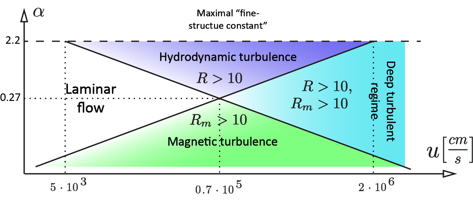
Figure 1: (Colour online) Flow regimes for the electron liquid in a Weyl semimetal on the diagram “fine-structure constant” $\alpha=\frac{e^{2}}{\varkappa\hbar v_{F}}$ vs. flow velocity $u$ (log-log scale) for the room temperature $T=T_{\text{room}}=300K$ and the Fermi velocity $v_{F}=10^{8}\frac{cm}{s}$. The maximum value of the “fine-structure constant” is $\alpha_{max}=\frac{e^{2}}{\hbar v_{F}}\approx 2.2$.

Let us emphasise that the dynamo effect is a macroscopic classical phenomenon. The effect if favoured by large system sizes $L$, which lead to large $R_{m}$. In experiments with solid-state systems the size $L$ is rather limited, with centimetre-size samples being at the upper end of the range accessible for WSMs. Since the effect is not sensitive to quantum interference effects, higher temperatures $T$ are much preferable to maximize $R_{m}$; the room temperature, $T_{\rm room}$, thus represents a reasonable comparison scale. We emphasise that even at room temperature Weyl semimetals are not Maxwell gases and quantum statistics and quantum nature of the electron-electron scattering are important, but quantum coherence is not essential for the dynamo effect. Using these length and temperature scales, we obtain the following estimate for the main figure of merit in the dynamo theory:

$$R_{m}\sim\frac{1}{\alpha^{2}}\frac{e^{2}}{\hbar}\frac{4\pi k_{B}T}{\hbar v_{F}c^{2}}uL\sim\frac{10^{-6}}{\alpha^{2}}\left(\frac{T}{T_{\rm room}}\right)\times u\left[{\rm\frac{cm}{s}}\right]\,L[{\rm cm}],$$ (11)

where $u$ is the typical velocity of the flow.

Now, we turn to estimates of the hydrodynamic Reynolds number 2. The viscosity of the quasiparticles in a Weyl semimetal at temperature $T$ may be estimated as $\eta\sim n(T)T\tau_{\text{rel}}$, where $n(T)$ is the concentration of the thermally excited quasiparticles and $\tau_{\text{rel}}\sim\hbar(\alpha^{2}k_{B}T)^{-1}$ is the momentum relaxation time. Note that this result follows from second-order perturbation theory in Coulomb interaction and neglects screening effects. This leads to

$$\eta\sim\frac{(k_{B}T)^{3}}{\alpha^{2}\hbar^{2}v_{F}^{3}}.$$ (12)

The motion of a Weyl-semimetal liquid is turbulent in the hydrodynamic sense when the term $\frac{w}{v_{F}^{2}}({{\bf u}\cdot\bm{\nabla}}){\bf u}$ in the Navier-Stokes equation (7) dominates the dissipative terms $\sim\eta\nabla^{2}{\bf u}$ that come from the viscosity of the Weyl fluid. This yields the following estimate

$$R=\frac{wuL}{\eta v_{F}^{2}}\sim\alpha^{2}\frac{k_{B}T}{\hbar}\frac{uL}{v_{F}^{2}}\sim 4\alpha^{2}10^{-3}\left(\frac{T}{T_{\rm room}}\right)\times u\left[{\rm\frac{cm}{s}}\right]\,L[{\rm cm}],$$ (13)

where we have used the estimate $w\approx\frac{7g\pi^{2}T^{4}}{90\hbar^{3}v_{F}^{3}}\sim\frac{(k_{B}T)^{4}}{\hbar^{3}v_{F}^{3}}$ for the specific enthalpy at high temperatures.

We note in this context that the viscosity of a Fermi liquid at temperature $T$ may be estimated as $\eta\sim{\varepsilon_{F}^{5}}/({T^{2}\hbar^{2}v_{F}^{3}})$, where $\varepsilon_{F}$ and $v_{F}$ are the Fermi energy and velocity, respectively. Because the hydrodynamic Reynolds number $R\sim\frac{T^{2}}{v_{F}^{2}\varepsilon_{F}\hbar}$ gets rapidly suppressed with increasing the Fermi energy $\varepsilon_{F}$, topological semimetals are indeed a favourable platform for achieving electronic turbulence as compared to “conventional” hydrodynamic metals.

Naturally, the geometry and the magnitude of the velocity field $u$ much depends on the mechanism to stir up hydrodynamic motion and follows from the solution of the Navier-Stoker equations, which is a challenging task in most cases. Furthermore, since observation of a phenomenon of this kind has never been attempted in solid-state materials, it is not clear at the moment what experimental technique would be the most efficient to achieve high hydrodynamic flows – pulsed fields, crossed electric and magnetic fields or just a rapid rotation of the sample are all possibilities to consider. While below we consider in detail one of the standard and simplest dynamo models, we emphasise immediately that the estimates (11) and (13) are not prohibitive; and it is conceivable that relatively large magnetic Reynolds numbers, necessary for the dynamo to commence, are achievable for realistic flow velocities with $u$ of order one kilometre/second or greater (especially considering that the dielectric constant may be as high as $\varkappa\sim 50$ in WSMs), cf. Fig. 1.

Now, we discuss a specific model of dynamo effect – the so-called kinematic Ponomarenko dynamo Ponomarenko ; Jones , with an eye on how the terms in MHD equations, descending from the chiral anomaly, change the effect. The Ponomarenko dynamo does not necessarily represent the most experimentally realistic setup, but it does represent the simplest textbook model, which contains the key qualitative features of a dynamo mechanism and is amenable to analytical analysis.

In order for a dynamo action to occur, the magnetic Reynolds number must exceed a critical value $R^{c}_{m}$ Fitzpatrick (2015). The purpose of the calculation below is to obtain the dependence of the critical Reynolds number, $R^{c}_{m}$, on the helicity term. For simplicity, we neglect the time dependence of the chemical-potential difference $\mu_{L}-\mu_{R}$ on the times we consider.

We re-write Eq. (9) as

$$\frac{\partial{\bf B}}{\partial t}={\bm{\nabla}}\times({\bm{u}}\times{\bf B})+\frac{c^{2}}{4\pi\sigma}\nabla^{2}{\bf B}+\xi{\bm{\nabla}}\times{\bf B},$$ (14)

where $\xi=ge^{2}(\mu_{L}-\mu_{R})/(4\pi^{2}\hbar^{2}\sigma)$. We consider a cylindrical geometry of the sample with a flow field $\mathbf{u}=(0,r\Omega,u_{0})$, where $\Omega$ and $u_{0}$ are constants, for $r\leq a$, and $\mathbf{u}=0$ for $r>a$ Fitzpatrick (2015). Plugging the ansatz $\mathbf{B}(r,\theta,z,t)=\mathbf{B}(r)e^{i(n\theta-kz)+\gamma t}$ into (9), the components of the magnetic field $B_{\pm}=B_{r}\pm iB_{\theta}$ satisfy the equations

$$y^{2}B^{\prime\prime}_{\pm}+yB^{\prime}_{\pm}=\left[q^{2}y^{2}+(n\pm 1)^{2}\right]B_{\pm}$$

$$-\delta\left[nyB^{\prime}_{\mp}\mp n(n\mp 1)B_{\mp}\pm k^{2}a^{2}y^{2}B_{\pm}\mp q^{2}y^{2}B_{r}\right]$$ (15)

for $y=r/a\leq 1$ and

$$y^{2}B^{\prime\prime}_{\pm}+yB^{\prime}_{\pm}=\left[s^{2}y^{2}+(n\pm 1)^{2}\right]B_{\pm}$$ (16)

for $y>1$, where $B^{\prime}_{\pm}$ ($B^{\prime\prime}_{\pm}$) is the first (second) derivative with respect to $y$; $\delta=4\pi\sigma\xi/kc^{2}$, $q^{2}=k^{2}a^{2}+\gamma\tau_{R}+i(n\Omega-ku_{0})$, $s^{2}=k^{2}a^{2}+\gamma\tau_{R}$, where $\tau_{R}=4\pi\sigma a^{2}/c^{2}$ is the time scale of the magnetic field diffusion.

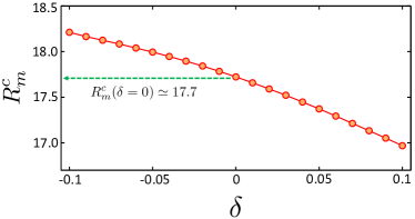
Figure 2: (Colour online) The critical magnetic Reynold number $R_{m}^{c}$ of the $n=1$ kinematic Ponomarenko dynamo as a function of the helicity parameter $\delta=4\pi\sigma\xi/kc^{2}$, with $k$ being the wave-vector of the dynamo instability. $R^{c}_{m}\simeq 17.7$ is the critical value for the dynamo in the absence of helicity. We note that a self-exciting dynamo will always correspond to the chirality with a lower critical Reynolds number. The chiral anomaly, thus, always aids the dynamo effect.

For each mode $n$, the magnetic field starts to grow exponentially when $\mathrm{Re}(\gamma)>0$, which occurs if the magnetic Reynolds number exceeds a critical value $R_{m}^{c}$. In the absence of helicity ($\delta=0$), Eq. (14) reduces to the conventional dynamo equation and the $n=0$ mode is not excited for an arbitrary intensity of the flow Fitzpatrick (2015). For non-zero helicity, we solved the inhomogeneous equations (Dynamo Effect and Turbulence in Hydrodynamic Weyl Metals) and (16) with appropriate boundary conditions imposed sup (2018) to obtain the dispersion relation for the dynamo mode. The obtained values of $R_{m}^{c}$ for a dynamo with $n=1$ and a particular direction of wavevector ${\bf k}$ (the $z$ axis) are shown in Fig. 2. The $n=1$ mode is the leading mode, where the dynamo action commences first, and for which the critical magnetic Reynold number is the smallest and potentially within reach for actual Weyl systems. In the absence of helicity (i.e., if $\delta=0$), it is known to be $R^{c}_{m}\simeq 17.7$ Fitzpatrick (2015). Interestingly enough, the helicity $\delta>0$ reduces the critical value of the magnetic Reynold number for the $n=1$ mode and helps the dynamo action to occur for $R^{c}_{m}<17.7$. Because dynamo flows with various directions of ${\bf k}$ may emerge spontaneously in a turbulent liquid, the presence of helicity (a consequence of the chiral anomaly) would generically aid the dynamo bootstrap in any geometry of the flow.

In conclusion, this paper proposes hydrodynamic Weyl semimetals as a host to electronic turbulence and/or dynamo effect. We derived the Navier-Stokes equations (7) and equations of magnetohydrodynamics (9) and estimated two key figures of merit – the hydrodynamic and magnetic Reynolds numbers. Fig. 1 summarises our findings and shows that both turbulence and dynamo mechanism are in principle experimentally achievable. However, many interesting questions remain, such as experimental signatures of the turbulent electronic motion and the role of “new” terms in the Navier-Stokes equations, descending from the quantum chiral anomaly. Finally, we mention that while three-dimensional Dirac materials are indeed interesting from the perspective of realising the dynamo bootstrap, a number of other electronic materials may also serve as platforms to realize the effect. For example, electronic metals near critical points (e.g., right above a superconducting transition) represent a promising system to look at in this context (both from the perspective of achieving hydrodynamic flows and large Reynolds numbers) and could pave the way to simulating in solid-state materials the effect of magnetic field’s self-excitation – a remarkable phenomenon, usually delegated to the fields of geophysics, astrophysics and cosmology.

Acknowledgements. We are grateful to Matthew Foster, Anton Burkov and Aydin Keser for useful discussions. This research was supported by NSF DMR-1613029 (SS), DOE-BES (DESC0001911) (VG) and the Simons Foundation (VG).

Supplemental Material for
“Dynamo Effect and Turbulence in Hydrodynamic Metals”

I Navier-Stokes equation for a Weyl semimetal

In this section we present a microscopic derivation of the Navier-Stokes equation (7) for a Weyl semimetal. In the absence of dissipation, electromagnetic fields and internodal scattering processes, the motion of the electronic liquid in a Weyl semimetal is Lorentz-invariant with the Fermi velocity $v_{F}$ playing the role of the speed of light $c$. Indeed, so long as the crystal lattice of a Weyl semimetal is at rest, Weyl electrons propagate with velocity $v_{F}$ in all directions regardless of the hydrodynamic velocity ${\bf u}$ of the electron liquid and, thus, obey the relativistic composition law for velocities with the replacement $c\rightarrow v_{F}$.

The dynamics of such a liquid is described by the relativistic Navier-Stokes equation [see, for example, Ref. Landau and Lifshitz, ]. Here, we focus on the interplay of this dynamics with the internodal scattering of electrons (including the chiral anomaly) and electromagnetic fields, which do not transform under representations of the Lorentz group with the speed of light replaced by the Fermi velocity.

In what follows, we set $v_{F}=1$ and, following Refs. Landau and Lifshitz, and Landau and Lifshitz, , introduce the four-position $x^{i}=(t,{\bf r})$ and the four-velocity $u^{i}=\gamma(1,{\bf u})$ of the liquid. The stress-energy tensor of the Weyl electron liquid is given by

$$T^{ij}=\gamma wu^{i}u^{j}-Pg^{ij},$$ (S1)

where $w$ is the enthalpy of the liquid per volume; $P$ is the pressure; $\gamma=\left(1-u^{2}\right)^{\frac{1}{2}}$; and $g^{ij}=\text{diag}\left(1,-1,-1,-1\right)$ is the metric tensor. The equations of motion of quasiparticles near a Weyl node are given by

$$\frac{\partial T^{ij}}{\partial x^{i}}=\frac{1}{c}F^{jk}j_{k}+Q^{j},$$ (S2)

where $F^{ij}$ is the effective electromagnetic-field tensor, which we find below, $j_{k}=(\rho,-{\bf j})$ is the covariant four-current of Weyl fermions near the node under consideration (in this section we suppress the node index), with $\rho$ being the charge density (cf. Eq. 6), and $Q^{i}$ is the effective “force” which comes from the internodal electron dynamics and which we also derive below. In this section, we do not consider dissipation processes due to the viscosity of the electron liquid, as their contribution amounts to the usual viscous force in a relativistic liquidLandau and Lifshitz .

Lorentz force. The contribution $S_{em}=-e\int\phi dt+\frac{e}{c}\int{\bf A}d{\bf r}$ of the electromagnetic field to the action of a Weyl electron corresponds to the effective electromagnetic four-potential $\tilde{A}^{i}=(c\phi,{\bf A})$, defined as $S_{em}=-\frac{e}{c}\int\tilde{A}^{i}dx_{i}$, where $c$ is the speed of light (measured in units of the Fermi velocity $v_{F}$). Using the corresponding electromagnetic-field tensor

$$F^{ij}\equiv\frac{\partial\tilde{A}^{j}}{\partial x_{i}}-\frac{\partial\tilde{A}^{i}}{\partial x_{j}}=\left(\begin{array}[]{cccc}0&-cE_{x}&-cE_{y}&-cE_{z}\\ cE_{x}&0&-B_{z}&B_{y}\\ cE_{y}&B_{z}&0&-B_{x}\\ cE_{z}&-B_{y}&B_{x}&0\end{array}\right),$$ (S7)

we recover the conventional expression $\frac{1}{c}F^{jk}j_{k}=\rho{\bf E}+\frac{1}{c}{\bf j}\times{\bf B}$ for the Lorenz force acting on a unit volume of the Weyl liquid.

Chiral anomaly and internodal scattering. Simultaneous application of parallel electric and magnetic fields in a Weyl semimetal results in the pumping of charge carriers from one node to the other. Impurities and interactions may also lead to internodal scattering. All these internodal processes contribute to the time derivatives $\frac{\partial T^{0i}}{\partial t}$ (where $i=0,x,y,z$), which corresponds to the four-force [cf. Eq. (S2)]

$$Q^{i}=(\gamma q_{w}-q_{P},\gamma q_{w}{\bf u}),$$ (S8)

where

$$q_{w}=\frac{4}{3}\left(\frac{\partial\varepsilon}{\partial\rho}\right)\left(\chi\frac{ge^{3}}{h^{2}c}{\bf E}\cdot{\bf B}-\frac{\rho-\tilde{\rho}}{\tau_{\text{in}}}\right)$$ (S9)

$$q_{P}=\frac{1}{3}\left(\frac{\partial\varepsilon}{\partial\rho}\right)\left(\chi\frac{ge^{3}}{h^{2}c}{\bf E}\cdot{\bf B}-\frac{\rho-\tilde{\rho}}{\tau_{\text{in}}}\right)$$ (S10)

are the the rates of change of the enthalpy and the pressure of charge carriers near a given Weyl node due to internodal processes; $\varepsilon$ and $\chi=\pm 1$ are the internal energy (per volume) and the chirality of Weyl fermions near this node; $\tilde{\rho}$ is the charge density at the other node. In Eqs. (S9) and (S10) we have used that for Weyl fermions $P\approx\varepsilon/3$ and $w\approx 4\varepsilon/3$. The expression $\chi\frac{ge^{3}}{h^{2}c}{\bf E}\cdot{\bf B}-\frac{\rho-\tilde{\rho}}{\tau_{\text{in}}}$ in Eqs. (S9) and (S10) describes the change of the charge $\rho$ density near a node due to the chiral magnetic effect and internodal scattering [cf. Eq. (5)].

The change of the internal energy $\varepsilon$ when changing the number of particles near a node depends on the heat transfer between the respective electrons and the environment. In this paper, we focus on isothermal flows, with the system being kept at a constant temperature $T$, and assume that thermal equilibration near the nodes (e.g. due a phonon bath which may flow together with the electron liquid) takes place significantly faster than the internodal particle-transfer processes. Under these conditions, we find from Eqs. (6) and (8)

$$\left(\frac{\partial\varepsilon}{\partial\rho}\right)=\left(\frac{\partial\varepsilon}{\partial\rho}\right)_{T}=\frac{3\mu}{e}\frac{\mu^{2}+\pi^{2}T^{2}}{3\mu^{2}+\pi^{2}T^{2}}.$$ (S11)

We emphasise, however, that the rate $\left(\frac{\partial\varepsilon}{\partial\rho}\right)$ may, in general, be different under different assumptions about the nature of equilibration processes. For example, if the internodal dynamics is fast compared to internodal equilibration, the former will result in different temperatures or even non-equilibrium distributions of electrons near different nodes.

Navier-Stokes equation. In order to obtain the Navier-Stokes equation, we consider the projection of Eq. (S2) on the direction perpendicular to the four-velocity $u^{i}$:

$$\frac{\partial T^{ji}}{\partial x^{j}}-u^{i}u_{l}\frac{\partial T^{lk}}{\partial x^{l}}=\frac{1}{c}F^{ik}j_{k}-\frac{1}{c}u^{i}u_{n}F^{nk}j_{k}+Q^{i}-u^{i}u_{j}Q^{j}.$$ (S12)

Considering the vector components ($i=x,y,z$) of Eq. (S12) and using Eqs. (S1), (S9) and (S10) and that $u_{i}u^{i}=1$, we arrive at the Navier-Stokes equation

$$w\left(\frac{\partial}{\partial t}+{\bf u}\cdot{\bm{\nabla}}\right){\bf u}=-{\bm{\nabla}}P-{\bf u}\frac{\partial P}{\partial t}+\rho{\bf E}+\frac{1}{c}\,{\bf j}\times{\bf B}+\frac{{\bf u}}{3}\left(\frac{\partial\varepsilon}{\partial\rho}\right)\left(\chi\frac{ge^{3}}{h^{2}c}{\bf E}\cdot{\bf B}-\frac{\rho-\tilde{\rho}}{\tau_{\text{in}}}\right),$$ (S13)

where we neglected corrections of higher orders in ${\bf u}^{2}$ to each term.

II Ponomarenko dynamo and helicity

In this section we provide the details of derivations of equations governing the kinematic Ponomarenko dynamo for a given flow velocity. For completeness in Sec. II.1 we present the conventional Ponomarenko dynamo, and then the effects of helicity are examined in Sec. II.2.

II.1 Conventional Ponomarenko Dynamo

The dynamo equation reads as

$$\frac{\partial\mathbf{B}}{\partial t}=\mathbf{B}\cdot\bm{\nabla}\mathbf{u}-\mathbf{u}\cdot\bm{\nabla}\mathbf{B}+\frac{c^{2}}{4\pi\sigma}\nabla^{2}\mathbf{B}.$$ (S14)

Following Ref. [Fitzpatrick, 2015], we assume that a cylinder is filled up with a conductive liquid with a flow field as

$$\mathbf{u}=\begin{cases}(0,r\Omega,u_{0})&r\leq a\\ 0&r\geq a\end{cases},$$

where $a$ is the radius of the cylinder, $\Omega$ is the angular velocity and $u_{0}$ is the velocity along the axis, all taken to be constant. Assuming the ansatz

$$\mathbf{B}(r,\theta,z,t)=\mathbf{B}(r)e^{i(n\theta-kz)+\gamma t}$$ (S15)

for the magnetic field and plugging into the dynamo equation, we obtain the $r$- and $\theta$- components of the magnetic fields as

$$y^{2}\frac{d^{2}B_{r}}{dy^{2}}+y\frac{dB_{r}}{dy}=(q^{2}y^{2}+n^{2}+1)B_{r}+2inB_{\theta},$$ (S16)

$$y^{2}\frac{d^{2}B_{\theta}}{dy^{2}}+y\frac{dB_{\theta}}{dy}=(q^{2}y^{2}+n^{2}+1)B_{\theta}-2inB_{r},$$ (S17)

The $z$-component of the magnetic field doesn’t enter the equations above. It can be determined from $\bm{\nabla}\cdot\mathbf{B}=0$. Letting $B_{\pm}=B_{r}\pm B_{\theta}$, we get a set of separable equations

$$y^{2}\frac{d^{2}B_{\pm}}{dy^{2}}+y\frac{dB_{\pm}}{dy}-[q^{2}y^{2}+(n\pm 1)^{2}]B_{\pm}=0,~{}~{}~{}y\leq a,$$ (S18)

$$y^{2}\frac{d^{2}B_{\pm}}{dy^{2}}+y\frac{dB_{\pm}}{dy}-[s^{2}y^{2}+(n\pm 1)^{2}]B_{\pm}=0,~{}~{}~{}y>a,$$ (S19)

where

$$y=\frac{r}{a},~{}~{}\tau_{R}=\frac{4\pi\sigma a^{2}}{c^{2}},~{}~{}q^{2}=k^{2}a^{2}+\gamma\tau_{R}+i(n\Omega-ku_{0})\tau_{R},~{}~{}s^{2}=k^{2}a^{2}+\gamma\tau_{R}.$$ (S20)

Equations (S18-S19) are modified Bessel equations with the solutions

$$B_{\pm}(y)=C_{\pm}\frac{I_{n\pm 1}(qy)}{I_{n\pm 1}(q)},~{}~{}~{}y\leq 1,$$ (S21)

$$B_{\pm}(y)=D_{\pm}\frac{K_{n\pm 1}(sy)}{K_{n\pm 1}(s)},~{}~{}~{}y>1,$$ (S22)

where $I_{n}$ and $K_{n}$ are modified Bessel functions. Continuity of the fields across the boundary yields $C_{\pm}=D_{\pm}$. The second matching condition is given due the jumping of angular velocity across the boundary:

$$\left[\frac{dB_{\pm}}{dy}\right]^{y=1_{+}}_{y=1_{-}}=\pm i\Omega\tau_{R}\left(\frac{B_{+}+B_{-}}{2}\right).$$ (S23)

Inserting the solutions (S21) and (S22) in the equations above, we obtain the dispersion relation as

$$G_{+}G_{-}=\frac{i}{2}\Omega\tau_{R}(G_{+}-G_{-}),$$ (S24)

where

$$G_{\pm}=q\frac{I^{\prime}_{n\pm 1}(q)}{I_{n\pm 1}(q)}-s\frac{K^{\prime}_{n\pm 1}(s)}{K_{n\pm 1}(s)}.$$ (S25)

Here, ^′ denotes derivative with respect to the argument.

Our aim would be to obtain the magnetic Reynold number $R_{m}=\tau_{R}/\tau_{H}$, where $\tau_{H}=a/v$. Here $v$ denotes the typical velocity of the flow. Taking $v=\sqrt{\Omega^{2}a^{2}+u^{2}_{0}}$, the $R_{m}$ reads as

$$R_{m}=\frac{\tau_{R}\sqrt{\Omega^{2}a^{2}+u^{2}_{0}}}{a}.$$ (S26)

To find the critical magnetic Reynold number $R^{c}_{m}$, beyond which the dynamo action commences, we have to solve equation (S24) numerically. We set $\mathrm{Re}(\gamma)=0$, the onset value beyond which the magnetic field grows exponentially for $\mathrm{Re}(\gamma)>0$. We vary $ka$ and $\mathrm{Im}(\gamma\tau_{R})$ over a wide range of values and look for unknown variables $\Omega\tau_{R}$ and $u_{0}\tau_{R}/a$, all dimensionless, through the imaginary and real parts of the dispersion relation (S24). The $n=1$ is the first dynamo mode excited with $R^{c}_{m}\simeq 17.72$.

II.2 Ponomarenko dynamo with helicity term

Now we add the helical term to the dynamo equation as

$$\frac{\partial\mathbf{B}}{\partial t}=\mathbf{B}\cdot\bm{\nabla}\mathbf{u}-\mathbf{u}\cdot\bm{\nabla}\mathbf{B}+\frac{c^{2}}{4\pi\sigma}\nabla^{2}\mathbf{B}+\xi\bm{\nabla}\times\mathbf{B}.$$ (S27)

In writing down the last term we assumed that the $\xi$ is constant to simplify the subsequent equations. In principle it does depend on the magnetic and electric fields. The last term $\bm{\nabla}\times\mathbf{B}$ gives rise to new terms involving $B_{z}$:

$$\left[\frac{in}{r}B_{z}(r)+ikB_{\theta}(r)\right]e^{i(n\theta-kz)+\gamma t}$$ (S28)

in the $r$-component and

$$\left[-ikB_{r}(r)-\frac{\partial{B_{z}(r)}}{\partial r}\right]e^{i(n\theta-kz)+\gamma t}$$ (S29)

in the $\theta$-component, which are added to right hand side of Eqs. (S16) and (S17), respectively.

Using $\bm{\nabla}\cdot\mathbf{B}=0$, we write the $z$-component as

$$B_{z}(r)=\frac{1}{ikr}B_{r}(r)+\frac{1}{ik}\frac{dB_{r}(r)}{dr}+\frac{n}{kr}B_{\theta}(r)$$ (S30)

$$y^{2}\frac{d^{2}B_{r}}{dy^{2}}+y\frac{dB_{r}}{dy} = (q^{2}y^{2}+n^{2}+1)B_{r}+2inB_{\theta}-\delta\left(nB_{r}+ny\frac{dB_{r}}{dy}+in^{2}B_{\theta}+ik^{2}a^{2}y^{2}B_{\theta}\right),$$ (S31)

$$y^{2}\frac{d^{2}B_{\theta}}{dy^{2}}+y\frac{dB_{\theta}}{dy} = (q^{2}y^{2}+n^{2}+1)B_{\theta}-2inB_{r}-\delta\left(-ik^{2}a^{2}y^{2}B_{r}-iB_{r}+iy\frac{dB_{r}}{dy}+iy^{2}\frac{d^{2}B_{r}}{dy^{2}}+nB_{\theta}-ny\frac{dB_{\theta}}{dy}\right)$$

where $\delta=\tau_{R}/\tau_{c}$ with $\tau_{c}=ka^{2}/\xi$. In the limit $\xi=0$ ($\delta\rightarrow 0$) the equations above reduce to Eqs. (S16) and (S17). In (LABEL:Bt_chi) we replace the $y^{2}\frac{d^{2}B_{r}}{dy^{2}}+y\frac{dB_{r}}{dy}$ in the parentheses with the expression (S31) and keep the terms up to first order in $\delta$. We get

$$y^{2}\frac{d^{2}B_{r}}{dy^{2}}+y\frac{dB_{r}}{dy} = (q^{2}y^{2}+n^{2}+1)B_{r}+2inB_{\theta}-\delta\left(nB_{r}+ny\frac{dB_{r}}{dy}+in^{2}B_{\theta}+ik^{2}a^{2}y^{2}B_{\theta}\right),$$ (S33)

$$y^{2}\frac{d^{2}B_{\theta}}{dy^{2}}+y\frac{dB_{\theta}}{dy} = (q^{2}y^{2}+n^{2}+1)B_{\theta}-2inB_{r}-\delta\left(-ik^{2}a^{2}y^{2}B_{r}+i(q^{2}y^{2}+n^{2})B_{r}-nB_{\theta}-ny\frac{dB_{\theta}}{dy}\right)$$ (S34)

Rewriting the equations above in terms of $B_{\pm}=B_{r}\pm iB_{\theta}$, we obtain

$$y^{2}\frac{d^{2}B_{+}}{dy^{2}}+y\frac{dB_{+}}{dy} = \left[q^{2}y^{2}+(n+1)^{2}\right]B_{+}-\delta\left(ny\frac{dB_{-}}{dy}-n(n-1)B_{-}+k^{2}a^{2}y^{2}B_{+}-q^{2}y^{2}B_{r}\right),$$ (S35)

$$y^{2}\frac{d^{2}B_{-}}{dy^{2}}+y\frac{dB_{-}}{dy} = \left[q^{2}y^{2}+(n-1)^{2}\right]B_{-}-\delta\left(ny\frac{dB_{+}}{dy}+n(n+1)B_{+}-k^{2}a^{2}y^{2}B_{-}+q^{2}y^{2}B_{r}\right).$$ (S36)

In order to examine the effect of helicity $\delta$ on the magnetic Reynold number, in what follows we use equations (S35) and (S36) to evaluate the $R^{c}_{m}$ discussed in the preceding subsection.

We rewrite the equations as

$$y^{2}\frac{d^{2}B_{+}}{dy^{2}}+y\frac{dB_{+}}{dy} = \left[q_{+}^{2}y^{2}+(n+1)^{2}\right]B_{+}-\delta\left(ny\frac{dB_{-}}{dy}-n(n-1)B_{-}-\frac{q^{2}y^{2}}{2}B_{-}\right),$$ (S37)

$$y^{2}\frac{d^{2}B_{-}}{dy^{2}}+y\frac{dB_{-}}{dy} = \left[q_{-}^{2}y^{2}+(n-1)^{2}\right]B_{-}-\delta\left(ny\frac{dB_{+}}{dy}+n(n+1)B_{+}+\frac{q^{2}y^{2}}{2}B_{+}\right),$$ (S38)

where

$$q_{+}^{2}=\left(1+\frac{\delta}{2}\right)q^{2}-\delta k^{2}a^{2},~{}~{}~{}q_{-}^{2}=\left(1-\frac{\delta}{2}\right)q^{2}+\delta k^{2}a^{2}.$$ (S39)

Without the terms in the parentheses in the right side, we have a set of homogenous equations with helicity included.

$$y^{2}\frac{d^{2}B_{0,+}}{dy^{2}}+y\frac{dB_{0,+}}{dy} = \left[q_{+}^{2}y^{2}+(n+1)^{2}\right]B_{0,+},$$ (S40)

$$y^{2}\frac{d^{2}B_{0,-}}{dy^{2}}+y\frac{dB_{0,-}}{dy} = \left[q_{-}^{2}y^{2}+(n-1)^{2}\right]B_{0,-}.$$ (S41)

Theses are modified Bessel equations with solutions

$$B_{0,\pm}(y)\propto I_{n\pm 1}(q_{\pm}y),K_{n\pm 1}(q_{\pm}y).$$ (S42)

Using the above homogenous solutions, we use the perturbation theory to solve the equations in (S37-S38). We write the solutions up to the first order in $\delta$ as

$$B_{+}(y)=B_{0,+}(y)+\delta A_{+}(y),~{}~{}~{}B_{-}(y)=B_{0,-}(y)+\delta A_{-}(y),$$ (S43)

Plugging (S43) into the equations (S37-S38), we obtain

$$y^{2}\frac{d^{2}A_{+}}{dy^{2}}+y\frac{dA_{+}}{dy} = \left[q_{+}^{2}y^{2}+(n+1)^{2}\right]A_{+}-\left(ny\frac{dB_{0,-}}{dy}-n(n-1)B_{0,-}-\frac{q^{2}y^{2}}{2}B_{0,-}\right),$$ (S44)

$$y^{2}\frac{d^{2}A_{-}}{dy^{2}}+y\frac{dA_{-}}{dy} = \left[q_{-}^{2}y^{2}+(n-1)^{2}\right]A_{-}-\left(ny\frac{dB_{0,+}}{dy}+n(n+1)B_{0,+}+\frac{q^{2}y^{2}}{2}B_{0,+}\right).$$ (S45)

We set $n=1$. Using the standard approaches for solving the non-homogeneous differential equations, and after a lengthy but straightforward calculations, we obtain

$$A_{+}(y)\simeq\left(\frac{q^{2}-q^{2}_{-}}{12}y^{4}+\frac{3q^{2}q_{-}^{2}+q_{+}^{2}(q^{2}-q^{2}_{-})}{192}y^{6}\right)$$ (S46)

$$A_{-}(y)\simeq-\frac{q_{+}^{2}}{32}y^{4}.$$ (S47)

Matching the fields across the boundary at $y=1$, we obtain a dispersion relation, which reads as

$$G_{+}+\delta G\left(A^{y=1}_{+}s\frac{K^{\prime}_{2}(s)}{K_{2}(s)}-A^{\prime y=1}_{+}\right)=-i\Omega\tau_{R}\left(1-G+\delta A^{y=1}_{-}-\delta GA^{y=1}_{+}\right),$$ (S48)

where

$$G=\frac{G_{+}-\delta\left(A^{y=1}_{-}s\frac{K^{\prime}_{0}(s)}{K_{0}(s)}-A^{\prime y=1}_{-}\right)}{G_{-}-\delta\left(A^{y=1}_{+}s\frac{K^{\prime}_{2}(s)}{K_{2}(s)}-A^{\prime y=1}_{+}\right)}.$$ (S49)

Again we solve the dispersion relation (S48) numerically to obtain $R_{m}^{c}$; the results are shown in Fig. 2 in the main text.

References

- Larmor (1919) J. Larmor, “How could a rotating body such as the Sun become a magnet?” Reports of the British Association 87, 159 (1919).
- (2) A. A. Ruzmaikin, D. D. Sokoloff, and Ya. B. Zeldovich, “The Almighty Chance,” World Scientific Lecture Notes in Physics (1990).
- Gilbert (a) A.D. Gilbert, “Dynamo theory,” in Handbook of mathematical fluid dynamics (eds. S. Friedlander and D. Serre), vol. 2, 355-441. Elsevier Science BV (2003) (a).
- Gilbert (b) A.D. Gilbert, in Chapter 1 of Mathematical Aspects of Natural Dynamos, eds E. Dormy and A.M. Soward, CRC Press, (2007) (b).
- (5) L. D. Landau and E. M. Lifshitz, Fluid Mechanics: Volume 6 (Course of Theoretical Physics), Butterworth-Heinemann; 2 edition (1987).
- (6) Yu. B. Ponomarenko, “On the theory of hydromagnetic dynamo,” J. Appl. Mech. Tech. Phys. 14, 775 (1973).
- (7) D.P. Lathrop and C.B. Forest, “Magnetic dynamos in the lab,” Physics Today 64, 40 (2011).
- (8) C. A. Jones, “Course 2: Dynamo Theory,” (Lecture Notes of the Les Houches Summer School 2007), Ph. Cardin and L.F. Cugliandolo, eds. Les Houches, Session LXXXVIII, Published by Elsevier (2008).
- (9) F. Krause and K-H Rädler, “Mean field magnetohydrodynamics and dynamo theory,” Pergamon Press, New-York, (1980).
- (10) E. N. Parker, “Hydromagnetic dynamo models,” Astrophys. J. 122, 293, (1955).
- (11) V. M. Galitski and D. D. Sokoloff, “Kinematic dynamo wave in the vicinity of the solar poles,” Geophysical and Astrophysical Fluid Dynamics 91, 147 (1999).
- Gailitis et al. (2000) Agris Gailitis, Olgerts Lielausis, Sergej Dement’ev, Ernests Platacis, Arnis Cifersons, Gunter Gerbeth, Thomas Gundrum, Frank Stefani, Michael Christen, Heiko Hänel, and Gotthard Will, “Detection of a flow induced magnetic field eigenmode in the riga dynamo facility,” Phys. Rev. Lett. 84, 4365 (2000).
- Spence et al. (2007) E. J. Spence, M. D. Nornberg, C. M. Jacobson, C. A. Parada, N. Z. Taylor, R. D. Kendrick, and C. B. Forest, “Turbulent diamagnetism in flowing liquid sodium,” Phys. Rev. Lett. 98, 164503 (2007).
- Monchaux et al. (2007) R. Monchaux, M. Berhanu, M. Bourgoin, M. Moulin, Ph. Odier, J.-F. Pinton, R. Volk, S. Fauve, N. Mordant, F. Pétrélis, A. Chiffaudel, F. Daviaud, B. Dubrulle, C. Gasquet, L. Marié, and F. Ravelet, “Generation of a magnetic field by dynamo action in a turbulent flow of liquid sodium,” Phys. Rev. Lett. 98, 044502 (2007).
- (15) A. V. Andreev, Steven A. Kivelson, and B. Spivak, “Hydrodynamic description of transport in strongly correlated electron systems,” Phys. Rev. Lett. 106, 256804 (2011).
- (16) Andrew Lucas and Sean A. Hartnoll, “Resistivity bound for hydrodynamic bad metals,” Proc. Natl. Acad. Sci. US 114, 11344 (2017).
- (17) Andrew Lucas and Sankar Das Sarma, “Electronic sound modes and plasmons in hydrodynamic two-dimensional metals,” Phys. Rev. B 97, 115449 (2018).
- (18) Xue-Yang Song, Chao-Ming Jian, and Leon Balents, “A strongly correlated metal built from Sachdev-Ye-Kitaev models,” Phys. Rev. Lett. 119, 216601 (2017).
- (19) Sean A. Hartnoll, Andrew Lucas, and Subir Sachdev, “Holographic quantum matter,” The MIT Press (2018).
- (20) R. Krishna Kumar, D. A. Bandurin, F. M. D. Pellegrino, Y. Cao, A. Principi, H. Guo, G. H. Auton, M. Ben Shalom, L. A. Ponomarenko, G. Falkovich, K. Watanabe, T. Taniguchi, I. V. Grigorieva, L. S. Levitov, M. Polini, and A. K. Geim, “Superballistic flow of viscous electron fluid through graphene constrictions,” Nature Physics 13, 1182 (2017).
- Gooth et al. (2017) Johannes Gooth, Anna Corinna Niemann, Tobias Meng, Adolfo G. Grushin, Karl Landsteiner, Bernd Gotsmann, Fabian Menges, Marcus Schmidt, Chandra Shekhar, Vicky Sueb, Claudia Felser Ruben Huehne, andBernd Rellinghaus, Binghai Yan, and Kornelius Nielsch, “Experimental signatures of the mixed axial-gravitational anomaly in the Weyl semimetal NbP,” Nature 547, 324 (2017).
- (22) J. Gooth, F. Menges, C. Shekhar, V. Sueb, N. Kumar, Y. Sun, U. Drechsler, R. Zierold, C. Felser, and B. Gotsmann, “Electrical and Thermal Transport at the Planckian Bound of Dissipation in the Hydrodynamic Electron Fluid of WP2,” arXiv:1706.05925 (2017).
- (23) Chenguang Fu, Thomas Scaffidi, Jonah Waissman, Yan Sun, Rana Saha, Sarah J. Watzman, Abhay K. Srivastava, Guowei Li, Walter Schnelle, Peter Werner, Machteld E. Kamminga, Subir Sachdev, Stuart S. P. Parkin, Sean A. Hartnoll, Claudia Felser, and Johannes Gooth, “Thermoelectric signatures of the electron-phonon fluid in PtSn4,” arXiv:1802.09468 (2018).
- (24) Matthew S. Foster and Igor L. Aleiner, “Slow imbalance relaxation and thermoelectric transport in graphene,” Phys. Rev. B 79, 085415 (2009).
- Nielsen and Ninomiya (1981) H. B. Nielsen and M. Ninomiya, “Absence of neutrinos on a lattice: (i). proof by homotopy theory,” Nucl. Phys. B 185, 20 – 40 (1981).
- Adler (1969) S. L. Adler, “Axial-vector vertex in spinor electrodynamics,” Phys. Rev. 177, 2426 (1969).
- Bell and Jackiw (1969) J. S. Bell and R. Jackiw, “A pcac puzzle: in the -model,” Il Nuovo Cimento A 60, 47 (1969).
- Son and Spivak (2013) D. T. Son and B. Z. Spivak, “Chiral anomaly and classical negative magnetoresistance of weyl metals,” Phys. Rev. B 88, 104412 (2013).
- Burkov (2018) A. A. Burkov, “Weyl metals,” Annu. Rev. Cond. Mat. Phys. 9, 395 (2018).
- Burkov (2014) A. A. Burkov, “Chiral Anomaly and Diffusive Magnetotransport in Weyl Metals,” Phys. Rev. Lett. 113, 247203 (2014).
- Narozhny et al. (2017) B. N. Narozhny, I. V. Gornyi, A. D. Mirlin, and J. Schmalian, “Hydrodynamic Approach to Electronic Transport in Graphene,” Annalen der Physik 529, 1700043 (2017), arXiv:1704.03494 [cond-mat.mes-hall] .
- Fukushima et al. (2008) Kenji Fukushima, Dmitri E. Kharzeev, and Harmen J. Warringa, “Chiral magnetic effect,” Phys. Rev. D 78, 074033 (2008).
- Kharzeev et al. (2013) D. Kharzeev, K. Landsteiner, A. Schmitt, and H.-U. Yee, eds., Lecture Notes in Physics, Berlin Springer Verlag, Lecture Notes in Physics, Berlin Springer Verlag, Vol. 871 (2013).
- Rodionov and Syzranov (2015) Y. I. Rodionov and S. V. Syzranov, “Conductivity of a Weyl semimetal with donor and acceptor impurities,” Phys. Rev. B 91, 195107 (2015), arXiv:1503.02078 [cond-mat.mes-hall] .
- sup (2018) See Supplemental Material at [URL will be inserted by publisher] for a detailed derivation of the Navier-Stokes equation and Ponomarenko dynamo in the presence of helicity terms. (2018).
- Gorbar et al. (2018) E. V. Gorbar, V. A. Miransky, I. A. Shovkovy, and P. O. Sukhachov, “Consistent hydrodynamic theory of chiral electrons in Weyl semimetals,” Phys. Rev. B 97, 121105 (2018).
- Yamamoto (2016) N. Yamamoto, “Chiral transport of neutrinos in supernovae: Neutrino-induced fluid helicity and helical plasma instability,” Phys. Rev. D 93, 065017 (2016), arXiv:1511.00933 [astro-ph.HE] .
- Hosur et al. (2012) Pavan Hosur, S. A. Parameswaran, and Ashvin Vishwanath, “Charge transport in weyl semimetals,” Phys. Rev. Lett. 108, 046602 (2012).
- Fitzpatrick (2015) Richard Fitzpatrick, Plasma Physics: An Introduction (Taylor and Francis Group, 2015).

References

- (1) L. D. Landau and E. M. Lifshitz, Fluid Mechanics: Volume 6 (Course of Theoretical Physics), Butterworth-Heinemann; 2nd edition (1987)
- (2) L. D. Landau and E. M. Lifshitz, Fluid Mechanics: Volume 2 (Course of Theoretical Physics), Pergamon Press; 5th edition (1967)
- Fitzpatrick (2015) Richard Fitzpatrick, Plasma Physics: An Introduction (Taylor and Francis Group, 2015)