Wireless Quantization Index Modulation: Enabling Communication Through Existing Signals

Abstract – As the number of IoT devices continue to exponentially increase and saturate the wireless spectrum, there is a dire need for additional spectrum to support large networks of wireless devices. Over the past years, many promising solutions have been proposed but they all suffer from the drawback of new infrastructure costs, setup and maintenance, or are difficult to implement due to FCC regulations. In this paper, we propose a novel Wireless Quantization Index Modulation (QIM) technique which uses existing infrastructure to embed information into existing wireless signals to communicate with IoT devices with negligible impact on the original signal and zero spectrum overhead. We explore the design space for wireless QIM and evaluate the performance of embedding information in TV, FM and AM radio broadcast signals under different conditions. We demonstrate that we can embed messages at up to 8–200 kbps with negligible impact on the audio and video quality of the original FM, AM and TV signals respectively.

I Introduction

Over the last decade, we have witnessed a rapid growth in the deployment of IoT devices. By some estimates, there will be more than 26 billion connected IoT devices by the year 2020 [1]. However, as more devices connect to wireless networks, available spectrum is insufficient and existing wireless protocols are ill-equipped to support the growing number of devices. To understand the challenge, consider a home with wireless cameras, security sensor, smart watches, fitness trackers and wireless speakers. These devices use Wi-Fi/Bluetooth or proprietary wireless in the 2.4 GHz ISM band and operate alongside Wi-Fi routers, smartphones, laptops and tablets. As more devices share the wireless channel, wireless interference and packet collisions increase, negatively impacting the throughput and latency [2] [3].

As wireless spectrum (such as the 2.4 GHz ISM band) becomes crowded, conventional wisdom dictates that we migrate to new protocols in less congested wireless channels. New protocols such as 802.11ah, LoRaWAN [4], SIGFOX [5] operate in 915 MHz ISM band, high speed 802.11 n/ac Wi-Fi is moving to 5.8 GHz ISM band, NB-IoT operates in the licensed cellular bands and TV white space networking [6] operates in unused channels in the TV UHF spectrum. Although these solutions are a step in the right direction, let’s discuss these approaches in terms of cost and spectrum utilization.

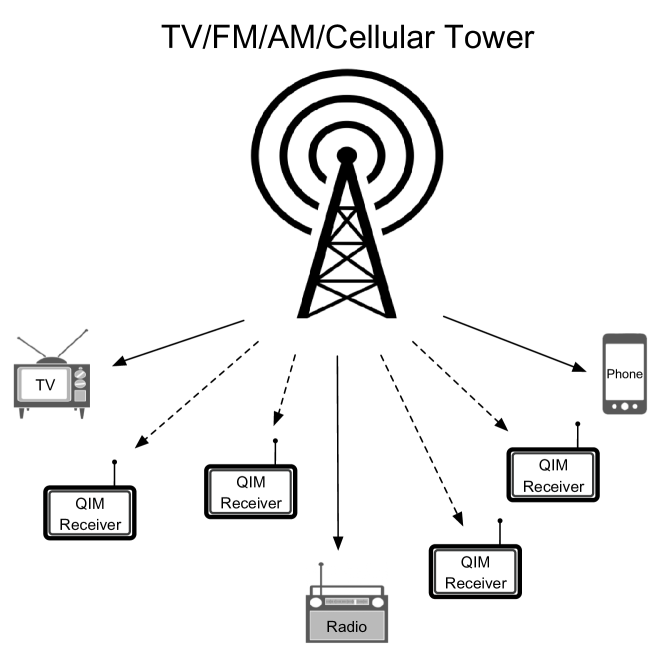
Figure 1: QIM deployment. QIM uses existing wireless signals to communicate with IoT devices.

• Infrastructure and Maintenance Costs: Migration to new protocols such as LoRaWAN, SIGFOX or 802.11ah require setup, deployment and maintenance of dedicated expensive gateways and base stations. Instead, if we can reuse existing wireless infrastructure for communication, we could develop a far simpler and cost effective solution.

• Spectrum Utilization: Wireless spectrum is an extremely valuable and highly regulated resource. TV white space networking uses allocated but otherwise under-utilized TV spectrum for wireless communication. However, more often than not the availability of unused TV channels in urban areas are scarce and it is very cumbersome and expensive to deploy a TV whitespace network [7]. New protocols such as LoRaWAN, SIGFOX, and 802.11ah are moving to the less crowded 915 MHz ISM band, but over time as the number of devices increase, they are going to run into familiar interference and capacity issues: as the number of devices increase, the spectrum is going to become more crowded and eventually saturate. Unless new spectrum is made available, using traditional methods, it is impossible to scale beyond a certain point.

In this paper, we propose a new cost and spectrally efficient solution for wireless communication. Consider an urban city environment as shown in Fig. 1 with existing deployments of AM, FM, TV, and cellular base stations. These base stations have been setup with tremendous infrastructure cost, undergo periodic maintenance and pay licensing fees to transmit at pre-assigned licensed frequencies. The base stations are designed and geographically located for optimal signal coverage. For example, a typical FM tower can be received up to 100 kms.

We introduce Wireless Quantization Index Modulation (QIM), a communication technique which leverages existing infrastructure and reuses broadcast signals to provide additional communication channels for IoT devices. To understand Wireless QIM, without the loss of generality, let’s consider a broadcast TV station. A TV transmitter can use the QIM technique in its baseband to embed a message into the broadcast TV signal by introducing small perturbations while having a negligible impact on the broadcasted TV signal. Legacy TV receivers in the coverage area decode the broadcasted signal as before while IoT devices with a QIM receiver can decode the embedded message without any prior knowledge of the broadcast signal. So, in summary with a small modification to the baseband of the broadcast station, Wireless QIM reuses infrastructure, spectrum and broadcast signals to simultaneously communicate with QIM enabled IoT devices and legacy AM/FM/TV/cellular devices.

Wireless communication requires both uplink and downlink. However, more often than not, it’s asymmetric i.e. depending on the application, either uplink or downlink communication dominates. In this paper, we focus on downlink heavy applications and design a Wireless QIM system for downlink communication. Our target application is a smart city where using Wireless QIM, existing wireless infrastructure provides connectivity for real-time update of electronic bus schedule displays, billboard signs and advertisements, traffic alerts to name a few. With a minimal change in the baseband of existing broadcast towers, we can embed data to wirelessly update devices with a QIM receiver in real-time. These applications would require a minimal uplink channel to send acknowledgement messages, however such a low bandwidth and infrequent task can be accomplished using traditional LoRa, SigFox or cellular radios for the time being. In future work, we will extend the Wireless QIM technique to uplink communication and develop a bi-directional communication system which can leverage existing infrastructure and communicate with smart devices with zero spectrum overhead and minimal additional cost to target a broader set of applications.

To demonstrate the efficacy of Wireless QIM for these applications, we extensively evaluate the design space and explore various tradeoffs between performance of the message and host signal. We implement Wireless QIM on three existing infrastructure broadcast signals: AM, FM, and TV and show that information can be reliably embedded with negligible impact on audio (AM and FM) and video (TV) quality of the host signals. Our results show that using Wireless QIM, we can embed messages for IoT devices at up to 8 kbps in AM radio signals and 200 kbps in FM signals.

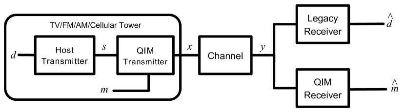
Figure 2: QIM embedding model, where a message $m$ is embedded in a host signal $s$ using the QIM embedding function. The signal passes through a noisy channel and the decoder retrieves the estimated message $\hat{m}$ from the received signal, $y$.

II Quantization Index Modulation

Quantization Index Modulation (QIM) was originally introduced as a scheme for information hiding and digital watermarking [8]. In these applications, a message signal is embedded inside another signal called the host signal such that the embedded message is robust to common degradations, while the host signal suffers minimal degradation. QIM technique achieves an efficient tradeoff between the data rate of the message signal, distortion, and robustness of embedding.

In this work, we use QIM for wireless communication. We show how to embed messages for IoT devices inside existing wireless signals at existing wireless transmitters such that IoT devices with QIM receivers can decode the messages while the broadcasted wireless signal experiences minimal degradation. Fig. 2 shows the block diagram for a typical Wireless QIM system. At the AM/FM/TV/cellular broadcast, data $d$ needs to be transmitted and is passed through the host transmitter to generate a baseband host signal $s$. The host signal can be of any form, for instance, a frequency modulated signal from a FM station. Now, we also want to embed a message $m$ intended for IoT devices. The host signal is passed through a baseband QIM transmitter that uses a quantizer $Q(s)$ to embed the message inside the host signal. This generates a composite signal $x$ that propagates through the (noisy) channel and signal $y$ is received at the receiver. A legacy device would use standard compliant host receiver to decode the host signal, while an IoT device would use a QIM receiver to decode the embedded message $m$. QIM is designed to ensure that both the IoT and legacy devices can decode the desired signals with minimal degradation.

A Wireless QIM system consists of a QIM transmitter at the base station and a QIM receiver at the IoT device. To understand how Wireless QIM works, we will first describe the QIM transmitter followed by the QIM receiver.

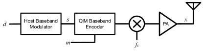
Figure 3: Block diagram of a QIM enabled transmitter.

II-A QIM Transmitter

On a high level, a QIM transmitter embeds information by using a form of quantization to introduce small perturbations in the host signal. Fig. 3 shows the block diagram of a QIM transmitter, where data $d$ is passed through the baseband host modulator to generate the host signal $s$. Then the host signal and message $m$ are passed through the QIM encoder to generate a composite signal $x$ in baseband. Finally, the composite signal is upconverted to carrier frequency $f_{c}$ and transmitted. The implementation of the baseband QIM encoder depends on the host signal. For analog systems such as AM radio, QIM encoder consists of the digital baseband followed by the ADC, a standard component. Whereas in digital FM radio and TV systems, the QIM encoder can be integrated into pre-existing digital baseband. In the following section we explain how the QIM embedding process works. First lets define a uniform quantizer $Q\left(s\right)$ as

$$\vspace{-2pt}Q(s)=\Delta\cdot round(\frac{s}{\Delta})\vspace{-2pt}$$ (1)

where $\Delta$ is the quantization step size and is defined as

$$\vspace{-2pt}\Delta=\frac{2\cdot max(s)}{N}\vspace{-2pt}$$ (2)

Here $N$ is the number of quantization levels. The step size and number of levels determine the embedding resolution for the host signal. Quantizer Q(s) can now be used to define the QIM embedding function,

$$\vspace{-2pt}Q_{m}(s)=Q(s-d_{m})+d_{m}\vspace{-2pt}$$ (3)

where $d_{m}$ is the dither, a function of the message $m$ that is applied to the host signal. $d_{m}$ can take one of the two following values to represent embedding of either a 0-bit or 1-bit.

$$\vspace{-2pt}d_{1}=\pm\frac{\Delta}{4}\text{ and }d_{0}=\begin{cases}d_{1}+\frac{\Delta}{2},&\text{if }d_{1}\leq 0\\ d_{1}-\frac{\Delta}{2},&\text{otherwise}\end{cases}\vspace{-2pt}$$ (4)

The equation shows that if the 1-bit dither is negative, $d_{1}$ = $\nicefrac{{-\Delta}}{{4}}$, then 0-bit dither, $d_{0}$ = $\nicefrac{{\Delta}}{{4}}$, will be a positive value. Similarly, for a positive 1-bit dither, the 0-bit dither would be a negative value. So, in summary we create two dithered quantizers to embed data in the host signal which is dependent on the bit value of the embedded message $m$.

Fig. 4 illustrates this QIM embedding process for a positive 1-bit dither $d_{1}$ with $N=4$ levels, represented by solid horizontal lines. The dashed horizontal lines represent quantization levels for the 1-bit dithered quantizer and dotted lines for the 0-bit quantizer, defined by Eq. 3. We can see that because the dither for a 1-bit is defined as $\nicefrac{{\Delta}}{{4}}$, the dashed lines are shifted up by $\nicefrac{{\Delta}}{{4}}$ from the original set of levels and vise versa for 0-bit quantizer.

Each sample point of the host signal (dashed green line) is perturbed to the appropriate level depending on the message $m$ (shown at the top of the figure). For instance, at the first highlighted sample point (green dot) we encode a 0-bit and the composite signal (solid blue line) goes down to $\nicefrac{{-5\Delta}}{{4}}$, the nearest 0-bit level (blue X). Similarly, at the second highlighted point we embed a 1-bit, which jumps up to $\nicefrac{{5\Delta}}{{4}}$, the nearest level for a 1-bit. We can see from the example that the distance between quantization points is uniformly distributed between [$\nicefrac{{\Delta}}{{2}}$, $\nicefrac{{-\Delta}}{{2}}$]. As a result, the mean error due to embedding is equal to $\nicefrac{{\Delta^{2}}}{{12}}$.

Finally, we characterize the impact of the QIM encoder on the host signal. We define distortion in the host signal by comparing the original host signal to the composite signal generated by embedding and can be expressed as,

$$\vspace{-2pt}D_{s}=\frac{1}{K}\sum_{i=1}^{K}|s_{i}-x_{i}|^{2}\vspace{-2pt}$$ (5)

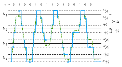
Figure 4: Embedding using QIM for $d_{1}=\frac{\Delta}{4}$ and $d_{0}=\frac{-\Delta}{4}$

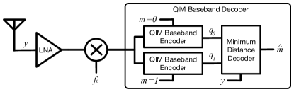
Figure 5: Block diagram of a QIM receiver

II-B QIM Receiver

Fig. 5 shows the block diagram of a QIM receiver. A QIM receiver is based on standard RF architecture and is similar to a commodity receiver in terms of complexity and power consumption. The QIM decoder is implemented in digital baseband and we simply apply the same QIM embedding function to the received signal for both $0$ and $1$ bit messages to obtain two quantized signals $q_{0}$ and $q_{1}$. These are passed through a minimum distance decoder to compare with the original received signal $y$ to obtain estimated/received message,

$$\hat{m}=\arg\min_{m}dist(y,y_{m})$$ (6)

III QIM Techniques

In this section we describe different QIM techniques that can be used to embed messages in a host signal.

III-A Scalar QIM

Scalar QIM is the primary QIM technique which was described in the previous section and can be applied to a real valued or scalar signal.

III-B Distortion Compensated QIM

Distortion compensated QIM (DC-QIM) is an extended version of the QIM method that reduces the distortion in the host signal and significantly improves the distortion to robustness trade-off [8]. The robustness of QIM is a function of the distance between the quantization points. If we increase the distance, robustness of QIM would also increase. This operation is the same as scaling the QIM embedded signal by a factor, $\alpha$. For example, if a sample point $s_{i}$ is shifted to a point, $x$, then by scaling it by $\alpha$, the sample point $s_{i}$ would now be at $\nicefrac{{x}}{{\alpha}}$. However, this increases the distortion of the host signal by a factor $\nicefrac{{1}}{{\alpha^{2}}}$ and results in a $\nicefrac{{\Delta^{2}}}{{12\alpha^{2}}}$ mean distortion. We compensate for the distortion by adding back a fraction, $1-\alpha$ of the host signal. This operation can be represented by the following QIM embedding function,

$$\vspace{-2pt}Q_{m}(\alpha s)=Q(\alpha s-d_{m})+(1-\alpha)s+d_{m}\vspace{-2pt}$$ (7)

The parameter $\alpha$ is defined as $0\leq\alpha\leq 1$ where 1 represents the original QIM method. Since, $\alpha$ determines the distortion, a component of noise in the composite signal due to embedding, we can determine the optimal value of $\alpha$ maximizing the signal to noise ratio $SNR$.

$$SNR(\alpha) =\frac{d_{1}^{2}}{(1-\alpha)^{2}+\alpha^{2}\sigma_{n}^{2}}$$ (8)

$$\frac{\partial SNR(\alpha)}{\partial\alpha} =0\text{ gives }\alpha^{*}=\frac{D_{s}}{D_{s}+\sigma_{n}^{2}},$$

where, $\sigma_{n}^{2}$ is the noise power. Hence, the optimal factor $\alpha^{*}$ is a function of distortion and noise.

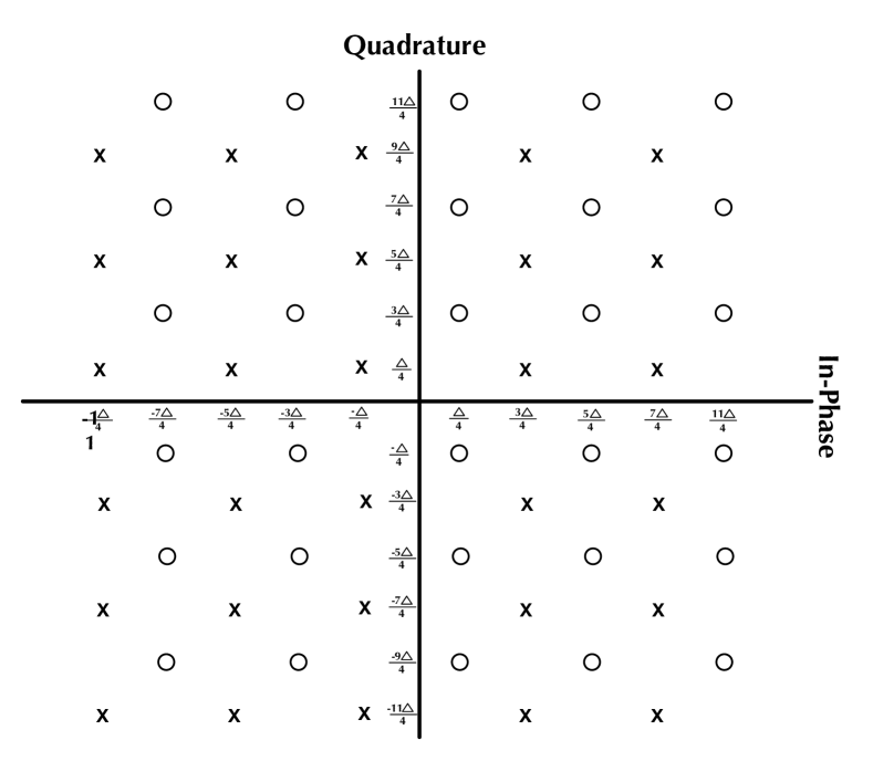
Figure 6: Constellation diagram for Lattice QIM with a grid representation. The Xs are quantization points for 1-bit and Os for a 0-bit.

III-C Lattice QIM

The QIM technique can be extended to higher dimensional signals by using a lattice form [8]. We can arrange the quantization points to be an integer lattice, $Z^{N}$, in an N-dimensional Euclidean space $\textbf{R}^{N}$. Let’s consider a simplified case of a complex or two-dimensional signal which has both in-phase and quadrature phase components. For N=2, we will have two grids to quantize to either a 0-bit or 1-bit representation. As an extension of scalar QIM, the quantization points for a 0-bit and 1-bit can be represented as co-sets of the lattice,

$$\vspace{-2pt}\Lambda_{0}=\big{(}\frac{-\Delta}{4}-j\frac{\Delta}{4}\big{)}+n_{i}\text{ and }\Lambda_{1}=\big{(}\frac{\Delta}{4}+j\frac{\Delta}{4}\big{)}+n_{i}\vspace{-2pt}$$ (9)

where $n_{i}=1,2,...,l$ and $l$ represents the total number of quantization levels. Fig. 6 illustrates the quantization grid for $N=2$. In lattice QIM, the quantization levels are separated by $\nicefrac{{\Delta}}{{2}}$ distance in in-phase and quadrature components resulting in an overall distance of $\nicefrac{{\Delta}}{{\sqrt{2}}}$. However, the mean error due to embedding is still $\frac{\Delta^{2}}{12}$ and because of larger distance between data points, lattice QIM should perform better than scalar QIM. To implement lattice QIM for complex wireless signal, we quantize both the real and imaginary parts of the signal. We use the same embedding function and modify the dither as

$$\vspace{-10pt}\small d_{1}=\frac{\Delta}{4}+j\frac{\Delta}{4}\text{ and }d_{0}=\begin{cases}d_{1}+(\frac{\Delta}{2}+j\frac{\Delta}{2}),&\text{if }d_{1}\leq 0\\ d_{1}-(\frac{\Delta}{2}+j\frac{\Delta}{2}),&\text{otherwise}\end{cases}\vspace{8pt}$$ (10)

Finally, we note that the distortion compensation technique described above can be applied to the real and complex values of the signal to implement distortion compensated lattice QIM.

IV Evaluating the QIM Wireless Link

Evaluation of an embedded communication system (such as QIM) significantly differs from conventional communication systems. Traditional systems deal with only one signal whereas embedded communication systems operate on two signals: the host signal and the embedded signal. We need to evaluate the impact of QIM on the performance of both the host and the embedded message signal: what is the rate and robustness of the embedded signal, and how much did the embedded process distort the host signal and its impact on the output of the host (legacy) receiver.

IV-A Performance of Embedded Message

We start by defining the capacity for QIM embedded message in a Gaussian channel. The output of the channel is the sum of the input host signal and Gaussian white noise. Let $\sigma_{s}^{2}$ be the average power of the host signal and channel noise follows a Gaussian distribution with variance $\sigma_{n}^{2}$. We can express information capacity, i.e., the supremum of the achievable rate for a real value one dimensional signal as [9]

$$C_{host}=\frac{1}{2}\log_{2}\left(1+\frac{\sigma_{s}^{2}}{\sigma_{n}^{2}}\right)$$ (11)

where $\sigma_{s}^{2}/\sigma_{n}^{2}$ denotes the signal-noise ratio (SNR) and assumes that the input also follows Gaussian distribution. Since embedded QIM signal is distortion in the host signal, we can re-write the capacity expression in terms of distortion by treating the embedded QIM signal as a form of power-limited communication over a Gaussian channel:

$$C_{qim}=\frac{1}{2}\log_{2}\left(1+\frac{D_{s}}{\sigma^{2}_{n}}\right)\mathrm{bps/sec/Hz},$$ (12)

where the distortion constraint is given by Eq. 5. The capacity equation, $C_{qim}$, shows that the performance of the embedded message is directly proportional to distortion experienced by the host signal. The QIM technique maximizes the capacity of the embedded message for a given distortion of the host signal. The capacity is also a function of the bandwidth of the host signal and a higher bandwidth host signal would enable a higher data rate embedded message. Finally, we note that the capacity in Eq. 12 is the maximum achievable data rate per unit bandwidth with arbitrarily small error probability. Practical QIM implementation would require error correction coding mechanisms to achieve performance close to the limits promised by channel capacity.

IV-B Impact on the Host Signal

The host signal experiences distortion due to perturbations introduced by the embedded signal which was described in Eq.  5. For a fair comparison across host signals, we introduce normalized distortion which is independent of the signal strength of the host signal and is defined as follows,

$$D_{s}^{n}=\frac{\sum_{i=1}^{N}|s_{i}-x_{i}|^{2}}{\sum_{i=1}^{N}|s_{i}|^{2}}*100\%$$ (13)

Finally, in addition to computing the distortion, we will also analyze the quality of the multimedia signal at the output of the host receiver to ensure that QIM embedding operation has minimal impact on the performance of the host signal.

V Simulation Results

The Wireless QIM technique is independent of the host signal and is universally applicable. Here we consider three host signals: AM, FM and broadcast TV which are ubiquitous in cities. We start with a short primer on the host signals. TV. In the United States, Digital TV (DTV) operates in the UHF band from 470-614 MHz with 6 MHz wide channels and follows the Advanced Television System Committee (ATSC) standard [10]. ATSC uses 8-level vestigial sideband (8-VSB) modulation to transmit data. 8-VSB is a digital modulation technique which uses eight amplitude levels to represent symbols on a 6 MHz channel. Transmissions from a TV tower can be typically received up to 50 miles.

FM Radio. FM radio operates in the 87.8-108 MHz frequency band with 200 kHz wide channels. FM uses analog frequency modulation to encode audio and data i.e. information is transmitted by varying the frequency of the transmitted RF signal. Most FM stations can be heard up to 100 miles from the transmit tower.

AM Radio. In the United States, AM radio operates in the 525-1705 kHz band with 10 kHz channel spacing. AM radio uses amplitude modulation to encode data i.e. information is represented in the amplitude of the signal. AM signals propagate long distances and have been reported to have been received 200 miles away from the station.

We evaluate wireless QIM on recorded AM, FM, and TV signals. The USRP X300 [11] was used to record TV signals centered at 539 MHz (UHF channel 25) with 6.25 MHz sampling rate and FM signal centered at 106.1 MHz with 200kHz sampling rate. We use a WebSDR [12] to record an AM signal centered at 1630 kHz with 8kHz sampling rate. We implement QIM methods described in Section II and simulate different channel conditions and data rates using MATLAB.

We embed pseudo-random message bits and implement scalar QIM and scalar DC-QIM for real valued AM and FM radio signals. For complex TV signals in addition to scalar QIM, we also evaluate lattice QIM and lattice DC-QIM. In DC-QIM, we set $\alpha=0.7$, the optimal value as per Eq. 8. We introduce additive white Gaussian noise to simulate different channel conditions. Finally, a QIM receiver recovers the transmitted message bits using the algorithm described in Section II-B. The value of $\Delta$, the QIM embedding parameter is known at the receiver. This is a reasonable assumption since it can be either pre-set or periodically updated. We evaluate the system by measuring the impact of QIM on both the host signal and the performance of the embedded QIM signal for different QIM methods at different channel conditions and number of quantization levels (affects distortion).

V-A Impact on the Host Signal

The distortion experienced by the host signal is a function of number of levels $N$ used in the QIM embedding process. We vary the number of quantization levels from 2 to 45 for embedding random messages in TV, FM and AM host signals and measure the normalized distortion and its impact on the performance of the legacy host signal receiver.

Figure 7: Evaluation of distortion for each host signal

Normalized Distortion. Fig. 7 shows the percentage of distortion experienced by each host signal as a function of number of levels for scalar DC-QIM technique. The AM signal experiences the most distortion followed by TV and FM. This is expected since AM uses analog amplitude modulation to encode data and QIM introduces amplitude perturbations, which distorts the information carrying amplitude of the AM signal. Similarly, TV also uses 8 level (digital) amplitude modulation and amplitude perturbations would impact the digital TV signal but since digital amplitude modulation is more robust compared to analog modulation, QIM introduces less distortion in case of TV compared to AM.

The FM signal is the most robust among evaluated signals with less than 8% for four quantization levels since amplitude perturbations introduced by QIM have minimal impact on the frequency modulated FM signal.

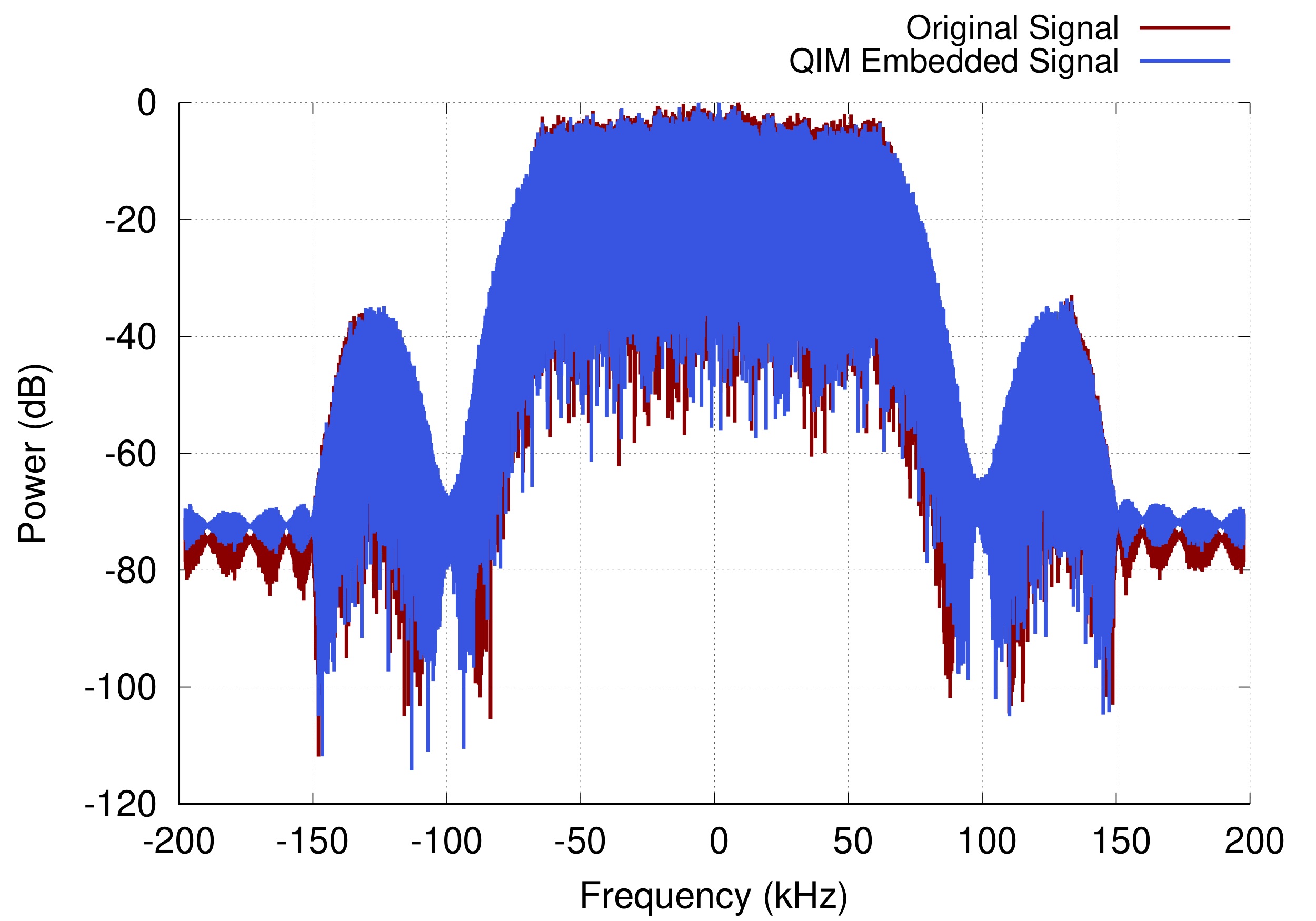
Figure 8: Spectrum of the baseband FM signal before and after QIM embedded data.

Distortion in the Frequency Domain. Next, we evaluate impact of embedding data using QIM in the frequency domain. Fig. 8 shows the spectrum of the baseband FM signal before and after the QIM embedding process. The two signals are passed through pulse shaping low pass filters to comply with spectral mask requirements. Our results show that there is small distortion in the in-band spectral characteristics of the baseband signal which corroborate the time domain distortion analysis. The out of band frequency components for both before and after QIM embedded baseband FM signal are atleast 35 dB below the main lobe thereby having minimal impact on any side channels.

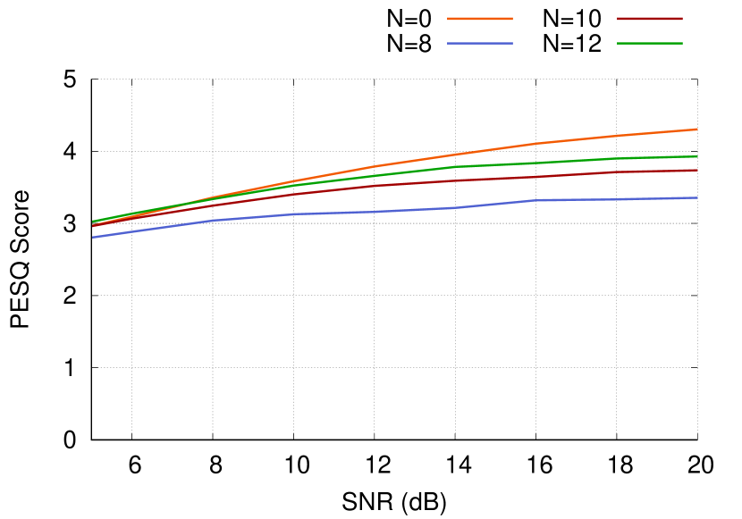
(a) Quality of AM audio.

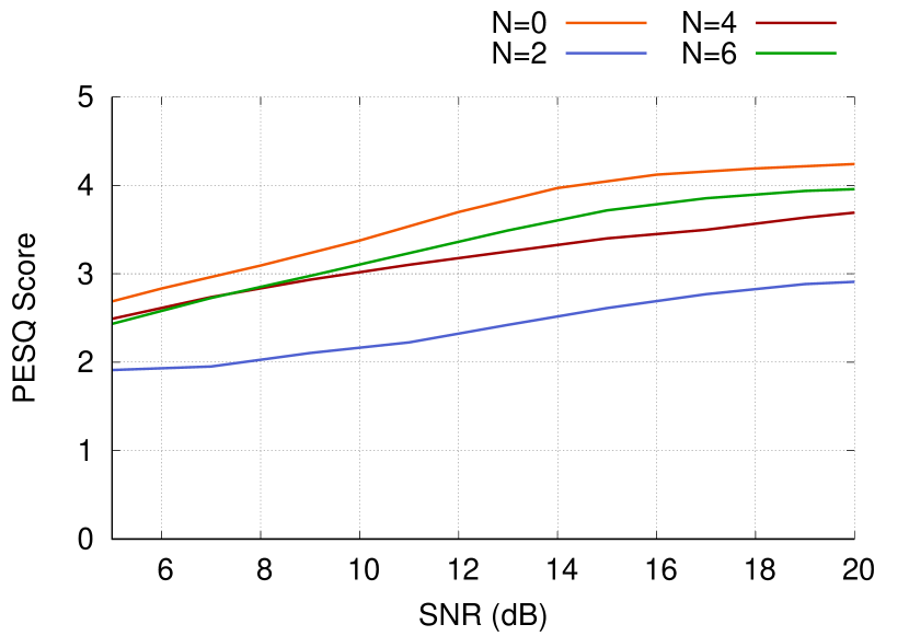
(b) Quality of FM audio.

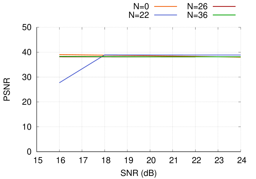
(c) Quality of TV video.

Figure 9: Evaluation of the quality of the host signal multimedia after QIM embedding.

Impact on Host Signal Multimedia. The next step is to translate the distortion to the quality of the multimedia audio and video signal carried by AM, FM and TV signals. This is the key to understanding how QIM impacts the information carried by the host signal. We use the Perceptual Evaluation of Speech Quality (PESQ) metric to quantify the quality of demodulated audio from AM and FM signals. The results model a mean opinion score (MOS) that ranks the quality of speech from 1(bad) to 5(excellent). As a reference, a PESQ $\geq$ 1 is sufficient for human hearing [13]. We evaluate the PESQ as function of the SNR of the host signal and distortion introduced by scalar DC-QIM technique. Fig. 9(a) shows the audio quality of an AM signal as a function of SNR of the host signal and the number of quantization levels. We can see that even at the lowest SNR of 6 dB, PESQ is greater than 2.8 which is sufficient for most applications. As we increase the SNR and number of quantization levels, the audio quality improves. The results confirm that QIM has minimal impact on the audio quality of AM signals. We perform similar analysis for FM signal and Fig. 9(b) shows the audio quality of a demodulated QIM embedded FM signal at different host signal SNR and quantization levels. Since the FM signal is more robust to QIM, we evaluate the scalar DC-QIM technique for 2-6 quantization levels (42$\%$-2$\%$ distortion) in the FM baseband. However, due to the robustness of frequency modulation, even at the worst-case SNR of 6 dB and 42$\%$ distortion, PESQ is close to 2, which is satisfactory.

Finally, we evaluate the video quality of the QIM embedded TV signal, using the peak SNR (PSNR) metric which is the ratio of maximum possible power of a signal to the power of the distorting noise [14]. The PSNR is computed as follows

$$PSNR=10log_{10}(\frac{(max(s))^{2}}{D_{s}})$$ (14)

where $D_{s}$ is distortion defined in Eq. 5. For typical applications, PSNR values between 20-25 dB are acceptable for wireless systems [14].

To evaluate the PSNR of the video signal, we first extract the video by demodulating the QIM embedded TV host signal. We use a software defined radio (USRP X300) to re-transmit the QIM embedded TV signal at different SNR to a TV tuner card by Hauppauge to recover the video. The TV signal was embedded with 20-36 quantization levels which translates to 0.9%–0.3% distortion in the TV baseband signal. In Fig. 9(c) we plot the PSNR of the video output of the TV tuner card as a function of SNR of the host TV signal and number of levels. The PSNR of the recovered video was around 34 for majority of the cases expect for the lowest SNR of 16 dB at the highest distortion. However, even the lowest values of 28 dB PSNR is acceptable for most applications. Our analysis considers TV signals above an SNR of 16 dB, a constraint placed by the sensitivity of the TV tuner card. The TV tuner was only able to play video from original distortion free TV signal above an SNR of 16 dB which placed the limit on the SNR of the TV signal evaluated in this work.

To give readers an intuition about the quality metric used in the evaluation, we created a composite video of audio and video clips for AM, FM and TV host signals for different SNR and distortion in the host signal which can be found at the following web link:

https://youtu.be/gKn09ctlFMA.

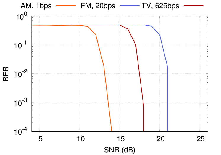
Figure 10: A comparison of performance of all three host signals.

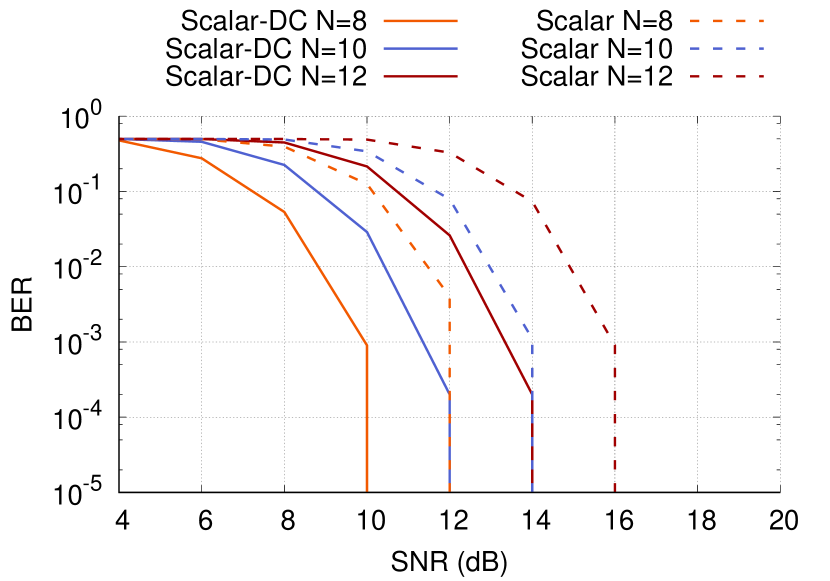
(a) Scalar and Scalar-DC QIM on AM signal.

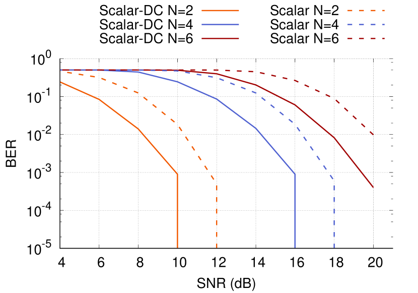
(b) Scalar and Scalar-DC QIM on FM signal.

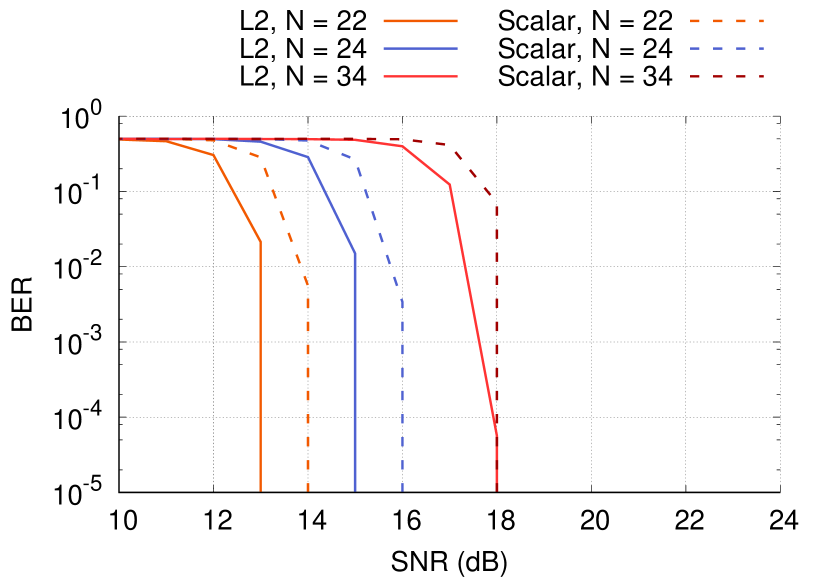
(c) Scalar-DC and Lattice-DC QIM on TV signal.

Figure 11: We evaluate the performance of embedding message using QIM on each of the three host signals.

V-B Performance of the QIM Embedded Message

The next step is to evaluate the performance of the QIM embedded message signal. We only consider scenarios where the distortion and impact on the host multimedia is within acceptable bounds described in Section  V-A.

In Section IV we showed that the information carrying capacity of QIM, like any communication system, is directly proportional to the bandwidth of the host signal. To have a fair comparison across different signals, we normalize the embedded message data rate to the bandwidth of the host signal and evaluate performance for all three host signals. Specifically, we embed at the rate of 1 bps for 10 kHz bandwidth AM signal, 20 bps for 200 kHz bandwidth FM signal and 625 bps for 6.25 MHz bandwidth TV signal. Fig. 10 shows the BER of the embedded message using 22 level scalar DC-QIM for the three host signals which translates to 1%, 0.3% and 0.7% distortion respectively in the AM, FM and TV signals. We can see that there is a 4 dB difference between AM and TV and a 7 dB difference between AM and FM. This can be attributed to the fact that for the same number of levels, the AM signal experiences 0.35% more distortion compared to TV and 0.76% more distortion compared to FM. Since distortion is the embedded signal, a higher distortion translates to higher signal strength for the embedded message signal and better performance. We empirically note an approximate 1 dB increase in performance for every 0.1$\%$ increase in distortion.

Next, we individually analyze each of the three host signals by evaluating the BER of embedded message as a function of the SNR of the host signal and the signal strength of the embedded message. We evaluate the AM signal for 8-16 levels at 200bps embedded message rate for both scalar QIM and scalar DC QIM. Fig. 11(a) shows that the BER decreases with decrease in number of levels which translates to an increase in distortion of the host signal or signal strength of the embedded signal. Specifically, for every decrease in two quantization levels, there is a 2 dB increase in the performance. Finally, the distortion compensation technique improves the performance by about 2 dB and this is true for all host signals and both scalar and lattice DC-QIM methods.

For the distortion tolerant FM signals we embed message at 20 kbps and use 2–6 quantization levels which translates to a distortion of 42% to 4%. Fig. 11(b) shows the performance of scalar and scalar DC QIM for the host FM signal. We observe a 2 dB increase in performance for every unit decrease in number of quantization levels.

Finally, we evaluate the TV signal for both scalar and lattice DC-QIM techniques. Since TV signals are susceptible to distortion, we embed messages at 250 bps and use 22–48 quantization levels which translates to a distortion of 0.7% to 0.1% in the host TV signal. Fig. 11(c) plots the performance of an embedded QIM message in a host TV signal and we can see that performance increase with decrease in number of levels or increase in distortion. Additionally, lattice DC-QIM outperforms scalar DC-QIM by about 2 dB.

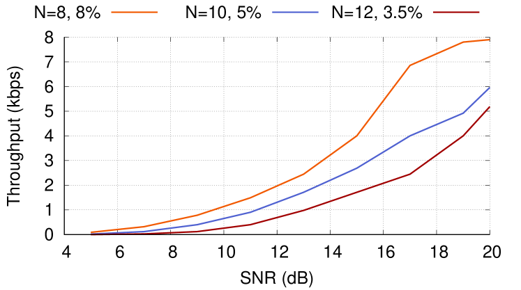
(a) Achievable throughput with low distortion in host signal (AM signal).

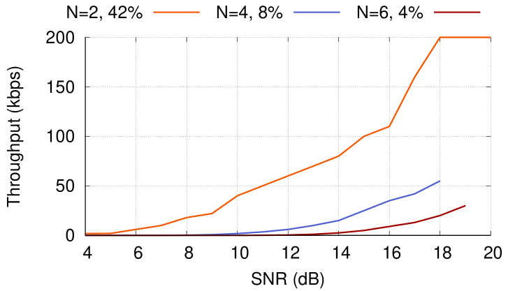
(b) Achievable throughput with high distortion in host signal (FM signal).

Figure 12: We evaluate the achievable throughput using Scalar-DC QIM with high and low distortion in host signals.

V-C Achievable Throughput

We analyze achievable throughput for high and low distortion in the host signal. For low distortion in a host signal, we consider the 10 kHz wide AM radio signal and embed messages using scalar DC-QIM method at different data rates using 8–16 quantization levels (8%–3.5% distortion). Fig. 12(a) shows the throughput as a function of SNR for different quantization levels. We can see that QIM embedded message achieves the maximum throughput of 8 kbps for SNR of 20 dB for 8 quantization levels (8% distortion). Every decrement in two quantization levels increases the throughput by a factor of 1.5 and every 2 dB increase in SNR increase the throughput by an average factor of 3. We can scale these results for FM and TV signals by respectively multiplying the AM data rates by 20 and 625. For a high distortion case, we consider the 200 kHz wide FM radio signal and embed messages using scalar DC-QIM method with 2–6 quantization levels (42%–4% distortion). We plot throughput as a function of SNR for different quantization levels in Fig. 12(b). We achieve a maximum throughput of 200 kbps.

VI Related Work

Our work is related to recent efforts in spread spectrum watermarking of RF signals [15]. Spread spectrum is a promising technique because it is robust against interfering noise. However, it is a linear method and is susceptible to host signal interference. On the other hand, QIM is a non-linear techniques which is aware of the host signal and therefore efficiently manages host signal interference, resulting in better overall performance. Wireless QIM is also related to inter-protocol communication techniques which enable communication between IoT devices using different wireless standards. This is especially beneficial in the crowded 2.4GHz spectrum where devices with a software modification can using existing hardware to communicate between different devices employing different standards. For instance, the WiZip system uses the presence and absence of packets to encode information for transmission from a Wi-Fi device to a ZigBee device [16]. FreeBee uses variance in timing of regular Wi-Fi beacons to transmit information to ZigBee devices [17]. $B^{2}W^{2}$ uses presence and absence of packets to enable BLE to Wi-Fi communication while concurrently supporting existing Wi-Fi and BLE communication [18].

All of these techniques are promising, but they are limited to low data rates, are short range and spectrally inefficient since Wi-Fi and ZigBee use drastically different bandwidths. Instead, the Wireless QIM technique can achieve data rates up to 8 kbps with only a 10 kHz wide host AM signal which is 52, 470, and 5.5 order of magnitude higher when compared to WiZig, FreeBee, and $B^{2}W^{2}$ which use a significantly wider bandwidth (20 MHz) signal.

VII Conclusion and Future Work

We have introduced Wireless QIM technique to embed information into existing signals and communicate with smart devices while having negligible impact on the host signal. We have demonstrated communication at up to of 8 kbps for low bandwidth distortion sensitive AM signals and 200 kbps for higher bandwidth, but distortion resilient FM signals. To the best of our knowledge, this is the first work to use QIM technique to embed messages into wireless signals. We believe Wireless QIM presents a new and exciting opportunity for the radio/TV/cellular providers to enable smart cities and IoT applications by reusing their existing infrastructure and deliver additional value with connectivity at zero spectrum overhead.

In this paper, although we have evaluated data rate and reliability of the embedded message, we haven’t explored errors correcting codes. Development of error correcting codes for Wireless QIM to achieve data rates closer to the theoretical capacity of the channel is an exciting avenue for future research. Finally, this work was focused on downlink communication and in the future work we will extend the Wireless QIM technique for uplink communication as well.

VIII Acknowledgements

This work is supported in part by NSF award CNS-1305072 and a Google faculty research award.

References

- [1] Gartner, “http://www.gartner.com/newsroom/id/2636073.”
- [2] R. Musaloiu-E and A. Terzis, “Minimising the effect of wifi interference in 802.15. 4 wireless sensor networks,” International Journal of Sensor Networks, vol. 3, no. 1, pp. 43–54, 2008.
- [3] S. Gollakota et al., “Clearing the rf smog,” in Proceedings of the ACM Special Interest Group on Data Communication (SIGCOMM). Association for Computing Machinery, 2011.
- [4] L. Technology, “https://www.lora-alliance.org/what-islora/technology.”
- [5] SIGFOX, “https://www.lora-alliance.org/what-islora/technology.”
- [6] P. Bahl, R. Chandra, T. Moscibroda, R. Murty, and M. Welsh, “White space networking with wi-fi like connectivity,” in Proceedings of the ACM SIGCOMM 2009 Conference on Data Communication, ser. SIGCOMM ’09. New York, NY, USA: ACM, 2009, pp. 27–38. [Online]. Available: http://doi.acm.org/10.1145/1592568.1592573
- [7] FCC, “https://ecfsapi.fcc.gov/file/6518909731.pdf.”
- [8] B. Chen and G. Wornell, “Quantization index modulation: a class of provably good methods for digital watermarking and information embedding,” in IEEE TRANSACTION ON INFORMATION THEORY, 2001.
- [9] T. M. Cover and J. A. Thomas, Elements of Information Theory.
- [10] A. T. S. Committee, “https://www.atsc.org/.”
- [11] E. Research, “https://www.ettus.com/product/details/x300-kit.”
- [12] WebSDR, “http://www.websdr.org.”
- [13] Y. Hu and P. C. Loizou, “Evaluation of objective quality measures for speech enhancement,” IEEE Transactions on Audio, Speech, and Language Processing, vol. 16, no. 1, pp. 229–238, Jan 2008.
- [14] N. Thomos, N. V. Boulgouris, and M. G. Strintzis, “Optimized transmission of jpeg2000 streams over wireless channels,” IEEE Transactions on Image Processing, vol. 15, no. 1, pp. 54–67, Jan 2006.
- [15] X. Xie, Z. Xu, and H. Xie, “Channel capacity analysis of spread spectrum watermarking in radio frequency signals,” IEEE Access, vol. PP, no. 99, pp. 1–1, 2017.
- [16] X. Guo, X. Zheng, and H. Yuan, “Wizig: Cross-technology energy communication over a noisy channel,” in The 36th Annual IEEE International Conference on Computer Communications (INFOCOM), 2017.
- [17] S. M. Kim and T. He, “Freebee: Cross-technology communication via free side-channel,” in Proceedings of the 21st Annual International Conference on Mobile Computing and Networking, ser. MobiCom ’15. New York, NY, USA: ACM, 2015, pp. 317–330. [Online]. Available: http://doi.acm.org/10.1145/2789168.2790098
- [18] Z. Chi, Y. Li, H. Sun, Y. Yao, Z. Lu, and T. Zhu, “B2w2: N-way concurrent communication for iot devices,” in Proceedings of the 14th ACM Conference on Embedded Network Sensor Systems CD-ROM, ser. SenSys ’16. New York, NY, USA: ACM, 2016, pp. 245–258. [Online]. Available: http://doi.acm.org/10.1145/2994551.2994561