Experimental Classification of Entanglement in Arbitrary Three-Qubit States on an NMR Quantum Information Processor

Abstract

We undertake experimental detection of the entanglement present in arbitrary three-qubit pure quantum states on an NMR quantum information processor. Measurements of only four observables suffice to experimentally differentiate between the six classes of states which are inequivalent under stochastic local operation and classical communication (SLOCC). The experimental realization is achieved by mapping the desired observables onto Pauli $z$-operators of a single qubit, which is directly amenable to measurement. The detection scheme is applied to known entangled states as well as to states randomly generated using a generic scheme that can construct all possible three-qubit states. The results are substantiated via direct full quantum state tomography as well as via negativity calculations and the comparison suggests that the protocol is indeed successful in detecting tripartite entanglement without requiring any a priori information about the states.

I Introduction

Quantum entanglement plays a fundamental role in quantum information processing and is a key resource for several quantum computational and quantum communication tasks Horodecki et al. (2009). Any experiment aimed at entanglement generation needs as an integral part, a way to establish that entanglement has indeed been generated Gühne and Tóth (2009). Therefore, the detection of entanglement and its characterization is a foundational problem and is a key focus of research in quantum information processing Li et al. (2013). Entanglement detection and certification protocols include quantum states tomography Thew et al. (2002), entanglement witness operators Gühne et al. (2003); Arrazola et al. (2012); Jungnitsch et al. (2011), of the density operator under partial transposition Peres (1996); Li et al. (2017) and the violation of Bell’s inequalities DiVincenzo and Peres (1997).

Experimentally, entanglement has been created in various physical systems including nitrogen-vacancy defect centers (Neumann et al., 2008), trapped-ion quantum computers (Mandel et al., 2003), superconducting phase qubits (Neeley et al., 2010) nuclear spin qubits (Dogra et al., 2015) and quantum dots (Gao et al., 2012). Bound entanglement was created and detected using three nuclear spins Kampermann et al. (2010) and there have been several efforts to create and detect three-qubit entanglement using NMR Laflamme et al. (1998); Peng et al. (2010); Rao and Kumar (2012); Das et al. (2015); Xin et al. (2018). Witness based entanglement detection protocols have been implemented experimentally in quantum optics (Bourennane et al., 2004) and NMR (Filgueiras et al., 2012). Concurrence (Wootters, 2001) was measured by a single measurement on twin copies of the quantum state of photons (Walborn et al., 2006) while entanglement of formation was used as an entanglement quantifier in four trapped ions (Sackett et al., 2000). While there have been various experimental advances to detect entanglement yet characterizing entanglement experimentally as well as computationally is a daunting task Dür and Cirac (2001); Altepeter et al. (2005); Spengler et al. (2012); Dai et al. (2014). Therefore it is desirable to invent and implement protocols to certify the existence of entanglement which are not intensive on resources.

In the present study we undertake the experimental characterization of arbitrary three-qubit pure states. The three-qubit states can be classified into six inequivalent classes Dür et al. (2000) under SLOCC (Bennett et al., 2000).Protocols have been invented to carry out the classification of three-qubit states into the SLOCC classes Chi et al. (2010); Zhao et al. (2013). A recent proposal aims to classify any three-qubit pure entangled state into these six inequivalent classes by measuring only four observables (Adhikari et al., 2017). We have previously constructed a scheme to experimentally realize a canonical form for general three-qubit states, which we use here to prepare arbitrary three-qubit states with an unknown amount of entanglement. Experimental implementation of the entanglement detection protocol is such that in a single shot (using only four experimental settings), we were able to determine if a state belongs to the $\rm W$ class or to the ${\rm GHZ}$ class. We use our own scheme to map the desired observables onto the $z$-magnetization of one of the subsystems, making it possible to experimentally measure its expectation value on NMR systems (Singh et al., 2016). Mapping of the observables onto Pauli $z$-operators of a single qubit eases the experimental determination of the desired expectation value, since the NMR signal is proportional to the ensemble average of the Pauli $z$-operator.

We implement the protocol on known three-qubit entangled states such as the ${\rm GHZ}$ state and the $W$ state and also implement it on randomly generated arbitrary three-qubit states with an unknown amount of entanglement. Seven representative states belonging to the six SLOCC inequivalent classes as well as twenty random states were prepared experimentally, with state fidelities ranging between 89% to 99%. To decide the entanglement class of a state, the expectation values of four observables were experimentally measured in the state under investigation. All the seven representative states (namely, GHZ, W, $\rm W\overline{W}$, three bi-separable states and a separable state) were successfully detected within the experimental error limits. Using this protocol, the experimentally randomly generated arbitrary three-qubit states were correctly identified as belonging to either the GHZ, the W, the bi-separable or the separable class of states. We also perform full quantum state tomography to directly compute the observable value. Reconstructed density matrices were used to calculate the entanglement by computing negativity in each case, and the results compared well with those of the current protocol.

The paper is organized as follows: Section II briefly describes the theoretical framework, while the mapping of the required observables onto single-qubit $z$ magnetization is discussed in Section II.1. Section III presents the experimental implementation of the entanglement characterization protocol on a three-qubit NMR quantum information processor. Section IV contains some concluding remarks.

II Detecting Tripartite Entanglement

There are six SLOCC inequivalent classes of entanglement in three-qubit systems, namely, the GHZ, W, three different biseparable classes and the separable class Dür et al. (2000). A widely used measure of entanglement is the $n$-tangle Wong and Christensen (2001); Li (2012) and a non-vanishing three-tangle is a signature of the GHZ entangled class and can hence be used for their detection. For three parties A, B and C, the three-tangle $\tau$ is defined as

$$\tau=C^{2}_{\rm{A(BC)}}-C^{2}_{\rm{AB}}-C^{2}_{\rm{AC}}$$ (1)

with $C_{\rm{AB}}$ and $C_{\rm{AC}}$ being the concurrence that characterizes entanglement between A and B, and between A and C respectively; $C_{\rm{A(BC)}}$ denotes the concurrence between A and the joint state of the subsystem comprising B and C Coffman et al. (2000).

The idea of using the three-tangle to investigate entanglement in three-qubit generic states is particularly interesting and general, as any three-qubit pure state can be written in the canonical form Acín et al. (2001)

$$|\psi\rangle=a_{0}|000\rangle+a_{1}e^{\iota\theta}|100\rangle+a_{2}|101\rangle+a_{3}|110\rangle+a_{4}|111\rangle$$ (2)

where $a_{i}\geq 0$, $\sum_{i}a^{2}_{i}=1$ and $\theta\in[0,\pi]$, and the class of states is written in the computational basis $\{|0\rangle,|1\rangle\}$ of the qubits. The three-tangle for the generic state given in Eq. 2 turns out to be (Adhikari et al., 2017)

$$\tau_{\psi}=4a^{2}_{0}a^{2}_{4}$$ (3)

Three-tangle can be measured experimentally by measuring the expectation value of the operator $O=2\sigma_{1x}\sigma_{2x}\sigma_{3x}$, in the three qubit state $|\psi\rangle$. Here $\sigma_{x,y,z}$ are the Pauli matrices and $i=1,2,3$ denotes qubits label and the tensor product symbol between the Pauli operators has been omitted for brevity. Since, $\langle\psi|O|\psi\rangle^{2}=\langle O\rangle^{2}_{\psi}=4\tau_{\psi}$, a non-zero expectation value of $O$ implies that the state under investigation is in the GHZ class (Dür et al., 2000). In order to further categorize the classes of three-qubit generic states we need three more observables $O_{1}=2\sigma_{1x}\sigma_{2x}\sigma_{3z}$, $O_{2}=2\sigma_{1x}\sigma_{2z}\sigma_{3x}$, $O_{3}=2\sigma_{1z}\sigma_{2x}\sigma_{3x}$. Experimentally measuring the expectation values of the operators $O$, $O_{1}$, $O_{2}$ and $O_{3}$ can reveal the entanglement class of every three-qubit pure state Zhao et al. (2013); Adhikari et al. (2017). Table 1 summarizes the classification of the six SLOCC inequivalent classes of entangled states based on the expectation values of the observables $O$, $O_{1}$, $O_{2}$, $O_{3}$.

Table 1: Decision table for the classification of three qubit pure entangled states based on the expectation values of operators $O$, $O_{1}$, $O_{2}$ and $O_{3}$ in state $|\psi\rangle$. Each class in the row is shown with the expected values of the observables.

Class	$\langle O\rangle$	$\langle O_{1}\rangle$	$\langle O_{2}\rangle$	$\langle O_{3}\rangle$
GHZ	$\neq 0$	$*$	$*$	$*$
W	0	$\neq 0$	$\neq 0$	$\neq 0$
BS1	0	0	0	$\neq 0$
BS2	0	0	$\neq 0$	0
BS3	0	$\neq 0$	0	0
Separable	0	0	0	0

$*$ May or may not be zero.

The six SLOCC inequivalent classes of three-qubit entangled states are GHZ, W, BS₁, BS₂, BS₃ and separable. While GHZ and W classes are well known, BS₁ denotes a biseparable class having B and C subsystems entangled, the BS₂ class has subsystems A and C entangled, while the BS₃ class has subsystems A and B entangled. As has been summarized in Table 1 a non-zero value of $\langle O\rangle$ indicates that the state is in the GHZ class and this expectation value is zero for all other classes. For the W class of states all $\langle O_{j}\rangle$ are non-zero except $\langle O\rangle$. For the BS₁ class only $\langle O_{3}\rangle$ is non-zero while only $\langle O_{2}\rangle$, and $\langle O_{1}\rangle$ are non-zero for the classes BS₂ and BS₃, respectively. For separable states all expectations are zero.

In order to experimentally realize the entanglement characterization protocol, one has to determine the expectation values $\langle O\rangle$, $\langle O_{1}\rangle$, $\langle O_{2}\rangle$ and $\langle O_{3}\rangle$ for an experimentally prepared state $|\psi\rangle$. In the next section we will describe our method to experimentally realize these expectation values based on subsystem measurement of the Pauli $z$-operator Singh et al. (2016) and our experimental scheme for generating arbitrary 3 qubit states Dogra et al. (2015).

II.1 Mapping Pauli basis operators to single qubit $z$-operators

A standard way to determine the expectation value of a desired observable in an experiment is to decompose the observable as a linear superposition of the observables accessible in the experiment Nielsen and Chuang (2000). This task becomes particularly accessible while dealing with the Pauli basis.

Any observable for a three-qubit system, acting on an eight-dimensional Hilbert space can be decomposed as a linear superposition of 64 basis operators, and the Pauli basis is one possible basis for this decomposition. Let the set of Pauli basis operators be denoted as $\mathbb{B}=\{\rm{B}_{i};0\leq i\leq 63\}$. For example, $O_{2}$ has the form $\sigma_{1x}\sigma_{2z}\sigma_{3x}$ and it is the element B₂₉ of the basis set $\mathbb{B}$. The four observables $O$, $O_{1}$, $O_{2}$ and $O_{3}$ are represented by the elements B₂₁, B₂₃, B₂₉ and B₅₃ respectively of the Pauli basis set $\mathbb{B}$. Also by this convention the single-qubit $z$-operators for the first, second and third qubit i.e. $\sigma_{1z}$, $\sigma_{2z}$ and $\sigma_{3z}$ are the elements B₄₈, B₁₂ and B₃ respectively.

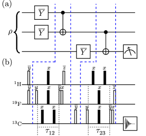
Figure 1: (a) Quantum circuit to achieve mapping of the state $\rho$ to either of the states $\rho_{21}$, $\rho_{23}$, $\rho_{29}$ or $\rho_{53}$ followed by measurement of qubit 3 in the computational basis. (b) NMR pulse sequence of the quantum circuit given in (a). All the unfilled rectangles denote $\frac{\pi}{2}$ spin-selective RF pulses while filled rectangles denote $\pi$ pulses. Pulse phases are written above the respective pulse and a bar over a phase represents negative phase. Delays are given by $\tau_{ij}=1/(8J_{ij})$; $i,j$ label the qubit and $J$ is the coupling constant.

Table 4 in Appendix A details the mapping of all 63 Pauli basis operators (excluding the 8$\otimes$8 identity operator) to the single-qubit Pauli $z$-operator. This mapping is particularly useful in an experimental setup where the expectation values of Pauli’s local $z$-operators are easily accessible. In NMR experiments, the $z$-magnetization of a nuclear spin in a state is proportional to the expectation value of Pauli $z$-operator of that spin in the state.

As an example of the mapping given in Table 4, the operator $O_{2}$ has the form $\sigma_{1x}\sigma_{2z}\sigma_{3x}$ and is the element B₂₉ of basis set $\mathbb{B}$. In order to determine $\langle O_{2}\rangle$ in the state $\rho=|\psi\rangle\langle\psi|$, one can map the state $\rho\rightarrow\rho_{29}=U_{29}.\rho.U^{\dagger}_{29}$ with $U_{29}={\rm CNOT}_{23}.\overline{Y}_{3}.{\rm CNOT}_{12}.\overline{Y}_{1}$. This is followed by finding $\langle\sigma_{3z}\rangle$ in the state $\rho_{29}$. The expectation value $\langle\sigma_{3z}\rangle$ in the state $\rho_{29}$ is equivalent to the expectation value of $\langle O_{2}\rangle$ in the state $\rho=|\psi\rangle\langle\psi|$(Table 4); the operation ${\rm CNOT}_{kl}$ is a controlled-NOT gate with $k$ as the control qubit and $l$ as the target qubit, and $X$, $\overline{X}$, $Y$ and $\overline{Y}$ represent local $\frac{\pi}{2}$ unitary rotations with phases $x$, $-x$, $y$ and $-y$ respectively. The subscript on $\pi/2$ local unitary rotations denotes qubit number. The quantum circuit to achieve such a mapping is shown in Fig. 1(a).

It should be noted that while measuring the expectation values of $O$, $O_{1}$, $O_{2}$ or $O_{3}$, all the $\overline{Y}$ local rotations may not act in all these four cases. The mapping given in Table 4 is used to decide which $\overline{Y}$ local rotation in the circuit 1(a) will act. All the basis operators in set $\mathbb{B}$ can be mapped to single qubit $z$-operators in a similar fashion. The mapping given in Table 4 is not unique and there are several equivalent mappings which can be worked out as per the experimental requirements.

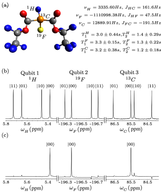
Figure 2: (a) Molecular structure of ${}^{13}C$-labeled diethyl fluoromalonate and NMR parameters. NMR spectra of (b) thermal equilibrium state (c) pseudopure state. Each peak is labeled with the logical state of the qubit which is passive during the transition. Horizontal scale represents the chemical shifts in ppm.

III NMR Implementation of Three Qubit Entanglement Detection Protocol

The Hamiltonian (Ernst et al., 1990) for a three-qubit system in the rotating frame is given by

$$\mathcal{H}=-\sum_{i=1}^{3}\nu_{i}I_{iz}+\sum_{i>j,i=1}^{3}J_{ij}I_{iz}I_{jz}$$ (4)

where the indices $i,j=$ 1,2 or 3 represent the qubit number and $\nu_{i}$ is the respective chemical shift in rotating frame, $J_{ij}$ is the scalar coupling constant and $I_{iz}$ is the Pauli’s $z$-spin angular momentum operator of the $i^{\rm{th}}$ qubit. To implement the entanglement detection protocol experimentally, ¹³C labeled diethyl fluoromalonate dissolved in acetone-D6 sample was used. ¹H, ¹⁹F and ¹³C spin-half nuclei were encoded as qubit 1, qubit 2 and qubit 3 respectively. The system was initialized in the pseudopure (PPS) state i.e. $|000\rangle$ using the spatial averaging Cory et al. (1998); Mitra et al. (2007) with the density operator being

$$\rho_{000}=\frac{1-\epsilon}{2^{3}}\mathbb{I}_{8}+\epsilon|000\rangle\langle 000|$$ (5)

where $\epsilon\sim 10^{-5}$ is the thermal polarization at room temperature and $\mathbb{I}_{8}$ is the 8 $\times$ 8 identity operator. The experimentally determined NMR parameters (chemical shifts, T₁ and T₂ relaxation times and scalar couplings $\rm{J}_{ij}$) as well as the NMR spectra of the PPS state are shown in Fig. 2. Each spectral transition is labeled with the logical states of the passive qubits (i.e. qubits not undergoing any transition) in the computational basis. The state fidelity of the experimentally prepared PPS (Fig. 2(c)) was compute to be 0.98$\pm$0.01 and was calculated using the fidelity measure (Uhlmann, 1976; Jozsa, 1994)

$$F=\left[Tr\left(\sqrt{\sqrt{\rho_{{\rm th}}}\rho_{{\rm ex}}\sqrt{\rho_{{\rm th}}}}\right)\right]^{2}$$ (6)

where $\rho_{{\rm th}}$ and $\rho_{{\rm ex}}$ are the theoretically expected and the experimentally reconstructed density operators, respectively. Fidelity measure is normalized such that $F\rightarrow 1$ as $\rho_{ex}\rightarrow\rho_{th}$. For the experimental reconstruction of density operator, full quantum state tomography (QST)(Leskowitz and Mueller, 2004; Singh et al., 2016) was performed using a preparatory pulse set $\left\{III,XXX,IIY,XYX,YII,XXY,IYY\right\}$, where $I$ implies “no operation”. In NMR a $\frac{\pi}{2}$ local unitary rotation $X$($Y$) can be achieved using spin-selective transverse radio frequency (RF) pulses having phase $x$($y$).

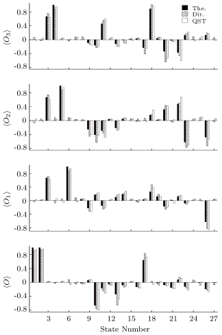
Figure 3: Bar plots of the expectation values of the observables $O$, $O_{1}$, $O_{2}$ and $O_{3}$ for states numbered from 1-27 (Table 2). The horizontal axes denote the state number while the vertical axes represent the values of the respective observable. Black, cross-hatched and unfilled bars represent the theoretical (The.), directly (Dir.) measured from experiment, and QST-derived expectation values, respectively.

Table 2: Results of the three qubit entanglement detection protocol for twenty seven states. Label BS is for biseparable states while R is for random states. First column depicts the state label, top row lists the observable (Obs.) while second row specify if the observable value is theoretical (The.), direct experimental (Dir.) or from QST.

Obs. $\rightarrow$	$\langle O\rangle$			$\langle O_{1}\rangle$			$\langle O_{2}\rangle$			$\langle O_{3}\rangle$
State($F$) $\downarrow$	The.	Dir.	QST	The.	Dir.	QST	The.	Dir.	QST	The.	Dir.	QST
GHZ(0.95 $\pm$ 0.03)	1.00	0.91	0.95	0	-0.04	0.03	0	-0.07	0.05	0	0.07	-0.02
$\rm W\overline{W}$(0.98 $\pm$ 0.01)	1.00	0.94	0.96	0	0.02	0.03	0	0.05	-0.02	0	-0.03	0.05
W(0.96 $\pm$ 0.02)	0	0.05	0.04	0.67	0.60	0.62	0.67	0.61	0.69	0.67	0.59	0.63
BS1(0.95 $\pm$ 0.02)	0	-0.03	0.02	0	-0.07	0.06	0	0.09	0.03	1.00	0.93	0.95
BS2(0.96 $\pm$ 0.03)	0	0.04	0.04	0	0.06	-0.05	1.00	0.90	0.95	0	0.05	0.05
BS3(0.95 $\pm$ 0.04)	0	0.08	-0.06	1.00	0.89	0.94	0	0.09	0.07	0	-0.04	0.02
Sep(0.98 $\pm$ 0.01)	0	-0.05	0.02	0	0.09	-0.04	0	0.04	0.03	0	0.08	0.07
R1 ( 0.91 $\pm$ 0.02 )	-0.02	-0.05	-0.05	0.04	0.06	0.05	0.00	0.03	0.01	0.00	0.09	0.03
R2 ( 0.94 $\pm$ 0.03 )	0.06	0.09	0.08	-0.22	-0.32	-0.33	-0.25	-0.46	-0.41	-0.09	-0.13	-0.16
R3 ( 0.93 $\pm$ 0.03 )	-0.66	-0.76	-0.80	0.17	0.19	0.23	-0.41	-0.63	-0.42	-0.16	-0.23	-0.20
R4 ( 0.91 $\pm$ 0.01 )	-0.17	-0.25	-0.31	-0.15	-0.25	-0.21	-0.29	-0.37	-0.48	0.46	0.55	0.60
R5 ( 0.94 $\pm$ 0.03 )	-0.05	-0.08	-0.08	0.00	0.02	0.05	0.04	0.06	0.04	0.00	0.05	0.07
R6 ( 0.90 $\pm$ 0.02 )	-0.34	-0.65	-0.48	0.10	0.16	0.19	-0.21	-0.29	-0.24	-0.12	-0.19	-0.20
R7 ( 0.93 $\pm$ 0.03 )	-0.08	-0.14	-0.10	0.19	0.22	0.28	0.05	0.08	0.08	-0.01	-0.09	-0.11
R8 ( 0.94 $\pm$ 0.01 )	0.00	0.03	0.04	0.00	0.04	0.04	0.00	0.06	0.05	0.01	0.04	-0.02
R9 ( 0.95 $\pm$ 0.02 )	-0.13	-0.14	-0.17	-0.02	-0.06	0.03	-0.02	0.05	-0.03	0.03	0.06	0.04
R10 ( 0.92 $\pm$ 0.03 )	0.64	0.84	0.73	0.03	0.06	0.05	0.00	0.07	-0.03	-0.23	-0.41	-0.25
R11 ( 0.93 $\pm$ 0.03 )	0.00	0.04	-0.06	0.26	0.47	0.38	0.16	0.18	0.31	0.89	1.01	0.97
R12 ( 0.89 $\pm$ 0.02 )	-0.02	-0.08	0.03	0.12	0.19	0.13	0.02	0.04	0.03	0.04	0.07	0.07
R13 ( 0.92 $\pm$ 0.03 )	-0.07	-0.09	-0.10	-0.17	-0.26	-0.20	0.32	0.44	0.43	-0.33	-0.64	-0.53
R14 ( 0.94$\pm$ 0.04 )	-0.15	-0.17	-0.19	0.02	0.01	-0.08	-0.01	-0.05	0.03	-0.02	-0.05	-0.06
R15 ( 0.94 $\pm$ 0.03 )	0.08	0.16	0.12	0.12	0.16	0.15	0.48	0.51	0.68	-0.37	-0.46	-0.61
R16 ( 0.93 $\pm$ 0.02 )	-0.12	-0.17	-0.22	-0.08	-0.12	-0.06	-0.62	-0.77	-0.71	0.13	0.18	0.22
R17 ( 0.93 $\pm$ 0.04 )	0.00	0.07	0.04	0.00	0.02	0.05	0.00	0.05	0.05	0.00	0.09	-0.03
R18 ( 0.90 $\pm$ 0.02 )	-0.01	-0.08	0.02	0.00	0.04	-0.02	0.00	0.09	0.11	0.00	0.05	0.09
R19 ( 0.94 $\pm$ 0.02 )	-0.19	-0.22	-0.27	-0.63	-0.82	-0.86	-0.48	-0.73	-0.54	0.13	0.20	0.16
R20 ( 0.93 $\pm$ 0.03 )	0.00	-0.07	-0.01	0.00	0.05	0.04	0.00	-0.04	0.06	0.00	0.07	-0.02

Experiments were performed at room temperature ($293$K) on a Bruker Avance III 600-MHz FT-NMR spectrometer equipped with a QXI probe. Local unitary operations were achieved using highly accurate and calibrated spin selective transverse RF pulses of suitable amplitude, phase and duration. Non-local unitary operation were achieved by free evolution under the system Hamiltonian Eq. 4, of suitable duration under the desired scalar coupling with the help of embedded $\pi$ refocusing pulses. In the current study, the durations of $\frac{\pi}{2}$ pulses for ¹H, ¹⁹F and ¹³C were 9.55 $\mu$s at 18.14 W power level, 22.80 $\mu$s at a power level of 42.27 W and 15.50 $\mu$s at a power level of 179.47 W, respectively.

III.1 Measuring Observables by Mapping to Local $z$-Magnetization

As discussed in Sec. II.1, the observables required to differentiate between six inequivalent classes of three-qubit pure entangled states can be mapped to the Pauli $z$-operator of one of the qubits. Further, in NMR the observed $z$-magnetization of a nuclear spin in a quantum state is proportional to the expectation value of $\sigma_{z}$-operator (Ernst et al., 1990) of the spin in that state. The time-domain NMR signal i.e. the free induction decay with appropriate phase gives Lorentzian peaks when Fourier transformed. These normalized experimental intensities give an estimate of the expectation value of $\sigma_{z}$ of the quantum state.

Let $\mathcal{\hat{O}}$ be the observable whose expectation value is to be measured in a state $\rho=|\psi\rangle\langle\psi|$. Instead of measuring $\langle\mathcal{\hat{O}}\rangle_{\rho}$, the state $\rho$ can be mapped to $\rho_{i}$ using $\rho_{i}=U_{i}.\rho.U^{\dagger}_{i}$ followed by $z$-magnetization measurement of one of the qubits. Table 4 lists the explicit forms of $U_{i}$ for all the basis elements of the Pauli basis set $\mathbb{B}$. In the present study, the observables of interest are $O$, $O_{1}$, $O_{2}$ and $O_{3}$ as described in Sec. II.1 and Table 1. The quantum circuit to achieve the required mapping is shown in Fig. 1(a). The circuit is designed to map the state $\rho$ to either of the states $\rho_{21}$, $\rho_{23}$, $\rho_{29}$ or $\rho_{53}$ followed by a $\sigma_{z}$ measurement on the third qubit in the mapped state. Depending upon the experimental settings, $\langle B_{3}\rangle$ in the mapped states is indeed the expectation values of $O$, $O_{1}$, $O_{2}$ or $O_{3}$ in the initial state $\rho$.

The NMR pulse sequence to achieve the quantum mapping of circuit in Fig. 1(a) is shown in Fig. 1(b). The unfilled rectangles represent $\frac{\pi}{2}$ spin-selective pulses while the filled rectangles represent $\pi$ pulses. Evolution under chemical shifts has been refocused during all the free evolution periods (denoted by $\tau_{ij}=\frac{1}{8J_{ij}}$) and $\pi$ pulses are embedded in between the free evolution periods in such a way that the system evolves only under the desired scalar coupling $J_{ij}$.

III.2 Implementing the Entanglement Detection Protocol

The three-qubit system was prepared in twenty seven different states in order to experimentally demonstrate the efficacy of the entanglement detection protocol. Seven representative states were prepared from the six inequivalent entanglement classes i.e. GHZ (GHZ and $\rm W\overline{W}$ states), W, three bi-separable and a separable class of states. In addition, twenty generic states were randomly generated (labeled as R₁, R₂, R₃,……., R₂₀). To prepare the random states the MATLAB^®-2016a random number generator was used. Our recent (Dogra et al., 2015) experimental scheme was utilized to prepare the generic three-qubit states. For the details of quantum circuits as well as NMR pulse sequences used for state preparation see (Dogra et al., 2015). All the prepared states had state fidelities ranging between 0.89 to 0.99. Each prepared state $\rho$ was passed through the detection circuit 1(a) to yield the expectation values of the observables $O$, $O_{1}$, $O_{2}$ and $O_{3}$ as described in Sec. III.1. Further, full QST (Cory et al., 1998) was performed to directly estimate the expectation value of $O$, $O_{1}$, $O_{2}$ and $O_{3}$ for all the twenty seven states.

The results of the experimental implementation of the three-qubit entanglement detection protocol are tabulated in Table 2. For a visual representation of the data in Table 2, bar charts have been plotted and are shown in Fig.3. The seven known states were numbered as 1-7 while twenty random states were numbered as 8-27 in accordance with Table 2. Horizontal axes in plots of Fig. 3 denote the state number while vertical axes represent the value of the respective observable. Black, cross-hatched and unfilled bars represent theoretical (The.), direct (Dir.) experimental and QST based expectation values, respectively. To further quantify the entanglement quotient, the entanglement measure, negativity (Weinstein, 2010; Vidal and Werner, 2002) was also computed theoretically as well as experimentally in all the cases (Table 3). Experiments were repeated several times for error estimation and to validate the reproducibility of the experimental results. All the seven representative states belonging to the six inequivalent entanglement classes were detected successfully within the experimental error limits, as suggested by the experimental results in first seven rows of Table 2 in comparison with Table 1. The errors in the experimental expectation values reported in the Table 2 were in the range 3.1%-8.5%. The entanglement detection protocol with only four observables is further supported by negativity measurements (Table 3). It is to be noted here that one will never be able to conclude that the result of an experimental observation is exactly zero. However it can be established that the result is non-zero. This has to be kept in mind while interpreting the experimentally obtained values of the operators involved via the decision Table 1.

Table 3: Theoretically calculated and experimentally measured values of negativity.

Negativity $\rightarrow$	Theoretical	Experimental
State $\downarrow$
GHZ	0.5	0.46 $\pm$ 0.03
$\rm W\overline{W}$	0.37	0.35 $\pm$ 0.03
W	0.47	0.41 $\pm$ 0.02
BS1	0	0.03 $\pm$ 0.02
BS2	0	0.05 $\pm$ 0.02
BS3	0	0.03 $\pm$ 0.03
Sep	0	0.02 $\pm$ 0.01
R1	0.02	0.04 $\pm$ 0.02
R2	0.16	0.12 $\pm$ 0.04
R3	0.38	0.35 $\pm$ 0.07
R4	0.38	0.34 $\pm$ 0.06
R5	0.03	0.04 $\pm$ 0.02
R6	0.21	0.18 $\pm$ 0.04
R7	0.09	0.08 $\pm$ 0.03
R8	0	0.02 $\pm$ 0.02
R9	0.07	0.06 $\pm$ 0.03
R10	0.38	0.35$\pm$ 0.08
R11	0.32	0.28$\pm$ 0.06
R12	0.05	0.04$\pm$ 0.02
R13	0.18	0.15$\pm$ 0.03
R14	0.08	0.07$\pm$ 0.02
R15	0.34	0.32$\pm$ 0.06
R16	0.30	0.28$\pm$ 0.06
R17	0	0.03$\pm$ 0.02
R18	0	0.02$\pm$ 0.02
R19	0.39	0.36$\pm$ 0.09
R20	0	0.02$\pm$ 0.02

The results for the twenty randomly generated generic states, numbered from 8-27 (R₁-R₂₀), are interesting. For instance, states R₁₀ and R₁₁ have a negativity of approximately 0.35 which implies that these states have genuine tripartite entanglement. On the other hand the experimental results of current detection protocol (Table 2) suggest that R₁₀ has a nonzero 3-tangle, which is a signature of the GHZ class. The states R₃, R₄, R₆, R₇, R₁₄, R₁₆ and R₁₉ also belong to the GHZ class as they all have non-zero 3-tangle as well as finite negativity. On the other hand, the state R₁₁ has a vanishing 3-tangle with non-vanishing expectation values of $O_{1}$, $O_{2}$ and $O_{3}$ which indicates that this state belongs to the W class. The states R₂, R₁₃ and R₁₅ were also identified as members of the W class using the detection protocol. These results demonstrate the fine-grained state discrimination power of the entanglement detection protocol as compared to procedures that rely on QST. Furthermore, all vanishing expectation values as well as a near-zero negativity, in the case of R₈ state, imply that it belongs to the separable class. The randomly generated states R₁, R₅, R₁₇, R₁₈ and R₂₀ have also been identified as belonging to the separable class of states. Interestingly, R₁₂ has vanishing values of 3-tangle, negativity, $\langle O_{2}\rangle$ and $\langle O_{3}\rangle$ but has a finite value of $\langle O_{1}\rangle$, from which one can conclude that this state belongs to the bi-separable BS₃ class.

IV Concluding Remarks

We have implemented a three-qubit entanglement detection and classification protocol on an NMR quantum information processor. The current protocol is resource efficient as it requires the measurement of only four observables to detect the entanglement of unknown three-qubit pure states, in contrast to the procedures relying on QST, where we need many more experiments. The spin ensemble was prepared in a number of three-qubit states, including standard and randomly selected states, to test the efficacy of the entanglement detection scheme. Experimental results were further verified and supported with full QST and negativity measurements. The protocol was very well able to detect the entanglement present in the seven representative states (belonging to the GHZ, W, ${\rm W}{\bar{\rm W}}$, bi-separable and separable SLOCC inequivalent classes). A nonzero negativity indicates a genuine tripartite entanglement while a non-vanishing 3-tangle implies that the state is in GHZ class, and for the randomly generated states, the protocol was able to classify the R₃, R₄, R₆, R₇, R₁₀, R₁₄, R₁₆ and R₁₉ states as belonging to the GHZ class. Although the randomly generated R₁₁ state has a non-zero negativity, it has a vanishing 3-tangle, which implies that state belongs to W class (which is further supported by non-zero values of the expectation values $O_{1}$, $O_{2}$ and $O_{3}$). The states R₂, R₁₃ and R₁₅ were also found to belong to the W class. Vanishing expectation values for all the four observables as well as vanishing negativity values indicate that the randomly generated states R₁, R₅, R₈, R₁₇, R₁₈ and R₂₀ belong to the separable class, while the state R₁₂ was correctly identified as belonging to the BS₃ class.

With these encouraging experimental results, it would be interesting to extend the scheme to mixed states of three qubits, to a larger number of qubits, and to multipartite entanglement detection in higher-dimensional qudit systems. Results in these directions will be taken up elsewhere. Experimentally classifying entanglement in arbitrary multipartite entangled states is a challenging venture and our scheme is a step forward in this direction.

Appendix A Mapping Table

Table 4 lists the explicit form of the unitary operators, $U_{i}$, used in the mapping of observables discussed in Sec. II.1 and III.1.

Table 4: All sixty three product operators, for a three spin (half) system, mapped to the Pauli $z$-operators (of either spin 1, spin 2 or spin 3) by mapping initial state $\rho\rightarrow\rho_{i}=U_{i}.\rho.U_{i}^{\dagger}$.

Observable	Initial State Mapped via	Observable	Initial State Mapped via
$\langle B_{1}\rangle$ = Tr[$\rho_{1}.I_{3z}$]	$U_{1}=\overline{Y}_{3}$	$\langle B_{33}\rangle$ = Tr[$\rho_{33}.I_{3z}$]	$U_{33}={\rm CNOT}_{13}.\overline{Y}_{3}.X_{1}$
$\langle B_{2}\rangle$ = Tr[$\rho_{2}.I_{3z}$]	$U_{2}=X_{3}$	$\langle B_{34}\rangle$ = Tr[$\rho_{34}.I_{3z}$]	$U_{34}={\rm CNOT}_{13}.X_{3}.X_{1}$
$\langle B_{3}\rangle$ = Tr[$\rho_{3}.I_{3z}$]	$U_{3}=\mathbb{I}_{8}$	$\langle B_{35}\rangle$ = Tr[$\rho_{35}.I_{3z}$]	$U_{35}={\rm CNOT}_{13}.X_{1}$
$\langle B_{4}\rangle$ = Tr[$\rho_{4}.I_{2z}$]	$U_{4}=\overline{Y}_{2}$	$\langle B_{36}\rangle$ = Tr[$\rho_{36}.I_{2z}$]	$U_{36}={\rm CNOT}_{12}.\overline{Y}_{2}.X_{1}$
$\langle B_{5}\rangle$ = Tr[$\rho_{5}.I_{3z}$]	$U_{5}={\rm CNOT}_{23}.\overline{Y}_{3}.\overline{Y}_{2}$	$\langle B_{37}\rangle$ = Tr[$\rho_{37}.I_{3z}$]	$U_{37}={\rm CNOT}_{23}.\overline{Y}_{3}.{\rm CNOT}_{12}.\overline{Y}_{2}.X_{1}$
$\langle B_{6}\rangle$ = Tr[$\rho_{6}.I_{3z}$]	$U_{6}={\rm CNOT}_{23}.X_{3}.\overline{Y}_{2}$	$\langle B_{38}\rangle$ = Tr[$\rho_{38}.I_{3z}$]	$U_{38}={\rm CNOT}_{23}.X_{3}.{\rm CNOT}_{12}.\overline{Y}_{2}.X_{1}$
$\langle B_{7}\rangle$ = Tr[$\rho_{7}.I_{3z}$]	$U_{7}={\rm CNOT}_{23}.\overline{Y}_{2}$	$\langle B_{39}\rangle$ = Tr[$\rho_{39}.I_{3z}$]	$U_{39}={\rm CNOT}_{23}.{\rm CNOT}_{12}.\overline{Y}_{2}.X_{1}$
$\langle B_{8}\rangle$ = Tr[$\rho_{8}.I_{2z}$]	$U_{8}=X_{2}$	$\langle B_{40}\rangle$ = Tr[$\rho_{40}.I_{2z}$]	$U_{40}={\rm CNOT}_{12}.X_{2}.X_{1}$
$\langle B_{9}\rangle$ = Tr[$\rho_{9}.I_{3z}$]	$U_{9}={\rm CNOT}_{23}.\overline{Y}_{3}.X_{2}$	$\langle B_{41}\rangle$ = Tr[$\rho_{41}.I_{3z}$]	$U_{41}={\rm CNOT}_{23}.\overline{Y}_{3}.{\rm CNOT}_{12}.X_{2}.X_{1}$
$\langle B_{10}\rangle$ = Tr[$\rho_{10}.I_{3z}$]	$U_{10}={\rm CNOT}_{23}.X_{3}.X_{2}$	$\langle B_{42}\rangle$ = Tr[$\rho_{42}.I_{3z}$]	$U_{42}={\rm CNOT}_{23}.X_{3}.{\rm CNOT}_{12}.X_{2}.X_{1}$
$\langle B_{11}\rangle$ = Tr[$\rho_{11}.I_{3z}$]	$U_{11}={\rm CNOT}_{23}.X_{2}$	$\langle B_{43}\rangle$ = Tr[$\rho_{43}.I_{3z}$]	$U_{43}={\rm CNOT}_{23}.{\rm CNOT}_{12}.X_{2}.X_{1}$
$\langle B_{12}\rangle$ = Tr[$\rho_{12}.I_{3z}$]	$U_{12}=\mathbb{I}_{8}$	$\langle B_{44}\rangle$ = Tr[$\rho_{44}.I_{2z}$]	$U_{44}={\rm CNOT}_{12}.X_{1}$
$\langle B_{13}\rangle$ = Tr[$\rho_{13}.I_{3z}$]	$U_{13}={\rm CNOT}_{23}.\overline{Y}_{3}$	$\langle B_{45}\rangle$ = Tr[$\rho_{45}.I_{3z}$]	$U_{45}={\rm CNOT}_{23}.\overline{Y}_{3}.{\rm CNOT}_{12}.X_{1}$
$\langle B_{14}\rangle$ = Tr[$\rho_{14}.I_{3z}$]	$U_{14}={\rm CNOT}_{23}.X_{3}$	$\langle B_{46}\rangle$ = Tr[$\rho_{46}.I_{3z}$]	$U_{46}={\rm CNOT}_{23}.X_{3}.{\rm CNOT}_{12}.X_{1}$
$\langle B_{15}\rangle$ = Tr[$\rho_{15}.I_{3z}$]	$U_{15}={\rm CNOT}_{23}$	$\langle B_{47}\rangle$ = Tr[$\rho_{47}.I_{3z}$]	$U_{47}={\rm CNOT}_{23}.{\rm CNOT}_{12}.X_{1}$
$\langle B_{16}\rangle$ = Tr[$\rho_{16}.I_{1z}$]	$U_{16}=X_{1}$	$\langle B_{48}\rangle$ = Tr[$\rho_{48}.I_{1z}$]	$U_{48}=\mathbb{I}_{8}$
$\langle B_{17}\rangle$ = Tr[$\rho_{17}.I_{3z}$]	$U_{17}={\rm CNOT}_{13}.\overline{Y}_{3}.\overline{Y}_{1}$	$\langle B_{49}\rangle$ = Tr[$\rho_{49}.I_{3z}$]	$U_{49}={\rm CNOT}_{13}.\overline{Y}_{3}$
$\langle B_{18}\rangle$ = Tr[$\rho_{18}.I_{3z}$]	$U_{18}={\rm CNOT}_{13}.X_{3}.\overline{Y}_{1}$	$\langle B_{50}\rangle$ = Tr[$\rho_{50}.I_{3z}$]	$U_{50}={\rm CNOT}_{13}.X_{3}$
$\langle B_{19}\rangle$ = Tr[$\rho_{19}.I_{3z}$]	$U_{19}={\rm CNOT}_{13}.\overline{Y}_{1}$	$\langle B_{51}\rangle$ = Tr[$\rho_{51}.I_{3z}$]	$U_{51}={\rm CNOT}_{13}$
$\langle B_{20}\rangle$ = Tr[$\rho_{20}.I_{2z}$]	$U_{20}={\rm CNOT}_{12}.\overline{Y}_{2}.\overline{Y}_{1}$	$\langle B_{52}\rangle$ = Tr[$\rho_{52}.I_{2z}$]	$U_{52}={\rm CNOT}_{12}.\overline{Y}_{2}$
$\langle B_{21}\rangle$ = Tr[$\rho_{21}.I_{3z}$]	$U_{21}={\rm CNOT}_{23}.\overline{Y}_{3}.{\rm CNOT}_{12}.\overline{Y}_{2}.\overline{Y}_{1}$	$\langle B_{53}\rangle$ = Tr[$\rho_{53}.I_{3z}$]	$U_{53}={\rm CNOT}_{23}.\overline{Y}_{3}.{\rm CNOT}_{12}.\overline{Y}_{2}$
$\langle B_{22}\rangle$ = Tr[$\rho_{22}.I_{3z}$]	$U_{22}={\rm CNOT}_{23}.X_{3}.{\rm CNOT}_{12}.\overline{Y}_{2}.\overline{Y}_{1}$	$\langle B_{54}\rangle$ = Tr[$\rho_{54}.I_{3z}$]	$U_{54}={\rm CNOT}_{23}.X_{3}.{\rm CNOT}_{12}.\overline{Y}_{2}$
$\langle B_{23}\rangle$ = Tr[$\rho_{23}.I_{3z}$]	$U_{23}={\rm CNOT}_{23}.{\rm CNOT}_{12}.\overline{Y}_{2}.\overline{Y}_{1}$	$\langle B_{55}\rangle$ = Tr[$\rho_{55}.I_{3z}$]	$U_{55}={\rm CNOT}_{23}.{\rm CNOT}_{12}.\overline{Y}_{2}$
$\langle B_{24}\rangle$ = Tr[$\rho_{24}.I_{2z}$]	$U_{24}={\rm CNOT}_{12}.X_{2}.\overline{Y}_{1}$	$\langle B_{56}\rangle$ = Tr[$\rho_{56}.I_{2z}$]	$U_{56}={\rm CNOT}_{12}.X_{2}$
$\langle B_{25}\rangle$ = Tr[$\rho_{25}.I_{3z}$]	$U_{25}={\rm CNOT}_{23}.\overline{Y}_{3}.{\rm CNOT}_{12}.X_{2}.\overline{Y}_{1}$	$\langle B_{57}\rangle$ = Tr[$\rho_{57}.I_{3z}$]	$U_{57}={\rm CNOT}_{23}.\overline{Y}_{3}.{\rm CNOT}_{12}.X_{2}$
$\langle B_{26}\rangle$ = Tr[$\rho_{26}.I_{3z}$]	$U_{26}={\rm CNOT}_{23}.X_{3}.{\rm CNOT}_{12}.X_{2}.\overline{Y}_{1}$	$\langle B_{58}\rangle$ = Tr[$\rho_{58}.I_{3z}$]	$U_{58}={\rm CNOT}_{23}.X_{3}.{\rm CNOT}_{12}.X_{2}$
$\langle B_{27}\rangle$ = Tr[$\rho_{27}.I_{3z}$]	$U_{27}={\rm CNOT}_{23}.{\rm CNOT}_{12}.X_{2}.\overline{Y}_{1}$	$\langle B_{59}\rangle$ = Tr[$\rho_{59}.I_{3z}$]	$U_{59}={\rm CNOT}_{23}.{\rm CNOT}_{12}.X_{2}$
$\langle B_{28}\rangle$ = Tr[$\rho_{28}.I_{2z}$]	$U_{28}={\rm CNOT}_{12}.\overline{Y}_{1}$	$\langle B_{60}\rangle$ = Tr[$\rho_{60}.I_{2z}$]	$U_{60}={\rm CNOT}_{12}$
$\langle B_{29}\rangle$ = Tr[$\rho_{29}.I_{3z}$]	$U_{29}={\rm CNOT}_{23}.\overline{Y}_{3}.{\rm CNOT}_{12}.\overline{Y}_{1}$	$\langle B_{61}\rangle$ = Tr[$\rho_{61}.I_{3z}$]	$U_{61}={\rm CNOT}_{23}.\overline{Y}_{3}.{\rm CNOT}_{12}$
$\langle B_{30}\rangle$ = Tr[$\rho_{30}.I_{3z}$]	$U_{30}={\rm CNOT}_{23}.X_{3}.{\rm CNOT}_{12}.\overline{Y}_{1}$	$\langle B_{62}\rangle$ = Tr[$\rho_{62}.I_{3z}$]	$U_{62}={\rm CNOT}_{23}.X_{3}.{\rm CNOT}_{12}$
$\langle B_{31}\rangle$ = Tr[$\rho_{31}.I_{3z}$]	$U_{31}={\rm CNOT}_{12}.{\rm CNOT}_{23}.\overline{Y}_{1}$	$\langle B_{63}\rangle$ = Tr[$\rho_{63}.I_{3z}$]	$U_{63}={\rm CNOT}_{23}.{\rm CNOT}_{12}$
$\langle B_{32}\rangle$ = Tr[$\rho_{32}.I_{1z}$]	$U_{32}=X_{1}$