Gluing metrics with prescribed $Q$-curvature and different asymptotic behaviour in high dimension

Abstract

We show a new example of blow-up behaviour for the prescribed $Q$-curvature equation in even dimension $6$ and higher, namely given a sequence $(V_{k})\subset C^{0}(\mathbb{R}^{2n})$ suitably converging we construct for $n\geq 3$ a sequence $(u_{k})$ of radially symmetric solutions to the equation

$${(-\Delta)^{n}u_{k}=V_{k}e^{2nu_{k}}\quad\text{in }\mathbb{R}^{2n},}$$

with $u_{k}$ blowing up at the origin and on a sphere. We also prove sharp blow-up estimates. This is in sharp contrast with the $4$-dimensional case studied by F. Robert (J. Diff. Eq. 2006).

MSC: 35J92, 53A30.

1 Introduction to the problem

Given a domain $\Omega\subset\mathbb{R}^{2n}$, we will consider sequence $(u_{k})$ of solutions to the prescribed $Q$-curvature equation

$$(-\Delta)^{n}u_{k}=V_{k}e^{2nu_{k}}\quad\text{in }\Omega,$$ (1)

under the uniform (volume) bound

$$\int_{\Omega}e^{2nu_{k}}dx\leq C,\quad k=1,2,3,\dots$$ (2)

and suitable bounds on $V_{k}\in L^{\infty}(\Omega)$.

Contrary to the two dimensional situation studied by Brézis-Merle [4], or the case of a compact manifold of dimension $2n$ without boundary (see e.g. [8, 16, 20, 25]), where blow up occurs only on a finite set $S_{1}$, in an open Euclidean domain $\Omega$ of dimension $4$ or higher it is possible to have blow up on larger sets. More precisely, for a finite set $S_{1}\subset\Omega\subset\mathbb{R}^{2n}$ let us introduce

$$\mathcal{K}(\Omega,S_{1}):=\{\varphi\in C^{\infty}(\Omega\setminus S_{1}):\varphi\leq 0,\,\varphi\not\equiv 0,\,\Delta^{n}\varphi\equiv 0\},$$ (3)

and for a function $\varphi\in\mathcal{K}(\Omega,S_{1})$ set

$$S_{\varphi}:=\{x\in\Omega\setminus S_{1}:\varphi(x)=0\}.$$ (4)

Theorem A (Adimurthi-Robert-Struwe [1], Martinazzi [20])

Let $\Omega$ be a domain in $\mathbb{R}^{2n}$, $n>1$ and let $(u_{k})$ be a sequence of solutions to (1)-(2), where $V_{k}\rightarrow V_{0}>0$ locally uniformly in $\Omega$ for some $V_{0}\in C^{0}(\Omega)$, and define the set (possibly empty)

$$S_{1}:=\left\{x\in\Omega:\lim_{r\to 0^{+}}\liminf_{k\to\infty}\int_{B_{r}(x)}V_{k}e^{2nu_{k}}dx\geq\frac{\Lambda_{1}}{2}\right\},\quad\Lambda_{1}:=(2n-1)!|S^{2n}|.$$

Then up to extracting a subsequence one of the following is true.

• For every $0\leq\alpha<1$, $(u_{k})$ converges in $C^{2n-1,\alpha}_{\operatorname{loc}}(\Omega)$.

• There exists $\varphi\in\mathcal{K}(\Omega,S_{1})$ and a sequence of numbers $\beta_{k}\to\infty$, such that, setting $S:=S_{1}\cup S_{\varphi}$ we have

  $$\frac{u_{k}}{\beta_{k}}\to\varphi\quad\text{in }C_{\operatorname{loc}}^{2n-1,\alpha}(\Omega\setminus S),\quad 0\leq\alpha<1.$$ (5)

  In particular $u_{k}\to-\infty$ locally uniformly in $\Omega\setminus S$.

Definition 1.1

Given $u_{k}$, $S_{1}$ and $S_{\varphi}$ as in Theorem A, we shall call $S_{1}$ the concentration blow-up set and $S_{\varphi}$ the polyharmonic blow-up set. Similarly $x\in S_{1}$ is called a concentration blow-up point and $x\in S_{\varphi}$ a polyharmonic blow-up point.

Recently the authors together with S. Iula proved a partial converse to Theorem A, which we state in a simplified form.

Theorem B (Hyder-Iula-Martinazzi [13])

Consider $0<\Lambda<\frac{\Lambda_{1}}{2}$, $\Omega\subset\mathbb{R}^{2n}$ open, $n\geq 2$, $\varphi\in\mathcal{K}(\Omega,\emptyset)$, and a sequence $(V_{k})\subset L^{\infty}(\Omega)$ with $0<a\leq V_{k}\leq b<\infty$. Then there exists a sequence $(u_{k})$ of solutions to (1) with

$$\int_{\Omega}V_{k}e^{2nu_{k}}dx=\Lambda,$$

such that $S_{1}=\emptyset$, (5) holds with $S=S_{\varphi}$ and $u_{k}\to+\infty$ locally uniformly on $S_{\varphi}$.

The main question is whether one can extend Theorem B to include the case in which concentration and polyharmonic blow-up sets coexist, i.e. $S_{1}\neq\emptyset$ and $S_{\varphi}\neq\emptyset$, which is a possibility left open in Theorem A. In this paper we shall address the radially symmetric case of dimension $2n\geq 6$. By $C^{\ell}_{rad}(B_{R})$ or $L^{p}_{rad}(B_{R})$ we will denote the subspace of radially symmetric functions in $C^{\ell}(B_{R})$ and $L^{p}(B_{R})$.

1.1 The blow-up analysis

Let us first observe that in dimension $4$ the radial case has been completely described by F. Robert [27].

Theorem C (Robert [27])

On $\Omega=B_{R}\subset\mathbb{R}^{4}$, $R>0$, let $(V_{k})\subset C^{0}_{rad}(B_{R})$ be a sequence converging to $V_{0}=6$ locally uniformly, and let $(u_{k})$ be a sequence of radial solutions to (1)-(2) with $n=2$. Then, up to extracting a subsequence, either $u_{k}$ converges in $C^{3}_{\operatorname{loc}}(B_{R})$, or $u_{k}\to-\infty$ uniformly locally in $B_{R}\setminus\{0\}$, $V_{k}e^{nu_{k}}\rightharpoonup\kappa\delta_{0}$, for some $\kappa\in[0,16\pi^{2}]$ and we have one of the following blow-up behaviours:

i) $u_{k}(0)\leq C$ for every $k$ and $\kappa=0$.
ii) $u_{k}(0)\to\infty$. Then if we set $r_{k}:=2e^{-u_{k}(0)}$ and $\eta_{k}(x):=u_{k}(r_{k}x)+\log(r_{k})$, we have $3$ subcases.

ii.a) $\kappa=16\pi^{2}$ and $\eta_{k}\to\eta$ in $C^{3}_{\operatorname{loc}}(\mathbb{R}^{4})$, where $\eta(x)=\log\left(\frac{2}{1+|x|^{2}}\right)$,

ii.b) $\kappa\in(0,16\pi^{2})$ and $\eta_{k}\to\eta_{\infty}$ in $C^{3}_{\operatorname{loc}}(\mathbb{R}^{4})$, where $\eta_{\infty}(x)=\frac{2\kappa}{\Lambda_{1}}\log|x|-a|x|^{2}+o(\log|x|)$ as $|x|\to\infty$ for some $a>0$.
ii.c) $\kappa=0$, $r_{k}^{2}\Delta u_{k}(0)\to-\infty$ and for $\tilde{\eta}_{k}:=\frac{\eta_{k}}{r_{k}^{2}\Delta u_{k}(0)}$ we have $\tilde{\eta}_{k}(x)\to\frac{|x|^{2}}{8}$ in $C^{3}_{\operatorname{loc}}(\mathbb{R}^{4}).$

Moreover in the cases ii.a) and ii.b) it holds

$$\lim_{L\to\infty}\lim_{k\to\infty}\int_{B_{\delta}\setminus B_{Lr_{k}}}V_{k}e^{4u_{k}}dx=0,\quad\text{for every }\delta<R.$$ (6)

One of the crucial elements in the proof of Theorem C is the estimate

$$|x|e^{u_{k}(x)}\leq C(\delta),\quad\text{uniformly on }B_{\delta}\quad\text{for every }\delta<R.$$ (7)

Unfortunately (7) does not hold in dimension $6$ (and higher), not even for small $\delta$, see e.g. Examples 2 and 3 in Section 8, and in fact the blow-up behaviour is much richer, but we will not examine it in detail. Instead we will focus on the follwing particular issue. By scaling one of the many entire solution to

$${(-\Delta)^{2n}u=(2n-1)!e^{2nu}\quad\text{in }\mathbb{R}^{2n},\quad\Lambda:=(2n-1)!\int_{\mathbb{R}^{2n}}e^{2nu}dx<\infty}$$ (8)

(see [5]) one finds a sequence $(u_{k})$ of solutions to (1)-(2) blowing up at $0$. By Theorem B one can also construct solutions blowing up on a sphere. The main question is whether one can “glue” the first kind of solutions to the second kind of solutions to obtain solutions with a concentration blow up at $0$ and a polyharmonic blow up on a sphere.

In the following theorem, we show that in dimension 6 if this occurs (case $iv$), then the blow up at the origin is necessarily spherical, i.e. as in case $iia)$ of Theorem C.

Theorem 1.1

Let $\Omega=B_{R}\subset\mathbb{R}^{6}$ for some $R>0$ (with $\Omega=\mathbb{R}^{6}$ if $R=\infty$). Let $(V_{k})\subset L^{\infty}_{rad}(B_{R})$ be positive radial functions with $V_{k}\to V_{0}$ in $L^{\infty}_{\operatorname{loc}}(B_{R})$ for some positive $V_{0}\in C^{0}(B_{R})$. Let $(u_{k})$ be radial solutions to (1)-(2) with $n=3$. Assume that we are in case ii) of Theorem A. Then one of the following occurs.

i) $S_{1}\cup S_{\varphi}=\emptyset$.

ii) $S_{1}\cup S_{\varphi}=\{0\}$

iii) $S_{1}=\emptyset$ and $S_{\varphi}=\{|x|=\rho\}$ for some $\rho\in(0,R)$.

iv) $S_{1}=\{0\}$ and $S_{\varphi}=\{|x|=\rho\}$ for some $\rho\in(0,R)$. In this case, up to replacing $u_{k}(x)$ with $u_{k}(\rho x)+\log\rho$ and $R$ by $\rho R$, we can assume $\rho=1$ and, up to adding the constant $\tfrac{1}{6}\log(\tfrac{V_{0}(0)}{120})$ to $u_{k}$, we can assume $V_{0}(0)=120$. Then $u_{k}(0)\to\infty$,

$$\frac{u_{k}(x)}{\beta_{k}}\xrightarrow{k\to\infty}-\left(1-|x|^{2}\right)^{2}\quad\text{in }C^{5}_{\operatorname{loc}}(B_{R}\setminus\{0\})$$ (9)

for some $\beta_{k}\to\infty$ that satisfies

$$\beta_{k}=o(e^{2u_{k}(0)}).$$ (10)

Moreover for $r_{k}:=2e^{-u_{k}(0)}\to 0$

$$\eta_{k}(x):=u_{k}(r_{k}x)+\log(r_{k})\xrightarrow{k\to\infty}\log\left(\frac{2}{1+|x|^{2}}\right)=:\eta(x)\quad\text{in }C^{5}_{\operatorname{loc}}(\mathbb{R}^{6}),$$ (11)

Finally we have the following quantization result:

$$\lim_{k\to\infty}\int_{B_{\delta}}V_{k}e^{6u_{k}}dx=\Lambda_{1}\quad\text{for every }\delta\in(0,1).$$ (12)

One of the claims of Theorem 1.1 is that it is not possible to have $S_{1}=\{0\}$, $S_{\varphi}=\{|x|=\rho_{1}\}\cup\{|x|=\rho_{2}\}$ for some $0<\rho_{1}<\rho_{2}<R$, which is a priori not ruled out by Theorem A, since

$$\varphi(r)=-\frac{1}{r^{4}}(\rho_{1}^{2}-r^{2})^{2}(\rho_{2}^{2}-r^{2})^{2}\in\mathcal{K}(B_{R},\{0\}).$$

But the most important claim of Theorem 1.1 is that the profile of $u_{k}$ near the origin in case iv) must be spherical, in the sense that it corresponds to the pull-back of the metric of $S^{6}$ onto $\mathbb{R}^{6}$ via the stereographic projection (compare to [5]). For instance the behaviour seen in cases $iib)$ and $iic)$ of Theorem C, are possible in Theorem 1.1 in case $ii)$ but not in case $iv)$. The proof of (11) will use the following classification result from [19], see also [12, 14, 15]:

Theorem D (C-S. Lin [15], Martinazzi [19])

Let $u$ be a solution to (8). Then either $u$ is spherical, i.e. it has the form $u(x)=\log\frac{2\lambda}{1+\lambda^{2}|x-x_{0}|^{2}}$ for some $\lambda>0$, $x_{0}\in\mathbb{R}^{2n}$, or $u=v+p$ where $p$ is an upper bounded polynomial of degree at most $2n-2$ and $\Delta^{j}v(x)\to 0$ as $|x|\to\infty$ for $j=1,\dots,n-1$.

1.2 The existence part

According to Theorem 1.1, the only case in which we can expect gluing of a concentration blow up with a polyharmonic blow up is case $iv$). That this can actually occur is the claim of the next theorem, which we state in dimension $6$, although it can be extended to any even dimension $2n\geq 6$, see Section 4.

Theorem 1.2

Let $(V_{k})\subset C^{0}_{rad}(\mathbb{R}^{6})$ be positive functions with $V_{k}\to V_{\infty}$ uniformly, where $V_{\infty}\in C^{1}(\mathbb{R}^{6})$, $V_{\infty}(0)=120$ (without loss of generality) and for some $a,b\geq 0$

$$\frac{d}{dr}\left(\frac{V_{\infty}(r)}{e^{ar^{2}+br^{4}}}\right)\leq 0,\quad r\in[0,\infty).$$ (13)

Then for every $\Lambda\geq\Lambda_{1}$ there exists a sequence $(u_{k})\subset C^{6}_{rad}(\mathbb{R}^{6})$ of solutions to (1)-(2) with $n=3$ and $\Omega=\mathbb{R}^{6}$ such that $u_{k}$ is as in case iv) of Theorem 1.1 with $\rho=1$. Moreover $u_{k}(1)\to\infty$ as $k\to\infty$ and for every $\varepsilon\in(0,1)$

$$\lim_{k\to\infty}\int_{B_{1+\varepsilon}\setminus B_{1-\varepsilon}}V_{k}e^{6u_{k}}dx=\Lambda-\Lambda_{1},$$ (14)

$$\lim_{k\to\infty}\int_{\mathbb{R}^{6}\setminus(B_{\varepsilon}\cup(B_{1+\varepsilon}\setminus B_{1-\varepsilon})}V_{k}e^{6u_{k}}dx=0.$$ (15)

This existence theorem will be based on various ingredients. First of all the following, slightly modified and simplified version of [11, Theorem 1.1]:

Theorem E (Hyder [11])

Let $V\in C^{0}_{rad}(\mathbb{R}^{2n})\cap L^{\infty}(\mathbb{R}^{2n})$ be such that $V(0)>0$ and $V\geq 0$ in $\mathbb{R}^{2n}$, $n\geq 3$. Then for every $\Lambda>0$ there exists $u\in C^{2n}_{rad}(\mathbb{R}^{2n})$ solution to

$$(-\Delta)^{n}u=Ve^{2nu}\quad\text{in }\mathbb{R}^{2n},\quad\Lambda=\int_{\mathbb{R}^{2n}}Ve^{{2n}u}dx.$$

Moreover, for every $\lambda\in(0,1/8n]$ one can express $u$ in the form $u(x)=v(x)+c-|x|^{4}$ where $c\in\mathbb{R}$ and $v$ satisfies

$$v(x)=\frac{1}{\gamma_{2n}}\int_{\mathbb{R}^{2n}}\log\left(\frac{1}{|x-y|}\right)V(y)e^{-2n|y|^{4}}e^{2n(v(y)+c)}dy+\lambda\Delta v(0)(|x|^{4}-2|x|^{2}).$$

The above result, which also holds in odd dimension $5$ and higher, completely solves problems left open in [14, 22, 10], proving that in dimension $5$ and higher one can find conformally Euclidean metrics with constant $Q$-curvature and total $Q$-curvature arbitrarily large, in contrast to the $4$ dimensional case, where the total $Q$-curvature can be at most $\Lambda_{1}=6|S^{4}|$ as shown by [15]. Theorem 1.2 is naturally related to Theorem E because in case $iv)$ of Theorem 1.1, an amount $\Lambda_{1}$ of $Q$-curvature concentrates at the origin, and we expect to have additional curvature concentrating at $S_{\varphi}$.

The strategy in the proof of Theorem 1.1 will be to take an arbitrary sequence $\lambda_{k}\to 0^{+}$ in Theorem E, and find corresponding solutions $u_{k}(x)=v_{k}(x)+c_{k}-|x|^{4}$. Then with the help of a Pohozaev-type identity from [32] and of a quantization result from [21] (see also [28]) one proves that $\lambda_{k}\Delta u_{k}(0)\to-\infty$ and this will finally lead to Theorem 1.2.

1.3 A sharper blow-up analysis in the hybrid case

In order to obtain general existence results (see Section 9 for open questions), possibly using the Lyapunov-Schmidt reduction, it might be useful to have precise information on a model case to use as “ansatz”. In this spirit, pushing further the blow-up analysis of Theorem 1.1, case $iv)$, we obtain sharp global estimates which relate the behaviour near the origin and the behaviour away from it. Moreover, using a linearization procedure partly inspired from [17], we are able to give a better asymptotic expansion of $u_{k}$ near the origin.

We will assume

$$V_{k}(r)=120+O(r^{2})\quad\text{as }r\to 0.$$ (16)

As mentioned in Theorem 1.1, the choice of the particular constant $120$ is not restrictive.

Theorem 1.3

Assume that we are in case $iv)$ of Theorem 1.1 with $V_{k}$ additionally satisfying (16) and (up to a scaling) with $\rho=1$. Then for every $\delta\in(0,R)$ we have

$$u_{k}(r)=\bar{\eta}_{k}(r)+u_{k}(0)(\varphi(r)+1+o(1))\quad\text{on }[0,\delta]$$ (17)

with $o(1)\xrightarrow{k\to\infty}0$, where $\bar{\eta}_{k}(r):=\eta(\tfrac{r}{r_{k}})-\log(r_{k})=\log\left(\frac{2/r_{k}}{1+r^{2}/r_{k}^{2}}\right)$, and as a consequence

$$\beta_{k}=u_{k}(0)(1+o(1)).$$ (18)

Moreover, setting $\varepsilon_{k}:=u_{k}(0)e^{-2u_{k}(0)}$ and fixing $s_{k}>0$ such that $s_{k}=\varepsilon_{k}^{-\frac{1}{4}}o(1)$ we have an expansion

$$\eta_{k}(x)=\eta(x)+\varepsilon_{k}\psi_{0}(x)+\varepsilon_{k}(1+|x|^{4})o(1),$$ (19)

with $o(1)\xrightarrow{k\to\infty}0$ uniformly for $x\in B_{s_{k}}$, where

$$\psi_{0}(x)=8|x|^{2}-48\log|x|+o(\log|x|),\quad\text{as }|x|\to\infty.$$ (20)

A consequence of Theorem 1.3 is a new phenomenon strongly related to the gluing of a concentration blow-up with a polyharmonic blow-up. While it is easy to construct a concentration blow up as $u_{k}(x)=\eta(x/r_{k})+\log(1/r_{k})$ with $\eta$ as in (11), in this case using (73) we have

$$\int_{B_{\delta}}120e^{6u_{k}}dx=\Lambda_{1}\left(1-\frac{640}{\delta^{6}e^{6u_{k}(0)}}+\frac{o(1)}{e^{6u_{k}(0)}}\right).$$

i.e. in small neighborhoods of the origin the curvature concentrates to $\Lambda_{1}$ from below. In the case of gluing with a polyharmonic blow up we obtain the opposite result. In this sense we see that the asymptotic behavior of the curvature concentrating at the origin is nonlocal: it also depends on the behavior at larger scales.

Theorem 1.4

Under the assumptions of Theorem 1.1, case $iv)$ with $\rho=1$, and additionally assuming (16), the limiting value $\Lambda_{1}$ in (12) is reached from above. More precisely

$$\int_{B_{\delta}}V_{k}e^{6u_{k}}dx=\Lambda_{1}+(24\Lambda_{1}+o(1))\frac{u_{k}(0)}{e^{2u_{k}(0)}}\quad\text{for }0<\delta<\delta^{*}:=\sqrt{1-\frac{1}{\sqrt{3}}}.$$ (21)

We can compare (21) with an analog energy expansion for the Moser-Trudinger equation given by Mancini and the second author [18] for the equation

$$-\Delta u=\lambda ue^{u^{2}}\quad\text{in }B_{1}\subset\mathbb{R}^{2},\quad u=0\quad\text{on }\partial B_{1},$$ (22)

building upon [17]. A sequence $(u_{k})$ of positive (hence radial, by the moving-plane technique) solutions to (22) for some $\lambda_{k}>0$, with $u_{k}(0)\to\infty$ satisfies

$$4\pi+\frac{4\pi+o(1)}{u_{k}^{4}(0)}\leq\int_{B_{\delta}}|\nabla u_{k}|^{2}dx\leq 4\pi+\frac{6\pi+o(1)}{u_{k}^{4}(0)}.$$ (23)

In spite of the similarities in the arguments, (23) essentially depends on the Taylor expansion of the nonlinearity $ue^{u^{2}}$, which enjoys only an approximate scale invariance, contrary to the nonlinearity $e^{6u}$.

Notation

We will often use the following constants:

$$\gamma_{6}=2^{6}\pi^{3},\quad\omega_{6}:=|S^{6}|=\frac{16}{15}\pi^{3},\quad\omega_{5}:=|S^{5}|=\pi^{3},\quad\Lambda_{1}=2^{7}\pi^{3}\quad\text{for }n=3,$$ (24)

where $\Delta^{3}\log|x|=\gamma_{6}\delta_{0}$ in $\mathbb{R}^{6}$.

For sequences $(a_{k})$ and $(b_{k})$ with $b_{k}>0$

$$a_{k}\approx b_{k}\quad\text{ if }\frac{1}{C}a_{k}\leq b_{k}\leq Ca_{k},$$

$$a_{k}=O(b_{k})\quad\text{ if }|a_{k}|\leq Cb_{k},$$

$$a_{k}=o(b_{k})\quad\text{ if }\lim_{k\to\infty}\frac{a_{k}}{b_{k}}=0,$$

where $C>0$ is independent of $k$.

In the proofs we will often extract subsequences without explicitly mentioning it. Moreover, with a slight abuse of notation, we will use the notation $u(x)$ and $u(r)$ or $u(|x|)$ to denote the same radially symmetric function $u$.

2 Proof of Theorem 1.1

2.1 The possible blow-up sets $S$

Consider Theorem A. Clearly either $S_{1}=\emptyset$ or $S_{1}=\{0\}$. We consider the two cases separately.

Case $S_{1}=\emptyset$. It is not difficult to see that all radial functions in $\mathcal{K}(B_{R},\emptyset)$ are of the form

$$\varphi(x)=a+b|x|^{2}+c|x|^{4}$$

and this easily leads to either $S_{\varphi}=\emptyset$ (case i) of the theorem) or $S_{\varphi}=\{0\}$ (case ii) of the theorem) or $S_{\varphi}=\{|x|=\rho\}$ for some $\rho\in(0,R)$ (case iii) of the theorem).

Case $S_{1}=\{0\}$. If $S_{\varphi}=\emptyset$, then we are in case ii) of the theorem. If $S_{\varphi}\neq\emptyset$, since $S_{\varphi}\subset B_{R}\setminus\{0\}$ and $\varphi$ is radial, we can assume that $\{|x|=\rho\}\subset S_{\varphi}$ for some $\rho\in(0,R)$, and to simplify the notation we can assume, up to a scaling, $\rho=1$. In the next lemma we collect some important information about the sign and the zeroes of $u_{k}$, $\Delta u_{k}$ and $\Delta^{2}u_{k}$ and their derivatives for $k$ large, compare to Figure 1.

Lemma 2.1

Assume that

$$S_{1}=\{0\}\quad\text{and}\quad\{|x|=1\}\subset S_{\varphi}.$$ (25)

Then for $k$ large there exist $\theta_{1,k},\tilde{\theta}_{1,k},\theta_{2,k},\tilde{\theta}_{2,k},\theta_{3,k},\theta_{4,k}\in(0,R)$ with

$$\theta_{2,k}<\theta_{1,k}<\tilde{\theta}_{1,k}\xrightarrow{k\to\infty}1,\quad\theta_{2,k}<\theta_{3,k}<\tilde{\theta}_{2,k},\quad\theta_{4,k}<\theta_{3,k},$$

such that

$$u_{k}^{\prime}(\theta_{1,k})=u_{k}^{\prime}(\tilde{\theta}_{1,k})=\Delta u_{k}(\theta_{2,k})=\Delta u_{k}(\tilde{\theta}_{2,k})=(\Delta u_{k})^{\prime}(\theta_{3,k})=\Delta^{2}u_{k}(\theta_{4,k})=0$$

and the following holds.

$$\Delta^{2}u_{k}>0 \quad\text{on }(0,\theta_{4,k}),\quad\Delta^{2}u_{k}<0\quad\text{on }(\theta_{4,k},R)$$ (26)

$$(\Delta u_{k})^{\prime}>0 \quad\text{on }(0,\theta_{3,k}),\quad(\Delta u_{k})^{\prime}<0\quad\text{on }(\theta_{3,k},R)$$ (27)

$$u_{k}^{\prime}<0 \quad\text{on }(0,\theta_{1,k})\cup(\tilde{\theta}_{1,k},R),\quad u_{k}^{\prime}>0\quad\text{on }(\theta_{1,k},\tilde{\theta}_{1,k}).$$ (28)

Moreover $u_{k}(0)\to\infty$, and $u_{k}\to-\infty$ uniformly on $(\theta_{1,k},1-\varepsilon)\cup(1+\varepsilon,R)$ for every $\varepsilon>0$. Finally $S_{\varphi}=\{|x|=1\}$.

Proof.

We will use that

$$\Delta^{3}u_{k}<0,$$ (29)

which follows from (1) since $V_{k}>0$, and repeatedly apply

$$w^{\prime}(r)=\frac{1}{\omega_{5}r^{5}}\int_{B_{r}}\Delta w(x)dx,\quad w\in W^{2,p}_{rad},$$ (30)

where we can take $p>6$, so that $w^{\prime}\in C^{0}(0,R)$. We will also need (2), (5) and

$$\sup_{B_{\varepsilon}}u_{k}\to\infty\quad\text{for every }\varepsilon>0,$$ (31)

which follows from $S_{1}=\{0\}$.

Since $\varphi\leq 0$ in $(0,R)$ and $\varphi(1)=0$, we can choose $\delta\in(0,1)$ such that

$$\varphi(1-\delta)<0,\quad\varphi^{\prime}(1-\delta)>0,\quad\varphi(1+\delta)<0,\quad\varphi^{\prime}(1+\delta)<0.$$ (32)

From (29) and (30) we infer that

$$(\Delta^{2}u_{k})^{\prime}<0\quad\text{on }(0,R).$$ (33)

Step 1 We claim that $\Delta^{2}u_{k}(0)>0$. If this were not the case, using (30) and (33) we would obtain $(\Delta u_{k})^{\prime}<0$ on $(0,R)$. We will see that this contradicts (32). Indeed if $\Delta u_{k}(0)\leq 0$, then $\Delta u_{k}<0$ on $(0,R)$, hence by (30) we have $u_{k}^{\prime}<0$ on $(0,R)$, but then also $\varphi^{\prime}\leq 0$ on $(0,R)$, contradicting (32). If $\Delta u_{k}(0)>0$, then $u_{k}^{\prime}>0$ on $(0,t_{k})$ for some $t_{k}\in(0,R]$. By (31) and (2) we must have $t_{k}\to 0$. Using (30) we then infer that $u_{k}^{\prime}<0$ on $(t_{k},R)$ hence $\varphi^{\prime}<0$ on $(0,R)$, again contradicting (32). Then Step 1 is proven.

Step 2 We claim that $(\Delta u_{k})^{\prime}$ changes sign only once from positive to negative, there exists $\theta_{4,k}\in(0,R)$ such that $\Delta^{2}u_{k}(\theta_{4,k})=0$, and $\Delta u_{k}$ has at most $2$ zeroes. Indeed, thanks to Step 1 and (30) we know that $(\Delta u_{k})^{\prime}(r)>0$ for $r>0$ small. If $(\Delta u_{k})^{\prime}>0$ on $(0,R)$, again using (30) with arguments similar to those of Step 1 we would obtain a contradiction. Using the monotonicity of $\Delta^{2}u_{k}$ and (30), there must exist $\theta_{4,k}$ such that (26) holds, and once $(\Delta u_{k})^{\prime}$ becomes negative, it remains so.

Step 3 We claim that $\Delta u_{k}$ has exactly $2$ zeroes, $0<\theta_{2,k}<\tilde{\theta}_{2,k}<2$. Otherwise, considering Step 2, we would either have $\Delta u_{k}\leq 0$, hence $u_{k}^{\prime}\leq 0$ on $(0,R)$, contradicting (32), or $\Delta u_{k}(0)>0$, hence $u_{k}^{\prime}\geq 0$ in a neighborhood of $0$ and then with (30) and (2) we see that $\theta_{1,k}\to 0$ and $u_{k}^{\prime}<0$ on $(\theta_{1,k},R)$, contradicting (32).

Step 4 We claim that $u_{k}^{\prime}$ has exactly $2$ zeroes $0<\theta_{1,k}<\tilde{\theta}_{1,k}<R$, so that (28) is satisfied. Indeed from Step 3 and (30) it follows that $u_{k}^{\prime}$ has at most $2$ zeroes, but using that $u_{k}^{\prime}(1-\delta)>0$, $u_{k}^{\prime}(1+\delta)<0$ (which follow from (5) and (32)) and (31) we see that $u_{k}^{\prime}$ must have at least $2$ zeroes.

Step 5 We claim that $u_{k}(0)\to\infty$ and $S_{\varphi}=\{|x|=1\}$. The first claim follows from Step 4 and (31). The second one from Step 4 and (5), since if $\{|x|=1\}\cup\{|x|=\rho\}\subset S_{\varphi}$ for some $1\neq\rho\in(0,R)$, then $u_{k}^{\prime}$ would have at least $4$ zeroes in $(0,R)$.

Step 6 To conclude it remains to observe that $\tilde{\theta}_{1,k}\to 1$, which easily follow from Step 5, and that $u_{k}\to-\infty$ uniformly in $(\theta_{1,k},1-\varepsilon)\cup(1+\varepsilon,R)$ for every $\varepsilon>0$, which follows from $\varphi(r)<0$ on $(0,R)\setminus\{1\}$ and from (28). ∎

We have therefore proven that only the 4 given cases in Theorem 1.1 can occur. In the next subsections we shall focus on case $iv)$ and prove (9), (10), (11) and (12).

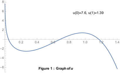
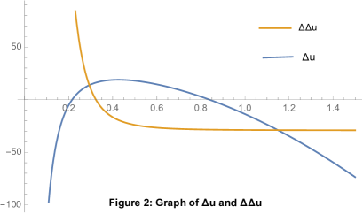
Figure 1: The graphs of $u_{k}$, $\Delta u_{k}$ and $\Delta^{2}u_{k}$ in the case $S_{1}=\{0\}$, $S_{\varphi}=\{|x|=1\}$.

 

2.2 Proof of (9), (10) and (11)

We shall now assume that we are in case $iv)$ of Theorem 1.1, i.e. $S_{1}=\{0\}$ and $S_{\varphi}=\{|x|=1\}.$

Lemma 2.2

We have

$$\Delta^{2}u_{k}(r)\leq\frac{C}{r^{4}}\quad\text{for }r\in(0,R)$$

and

$$0<-\Delta u_{k}(r)\leq\frac{C}{r^{2}}\quad\text{for }r\in(0,\theta_{2,k}),$$

where $\theta_{2,k}$ is as in Lemma 2.1.

Proof.

Using (30) and the fundamental theorem of calculus we write for $|x|\leq\theta_{4,k}$

$$\begin{split}\Delta^{2}u_{k}(x)&=\int_{|x|}^{\theta_{4,k}}\frac{1}{\omega_{5}r^{5}}\int_{B_{r}}V_{k}(y)e^{6u_{k}(y)}dydr\\ &\leq C\int_{|x|}^{\theta_{4,k}}\frac{1}{r^{5}}dr\leq\frac{C}{|x|^{4}},\end{split}$$

and for $|x|>\theta_{4,k}$ the inequality is obvious. This yields for $|x|\leq\theta_{2,k}$

$$-\Delta u_{k}(x)=\int_{|x|}^{\theta_{2,k}}\frac{1}{\omega_{5}r^{5}}\int_{B_{r}}\Delta^{2}u_{k}(y)dydr\leq\frac{C}{|x|^{2}}.$$

∎

The following estimates can be seen as an extention of Lemma 3.5 in [27], whose method of proof goes back to [29].

Lemma 2.3

Let $0<\delta<1$ be fixed. Then there exists $C=C(\delta)>0$ ($C(\delta)$ can be made independent of $\delta$ if $\delta$ lies in a compact subset of $[0,1)$) such that

• $re^{u_{k}(r)}\leq C$ for every $0\leq r\leq\delta$.

• $|(\Delta u_{k})^{\prime}(r)-\frac{r}{6}\Delta^{2}u_{k}(\delta)|\leq\frac{C}{r^{3}},\quad 0<r\leq\delta.$

• $\left|u_{k}^{\prime}(r)+\delta^{2}\frac{\Delta^{2}u_{k}(\delta)}{72}r-\frac{\Delta^{2}u_{k}(\delta)}{96}r^{3}-\frac{\Delta u_{k}(\delta)}{6}r\right|\leq\frac{C}{r},\quad 0<r\leq\delta.$

Proof.

Since $u_{k}\to-\infty$ uniformly in $(\theta_{1,k},\delta)$, we have $i)$ for $\theta_{1,k}\leq r\leq\delta$. For $0<r<\theta_{1,k}$ we use that $u_{k}$ is monotone decreasing. Indeed,

$$r^{6}e^{6u_{k}(r)}\leq C\int_{B_{r}}e^{6u_{k}(y)}dy\leq C.$$

To prove $ii)$ and $iii)$ we use Greens representation formula. We have

$$\Delta u_{k}(x) =-\int_{B_{\delta}}G(x,y)\Delta^{2}u_{k}(y)dy+\Delta u_{k}(\delta)$$

$$=-\int_{B_{\delta}}V_{k}e^{6u_{k}(z)}\left(\int_{B_{\delta}}G(x,y)G(y,z)dy\right)dz-\Delta^{2}u_{k}(\delta)\int_{B_{\delta}}G(x,y)dy+\Delta u_{k}(\delta)$$

$$=-\int_{B_{\delta}}V_{k}e^{6u_{k}(z)}\left(\int_{B_{\delta}}G(x,y)G(y,z)dy\right)dz-\Delta^{2}u_{k}(\delta)\frac{\delta^{2}-|x|^{2}}{12}+\Delta u_{k}(\delta),$$ (34)

where $G$ is the Green function for $-\Delta$ on $B_{\delta}$ with Dirichlet boundary condition. Hence, together with $i)$

$$\left|(\Delta u_{k})^{\prime}(r)-\frac{r}{6}\Delta^{2}u_{k}(\delta)\right| \leq C\int_{B_{\delta}}e^{6u_{k}(z)}\left(\int_{B_{\delta}}|\nabla_{x}G(x,y)|G(y,z)dy\right)dz,\quad r:=|x|$$

$$\leq C\int_{B_{\delta}}e^{6u_{k}(z)}\int_{B_{\delta}}\frac{dy}{|x-y|^{5}|y-z|^{4}}dz$$

$$\leq C\int_{B_{\delta}}e^{6u_{k}(z)}\frac{1}{|x-z|^{3}}dz.$$

For $x\neq 0$ we split the domain $B_{\delta}$ into

$$B_{\delta}=\cup_{i=1}^{3}A_{i},\quad A_{1}:=B_{\frac{|x|}{2}},\quad A_{2}={(B_{2|x|}\cap B_{\delta})}\setminus A_{1},\quad A_{3}:=B_{\delta}\setminus(A_{1}\cup A_{2}).$$

Using that

$$\frac{1}{|x-z|}\leq\frac{2}{|x|}\quad\text{for every }z\in A_{1}\cup A_{3},$$

and together with $i)$, we bound

$$\int_{B_{\delta}}e^{6u_{k}(z)}\frac{1}{|x-z|^{3}}dz\leq\frac{C}{|x|^{3}}\int_{A_{1}\cup A_{3}}e^{6u_{k}(z)}dz+C\int_{A_{2}}\frac{1}{|z|^{6}}\frac{1}{|x-z|^{3}}dz\leq\frac{C}{|x|^{3}}.$$

This proves $ii)$. From the identity (30) and by (2.2) one gets

$$\left|u_{k}^{\prime}(r)+\delta^{2}\frac{\Delta^{2}u_{k}(\delta)}{72}r-\frac{\Delta^{2}u_{k}(\delta)}{96}r^{3}-\frac{\Delta u_{k}(\delta)}{6}r\right|$$

$$\leq\frac{1}{\omega_{5}r^{5}}\int_{B_{r}}\int_{B_{\delta}}V_{k}e^{6u_{k}(z)}\left(\int_{B_{\delta}}G(x,y)G(y,z)dy\right)dzdx$$

$$\leq\frac{C}{r^{5}}\int_{B_{r}}\int_{B_{\delta}}e^{6u_{k}(z)}\frac{1}{|x-z|^{2}}dzdx$$

$$\leq\frac{C}{r^{5}}\int_{B_{r}}\frac{1}{|x|^{2}}dx$$

$$\leq\frac{C}{r},$$

hence also $iii)$ is proven. ∎

Proof of (9) (completed).

By assumptions $\frac{u_{k}}{\beta_{k}}\to\varphi$ in $C^{5}_{\operatorname{loc}}(B_{R}\setminus(\{0\}\cup\{|x|=1\}))$. We know that $\varphi\in C_{rad}^{\infty}(B_{R}\setminus\{0\})$ solves the ODE

$$\Delta^{3}\varphi=0\quad\text{in }(0,R),\quad\varphi(1)=0\quad\varphi^{\prime}(1)=0,\quad\varphi\not\equiv 0\quad\text{and }\varphi\leq 0.$$

Therefore, $\varphi$ is of the form

$$\varphi(r)=c_{1}+c_{2}r^{2}+c_{3}r^{4}+\frac{c_{4}}{r^{4}}+\frac{c_{5}}{r^{2}}+c_{6}\log r,$$ (35)

for some constants $c_{0},\dots,c_{6}$. This yields

$$\varphi^{\prime}(r)+\delta^{2}\frac{\Delta^{2}\varphi(\delta)}{72}r-\frac{\Delta^{2}\varphi(\delta)}{96}r^{3}-\frac{\Delta\varphi(\delta)}{6}r=-\frac{4c_{4}}{r^{5}}-\frac{2c_{5}}{r^{3}}+\frac{c_{6}}{r}+\frac{2c_{5}r}{3\delta^{4}}-\frac{8c_{5}r}{9\delta^{2}}+\frac{c_{6}r^{3}}{6\delta^{4}}.$$

Dividing by $\beta_{k}$ in $iii)$ of Lemma 2.3 and using (5) we obtain

$$-\frac{4c_{4}}{r^{5}}-\frac{2c_{5}}{r^{3}}+\frac{c_{6}}{r}+\frac{2c_{5}r}{3\delta^{4}}-\frac{8c_{5}r}{9\delta^{2}}+\frac{c_{6}r^{3}}{6\delta^{4}}\equiv 0,$$

which implies that $c_{4}=c_{5}=c_{6}=0$. Now the condition $\varphi(1)=\varphi^{\prime}(1)=0$ gives $c_{1}=c_{3}$ and $c_{2}=-2c_{3}$, that is, $\varphi(r)=c_{3}(1-r^{2})^{2}$. Since $\varphi\leq 0$ we must have $c_{3}<0$, and up to replacing $\beta_{k}$ with $|c_{3}|\beta_{k}$ we obtain $c_{3}=-1$.

It remains to prove that the convergence in (9) holds in $B_{R}\setminus\{0\}$ (and not just in $B_{R}\setminus(\{0\}\cup\{|x|=1\})$). It follows easily from the monotonicity of $\Delta^{2}u_{k}$ and from $\frac{\Delta^{2}u_{k}}{\beta_{k}}\to\Delta^{2}\varphi$ uniformly locally in $B_{R}\setminus(\{0\}\cup\{|x|=1\})$ that

$$\frac{\Delta^{2}u_{k}}{\beta_{k}}\to\Delta^{2}\varphi\quad\text{uniformly locally in }B_{R}\setminus\{0\}.$$

Then using (74) we obtain

$$\frac{\Delta u_{k}}{\beta_{k}}\to\Delta\varphi,\quad\frac{u_{k}}{\beta_{k}}\to\varphi\quad\text{uniformly locally in }B_{R}\setminus\{0\},$$

and using (1) and (30) again, we also infer the $C^{5}$-convergence claimed in (9). $\square$

In the following $\beta_{k}\to\infty$ is such that we have (9). The following is a simple consequence of Lemma 2.1 and (9).

Corollary 2.4

We have $\theta_{i,k}=o(1)$ for $i=1,\dots,4$, where $\theta_{i,k}$ is as in Lemma 2.1.

Lemma 2.5

Let $(u_{k})$ be radial solutions to (1)-(2) in $\Omega=B_{R_{0}}$, $R_{0}>0$, with $V_{k}$ as in Theorem 1.1, satisfying

$$u_{k}(x)\leq u_{k}(0)\quad\text{ on }B_{\varepsilon},$$ (36)

for some $\varepsilon\in(0,R_{0})$. Assume further that $u_{k}(0)\to\infty$, $\Delta u_{k}(0)\leq 0$ and that there are $\alpha_{k}\to\infty$, $\tau\in(0,R_{0})$ and constants $C_{1}$ and $C_{2}$ (depending on $\tau$) such that

$$\Delta u_{k}(\tau) =\alpha_{k}(C_{1}+o(1))$$ (37)

$$\Delta^{2}u_{k}(\tau) =\alpha_{k}(C_{2}+o(1)),$$ (38)

and

$$C_{3}:=C_{1}-\frac{C_{2}\tau^{2}}{12}>0.$$ (39)

Then for $r_{k}:=2e^{-u_{k}(0)}$ we have $\alpha_{k}r_{k}^{2}=o(1)$ and (11) holds.

Proof.

From (36) we infer

$$\eta_{k}\leq\eta_{k}(0)=\log 2\quad\text{for }|x|\leq\frac{\varepsilon}{r_{k}},$$ (40)

hence

$$|(-\Delta)^{3}\eta_{k}(x)|\leq C\quad\text{for }|x|\leq\frac{\varepsilon}{r_{k}}.$$ (41)

We now want to use (41) together with elliptic estimates applied to the function $\Delta\eta_{k}$ and then to $\eta_{k}$. With $\tau\in(0,1)$ fixed such that (37)-(39) hold, we obtain from (2.2)

$$\Delta\eta_{k}(x)+r_{k}^{2}\left(\frac{\Delta^{2}u_{k}(\tau)\tau^{2}}{12}-\Delta u_{k}(\tau)\right)$$

$$=r_{k}^{4}\frac{\Delta^{2}u_{k}(\tau)|x|^{2}}{12}-r_{k}^{2}\int_{B_{\tau}}e^{6u_{k}(z)}V_{k}(z)\int_{B_{\tau}}G(r_{k}x,z)G(y,z)dydz.$$

and integrating on $B_{R}$

$$\int_{B_{R}}|\Delta\eta_{k}(x)-r_{k}^{2}\alpha_{k}(C_{3}+o(1))|dx \leq Cr_{k}^{4}\alpha_{k}R^{8}+C\int_{B_{R}}\int_{B_{\tau}}e^{6u_{k}(z)}V_{k}(z)\frac{r_{k}^{2}}{|r_{k}x-z|^{2}}dzdx$$

$$\leq Cr_{k}^{4}\alpha_{k}R^{8}+CR^{4}.$$ (42)

We now claim that $\limsup_{k\to\infty}r_{k}^{2}\alpha_{k}<\infty$. Indeed, assume by contradiction that for a subsequence $r_{k}^{2}\alpha_{k}\to\infty$. Set $\tilde{\eta}_{k}:=\frac{\eta_{k}}{r_{k}^{2}\alpha_{k}}$. Then by (41), (42) and elliptic estimates $\Delta\tilde{\eta}_{k}$ is uniformly bounded in $L^{\infty}_{\operatorname{loc}}(\mathbb{R}^{6})$, and using (40) and the Harnack inequality one has $\tilde{\eta}_{k}\to\tilde{\eta}$ in $C^{5}_{\operatorname{loc}}(\mathbb{R}^{6})$ where $\tilde{\eta}$ satisfies

$$\Delta^{3}\tilde{\eta}=0\quad\text{in }\mathbb{R}^{6},\quad\int_{B_{R}}|\Delta\tilde{\eta}(x)-C_{3}|dx=0.$$

This shows that $\Delta\tilde{\eta}(0)=C_{3}>0$, which contradicts $\Delta u_{k}(0)\leq 0$. This proves our claim.

Now, up to a subsequence we set $a:=\lim_{k\to\infty}r_{k}^{2}\alpha_{k}<\infty$. With the same elliptic estimates used for $\tilde{\eta}_{k}$ we get $\eta_{k}\to\eta_{\infty}$ in $C^{5}_{\operatorname{loc}}(\mathbb{R}^{6})$ where $\eta_{\infty}$ satisfies

$$(-\Delta)^{3}\eta_{\infty}=120e^{6\eta_{\infty}}\quad\text{in }\mathbb{R}^{6},\quad\int_{\mathbb{R}^{6}}e^{6\eta_{\infty}}dx<\infty.$$

Moreover,

$$\int_{B_{R}}|\Delta\eta_{\infty}(x)-C_{3}a|dx\leq CR^{4}\quad\text{for every }R>0.$$ (43)

By Theorem D we can write $\eta_{\infty}=v+p$ with $\Delta v(x)\to 0$ as $|x|\to\infty$ and $p$ is a (radially symmetric) upper bounded polynomial of degree at most $4$. In particular $\lim_{|x|\to\infty}\Delta p(x)\leq 0$. Since $a\geq 0$, from (43) we infer that $a=0$, which is only possible if $\Delta p\equiv 0$, that is, $p$ is constant. By Theorem D, also observing that $\eta_{\infty}(0)=\log 2$, we conclude that $\eta_{\infty}=\eta$, so that (11) is proven. ∎

Proof of (10) and (11) (completed)

It follows from Lemma 2.1 and (9) that (36) holds. From (9) we get (37)-(39) with

$$\alpha_{k}=\beta_{k},\quad C_{1}=24-32\delta^{2},\quad C_{2}=-384,\quad C_{3}=24,$$

for any $\delta\in(0,1)$, so that (11) follows at once from Lemma 2.5. Moreover, the claim $\alpha_{k}r_{k}^{2}=o(1)$ of Lemma 2.5 is equivalent to (10). $\square$

2.3 Proof of (12)

Lemma 2.6

Let $p\in(1,2)$, $\delta\in(0,1)$ be fixed. Let the assumptions of Lemma 2.5 be in force and additionally assume that there exists $0<\theta_{k}=o(1)$ such that

$$0\leq-u_{k}^{\prime}(r)\leq\frac{C}{r}\quad\text{on }(0,\theta_{k})\text{ and}\quad u_{k}^{\prime}(r)\geq 0\quad\text{on }(\theta_{k},\delta).$$ (44)

Then for each $k$ large there exists $t_{k}\in(0,\theta_{k}]$ such that following hold:

• $r^{p}e^{u_{k}}$ is monotone decreasing on $(c_{p}r_{k},t_{k})$ for some constant $c_{p}>0$.

• $r_{k}=o(t_{k})$ as $k\to\infty$,

• $u_{k}(t_{k})\leq u_{k}(\theta_{k})+C.$

Finally, if $u_{k}(\delta)\to-\infty$, we conclude

$$\lim_{k\to\infty}\int_{B_{\delta}}V_{k}e^{6u_{k}}dx=\Lambda_{1}.$$ (45)

Proof.

For the proof of $i)$ and $ii)$ we shall follow [27]. We set $c_{p}=\sqrt{1+\frac{p}{2-p}}$. For any $L>c_{p}$ and for $r\in(c_{p}r_{k},Lr_{k})$, using (11), which follows from Lemma 2.5, we get

$$(r^{p}e^{u_{k}(r)})^{\prime}(r) =\left(pr^{p-1}+r^{p}u_{k}^{\prime}(r)\right)e^{u_{k}(r)}$$

$$=r^{p-1}\left(p+\rho r_{k}u_{k}^{\prime}(\rho r_{k})\right)e^{u_{k}(r)},\quad\rho:=\frac{r}{r_{k}}\in(c_{p},L)$$

$$=r^{p-1}\left(p+\rho\left(\frac{-2\rho}{1+\rho^{2}}+o(1)\right)\right)e^{u_{k}(r)}$$

$$<r^{p-1}\left(\frac{p-2}{1+\rho^{2}}+o(1)\right)e^{u_{k}(r)}$$

$$<0,$$

where $o(1)\to 0$ as $k\to\infty$ uniformly on $\rho\in(c_{p},L)$. We set

$$t_{k}:=\inf\{r\in(c_{p}r_{k},\theta_{k}):(r^{p}e^{u_{k}(r)})^{\prime}(r)=0\}.$$

It is easy to see that $t_{k}$ is well defined, $r_{k}=o(t_{k})$ and $r^{p}e^{u_{k}(r)}$ is monotone decreasing on $(c_{p}r_{k},t_{k})$.

Now we prove $iii)$ in few steps.

Step 1 $t_{k}e^{u_{k}(t_{k})}\to 0$.

It follows from $i)$ that $re^{u_{k}}$ is monotone decreasing on $(c_{p}r_{k},t_{k})$. Using that $r_{k}=o(t_{k})$ and (11) we obtain for any $L>c_{p}$ and for $k$ large

$$t_{k}e^{u_{k}(t_{k})}\leq Lr_{k}e^{u_{k}(Lr_{k})}=L\left(\frac{2}{1+L^{2}}+o(1)\right),\quad o(1)\xrightarrow{k\to\infty}0.$$ (46)

Taking $k\to\infty$ and then taking $L\to\infty$ one has Step 1.

Step 2 There exists $C>0$ such that $\theta_{k}\leq Ct_{k}.$

We assume by contradiction that $\frac{\theta_{k}}{t_{k}}\to\infty$. Then for any $\varepsilon>0$ we have $u_{k}^{\prime}(rt_{k})<0$ for $r\in(\varepsilon,\tfrac{1}{\varepsilon})$ and $k\geq k_{0}(\varepsilon)$ large, thanks to (44). Then, setting

$$\bar{u}_{k}(r)=u_{k}(rt_{k})-u_{k}(t_{k}).$$

we get for $k\geq k_{0}(\varepsilon)$

$$0<-\bar{u}_{k}^{\prime}(r)\leq\frac{C}{r},\quad r\in(\varepsilon,\tfrac{1}{\varepsilon}).$$ (47)

Hence, $\bar{u}_{k}\to\bar{u}_{\infty}$ in $C^{0}_{\operatorname{loc}}(0,\infty)$. By (46) we have

$$(-\Delta)^{3}\bar{u}_{k}(r)=V_{k}(t_{k}r)t_{k}^{6}e^{6u_{k}(t_{k})}e^{6\bar{u}_{k}}=o(1)e^{6\bar{u}_{k}}$$

with $o(1)\to 0$ locally uniformly for $r\in[0,\infty)$, thanks to Step 1. Then, by elliptic estimates $\bar{u}_{k}\to\bar{u}_{\infty}$ also in $C^{5}_{\operatorname{loc}}(0,\infty)$ where $\Delta^{3}u_{\infty}\equiv 0$ in $\mathbb{R}^{6}\setminus\{0\}$

$$|\bar{u}_{\infty}(r)|\leq\frac{C}{r},\text{ for }r\in(0,\infty),\quad\bar{u}_{\infty}(1)=0,\quad\bar{u}_{\infty}^{\prime}(1)=-p.$$

Since $\bar{u}_{\infty}$ is radial, it is of the form given in (35), and hence $\bar{u}_{\infty}(r)=-p\log r$. Using that $r_{k}=o(t_{k})$ and (11) one has

$$64p+o(1)=-t_{k}^{5}(\Delta^{2}u_{k})^{\prime}(t_{k})=\frac{1}{\omega_{5}}\int_{B_{t_{k}}}V_{k}e^{6u_{k}}dx\geq\frac{\Lambda_{1}}{\omega_{5}}+o(1)=128+o(1),$$

a contradiction as $p<2$.

Step 3 $u_{k}(t_{k})\leq u_{k}(\theta_{k})+C$.

Since taking $\varepsilon$ sufficiently small (47) holds for every $r\in(\varepsilon,\tfrac{\theta_{k}}{t_{k}})$, we have

$$u_{k}(t_{k}) =u_{k}(\theta_{k})-\int_{1}^{\frac{\theta_{1,k}}{t_{k}}}\bar{u}_{k}^{\prime}(r)dr$$

$$\leq u_{k}(\theta_{k})+C\log\frac{\theta_{k}}{t_{k}}$$

$$\leq u_{k}(\theta_{k})+C,$$

thanks to Step 2.

Step 4 (45) holds for $\delta$ such that $u_{k}(\delta)\to-\infty$.

Since $u_{k}(\theta_{k})<u_{k}(\delta)$ for $k$ large, we conclude

$$u_{k}(t_{k})\leq u_{k}(\theta_{k})+C\leq u_{k}(\delta)+C\to-\infty\quad\text{as }k\to\infty.$$

Splitting the domain $B_{\delta}$ into

$$B_{\delta}=\cup_{i=1}^{3}A_{i},\quad A_{1}:=B_{Lr_{k}},\quad A_{2}:=B_{t_{k}}\setminus B_{Lr_{k}},\quad A_{3}:=B_{\delta}\setminus B_{t_{k}},$$

we write

$$\int_{B_{\delta}}V_{k}e^{6u_{k}}dx=\sum_{i=1}^{3}I_{i},\quad I_{i}:=\int_{A_{i}}V_{k}e^{6u_{k}}dx.$$

Using the monotonicity of $u_{k}$ we infer

$$\max_{[t_{k},\delta]}u_{k}=\max\{u_{k}(t_{k}),u_{k}(\delta)\}\xrightarrow{k\to\infty}-\infty,$$

which gives $I_{3}\to 0$ as $k\to\infty$. For $L$ large we have $r^{p}e^{u_{k}(r)}$ monotone decreasing on $(Lr_{k},t_{k})$, and hence

$$I_{2}\leq C\int_{A_{2}}|x|^{6p}e^{6u_{k}(x)}\frac{1}{|x|^{6p}}dx\leq C(Lr_{k})^{6}e^{6u_{k}(Lr_{k})}\xrightarrow{k\to\infty}C\left(\frac{L}{1+L^{2}}\right)^{6},$$

so that

$$\lim_{L\to\infty}\lim_{k\to\infty}I_{2}=0.$$

Finally

$$\lim_{L\to\infty}\lim_{k\to\infty}I_{1}=\Lambda_{1}$$

by (11). The proof of (45) follows immediately. ∎

Proof of (12) (completed).

In the proof of (11) we have already verified that the assumptions of Lemma 2.5 are in force. We claim that also (44) holds with $\theta_{k}=\theta_{1,k}$, where $\theta_{1,k}$ is given by Lemma 2.1.

Indeed for $k$ sufficiently large, since $\Delta\varphi(\tfrac{1}{2})>0$, (9) implies that $\Delta u_{k}(\tfrac{1}{2})>0$, hence by (27) we have $\Delta u_{k}>0$ on $(\theta_{2,k},\frac{1}{2}]$. Together with Lemma 2.2 this gives

$$-\Delta u_{k}(r)\leq\frac{C}{r^{2}}\quad\text{on }(0,\tfrac{1}{2}],$$

hence $-u_{k}^{\prime}\leq\frac{C}{r}$ on $(0,\tfrac{1}{2}]$. Then (44) follows.

Now observe that (9) implies $u_{k}(\delta)\to-\infty$ for $\delta\in(0,1)$. Then (12) follow from Lemma 2.6 $\square$

3 Proof of Theorem 1.2

Let $V_{k}$, $V_{\infty}$ and $P(r):=-ar^{2}-br^{4}$ be as in the statement of Theorem 1.2. If we can find $\tilde{u}_{k}$ satisfying the requests of the theorem with $V_{k}$ replaced by $\tilde{V}_{k}:=V_{k}e^{P}$, then $u_{k}:=\tilde{u}_{k}+\frac{P}{6}$ will satisfy the requests of the theorem with the original $V_{k}$. Therefore there is no loss of generality in assuming that $P\equiv 0$, i.e. $V_{\infty}^{\prime}\leq 0$.

Taking $\lambda=\lambda_{k}\in(0,\frac{1}{24}]$ in Theorem E we have that for every $\Lambda>0$ there exists a solution $u_{k}\in C^{5}_{rad}(\mathbb{R}^{6})$ to

$$u_{k}(x) =v_{k}-|x|^{4}+c_{k}$$

$$=\frac{1}{\gamma_{6}}\int_{\mathbb{R}^{6}}\log\left(\frac{1}{|x-y|}\right)V_{k}(y)e^{-6|y|^{4}}e^{6(v_{k}(y)+c_{k})}dy$$

$$\quad+\lambda_{k}\Delta v_{k}(0)(|x|^{4}-2|x|^{2})-|x|^{4}+c_{k}$$

such that

$$\Lambda=\int_{\mathbb{R}^{6}}V_{k}(y)e^{6u_{k}(y)}dy.$$ (48)

In particular $u_{k}$ solves the integral equation

$$u_{k}(x)=\frac{1}{\gamma_{6}}\int_{\mathbb{R}^{6}}\log\left(\frac{1}{|x-y|}\right)V_{k}(y)e^{6u_{k}(y)}dy+\lambda_{k}\Delta u_{k}(0)(1-|x|^{2})^{2}-|x|^{4}+\tilde{c}_{k},$$ (49)

where

$$\tilde{c_{k}}:=c_{k}-\lambda_{k}\Delta u_{k}(0).$$

Computing the Laplacian at the origin on both sides of (49) yields

$$(1+24\lambda_{k})\Delta u_{k}(0)=-\frac{4}{\gamma_{6}}\int_{\mathbb{R}^{6}}\frac{V_{k}(y)e^{6u_{k}(y)}}{|y|^{2}}dy,$$ (50)

hence

$$\Delta u_{k}(0)<0.$$ (51)

We will now prove Theorem 1.2 by fixing $\Lambda>\Lambda_{1}$, letting $\lambda_{k}\to 0^{+}$. The case $\Lambda=\Lambda_{1}$ can be easily deduced by first taking $\Lambda>\Lambda_{1}$ and then letting $\Lambda\to\Lambda_{1}^{+}$ slowly enough with a diagonal procedure.

The first step will be proving that $\lambda_{k}\Delta u_{k}(0)\to-\infty$ (so that $-\lambda_{k}\Delta u_{k}(0)$ plays the role of $\beta_{k}$ from Theorem A and Theorem 1.1). A crucial tool will be the following Pohozaev-type identity, from [31, Lemma 2.4] (see also [32, Theorem 2.1]) for $w$ solving

$$w(x)=\frac{1}{\gamma_{6}}\int_{\mathbb{R}^{6}}\log\left(\frac{|y|}{|x-y|}\right)K(y)e^{6w(y)}dy+c$$

with $|x\cdot\nabla K(x)|\leq C$, and

$$\alpha:=\int_{\mathbb{R}^{6}}Ke^{nw}dy,$$

we have

$$\frac{\alpha}{\gamma_{6}}\left(\frac{\alpha}{\gamma_{6}}-2\right)=\frac{1}{3\gamma_{6}}\int_{\mathbb{R}^{6}}\left(y\cdot\nabla K(y)\right)e^{6w(y)}dy,$$

which, observing that $2\gamma_{6}=\Lambda_{1}$, can be recast as

$$\frac{2\alpha}{\Lambda_{1}}\left(\alpha-\Lambda_{1}\right)=\frac{1}{3}\int_{\mathbb{R}^{6}}\left(y\cdot\nabla K(y)\right)e^{6w(y)}dy.$$ (52)

Lemma 3.1

Let $\Lambda>\Lambda_{1}$. Let $(u_{k})$ be a sequence of radial solutions to (49)-(48) with $V_{k}$ as in Theorem 1.2. Then $\lambda_{k}\Delta u_{k}(0)\to-\infty$.

Proof.

We proceed by steps.

Step 1 $u_{k}(x)\leq 16+u_{k}(2)-|x|^{4}$ for $|x|\geq 2$.

Differentiating under the integral sign and observing that $\Delta\log\frac{1}{|\cdot-y|}\leq 0$, from (49), we obtain

$$\Delta\tilde{u}_{k}\leq 0,\quad\tilde{u}_{k}(x):=u_{k}(x)-\lambda_{k}\Delta u_{k}(0)(1-|x|^{2})^{2}+|x|^{4},$$

and by (30) we have that $\tilde{u}_{k}$ is monotone decreasing. This proves Step 1, thanks to (51).

Step 2 For every $\delta>0$ we have $\sup_{B_{\delta}}u_{k}\to\infty$.

Assume by contradiction that $\sup_{k}\sup_{B_{\delta}}u_{k}<\infty$ for some $\delta>0$. Then by (48)-(50) one has $|\Delta u_{k}(0)|\leq C$, which implies that $\lambda_{k}\Delta u_{k}(0)\to 0$. Then, by Theorem A, up to a subsequence either $(u_{k})$ is bounded in $C^{5,\sigma}_{\operatorname{loc}}(\mathbb{R}^{6})$ for $\sigma\in[0,1)$, or there exists $\beta_{k}\to\infty$ such that

$$\frac{u_{k}}{\beta_{k}}\to\varphi:=c_{1}+c_{2}r^{2}+c_{3}r^{4}\quad\text{in }C^{5}_{\operatorname{loc}}(\mathbb{R}^{6}),\quad\varphi\leq 0,\quad\varphi\not\equiv 0,$$

for some $c_{1},c_{2},c_{3}\in\mathbb{R}$. We claim that the latter case does not occur. Otherwise, differentiating under the integral sign in (49), one gets $\int_{B_{r}}|\Delta u_{k}|dx\leq C(r)$, hence $\Delta\varphi\equiv 0$ in $\mathbb{R}^{6}$, that is, $\varphi\equiv c_{1}<0$. Then $u_{k}\to-\infty$ locally uniformly in $\mathbb{R}^{6}$, and by Step 1, $\int_{\mathbb{R}^{6}}V_{k}e^{6u_{k}}dx\to 0$, a contradiction to (48). Thus, up to a subsequence, $u_{k}\to u_{\infty}$ in $C^{5}_{\operatorname{loc}}(\mathbb{R}^{6})$. We claim that $u_{\infty}$ satisfies

$$u_{\infty}(x)=\frac{1}{\gamma_{6}}\int_{\mathbb{R}^{6}}\log\left(\frac{1}{|x-y|}\right)V_{\infty}(y)e^{6u_{\infty}(y)}dy-|x|^{4}+c=:\bar{u}_{\infty}(x),$$

with

$$\alpha:=\int_{\mathbb{R}^{6}}V_{\infty}e^{6u_{\infty}}dx=\Lambda,\quad c:=\lim_{k\to\infty}\tilde{c}_{k}.$$

It follows from Step 1 that $u_{\infty}(x)\leq C-|x|^{4}$ on $\mathbb{R}^{6}$. Using this one can show that $u_{k}\to\bar{u}_{\infty}$ in $C^{0}_{loc}(\mathbb{R}^{6})$, and hence $u_{\infty}=\bar{u}_{\infty}$.

To show that $\alpha=\Lambda$ we use Step 1. Indeed, as $u_{k}(2)\leq C$

$$\alpha=\lim_{L\to\infty}\lim_{k\to\infty}\int_{B_{L}}V_{k}e^{6u_{k}}dx=\Lambda-\lim_{L\to\infty}\lim_{k\to\infty}\int_{B_{L}^{c}}V_{k}e^{6u_{k}}dx=\Lambda.$$

Since $V_{\infty}^{\prime}\leq 0$, applying (52) with $w=u_{\infty}+|x|^{4}$ and $K=V_{\infty}e^{-|x|^{4}}$ one gets $\alpha<\Lambda_{1}$, a contradiction as $\alpha>\Lambda_{1}$.

Step 3 $\lambda_{k}\Delta u_{k}(0)\to-\infty$

We assume by contradiction that $\lambda_{k}\Delta u_{k}(0)\geq-C$ for some $C>0$. Then, differentiating in (49) and using Fubini’s theorem, we get for every $R_{0}>0$

$$\int_{B_{2R_{0}}}|\nabla u_{k}(x)|dx\leq C(R_{0}).$$

Therefore, by [21, Theorem 1] (see also [28]), as $u_{k}$ is radially symmetric

$$\int_{B_{R_{0}}}V_{k}e^{6u_{k}}dx\to\Lambda_{1}.$$

Set now $\varepsilon_{0}=\frac{1}{2}(\Lambda-\Lambda_{1})$ and fix $R_{0}=R_{0}(\varepsilon,\Lambda)$ such that

$$\int_{B_{R_{0}}^{c}}V_{k}e^{6u_{k}}dx\leq C\int_{B_{R_{0}}^{c}}e^{-|x|^{4}}dx<\varepsilon_{0}.$$

Then we obtain

$$\Lambda=\int_{B_{R_{0}}}V_{k}e^{6u_{k}}dx+\int_{B_{R_{0}}^{c}}V_{k}e^{6u_{k}}dx<\frac{\Lambda+\Lambda_{1}}{2}+o(1),$$

which is a contradiction. ∎

Lemma 3.2

Under the same assumptions of Lemma 3.1, we have that $u_{k}(0)\to\infty$ and (11)-(12) hold with $r_{k}=2e^{-u_{k}(0)}$ and any $\delta\in(0,1)$.

Proof.

We proceed by steps.

Step 1 There exists a radius $\xi_{k}\to 1$ such that $\xi_{k}$ is a local maxima of $u_{k}$. Indeed differentiating (49) under the integral sign we obtain

$$u_{k}^{\prime}(r) =\frac{1}{\omega_{5}r^{5}}\int_{B_{r}}\Delta u_{k}(x)dx$$

$$=C\frac{1}{r^{5}}\int_{\mathbb{R}^{6}}V_{k}(y)e^{6u_{k}(y)}\int_{B_{r}}\frac{dx}{|x-y|^{2}}dy-\frac{1}{\omega_{5}r^{5}}\int_{B_{r}}\Delta\left(-\lambda_{k}\Delta u_{k}(0)(1-|x|^{2})^{2}+|x|^{4}\right)dx$$

$$=\frac{O(1)}{r}-4\lambda_{k}\Delta u_{k}(0)r(1-r^{2})-4r^{3}.$$ (53)

Then, using Lemma 3.1 we infer

$$u_{k}^{\prime}\xrightarrow{k\to\infty}+\infty\quad\text{uniformly locally in }(0,1)$$

and

$$u_{k}^{\prime}\xrightarrow{k\to\infty}-\infty\quad\text{uniformly locally in }(1,\infty).$$

This proves the claim.

Step 2 We claim that $u_{k}(0)\to\infty$. Indeed a simple application of (30), together with $\Delta^{3}u_{k}<0$ implies that $u_{k}$ can have at most two local maxima (compare to the proof of Lemma 2.1). From (51) and the previous step we infer that $0$ and $\xi_{k}$ are these local maxima. Since $\xi_{k}\to 1$, the claim now follows at once from Step 2 of Lemma 3.1.

Step 3 We claim that $u_{k}$ satisfies (11). Indeed, as $u_{k}(0)\to\infty$, $u_{k}(0)$ is the global maximum of $u_{k}$ on $[0,\frac{1}{2}]$ and $u_{k}\to-\infty$ locally uniformly in $(0,\frac{1}{2}]$. Then we can apply Lemma 2.5 with $\alpha_{k}=-\lambda_{k}\Delta u_{k}(0)\to+\infty$ (by Lemma 3.1), $C_{1}=24-32\tau^{2}$, $C_{2}=-384$ and $C_{3}=24$ for some $\tau\in(0,\tfrac{1}{2}]$ to obtain that (11).

Step 4 (12) hold for every $\delta\in(0,1)$.

Let us verify that the assumptions of Lemma 2.6 are satisfied for any fixed $\delta\in(0,1)$. From Step 1 and Step 2 we can find $\theta_{k}\in(0,1)$ such that (44) holds, while the assumptions of Lemma 2.5 have already been verified. Moreover $u_{k}(\theta_{k})\leq u_{k}(\delta)\to-\infty$. Then (12) follows from Lemma 2.6. ∎

Proof of Theorem 1.2 (completed). Taking into account Lemma 3.2, if we show that $u_{k}(1)\to\infty$, then we are in case $iv)$ of Theorem 1.1 with $\rho=1$.

From (49) we bound

$$u_{k}(1) \geq\frac{1}{\gamma_{6}}\int_{|e_{1}-y|>1}\log\left(\frac{1}{|e_{1}-y|}\right)V_{k}(y)e^{6u_{k}(y)}dy-1+\tilde{c}_{k},$$

where $e_{1}=(1,0,\dots,0)$ is a unit vector. By Step 1 of Lemma 3.1

$$\int_{|e_{1}-y|>1}\log\left(\frac{1}{|e_{1}-y|}\right)V_{k}(y)e^{6u_{k}(y)}dy=O(1).$$

We claim that $\tilde{c}_{k}\to\infty$. In order to prove the claim we set

$$\mathcal{C}_{r}:=\{x=(x_{1},\bar{x})\in\mathbb{R}^{6}:|\bar{x}|\leq rx_{1}\}.$$

Since $u_{k}$ is radial and satisfies (48), we can choose $r_{0}>0$ small such that

$$\int_{\mathcal{C}_{2r_{0}}}V_{k}e^{6u_{k}}dx\leq\frac{\Lambda_{1}}{4}.$$

Hence, for $x\in\mathcal{C}_{r_{0}}\setminus B_{\frac{1}{2}}$

$$u_{k}(x)\leq C+\frac{1}{\gamma_{6}}\int_{\mathcal{C}_{2r_{0}}}\log\left(\frac{1}{|x-y|}\right)V_{k}(y)e^{6u_{k}(y)}dy+\lambda_{k}\Delta u_{k}(0)(1-|x|^{2})^{2}+\tilde{c}_{k}.$$

Then by Jensen’s inequality and Fubini’s theorem

$$\int_{\mathcal{C}_{r_{0}}\setminus B_{\frac{1}{2}}}V_{k}(x)e^{6u_{k}(x)}dx \leq Ce^{6\tilde{c}_{k}}\int_{\mathcal{C}_{2r_{0}}}\frac{f_{k}(y)}{\|f_{k}\|}\int_{C_{r_{0}}}V_{k}(x)\frac{e^{6\lambda_{k}\Delta u_{k}(0)(1-|x|^{2})^{2}}}{|x-y|^{p}}dxdy$$

$$=e^{6\tilde{c}_{k}}o(1),$$

thanks to Lemma 3.1, where $f_{k}:=V_{k}e^{6u_{k}}$, $\|f_{k}\|:=\|f_{k}\|_{L^{1}(\mathcal{C}_{2r_{0}})}$ and $p:=\frac{6}{\gamma_{6}}\|f_{k}\|<6$. Observing that by Lemma 3.2

$$0 <\Lambda-\Lambda_{1}=\int_{\mathbb{R}^{6}\setminus B_{\frac{1}{2}}}V_{k}e^{6u_{k}}+o(1)\leq C(r_{0})\int_{C_{r_{0}}\setminus B_{\frac{1}{2}}}V_{k}e^{6u_{k}}dx+o(1),$$

we conclude our claim.

This proves that $u_{k}(1)\to\infty$, hence we are in case $iv)$ of Theorem 1.1. Then from (9) and Step 1 of Lemma 3.1 it follows

$$\int_{B_{1+\varepsilon}\setminus B_{1-\varepsilon}}V_{k}e^{6u_{k}}dx=\Lambda-\Lambda_{1}+o(1)$$

for every $\varepsilon\in(0,1)$. $\square$

4 The case of dimension $2n\geq 6$

Similar to Theorem 1.2 one can prove the following.

Theorem 4.1

Let $(V_{k})\subset C^{0}_{rad}(\mathbb{R}^{2n})$ be positive functions with $V_{k}\to V_{\infty}$ uniformly, where $V_{\infty}\in C^{1}(\mathbb{R}^{2n})$, $V_{\infty}(0)=(2n-1)!$ and for some $a,b\geq 0$

$$\frac{d}{dr}\left(\frac{V_{\infty}(r)}{e^{ar^{2}+br^{4}}}\right)\leq 0,\quad r\in[0,\infty).$$ (54)

Then for every $\Lambda\geq\Lambda_{1}$ there exists a sequence $(u_{k})\subset C^{2n}_{rad}(\mathbb{R}^{2n})$ of solutions to (1)-(2) with $\Omega=\mathbb{R}^{2n}$ such that $u_{k}(0)\to\infty$ and $u_{k}(1)\to\infty$ as $k\to\infty$, and for every $\varepsilon\in(0,1)$

$$\lim_{k\to\infty}\int_{B_{1+\varepsilon}\setminus B_{1-\varepsilon}}V_{k}e^{2nu_{k}}dx=\Lambda-\Lambda_{1},$$ (55)

$$\lim_{k\to\infty}\int_{\mathbb{R}^{2n}\setminus(B_{\varepsilon}\cup(B_{1+\varepsilon}\setminus B_{1-\varepsilon})}V_{k}e^{2nu_{k}}dx=0.$$ (56)

Proof.

Again using the existence result of [11], for $n\geq 3$, $\lambda_{k}\in(0,\frac{1}{8n})$ and $\Lambda>\Lambda_{1}=(2n-1)!|S^{2n}|$ we find a solution to

$$u_{k}(x)=\frac{1}{\gamma_{2n}}\int_{\mathbb{R}^{2m}}\log\left(\frac{1}{|x-y|}\right)V_{k}(y)e^{2mu_{k}(y)}dy+\lambda_{k}\Delta u_{k}(0)(1-|x|^{2})^{2}-|x|^{4}+\tilde{c}_{k},$$ (57)

such that $\Delta u_{k}(0)<0$ and

$$\int_{\mathbb{R}^{2n}}V_{k}e^{2nu_{k}}dx=\Lambda.$$

Differentiating under the integral sign, and using that

$$\Delta^{3}\log\frac{1}{|x|}=-\frac{8(m-2)[(m-5)^{2}-1]}{|x|^{6}}\quad\text{in }\mathbb{R}^{m},$$

we see that

$$\Delta^{3}u_{k}<0\quad\text{in }\mathbb{R}^{2n}.$$

We now send $\lambda_{k}\to 0^{+}$ and want to show that $u_{k}(0)\to\infty$ and $u_{k}(1)\to\infty$. This can be done in the following steps.

Step 1 $\lambda_{k}\Delta u_{k}(0)\to-\infty$. In particular, $\sup_{B_{\delta}(0)}u_{k}\to\infty$ for every $\delta>0$. This can be proven with the same argument of Lemma 3.1.

Step 2 There exists $\beta_{k}\to\infty$ such that

$$\frac{u_{k}}{\beta_{k}}\to\varphi\quad\text{in }C^{2n-1}_{loc}({\mathbb{R}^{2n}}\setminus S),\quad\varphi=-c_{1}(1-|x|^{2})^{2}+c_{2},$$

for some $c_{1}\geq 0,\,c_{2}\leq 0$, where $S=\{0\}\cup S_{\varphi}$.

From (57) we see that $\varphi$ should be of the form $\varphi=-c_{1}(1-|x|^{2})^{2}+c_{2}$ for some $c_{1},c_{2}\in\mathbb{R}$. Since $\varphi\leq 0$ on $\mathbb{R}^{2n}$, we get $c_{1}\geq 0$ and $c_{2}\leq 0$.

Step 3 (Monotonicity) $u_{k}$ has two local maximum points, namely $0$ and a point $\xi_{k}\to 1$. Indeed, since $\Delta u_{k}(0)<0$, $0$ is a local maxima and the existence of $\xi_{k}$ follows as in Step 1 of Lemma 3.2. To show that $u_{k}$ can not have another point of local maxima we need to use that $\Delta^{3}u_{k}<0$ in $\mathbb{R}^{2n}$. First we show that the same conclusion of Lemma 2.1 holds. We can repeat the same proof simply replacing (32) by

$$u_{k}(1\pm\delta)\to-\infty,\quad u_{k}^{\prime}(1-\delta)\to\infty,\quad u_{k}^{\prime}(1+\delta)\to-\infty,$$

which follows from (57).

Step 4 $u_{k}(0)\to\infty$ and $u_{k}(0)=\sup_{B_{\frac{1}{2}}}u_{k}$. This follows trivially from the above steps.

Step 5 Blow-up at the origin is spherical. This can be proven as in Lemma 2.5.

Step 6 There is concentration at the origin. This can be done as in subsection 2.3.

Step 7 $u_{k}(1)\to\infty$. It suffices to show that the constant (appearing in (57)) $\tilde{c}_{k}\to\infty$. The proof is exactly as the case of dimension $6$. ∎

5 Proof of Theorem 1.3

5.1 Proof of (17) and (18)

We will now establish some relations among $\theta_{i,k}$, $\beta_{k}$ and $u_{k}(0)$ that will lead to the proofs of (17) and (18). We start with a preliminary lemma.

Lemma 5.1

For every $0<\xi_{k}<\tilde{\xi}_{k}$ with $r_{k}=o(\xi_{k})$ and $\tilde{\xi}_{k}=o(\theta_{4,k})$ we have

$$\Delta^{2}u_{k}(x)=\frac{32+o(1)}{|x|^{4}}\quad\text{on }B_{\tilde{\xi}_{k}}\setminus B_{\xi_{k}}.$$

In particular,

$$\int_{B_{t}}\Delta^{2}u_{k}(x)dx=16\omega_{5}(1+o(1))t^{2}\quad\text{for }\xi_{k}\leq t\leq\tilde{\xi}_{k}.$$

Proof.

Using (11), (12) and recalling that $\frac{\Lambda_{1}}{\omega_{5}}=128$ we obtain for $\xi_{k}\leq|x|\leq\tilde{\xi}_{k}$

$$\Delta^{2}u_{k}(x) =\int_{|x|}^{\theta_{4,k}}\frac{1}{\omega_{5}t^{5}}\int_{B_{t}}V_{k}(y)e^{6u_{k}(y)}dydt$$

$$=(\Lambda_{1}+o(1))\int_{|x|}^{\theta_{4,k}}\frac{1}{\omega_{5}t^{5}}dt$$

$$=(32+o(1))\frac{1}{|x|^{4}}.$$

The second part follows from the first part and Lemma 2.2. ∎

From the definition of $\theta_{i,k}$ one has $\Delta^{\frac{i}{2}}u_{k}(\theta_{i,k})=0$ for $i=2,4$ and $(\Delta^{\frac{i-1}{2}}u_{k})^{\prime}(\theta_{i,k})=0$ for $i=1,3$.

Lemma 5.2

We have

• $\theta_{i,k}e^{u_{k}(0)}\to\infty$ for $i=0,1,2,3,4$.

• $\beta_{k}\theta_{4,k}^{4}\to\frac{1}{12}$.

• $\beta_{k}\theta_{2,k}^{2}\to\frac{1}{3}.$

• $\theta_{3,k}\approx\theta_{4,k}$

• $\theta_{1,k}\approx\theta_{2,k}$

Proof.

$i)$ follows from the definition of $\theta_{i,k}$ and (11).

Since $\Delta^{2}(1-r^{2})^{2}=384$, by (9) and (12) we have

$$0 =\Delta^{2}u_{k}(\theta_{4,k})=\Delta^{2}u_{k}\left(\tfrac{1}{2}\right)+\int_{\theta_{4,k}}^{\frac{1}{2}}\frac{1}{\omega_{5}r^{5}}\int_{B_{r}}V_{k}e^{6u_{k}}dxdr$$

$$=(-384+o(1))\beta_{k}+(\Lambda_{1}+o(1))\int_{\theta_{4,k}}^{\frac{1}{2}}\frac{1}{\omega_{5}r^{5}}dr$$

$$=(-384+o(1))\beta_{k}+(\Lambda_{1}+o(1))\frac{1}{4\omega_{5}\theta_{4,k}^{4}}+C,$$

hence

$$\lim_{k\to\infty}\beta_{k}\theta_{4,k}^{4}=\frac{\Lambda_{1}}{1536\omega_{5}}=\frac{1}{12},$$

and this proves $ii)$.

To prove $iii)$ fix $\varepsilon>0$ arbitrarily small. Then by Lemma 2.2 and (9) we get

$$(24-32\varepsilon^{2}+o(1))\beta_{k} =\Delta u_{k}(\varepsilon)-\Delta u_{k}(\theta_{2,k})$$

$$=\int_{\theta_{2,k}}^{\varepsilon}\frac{1}{\omega_{5}t^{5}}\int_{B_{t}}\Delta^{2}u_{k}(x)dxdt$$ (58)

$$\leq\frac{C}{\theta_{2,k}^{2}}.$$

This shows that $\beta_{k}\theta_{2,k}^{2}\leq C$, and in particular $\theta_{2,k}=o(\theta_{4,k})$, thanks to $ii)$. Therefore, we can choose $\xi_{k}\in(\theta_{2,k},\theta_{4,k})$ such that $\theta_{2,k}=o(\xi_{k})$ and $\xi_{k}=o(\theta_{4,k})$.

We write the integral in (58) as $I_{1}+I_{2}$ where

$$I_{1}:=\int_{\theta_{2,k}}^{\xi_{k}}\frac{1}{\omega_{5}t^{5}}\int_{B_{t}}\Delta^{2}u_{k}(x)dxdt,\quad I_{2}:=\int_{\xi_{k}}^{\varepsilon}\frac{1}{\omega_{5}t^{5}}\int_{B_{t}}\Delta^{2}u_{k}(x)dxdt.$$

Using Lemma 5.1 we compute

$$I_{1}=16(1+o(1))\int_{\theta_{2,k}}^{\xi_{k}}\frac{1}{t^{3}}dt=\frac{8+o(1)}{\theta_{2,k}^{2}}.$$

Using that $-C\beta_{k}\leq\Delta^{2}u_{k}(x)\leq\frac{C}{|x|^{4}}$ we bound

$$|I_{2}|\leq C\varepsilon^{2}\beta_{k}+\frac{C}{\xi_{k}^{2}}=C\varepsilon^{2}\beta_{k}+\frac{o(1)}{\theta_{2,k}^{2}}.$$

Now $iii)$ follows from (58) as $\varepsilon>0$ is arbitrary and $\theta_{2,k}^{2}\beta_{k}\leq C$.

We now prove $iv)$. From Lemma 2.1 we have $\theta_{4,k}<\theta_{3,k}$. Taking $r=\theta_{3,k}$ in $ii)$ of Lemma 2.3 we have $\theta_{3,k}^{4}\beta_{k}\leq C$, and hence $\theta_{3,k}=O(\theta_{4,k})$, thanks to $ii)$.

Finally, we prove $v)$. From Lemma 2.1 we have $\theta_{2,k}<\theta_{1,k}$. Taking $r=\theta_{1,k}$ in $iii)$ of Lemma 2.3 we have $\theta_{1,k}^{2}\beta_{k}\leq C$, and hence $\theta_{1,k}=O(\theta_{2,k})$, thanks to $iii)$. ∎

Lemma 5.3

We have

$$\lim_{k\to\infty}\frac{\Delta u_{k}(\theta_{3,k})}{\beta_{k}}=\Delta\varphi(0)=24.$$

Proof.

Since $\Delta\varphi(\frac{\sqrt{3}}{2})=0$, there exists a sequence $\tilde{\theta}_{2,k}\to\frac{\sqrt{3}}{2}$ such that $\Delta u_{k}(\tilde{\theta}_{2,k})=0$. Hence, by Lemma 2.1 we infer

$$0\leq-\Delta^{2}u_{k}(r)\leq-\Delta^{2}u_{k}(\tilde{\theta}_{2,k}),\quad\text{for }\theta_{3,k}\leq r\leq\tilde{\theta}_{2,k},$$

and with (9) we get

$$\Delta u_{k}(\theta_{3,k}) =\int_{\theta_{3,k}}^{\tilde{\theta}_{2,k}}\frac{1}{\omega_{5}t^{5}}\int_{B_{t}}(-\Delta^{2}u_{k}(x))dxdt\leq-\Delta^{2}u_{k}(\tilde{\theta}_{2,k})\frac{\tilde{\theta}_{2,k}^{2}-\theta_{3,k}^{2}}{12}=(24+o(1))\beta_{k}.$$

The lemma follows immediately by (9). ∎

Proof of (17) and (18) (completed).

According to Lemma 5.2 we have $\theta_{2,k}=o(\theta_{4,k})$, hence we can choose $s_{k}\in(\theta_{2,k},\theta_{4,k})$ such that $\theta_{2,k}=o(s_{k})$ and $s_{k}=o(\theta_{4,k})$. We claim that

$$\Delta^{2}u_{k}(r)=(1+o(1))\Delta^{2}\bar{\eta}_{k}(r),\quad 0\leq r\leq s_{k}.$$

Indeed assume by contradiction that there exists $\mu_{k}\in[0,s_{k}]$ such that

$$|\Delta^{2}u_{k}(\mu_{k})-\Delta^{2}\bar{\eta}_{k}(\mu_{k})|\geq\varepsilon|\Delta^{2}\bar{\eta}_{k}(\mu_{k})|\quad\text{for some }\varepsilon>0.$$

It follows from (10) that $r_{k}=o(\mu_{k})$. Therefore, by Lemma 5.1

$$\Delta^{2}u_{k}(\mu_{k})=\frac{32+o(1)}{\mu_{k}^{4}},$$

and since

$$\Delta^{2}\bar{\eta}_{k}(\mu_{k})=\frac{32+o(1)}{\mu_{k}^{4}},$$

we get a contradiction. Therefore, for $0\leq r\leq s_{k}$

$$\Delta u_{k}(r) =\int^{r}_{\theta_{2,k}}\frac{1}{\omega_{5}t^{5}}\int_{B_{t}}\Delta^{2}u_{k}(y)dydt$$

$$=\int^{r}_{\theta_{2,k}}\frac{1}{\omega_{5}t^{5}}\int_{B_{t}}(1+o(1))\Delta^{2}\bar{\eta}_{k}(y)dydt$$

$$=(1+o(1))(\Delta\bar{\eta}_{k}(r)-\Delta\bar{\eta}_{k}(\theta_{2,k}))$$

$$=(1+o(1))(\Delta\bar{\eta}_{k}(r)+24\beta_{k})+o(\beta_{k}),$$

where the last equality follows from $iii)$ of Lemma 5.2 and $\Delta\bar{\eta}_{k}(\theta_{2,k})\theta_{2,k}^{2}\to-8$.

We now claim that

$$\Delta u_{k}(x)=(1+o(1))(\Delta\bar{\eta}_{k}(x)+\beta_{k}\Delta\varphi(x))+o(\beta_{k})\quad\text{on any compact set }K\Subset B_{R}.$$

Indeed assume by contradiction that for some $\mu_{k}\in K$

$$|\Delta u_{k}(\mu_{k})-\Delta\bar{\eta}_{k}(\mu_{k})-\beta_{k}\Delta\varphi(\mu_{k})|\geq\varepsilon(|\Delta\bar{\eta}_{k}(\mu_{k})|+\beta_{k}).$$

From the first part we have that $\mu_{k}\geq s_{k}.$ As $\beta_{k}\approx\theta_{2,k}^{-2}$ and $\theta_{2,k}=o(s_{k})$, we must have $\Delta\bar{\eta}_{k}(\mu_{k})=o(\beta_{k})$. By (9) we get $\mu_{k}\to 0$. Hence

$$|\Delta u_{k}(\mu_{k})-\beta_{k}\Delta\varphi(\mu_{k})|\geq\frac{\varepsilon}{2}\beta_{k}.$$

It follows from Lemma 5.3 that

$$\Delta u_{k}(\mu_{k})\leq 24\beta_{k}-\frac{\varepsilon}{4}\beta_{k},$$

and in fact, $\mu_{k}<\theta_{3,k}$, thanks to the monotonicity of $\Delta u_{k}$ and (9). Using that $\theta_{2,k}=o(s_{k})=o(\mu_{k})$, and recalling that $\beta_{k}\approx\theta_{2,k}^{-2}$ and $\Delta^{2}u_{k}(x)\leq\frac{C}{|x|^{4}}$ we obtain

$$\frac{\varepsilon+o(1)}{4}\beta_{k}\leq\Delta u_{k}(\theta_{3,k})-\Delta u_{k}(\mu_{k})=\int_{{\mu_{k}}}^{\theta_{3,k}}\frac{1}{\omega_{5}t^{5}}\int_{B_{t}}\Delta^{2}u_{k}(x)dxdt\leq\frac{C}{\mu_{k}^{2}}=o(\beta_{k}),$$

a contradiction.

Therefore given $\delta\in(0,R)$ fixed, and using $u_{k}(0)=\bar{\eta}_{k}(0)$, we get for $r\in(0,\delta)$

$$u_{k}(r) =u_{k}(0)+\int^{r}_{0}\frac{1}{\omega_{5}t^{5}}\int_{B_{t}}(1+o(1))(\Delta\bar{\eta}_{k}(x)+\beta_{k}\Delta\varphi(x))dxdt+o(\beta_{k})$$

$$=u_{k}(0)+(1+o(1))(\bar{\eta}_{k}(r)-\bar{\eta}_{k}(0)+\beta_{k}(\varphi(r)-\varphi(0)))+o(\beta_{k}+u_{k}(0))$$

$$=\bar{\eta}_{k}(r)+\beta_{k}(\varphi(r)+1)+o(\beta_{k}+u_{k}(0)).$$ (59)

By (9) we have $u_{k}(\tfrac{1}{2})=(1+o(1))\beta_{k}\varphi(\frac{1}{2})$, and hence, from (59) we infer

$$\beta_{k}+\bar{\eta}_{k}(\tfrac{1}{2})+o(\beta_{k}+u_{k}(0))=0.$$

Since $\bar{\eta}_{k}(\tfrac{1}{2})=(-1+o(1))u_{k}(0)$, (18) follows at once. Then (17) follows from (59). $\square$

5.2 Linearization and proof of (19)-(20)

Let $\eta_{k}$ and $\eta$ be as in (11). We set

$$\psi_{k}(x):=\frac{1}{\tilde{\varepsilon}_{k}}\left(\eta_{k}(x)-\eta(x)\right),$$ (60)

where (notice that $r_{k}^{2}\sqrt{\beta_{k}}\to 0$ by (10))

$$\tilde{\varepsilon}_{k}:=\max\left\{|\Delta\eta(0)-\Delta\eta_{k}(0)|,\,|\Delta^{2}\eta(0)-\Delta^{2}\eta_{k}(0)|,r_{k}^{2}\sqrt{\beta_{k}}\right\}\xrightarrow{k\to\infty}0.$$ (61)

We will show later that $\tilde{\varepsilon}_{k}\approx r_{k}^{2}\beta_{k}\approx\varepsilon_{k}:=u_{k}(0)e^{-2u_{k}(0)}$. For any $R_{0}>0$ we have

$$|\tilde{\varepsilon}_{k}\psi_{k}(x)|=|\eta_{k}(x)-\eta(x)|=o(1)\quad\text{on }B_{R_{0}}.$$

Therefore for $x\in B_{R_{0}}$, using (16), so that

$$\tilde{V}_{k}(x):=V_{k}(r_{k}x)=120+O(r_{k}^{2}),$$

we compute with a Taylor expansion

$$(-\Delta)^{3}\psi_{k} =\frac{e^{6\eta}}{\tilde{\varepsilon}_{k}}\left[\tilde{V}_{k}e^{6\varepsilon_{k}\psi_{k}}-120\right]$$

$$=\frac{e^{6\eta}}{\tilde{\varepsilon}_{k}}\left[(120+O(r_{k}^{2}))(1+6\tilde{\varepsilon}_{k}\psi_{k}+o(\varepsilon_{k}\psi_{k}))-120\right]$$

$$={720}e^{6\eta}\psi_{k}(1+o(1))+o(1),$$

where we also used that $O(\tilde{\varepsilon}_{k}^{-1}r_{k}^{2})=o(1)$. Since

$$\psi_{k}(0)=0,\quad|\Delta\psi_{k}(0)|\leq 1,\quad|\Delta^{2}\psi_{k}(0)|\leq 1,$$

by ODE theory $\psi_{k}$ converges up to a subsequence to $\psi$ in $C^{5}_{\operatorname{loc}}(\mathbb{R}^{6})$ where $\psi$ is a radial solution to

$$(-\Delta)^{3}\psi=720\psi e^{6\eta}\quad\text{in }\mathbb{R}^{6},$$ (62)

with $\psi(0)=0$.

The following proposition collects some crucial properties about the solutions to (62). We shall prove it in Section 7.

Proposition 5.4

Let $\psi$ be a radial solution to (62). Then

$$\psi(x)=P(|x|)-\alpha\log|x|+o(\log|x|),\quad\text{as }|x|\to\infty,$$ (63)

where $P(r)=ar^{2}+br^{4}+d$ for some $a,b,d\in\mathbb{R}$, $o(\log|x|)$ satisfies

$$\nabla^{j}o(\log|x|)=o(|x|^{-j})\quad\text{as }|x|\to\infty,\quad\text{for }1\leq j\leq 5,$$ (64)

and

$$\alpha=\frac{720}{\gamma_{6}}\int_{\mathbb{R}^{6}}\psi(y)e^{6\eta(y)}dy=6a+48b.$$

Finally, if $a=b=0$, then $\psi(r)=\gamma\frac{1-r^{2}}{1+r^{2}}$ for some $\gamma\in\mathbb{R}$.

Remark 1

Notice that $\psi\equiv 0$ if and only if $\tilde{\varepsilon}_{k}=r_{k}^{2}\sqrt{\beta_{k}}$ for $k$ large and

$$\frac{1}{\tilde{\varepsilon}_{k}}(|\Delta\eta(0)-\Delta\eta_{k}(0)|+|\Delta^{2}\eta(0)-\Delta^{2}\eta_{k}(0)|)\xrightarrow{k\to\infty}0.$$

We now write

$$\eta_{k}=\eta+\tilde{\varepsilon}_{k}\psi+\tilde{\varepsilon}_{k}\delta_{k}\phi_{k},$$ (65)

where

$$\delta_{k}:=\max\left\{\tilde{\varepsilon}_{k},\,\frac{1}{\sqrt{\beta_{k}}},\,|\Delta\psi_{k}(0)-\Delta\psi(0)|,\,|\Delta^{2}\psi_{k}(0)-\Delta^{2}\psi_{k}(0)|\right\}\xrightarrow{k\to\infty}0.$$ (66)

Then

$$(-\Delta)^{3}\phi_{k} =\frac{e^{6\eta}}{\tilde{\varepsilon}_{k}\delta_{k}}\left(\tilde{V}_{k}e^{6(\tilde{\varepsilon}_{k}\psi+\tilde{\varepsilon}_{k}\delta_{k}\phi_{k})}-120-720\tilde{\varepsilon}_{k}\psi\right)=:\Phi_{k}(\phi_{k}).$$

On any fixed ball $B_{R_{0}}\subset\mathbb{R}^{6}$ we have $\tilde{\varepsilon}_{k}\psi=o(1)$, $\tilde{\varepsilon}_{k}\delta_{k}\phi_{k}=o(1)$, hence with a Taylor expansion we get

$$\Phi_{k}(\phi_{k}) =\frac{120e^{6\eta}}{\tilde{\varepsilon}_{k}\delta_{k}}\left[(1+O(r_{k}^{2}R_{0}^{2}))(1+6\tilde{\varepsilon}_{k}\psi+6\tilde{\varepsilon}_{k}\delta_{k}\phi_{k}+O((\tilde{\varepsilon}_{k}\psi+\tilde{\varepsilon}_{k}\delta_{k}\phi_{k})^{2}))-1-6\tilde{\varepsilon}_{k}\psi\right]$$

$$=720e^{6\eta}\left(\phi_{k}+o(\phi_{k})+O(\psi^{2})+O(R_{0}^{2})\right).$$ (67)

Then, since

$$\phi_{k}(0)=0,\quad|\Delta\phi_{k}(0)|\leq 1,\quad|\Delta^{2}\phi_{k}(0)|\leq 1,$$

by ODE theory the sequence $(\phi_{k})$ is bounded in $C^{5}_{\operatorname{loc}}(\mathbb{R}^{6})$.

We now bound $\phi_{k}$ on large scales.

Lemma 5.5

Let $s_{k}>0$ be such that $s_{k}:=o(1)\tilde{\varepsilon}_{k}^{-\frac{1}{4}}.$ Then

$$\sup_{r\in[0,s_{k}]}\left(|\Delta^{2}\phi_{k}(r)|+|\Delta\phi_{k}(r)|(1+r)^{-2}+|\phi_{k}(r)|(1+r)^{-4}\right)\leq C,\quad\forall\,k.$$

Proof.

Let $R_{0}>1$ to be fixed later. We set

$$X :=\left\{\phi\in C^{4}([R_{0},s_{k}]):\|\phi\|_{X}<\infty\right\},$$

$$\|\phi\|_{X} :=\sup_{r\in[R_{0},s_{k}]}\left(|\Delta^{2}\phi(r)|+|\Delta\phi(r)|r^{-2}+|\phi(r)|r^{-4}\right).$$

Thanks to Proposition 5.4 we have

$$\sup_{[R_{0},s_{k}]}\tilde{\varepsilon}_{k}\psi=o(1).$$

Moreover given a constant $M\geq 1$ to be fixed later, we set

$$\mathcal{B}_{M}:=\{\phi\in X:\|\phi\|_{X}\leq M\}.$$

Then we have

$$\sup_{[R_{0},s_{k}]}\tilde{\varepsilon}_{k}\delta_{k}\phi=o(1)\quad\text{for }\phi\in\mathcal{B}_{M}.$$

Therefore the same Taylor expansion used in (67) leads to

$$\Phi_{k}(\phi)(r)=720e^{6\eta(r)}\left(\phi(r)+o(\phi)+O(\psi^{2}(r))+O(r^{2})\right)\quad\text{for }\phi\in\mathcal{B}_{M}.$$

We now fix $k$ and define $T:X\to X$, $\phi\mapsto\bar{\phi}$ where $\bar{\phi}$ is the unique solution to the ODE

$$(-\Delta)^{3}\bar{\phi}=\Phi_{k}(\phi)\quad\text{on }(R_{0},s_{k}),\quad\bar{\phi}^{(j)}(R_{0})=\phi_{k}^{(j)}(R_{0}),\quad j=0,1,\dots,5.$$

Using that

$$|\phi(r)+o(\phi(r))+O(\psi^{2}(r))+O(r^{2})| \leq C(\|\phi\|_{X}r^{4}+r^{8})\quad\text{ on }(R_{0},s_{k})$$

we infer

$$|\Phi_{k}(\phi)(r)|=\frac{O(M)}{(1+r)^{8}}+\frac{O(1)}{(1+r)^{4}}\quad\text{for }r\in[R_{0},s_{k}],\;\phi\in\mathcal{B}_{M}.$$

Then also using

$$|\phi_{k}^{(j)}(R_{0})|\leq C(R_{0})\quad\text{ for }0\leq j\leq 5,$$

and (74) we bound uniformly for $r\in[R_{0},s_{k}]$ and $\phi\in\mathcal{B}_{M}$

$$|\Delta^{2}\bar{\phi}(r)| \leq|\Delta^{2}\bar{\phi}(R_{0})|+{R_{0}^{5}(\Delta^{2}\bar{\phi})^{\prime}(R_{0})\int_{R_{0}}^{r}\frac{d\rho}{\rho^{5}}}+\int_{R_{0}}^{r}\frac{1}{\omega_{5}\rho^{5}}\int_{B_{\rho}{\setminus B_{R_{0}}}}|\Phi_{k}(\phi)(x)|dxd\rho$$

$$\leq C(R_{0})+\int_{R_{0}}^{r}\frac{1}{\omega_{5}\rho^{5}}\int_{B_{\rho}}{\left(\frac{O(M)}{(1+|x|)^{8}}+\frac{O(1)}{(1+|x|)^{4}}\right)}dxd\rho$$

$$\leq C_{1}(R_{0})+O(MR_{0}^{-4}).$$

Similarly

$$|\Delta\bar{\phi}(r)| \leq|\Delta\bar{\phi}(R_{0})|+R_{0}^{5}(\Delta\bar{\phi})^{\prime}(R_{0})\int_{R_{0}}^{r}\frac{d\rho}{\rho^{5}}+\int_{R_{0}}^{r}\frac{1}{\omega_{5}\rho^{5}}\int_{B_{\rho}\setminus B_{R_{0}}}|C_{1}(R_{0})+O(MR_{0}^{-4})|dxd\rho$$

$$\leq(C_{2}(R_{0})+O(MR_{0}^{-4}))r^{2}$$

and integrating once more

$$|\bar{\phi}(r)|\leq(C_{3}(R_{0})+O(MR_{0}^{-4}))r^{4}.$$

Therefore,

$$\|\bar{\phi}\|_{X}\leq C_{4}(R_{0})+C_{5}MR_{0}^{-4}\quad\text{for }\phi\in\mathcal{B}_{M}.$$

Now we fix $R_{0}>1$ so that $|C_{5}R_{0}^{-4}|\leq\frac{1}{2}$. Then for $M\geq 2C_{4}(R_{0})$ one has

$$\|\bar{\phi}\|_{X}\leq\frac{M}{2}+\frac{M}{2}\leq M,\quad\text{for every }\phi\in\mathcal{B}_{M},$$

i.e. $T$ sends the convex set $\mathcal{B}_{M}$ into itself. Then, by the Schauder fixed-point theorem (notice that $T$ is compact, as one gets easily bound on the fifth order derivative of $\bar{\phi}$), $T$ has a fixed point $\phi_{*}$ in $X$ with $\|\phi_{*}\|_{X}\leq M$, that is, $\phi_{*}$ satisfies

$$(-\Delta)^{3}\phi_{*}=\Phi_{k}(\phi_{*})\quad\text{on }(R_{0},s_{k}),\quad\phi_{*}^{(j)}(R_{0})=\phi_{k}^{(j)}(R_{0}),\quad j=0,1,\dots,5.$$

Therefore, from the uniqueness of solution $\phi_{*}=\phi_{k}|_{[R_{0},s_{k})}$, and the lemma follows from the estimate $\|\phi_{k}\|_{X}\leq M$. ∎

Lemma 5.6

We have

$$\int_{B_{r}}\left(\tilde{V}_{k}e^{6\eta_{k}}-120e^{6\eta}-720\tilde{\varepsilon}_{k}\psi e^{6\eta}\right)dx=o(\tilde{\varepsilon}_{k}),$$ (68)

uniformly for $r\in(0,\tfrac{1}{10r_{k}})$, where $\tilde{V}_{k}(x):=V_{k}(r_{k}x)$.

Proof.

We prove the lemma in few steps.

Step 1 $u_{k}(r)\leq-\frac{7}{8}u_{k}(0)$ on $(t_{k},\frac{1}{10})$, where $t_{k}$ is as in Lemma 2.6 for some $p\in(1,2)$.

It follows from Lemma 2.1, $iii)$ of Lemma 2.6, (18) and (9) that

$$u_{k}(r)\leq\max\{u_{k}(t_{k}),u_{k}(\tfrac{1}{10})\}\leq-\tfrac{7}{8}u_{k}(0)\quad\text{for every }r\in(t_{k},\tfrac{1}{10}),$$

for $k$ large.

Step 2 We set $s_{k}:=\tilde{\varepsilon}_{k}^{-\frac{1}{5}}$ and claim that (68) holds for $r\in(0,s_{k})$.

Indeed from Lemma 5.5

$$\eta_{k}=\eta+\tilde{\varepsilon}_{k}\psi+\tilde{\varepsilon}_{k}\delta_{k}\phi_{k}=\eta+\tilde{\varepsilon}_{k}O(1+r^{4})+\tilde{\varepsilon}_{k}\delta_{k}O(1+r^{4}),\quad r\in(0,s_{k}),$$

which yields $\eta_{k}-\eta=o(1)$ on $(0,s_{k})$. Therefore, for every $r\in(0,s_{k})$

$$\int_{B_{r}}\left(\tilde{V}_{k}e^{6\eta_{k}}-120e^{6\eta}\right)dx =\int_{B_{r}}e^{6\eta}\left(\tilde{V}_{k}e^{6(\eta_{k}-\eta)}-120\right)dx$$

$$=\int_{B_{r}}e^{6\eta}\left((120+O(r_{k}^{2}|x|^{2}))(1+(6+o(1))(\eta_{k}-\eta)-120\right)dx$$

$$=\tilde{\varepsilon}_{k}\int_{B_{r}}e^{6\eta}\left((720+o(1))\psi+o(\phi_{k})+o(|x|^{2})\right)dx$$

$$=720\tilde{\varepsilon}_{k}\int_{B_{r}}e^{6\eta}\psi dx+\tilde{\varepsilon}_{k}\int_{B_{r}}e^{6\eta}o(1+|x|^{4})dx$$

$$=720\tilde{\varepsilon}_{k}\int_{B_{r}}e^{6\eta}\psi dx+o(\tilde{\varepsilon}_{k}).$$

Step 3 We claim that

$$\int_{B_{\frac{1}{10r_{k}}}\setminus B_{s_{k}}}\tilde{V}_{k}e^{6\eta_{k}}dx=o(\tilde{\varepsilon}_{k}).$$

We write (if $\frac{t_{k}}{r_{k}}\leq s_{k}$ then the second integral $I_{2}$ is considered to be $0$)

$$\int_{B_{\frac{1}{10r_{k}}}\setminus B_{s_{k}}}\tilde{V}_{k}e^{6\eta_{k}}dx\leq\int_{B_{\frac{1}{10r_{k}}}\setminus B_{\frac{t_{k}}{r_{k}}}}\tilde{V}_{k}e^{6\eta_{k}}dx+\int_{B_{\frac{t_{k}}{r_{k}}}\setminus B_{s_{k}}}\tilde{V}_{k}e^{6\eta_{k}}dx=:I_{1}+I_{2}.$$

By Step 1

$$I_{1}=\int_{B_{\frac{1}{10}}\setminus B_{t_{k}}}V_{k}e^{6u_{k}}dx\leq Ce^{-\frac{21}{4}u_{k}(0)}=o(r_{k}^{5})=o(\tilde{\varepsilon}_{k}).$$

Using that $r^{p}e^{u_{k}(r)}$ is monotone decreasing on $(c_{p}r_{k},t_{k})$, we bound

$$\int_{B_{\frac{t_{k}}{r_{k}}}\setminus B_{s_{k}}}\tilde{V}_{k}e^{6\eta_{k}}dx\leq Cs_{k}^{6}e^{6\eta_{k}(s_{k})}\leq Cs_{k}^{6}e^{6\eta(s_{k})}=O(s_{k}^{-6})=o(\tilde{\varepsilon}_{k}),$$

where in the last inequality we have used that $\eta_{k}(s_{k})=\eta({s_{k}})+o(1)$ by Lemma 5.5.

Step 4 To complete the proof it remains to show that

$$\int_{B_{s_{k}}^{c}}e^{6\eta}dx=o(\tilde{\varepsilon}_{k}),\quad\int_{B_{s_{k}}^{c}}\psi e^{6\eta}dx=o(1).$$

The first estimate follows from

$$\int_{B_{s_{k}}^{c}}e^{6\eta}dx=\int_{B_{s_{k}}^{c}}\left(\frac{2}{1+|x|^{2}}\right)^{6}dx=O(s_{k}^{-6})=o(\tilde{\varepsilon}_{k}).$$

The second one follows from Proposition 5.4 since $\psi(x)=O(|x|^{4})$ as $|x|\to\infty$ implies

$$\int_{B_{s_{k}}^{c}}\psi e^{6\eta}dx=\int_{B_{s_{k}}^{c}}O\left(|x|^{-8}\right)dx=O(s_{k}^{-2})=o(1).$$

∎

Lemma 5.7

We have $\psi(r)=ar^{2}+O(\log r)$ as $r\to\infty$, where

$$a=\lim_{k\to\infty}\frac{2r_{k}^{2}\beta_{k}}{\tilde{\varepsilon}_{k}}>0.$$ (69)

Proof.

We proceed by steps.

Step 1 $\psi(r)=ar^{2}+O(\log r)$ at infinity.

We assume by contradiction that $\psi(r)=ar^{2}+br^{4}+O(\log r)$ at infinity for some $b\neq 0$. From Lemma 5.6 we get

$$\int_{B_{t}}\left(\Delta^{3}\psi_{k}(x)-\Delta^{3}\psi(x)\right)dx=o(1),\quad t\in(0,\tfrac{1}{10r_{k}}),$$

hence, also using that $\psi_{k}\to\psi$ in $C^{5}_{\operatorname{loc}}(\mathbb{R}^{6})$, we infer

$$|\Delta^{2}\psi_{k}(r)-\Delta^{2}\psi(r)| \leq|\Delta^{2}\psi_{k}(1)-\Delta^{2}\psi(1)|+\int_{1}^{r}\frac{1}{\omega_{5}t^{5}}\left|\int_{B_{t}}\left(\Delta^{3}\psi_{k}(x)-\Delta^{3}\psi(x)\right)dx\right|dt$$

$$=o(1),\quad\text{uniformly for }r\in(1,\tfrac{1}{10r_{k}}).$$ (70)

Since $\frac{\theta_{4,k}}{r_{k}}\to\infty$, from (64) we get $\Delta^{2}\psi(\theta_{4,k})=384b+o(1)$. Taking $r=\frac{\theta_{4,k}}{r_{k}}$ in (70) and recalling that $\Delta^{2}u_{k}(\theta_{4,k})=0$

$$o(1) =\frac{1}{\tilde{\varepsilon}_{k}}\left(\Delta^{2}\eta_{k}(\tfrac{\theta_{4,k}}{r_{k}})-\Delta^{2}\eta(\tfrac{\theta_{4,k}}{r_{k}})\right)-\Delta^{2}\psi(\tfrac{\theta_{4,k}}{r_{k}})$$

$$=-(32+o(1))\frac{r_{k}^{4}}{\tilde{\varepsilon}_{k}\theta_{4,k}^{4}}-(384b+o(1)).$$

Recalling that $\theta_{4,k}^{-4}\approx\beta_{k}$ and $r_{k}^{2}\beta_{k}\to 0$, this implies

$$\tilde{\varepsilon}_{k}\approx\frac{r_{k}^{4}}{\theta_{4,k}^{4}}\approx r_{k}^{4}\beta_{k},$$

a contradiction to $\tilde{\varepsilon}_{k}\geq r_{k}^{2}\sqrt{\beta_{k}}$.

Step 2 For any $L>0$

$$\Delta\psi_{k}(r)-\Delta\psi(r)=(-12+o(1))\frac{\beta_{k}r_{k}^{4}}{\tilde{\varepsilon}_{k}}(r^{2}-L^{2})+O(L^{-2})+o(1),\quad r\in(L,\tfrac{1}{10r_{k}}).$$ (71)

Since $\psi(r)=ar^{2}+O(\log r)$, from Proposition 5.4 we have

$$|\Delta^{2}\psi(x)|\leq\frac{C}{1+|x|^{4}},\quad x\in\mathbb{R}^{6}.$$

From (9)

$$\Delta^{2}\psi_{k}(\tfrac{1}{10r_{k}})=-(384+o(1))\frac{\beta_{k}r_{k}^{4}}{\tilde{\varepsilon}_{k}},$$

hence, for $r\in(0,\frac{1}{10r_{k}})$

$$\Delta^{2}\psi_{k}(r) =\Delta^{2}\psi_{k}(\tfrac{1}{10r_{k}})-\int_{r}^{\frac{1}{10r_{k}}}\frac{1}{\omega_{5}t^{5}}\int_{B_{t}}\Delta^{3}\psi_{k}dxdt$$

$$=(-384+o(1))\frac{\beta_{k}r_{k}^{4}}{\tilde{\varepsilon}_{k}}+O(\tfrac{1}{r^{4}}),$$

where in the second equality we have used that

$$\left|\int_{B_{r}}\Delta^{3}\psi_{k}dx\right|\leq C,\quad r\in(0,\frac{1}{10r_{k}}),$$

which is a consequence of Lemma 5.6. Therefore, for any $L>0$ and $r\in(L,\frac{1}{10r_{k}})$

$$\Delta\psi_{k}(r)-\Delta\psi(r)$$

$$=\Delta\psi_{k}(L)-\Delta\psi(L)+\int_{L}^{r}\frac{1}{\omega_{5}t^{5}}\int_{B_{t}}(\Delta^{2}\psi_{k}-\Delta^{2}\psi)dxdt$$

$$=o(1)+\int_{L}^{r}\frac{1}{\omega_{5}t^{5}}\int_{B_{t}}\left((-384+o(1))\frac{\beta_{k}r_{k}^{4}}{\tilde{\varepsilon}_{k}}+O(\frac{1}{|x|^{4}})+O(\frac{1}{1+|x|^{4}})\right)dxdt$$

$$=(-12+o(1))\frac{\beta_{k}r_{k}^{4}}{\tilde{\varepsilon}_{k}}(r^{2}-L^{2})+O(L^{-2})+o(1).$$

Step 3 $a\neq 0$.

We assume by contradiction that $a=0$. Then $\psi$ is of the form $\psi(r)=c_{0}\frac{1-r^{2}}{1+r^{2}}$ for some $c_{0}\in\mathbb{R}$, thanks to Proposition 5.4. Since $\psi(0)=0$, we must have $c_{0}=0$, that is, $\psi\equiv 0$. Therefore, by Remark 1 we have $\tilde{\varepsilon}_{k}=r_{k}^{2}\sqrt{\beta_{k}}$.

Taking $r=\frac{\theta_{2,k}}{r_{k}}$ in (71) and using that $\Delta u_{k}(\theta_{2,k})=0$, $\theta_{2,k}^{2}\beta_{k}\to\frac{1}{3}$, we obtain

$$\frac{1}{\tilde{\varepsilon}_{k}}(8+o(1))\frac{r_{k}^{2}}{\theta_{2,k}^{2}}=(-12+o(1))\frac{\beta_{k}r_{k}^{4}}{\tilde{\varepsilon}_{k}}\frac{\theta_{2,k}^{2}}{r_{k}^{2}}+O(R^{-2})+o(1)$$

$$i.e.,\quad (24+o(1))\sqrt{\beta_{k}}=O(1),$$

a contradiction.

Step 4 $a>0$.

Since $a\neq 0$, we can choose $L>0$ large such that $|O(L^{-2})|\leq\frac{1}{2}|\Delta\psi(\infty)|=6|a|$. Taking $r=\frac{\theta_{2,k}}{r_{k}}$ in (71) and using that $\theta_{2,k}^{2}\beta_{k}\to\frac{1}{3}$, one gets

$$\Delta\psi(\infty)+O(L^{-2})+o(1) =\frac{1}{\varepsilon_{k}}\left((12+o(1))\beta_{k}r_{k}^{2}\theta_{2_{k}}^{2}+(8+o(1))\frac{r_{k}^{2}}{\theta_{2,k}^{2}}\right)$$

$$=\frac{1}{\tilde{\varepsilon}_{k}}(24+o(1))\beta_{k}r_{k}^{2}.$$

This shows that

$$0\neq 12a=\Delta\psi(\infty)=24\lim_{k\to\infty}\frac{\beta_{k}r_{k}^{2}}{\tilde{\varepsilon}_{k}}\geq 0.$$

We conclude the lemma. ∎

Proof of (19)-(20) (completed).

Thanks to (69) we have

$$\varepsilon_{k}=(\tfrac{a}{8}+o(1))\tilde{\varepsilon}_{k},$$ (72)

hence, also using Proposition 5.4,

$$\varepsilon_{k}^{-1}(\eta_{k}-\eta)\to\psi_{0}(x)=8|x|-48\log|x|+o(\log|x|),\quad\text{as }|x|\to\infty.$$

Then we have

$$\eta_{k}=\eta_{0}+\tilde{\varepsilon}_{k}\psi+o(\tilde{\varepsilon}_{k})\phi_{k}=\eta_{k}+\varepsilon_{k}\psi_{0}+o(\varepsilon_{k})\psi_{0}+o(\varepsilon_{k})\phi_{k}.$$

and by Lemmas 5.5 and 5.7 we have $\psi_{0}(x)+\phi_{k}(x)=O(1+|x|^{4})$ on $B_{s_{k}}$ for a given sequence $(s_{k})$ with $s_{k}=o(\varepsilon_{k}^{-\frac{1}{4}})$. $\square$

6 Proof of Theorem 1.4

By Lemmas 5.6 and 5.7 and also using (72) and

$$\int_{0}^{r}\frac{s^{5}}{(1+s^{2})^{6}}dr=\frac{1}{60}\left(1-\frac{10r^{4}+5r^{5}+1}{(1+r^{2})^{5}}\right),$$ (73)

for $\varepsilon_{k}=\frac{u_{k}(0)}{e^{2u_{k}(0)}}$ we now have

$$\int_{B_{r}}\tilde{V}_{k}e^{6\eta_{k}}dx =120\int_{B_{r}}e^{6\eta}dx+\varepsilon_{k}720\int_{B_{r}}\psi_{0}e^{6\eta}dx+o(\varepsilon_{k})$$

$$=I_{1,r}+\varepsilon_{k}I_{2,r}+o(\varepsilon_{k}),\quad\text{for }r\in(0,\tfrac{1}{10r_{k}}).$$

Using (73) we obtain

$$I_{1,r}=\Lambda_{1}\left(1-\frac{10}{r^{6}}+o(r^{-6})\right).$$

From Proposition 5.4 we get

$$I_{2,r}=720\int_{\mathbb{R}^{6}}\psi_{0}e^{6\eta}dx+o(1)=24\Lambda_{1}+o(1),\quad o(1)\xrightarrow{r\to\infty}0.$$

Since for $r\geq r_{k}^{-\frac{1}{3}}$ we have $r^{-6}\leq r_{k}^{2}=4e^{-2u_{k}(0)}=o(\varepsilon_{k})$, we obtain

$$\int_{B_{r}}\tilde{V}_{k}e^{6\eta_{k}}dx=\Lambda_{1}+24\Lambda_{1}\varepsilon_{k}+o(\varepsilon_{k})\quad r\in\left(\tfrac{1}{\sqrt[3]{r_{k}}},\tfrac{1}{10r_{k}}\right),$$

and scaling back we obtain

$$\int_{B_{r}}V_{k}e^{6u_{k}}dx=\Lambda_{1}+24\Lambda_{1}\varepsilon_{k}+o(\varepsilon_{k}),\quad\text{for }r\in\left(r_{k}^{\frac{2}{3}},\tfrac{1}{10}\right).$$

Finally, using that for $\delta<\delta^{*}=\sqrt{1-\frac{1}{\sqrt{3}}}$ we have $(1-\delta^{2})^{2}>\frac{1}{3}$, and

$$u_{k}(x) =-u_{k}(0)(1-|x|^{2})^{2}(1+o(1))$$

$$\leq-u_{k}(0)(1-\delta^{2})^{2}+o(u_{k}(0)),\quad\text{for }|x|\in\left(\tfrac{1}{10},\delta\right)$$

we infer

$$\int_{B_{\delta}\setminus B_{\frac{1}{10}}}V_{k}e^{6u_{k}}dx=o(\varepsilon_{k}),$$

and (21) follows at once. $\square$

7 Proof of Proposition 5.4

We prove the proposition in few steps.

Step 1 We claim that $\psi(x)=O(|x|^{4})$ as $|x|\to\infty$.

Choose $r_{0}>1$ such that

$$\int_{|x|>r_{0}}e^{6\eta}(1+|x|^{4})dx<\varepsilon,$$

where $\varepsilon>0$ will be fixed latter. We set

$$X:=\left\{\phi\in C^{0}([r_{0},\infty)):\|\phi\|<\infty\right\},\quad\|\phi\|:=\sup_{[r_{0},\infty)}\frac{|\phi(x)|}{(1+|x|^{4})}.$$

Let $T:X\to X$, $T(\phi):=\bar{\phi}$ where $\bar{\phi}$ is the unique solution to the ODE

$$\Delta^{3}\bar{\phi}=-720e^{6\eta}\phi,\quad\bar{\phi}^{j}(r_{0})=\psi^{j}(r_{0}),\,j=0,1,...,5.$$

Notice that for $f\in C^{2}_{rad}$ one has

$$f(r_{1})=f(r_{0})+r_{0}^{5}f^{\prime}(r_{0})\int_{r_{0}}^{r_{1}}\frac{dr}{r^{5}}+\int_{r_{0}}^{r_{1}}\frac{1}{\omega_{5}r^{5}}\int_{r_{0}<|x|<r}\Delta fdxdr,\quad 0<r_{0}<r_{1}.$$ (74)

A repeated use of (74) with $f=\Delta^{2}\bar{\phi}$, $\Delta\bar{\phi}$ and $\bar{\phi}$ gives

$$|\bar{\phi}(t)|\leq C_{1}(1+t^{4})+C_{2}\varepsilon\|\phi\|t^{4},\quad t\geq r_{0},$$

where $C_{1}=C_{1}(r_{0})$ depends on the initial conditions $\psi^{j}(r_{0})$ and $C_{2}$ is a dimensional constant. Therefore, for $C_{2}\varepsilon<\frac{1}{2}$ and $M>2C_{1}$ we have

$$\|\bar{\phi}\|=\sup_{[r_{0},\infty)}\frac{|\bar{\phi}(x)|}{(1+|x|^{4})}\leq C_{5}(r_{0})+C_{6}\varepsilon\|\phi\|\leq M,\quad\text{for }\phi\in\mathcal{B}_{M},$$

where $\mathcal{B}_{M}:=\{\phi\in X:\|\phi\|\leq M\}$. Thus, $T:\mathcal{B}_{M}\to\mathcal{B}_{M}$ and by the Schuder fixed point theorem, $T$ has a fixed point $\psi_{*}\in\mathcal{B}_{M}$. From the uniqueness of solutions we have $\psi_{*}=\psi|_{[r_{0},\infty)}\in\mathcal{B}_{M}$, and this proves the claim.

Step 2 We claim that $\psi(x)=P(x)-\alpha\log|x|+o(\log|x|)$ for some $\alpha\in\mathbb{R}$, where $P$ is a radial polynomial of degree at most $4$.

We set

$$\bar{\psi}(x):=\frac{720}{\gamma_{6}}\int_{\mathbb{R}^{6}}\log\left(\frac{1}{|x-y|}\right)e^{6\eta(y)}\psi(y)dy,$$

which is well-defined thanks to Step 1, and $P:=\psi-\bar{\psi}$. Then $(-\Delta)^{3}P=0$ on $\mathbb{R}^{6}$ and since $P$ is radially symmetric, $P$ is a polynomial of degree at most $4$, which we write as $P(r)=ar^{2}+br^{4}+d$.

The property $\bar{\psi}=\alpha\log|x|+o(\log|x|)$ with $|\nabla^{j}o(\log|x|)|=o(|x|^{-j})$ for $1\leq j\leq 5$ follows easily from its integral definition.

Step 3 $\alpha=6a+48b$.

Since the function $\eta_{\lambda}(x):=\eta(\lambda x)+\log\lambda$ solves $(-\Delta)^{3}\eta_{\lambda}=120e^{6\eta_{\lambda}}$ in $\mathbb{R}^{6}$, one easily sees that the function

$$\Psi(x):=\frac{1-|x|^{2}}{1+|x|^{2}}=\frac{\partial\eta_{\lambda}(x)}{\partial\lambda}\bigg{|}_{\lambda=1}$$ (75)

satisfies

$$(-\Delta)^{3}\Psi=720\Psi e^{6\eta}\quad\text{in }\mathbb{R}^{6}.$$

This shows that $\psi\Delta^{3}\Psi=\Psi\Delta^{3}\psi$ on $\mathbb{R}^{6}$. Then with a repeated integration by parts one obtains for every $r>0$

$$0 =\int_{B_{r}}\psi\Delta^{3}\Psi dx-\int_{B_{r}}\Psi\Delta^{3}\psi dx$$

$$=\int_{\partial B_{r}}\left(\psi(\Delta^{2}\Psi)^{\prime}-\psi^{\prime}\Delta^{2}\Psi+\Delta\psi(\Delta\Psi)^{\prime}-(\Delta\psi)^{\prime}\Delta\Psi+\Delta^{2}\psi(\Psi)^{\prime}-(\Delta^{2}\psi)^{\prime}\Psi\right)d\sigma.$$ (76)

From the previous step and (75) it follows that

$$\psi(r)=ar^{2}+br^{4}+(-\alpha+o(1))\log r,\quad\Psi(r)=-1+\frac{2+o(1)}{r^{2}},$$

$$\psi^{\prime}(r)=2ar+4br^{3}+\frac{-\alpha+o(1)}{r},\quad\Psi^{\prime}(r)=-\frac{4}{r^{3}}+\frac{8+o(1)}{r^{5}},$$

$$\Delta\psi(r)=12a+32br^{2}+\frac{-4\alpha+o(1)}{r^{2}},\quad\Delta\Psi(r)=-\frac{8}{r^{4}}+\frac{24+o(1)}{r^{8}},$$

$$(\Delta\psi)^{\prime}(r)=64br+\frac{8\alpha+o(1)}{r^{3}},\quad(\Delta\Psi)^{\prime}(r)=\frac{32}{r^{5}}-\frac{192+o(1)}{r^{9}},$$

$$\Delta^{2}\psi(r)=384b+\frac{16\alpha+o(1)}{r^{4}},\quad\Delta^{2}\Psi(r)=\frac{768+o(1)}{r^{10}},$$

$$(\Delta^{2}\psi)^{\prime}(r)=\frac{-64\alpha+o(1)}{r^{5}},\quad(\Delta^{2}\Psi)^{\prime}(r)=-\frac{7680+o(1)}{r^{11}},$$

where $o(1)\to 0$ as $r\to\infty$. Plugging these estimates in (7) one obtains $\alpha=6a+48b$.

Step 4 We prove that $\psi(r)=\gamma\frac{1-r^{2}}{1+r^{2}}$ when $a=b=0$.

In this case, from Step 2 we can write $\psi=\bar{\psi}+d$. Indeed, by Step 3 $\alpha=0$, so that

$$\bar{\psi}(x)=\frac{720}{\gamma_{6}}\int_{\mathbb{R}^{6}}\log\left(\frac{1}{|x-y|}\right)e^{6\eta(y)}\psi(y)dy+\log|x|\frac{720}{\gamma_{6}}\underbrace{\int_{\mathbb{R}^{6}}e^{6\eta(y)}\psi(y)dy}_{=0},\quad x\neq 0$$

and we can write

$$\psi(x)=I_{1}(x)+I_{2}(x)+C,\quad x\neq 0,$$

where for $i=1,2$

$$I_{i}(x):=\frac{720}{\gamma_{6}}\int_{A_{i}}\log\left(\frac{|x|}{|x-y|}\right)e^{6\eta(y)}\psi(y)dy,\quad A_{1}:=B_{1}(x),\,A_{2}:=A_{1}^{c}.$$

For $|x|\geq 2$ we bound

$$|I_{1}(x)|\leq C\|e^{6\eta}\psi\|_{L^{\infty}(A_{1})}\int_{A_{1}}(\log|x|+|\log|x-y||)dy\leq C,$$

and using that

$$\frac{1}{1+|y|}\leq\frac{|x|}{|x-y|}\leq 1+|y|\quad\text{for every }y\in A_{2},\;|x|\geq 2,$$

one gets

$$|I_{2}(x)|\leq C\int_{A_{2}}\log(1+|y|)e^{6\eta(y)}|\psi(y)|dy\leq C.$$

Thus, $\psi$ is bounded in $\mathbb{R}^{6}$.

Bounded solutions of (62) have been classified in [31, Theorem 2.6], hence the proof of Step 4 is complete.

8 Some examples

It is easy to verify that the cases from $i)$ to $iii)$ of Theorem 1.1 can actually occur. We will show a few examples.

Example 1 Let $u$ be a solution to

$$(-\Delta)^{3}u=120e^{6u}\quad\text{on }\mathbb{R}^{6},\quad\Lambda:=\int_{\mathbb{R}^{6}}120e^{6u}dx<\infty.$$ (77)

Such solutions exist for every $\Lambda>0$, thanks to [5, 10, 11, 22]. Take $u_{k}(x):=u(\tfrac{x}{k})-\log k$, which is also a solution to (77). Then this sequence $(u_{k})$ is as in case $i)$ of Theorem 1.1, with $u_{k}\to-\infty$ uniformly in $\mathbb{R}^{6}$.

If we set $u_{k}(x):=u(kx)+\log k$, then we are in case $ii)$ of Theorem 1.1, with $u_{k}\to-\infty$ uniformly locally away from $0$ and $u_{k}(0)\to\infty$.

As the next example shows, things can get more complicated.

Example 2 Another example of case $ii)$ of Theorem 1.1 is as follows. Let $(u_{k})$ be as in Theorem 1.2 for some given $\Lambda\geq\Lambda_{1}$. Then we can choose $\rho_{k}\to\infty$ slowly enough, such that for $v_{k}(x):=u_{k}(\rho_{k}x)+\log\rho_{k}$ there exists radii $0<s_{k}<t_{k}\to 0$ with $v_{k}(t_{k})\to\infty$, $v_{k}(s_{k})\to-\infty$ and $v_{k}(0)\to\infty$.

Example 3 One can also construct an example of case $ii)$ of Theorem 1.1 in which $u_{k}(0)\to-\infty$ and $u_{k}(\rho_{k})\to\infty$ for some $0<\rho_{k}\to 0$. Fix $\Lambda>0$. Take $u_{k}(x)=v_{k}(\beta_{k}x)+\log\beta_{k}$ where $v_{k}$ is a radial solution to

$$v_{k}(x) =\frac{120}{\gamma_{6}}\int_{\mathbb{R}^{6}}\log\left(\frac{1}{|x-y|}\right)e^{6v_{k}(y)}dy-\left(k+\frac{|\Delta v_{k}(0)|}{24}\right)(1-|x|^{2})^{2}+c_{k}$$

$$=:I_{k}(x)-\left(k+\frac{|\Delta v_{k}(0)|}{24}\right)(1-|x|^{2})^{2}+c_{k},$$

with

$$120\int_{\mathbb{R}^{6}}e^{6v_{k}}=\Lambda,$$

and $\beta_{k}=k+\frac{|\Delta v_{k}(0)|}{24}$. Existence of such $v_{k}$ can be proven in the spirit of [11]. In fact, one can show that $I_{k}=O(1)$ in $B_{\delta}$ for some $\delta>0$, $v_{k}(1)\to\infty$, $c_{k}\to\infty$, $c_{k}\ll\beta_{k}$ (see also [13]). This example can be slightly modified to have $u_{k}(0)=0$ and $u_{k}(\rho_{k})\to\infty$.

9 Open questions

It is natural to ask what happens in the non-radial case, already in dimension $4$. In the very related case of the mean-field equation

$$(-\Delta)^{m}u_{k}=\rho_{k}\frac{e^{2mu_{k}}}{\int_{\Omega}e^{2mu_{k}}},\quad\text{in }\Omega$$ (78)

with Dirichlet boundary conditions and the bound $\rho_{k}\leq C$, using the Lyapunov-Schmidt reduction, several results have been produced, both in dimension $2$ (see e.g. [3, 7, 9]), $4$ (see [2, 6]) or higher (see [24]). In this case one can construct solutions blowing up at finitely many points, which are located at a critical point of a so-called reduced functional (compare to [26]). The absence of polyharmonic blow-up for (78) (contrary to case of Theorems A, 1.1 and 1.2 is due to the Dirichlet boundary condition. In fact these existence results are the most general possible, see e.g. [23, 30]. On the other hand, in view of Theorems A and 1.2 we expect for (1)-(2) a large number of examples where both concentration and polyharmonic blow-ups occur.

General open question

For $n\geq 2$ take $\Omega\subset\mathbb{R}^{2n}$ open, a finite set $S_{1}\subset\Omega$, and $\varphi\in\mathcal{K}(\Omega,S_{1})$. When is it possible to construct solutions to (1)-(2) having as blow up set exactly $S_{1}\cup S_{\varphi}$?

More precisely, we can consider the following subquestion.

Open question 1 Is it necessary that the points in $S_{1}$ satisfy some balancing conditions, coincide with critical points of $\varphi$, or can they be prescribed arbitrarily?

Open question 2 If $S_{\varphi}\neq\emptyset$, should every blow up in $S_{1}$ be spherical?

Open question 3 Consider the following simple situation. Take

$$\varphi(x)=x_{1}-\frac{x_{1}^{3}}{3}-\frac{2}{3},\quad x=(x_{1},x_{2},x_{3},x_{4})\in\Omega:=(-2,2)\times\mathbb{R}^{3}\subset\mathbb{R}^{4}.$$

Then $\varphi\in\mathcal{K}(\Omega,\emptyset)$, $S_{\varphi}=\{1\}\times\mathbb{R}^{3}$ and $\nabla\varphi=0$ on $\{\pm 1\}\times\mathbb{R}^{3}$. Is it possible for every finite set $A\subset\mathbb{R}^{3}$ to find solutions to (1)-(2) with $n=2$ and with polyharmonic blow-up on $S_{\varphi}$ and concentration blow-up at $S_{1}=\{-1\}\times A$?

References

- [1] Adimurthi, F. Robert, M. Struwe, Concentration phenomena for Liouville’s equation in dimension , J. Eur. Math. Soc. 8, (2006), 171-180.
- [2] S. Baraket, M. Dammak, T. Ouni, F. Pacard, Singular limits for a -dimensional semilinear elliptic problem with exponential nonlinearity, Ann. Inst. Henri Poincaré AN 24 (2007), 875-895.
- [3] S. Baraket, F. Pacard, Construction of singular limits for a semilinear elliptic equation in dimension 2, Calc. Var. 6 (1998), 1-38.
- [4] H. Brézis, F. Merle, Uniform estimates and blow-up behaviour for solutions of in two dimensions, Comm. Partial Differential Equations 16, (1991), 1223-1253.
- [5] S-Y. A. Chang, W. Chen, A note on a class of higher order conformally covariant equations, Discrete Contin. Dynam. Systems 63 (2001), 275-281.
- [6] M. Clapp, C. Muñoz, M. Musso, Singular limits for the bi-Laplacian operator with exponential nonlinearity in , Ann. Inst. Henri Poincaré AN 25 (2008), 1015-1041.
- [7] M. Del Pino, M. Kowalczyk, M. Musso, Singular limits in Liouville-type equations, Calc. Var. 24 (2005), 47-81.
- [8] O. Druet, F. Robert, Bubbling phenomena for fourth-order four dimensional PDEs with exponential growth, Proc. Amer. Math. Soc. 3, (2006), 897-908.
- [9] P. Esposito, M. Grossi, A. Pistoia, On the existence of blowing-up solutions for a mean field equation, Ann. Inst. Henri Poincaré AN 22 (2005), 227-257.
- [10] X. Huang, D. Ye, Conformal metrics in with constant -curvature and arbitrary volume, Calc. Var. Partial Differential Equations 54 (2015), 3373-3384.
- [11] A. Hyder, Conformally Euclidean metrics on with arbitrary total -curvature, Analysis & PDE, 10 (2017) no. 3, 635-652.
- [12] A. Hyder, Structure of conformal metrics on with constant Q-curvature, to appear in Differential and Integral Equations (2019), arXiv: 1504.07095 (2015).
- [13] A. Hyder, S. Iula, L. Martinazzi, Large blow-up sets for the prescribed Q-curvature equation in the Euclidean space, Commun. Contemp. Math. 20 (2018), 1750026, 19 pp.
- [14] T. Jin, A. Maalaoui, L. Martinazzi, J. Xiong, Existence and asymptotics for solutions of a non-local -curvature equation in dimension three, Calc. Var. Partial Differential Equations 52 (2015) no. 3-4, 469-488.
- [15] C. S. Lin, A classification of solutions of conformally invariant fourth order equations in , Comm. Math. Helv 73 (1998), 206-231.
- [16] A. Malchiodi, Compactness of solutions to some geometric fourth-order equations, J. reine angew. Math. 594 (2006), 137-174.
- [17] A. Malchiodi, L. Martinazzi, Critical points of the Moser-Trudinger functional on a disk, J. Eur. Math. Soc. (JEMS) 16 (2014), 893-908.
- [18] G. Mancini, L. Martinazzi, The Moser-Trudinger inequality and its extremals on a disk via energy estimates, Calc. Var. Partial Differential Equations (2017), 56:94.
- [19] L. Martinazzi, Classification of solutions to the higher order Liouville’s equation on , Math. Z. 263 (2009), 307-329.
- [20] L. Martinazzi, Concentration-compactness phenomena in higher order Liouville’s equation, J. Functional Anal. 256, (2009), 3743-3771.
- [21] L. Martinazzi, Quantization for the prescribed -curvature on open domains, Commun. Contemp. Math. 13 (2011), no. 3, 533-551.
- [22] L. Martinazzi: Conformal metrics on with constant -curvature and large volume, Ann. Inst. Henri Poincaré (C) 30 (2013), 969-982.
- [23] L. Martinazzi, M. Petrache, Asymptotics and Quantization for a Mean-Field Equation of Higher Order, Comm. Partial Differential Equations 35 (2010), 443-464.
- [24] F. Morlando, Singular limits in higher order Liouville-type equations, Nonlinear Differ. Equ. Appl. 22 (2015), 1545-1571.
- [25] Ndiaye, C. B.: Constant -curvature metrics in arbitraty dimension, J. Funct. Anal. 251 (2007), 1-58.
- [26] O. Rey, The role of Green’s function in a nonlinear elliptic equation involving the critical Sobolev exponent, J. Funct. Anal. 89 (1990), 1-52.
- [27] F. Robert, Concentration phenomena for a fourth order equation with exponential growth: the radial case, J. Differential Equations 231 (2006), no. , 135-164.
- [28] F. Robert, Quantization effects for a fourth order equation of exponential growth in dimension four, Proc. Roy. Soc. Edinburgh Sec. A 137 (2007), 531-553.
- [29] F. Robert, M. Struwe, Asymptotic profile for a fourth order PDE with critical exponential growth in dimension four, Adv. Nonlin. Stud. 4 (2004), 397-415.
- [30] F. Robert, J.-C. Wei, .Asymptotic behavior of a fourth order mean field equation with Dirichlet boundary condition, Indiana Univ. Math. J. 57 (2008), 2039-2060.
- [31] J-C. Wei, X. Xu, Prescribing -curvature problem on , J. Funct. Anal. 257 (2009), 1995-2023.
- [32] X. Xu, Uniqueness and non-existence theorems for conformally invariant equations, J. Funct. Anal. 222 (2005), no. 1, 1-28.