Cache-aware data structures for packet forwarding tables on general purpose CPUs

Abstract

Longest prefix matching has long been the bottleneck of the Bloom filter-based solutions for packet forwarding implemented in software. We propose a search algorithm to match a destination IP address against a compact representation of the FIB table in CPU cache on general purpose hardware with an average performance target of $\mathcal{O}(\log n)$ for an $n$-bit address.

1 Background

To set the context, consider the fundamental task of a network router. In order to match an incoming packet to an outgoing interface link, the router inspects the packet’s header to obtain the destination address. It will then consult a forwarding table (Forwarding Information Base, or FIB) stored on the router. An address entry in such a table will contain, among other things, a variable length prefix (as in 129.12.30.0/20). In effect, the router will compare the destination IP against the known prefixes using the longest prefix match rule. The forwarding table may be occasionally updated with new prefixes received via BGP route advertisement [1].

It would appear that a standard hash table or a binary search tree could satisfy the requirements of the data structure that calls for a look-up and update operations. The difficulty with adapting these fundamental datastructures for Internet routing stems mainly from the sheer throughput requirements of today’s line speed coupled with the FIB table size. This can be illustrated with an example of a hypothetical 50Gbps core router and an Ethernet frame of 84 bytes for a minimum sized packet. The bit per second wire line speed can be recast in terms of packets per second. Specifically, for this simplified scenario, the router can be expected to process 75Mpps. This may require at least 75 million lookups per second – or an order of magnitude more, depending on the implementation of approximate prefix matching. For a general purpose CPU clock speed of (for the sake of example) 4 GHz, this equates to approximately 50 CPU cycles per packet. If the router cannot keep up with the speed of arriving packets, it will drop packets.

How much work can be done in 50 CPU cycles? As a very rough approximation, consider that conventional hashing algorithms require about 10 cycles per byte of hash (40 cycles to compute a 32 bit hash). Memory latency presents a particular challenge. The access times range between 4-50 cycles for L1 and L3 CPU caches, respectively. The penalty for misses can easily double the time requirements. Main memory access will require several hundred cycles.

Clearly, this hypothetical scenario is an oversimplication. The forwarding task is only one among many processing steps that a router performs on each packet, contemporary CPUs will likely have multiple cores, router line speeds may be in the single digits or in the hundreds of Gbps, there will be a distribution of packet sizes (my estimate errs on the conservative side), leaf node routers may benefit from caching previously seen IP addresses etc. Still, the above generalization gives us a ballpark number to quickly determine if a particular datastructure is fit for the task.

In view of these numbers, it is not at all surprising that the lookup has traditionally been performed in hardware, using dedicated TCAM and SRAM circuits. There are multiple considerations that make software implementations superior to ASIC hardware based ones. The cost per transistor, power requirements, and monopoly effects, in particular, drive up the cost. The inability to patch hardware makes security updates unfeasible. There has been a renewed push recently to develop programmable routers that, on the one hand, can accommodate the data processing speeds expected of today’s networks, and on the other, offer the option to implement and continuously update various parts of the network stack in software rather than hardware.

2 Related Work

Classical algorithms developed up to about 2007 have been surveyed in [2] and [3]. The data structures include trie, tree, and hash table variants.

Of particular relevance is the binary search on prefix lengths proposed in [4]. Waldvogel et al. propose a very elaborate hash table of binary search trees with logarithmic time complexity. Most of the refinements involve comparatively large databases that require at least an order of magnitude more memory than what can fit into third level cache, and are therefore only practical for hardware implementations. We believe that the core ideas of leveraging the binary search on prefixes and using memoization to avoid backtracking can be adapted for the more compact data structures.

Dharmapurikar et al.[5] describe a longest prefix matching algorithm utilizing a probabilistic set membership check with Bloom filters. A Bloom filter is associated with each prefix length. The destination adress is masked and matched against each of the Bloom filters, yielding a list of one or more prefix matches. The list is then checked against an off-chip conventional hash table, starting with the longest prefix match. Because of the arbitrarily small false positive rate, a single lookup in high-latency main memory is sufficient in practice.

3 Solution

3.1 Goals

We have identified two opportunities for improvement in the context of the Bloom filter-based solutions to the longest prefix matching problem. The Bloom filter (BF) data structure was originally used by Dharmapurikar et al. [5] for parallel look up implemented in hardware. By contrast, the software implementations on conventional hardware pay a hefty penalty – in computation cost and code complexity – to parallelize the look up. Consequently, linear search has been the default solution to the longest prefix matching problem (see Algorithm 1). The time complexity of Algorithm 1 is $\mathcal{O}(n)$, where $n$ is the number of distinct prefix lengths in the BF. We propose to improve on linear search for Bloom filter in this paper.

Algorithm 1 Linear search for longest matching prefix

1:procedure LinearSearch($bf,ip,fib,maxlen$)

2:     $plen\leftarrow maxlen$$\triangleright$ max prefix length

3:     while $plen\geq\textsc{minlen}$ do$\triangleright$ min prefix length

4:         $tmp\leftarrow$ extract $plen$ most significant bits in IP

5:         $key\leftarrow\texttt{encode(tmp, plen)}$

6:         $res\leftarrow\texttt{bf.contains(key,}$

7:                                        [hash₁..hash_bf.k])

8:         if $res\not=0\;\&\;key\in fib$ then

9:              return $plen$

10:         else$\;plen\leftarrow plen-1$

11:         end if

12:     end while

13:     return pref_default$\triangleright$ default route

14:end procedure

Second, any scheme that utilizes a probabilistic data structure, such as the Bloom filter, to identify candidate(s) for the longest matching prefix (LMP) would generally need to look up the candidate(s) in a forwarding table that serves as the definitive membership test and the store of the next hop information. Current solutions typically store this information in an off-chip hash table. This operation is therefore a bottleneck of the probabilistic filter-based schemes. We conjecture that the method we propose is broadly applicable to any key-value store application that

1. is defined as a many-to-few kind of mapping over totally ordered keys, and

2. tolerates (i.e. self-corrects for) a certain probability of error.

In the case of the FIB table, we propose to store the outgoing link information in a compact array. We would then insert encoded (index, prefix) pairs into a guided BF data structure (BF_fib, separate from BF_lmp used to encode (length, prefix) pairs). This scheme is feasible for forwarding table applications on today’s off-the-shelf hardware with typical requirements of on the order of a million prefix keys and outgoing interfaces numbering in the low hundreds.

From our preliminary analysis, both Bloom filters (BF_fib and BF_lmp) can fit in L3 cache assuming current backbone router FIB table sizes that we have surveyed.[6] A low-level implementation and a cost-benefit analysis of such a FIB representation are in progress.

3.2 Implementation

The key observation that we draw upon is that any one of the routine tests – whether a particular bit in the Bloom filter bit vector is set – contains valuable information, in that the correlation between a set bit and a prefix being a member of the set is much higher than chance (see Fig. 1). The cost of calculations performed as part of validating the membership of a given key in a BF gives us an incentive to assign meaning to specific hashing calculations. In other words, we will define a simple protocol that exploits the overhead associated with the BF hashing calculations to direct the search for the longest matching prefix.

Figure 1: False positive probability vs. number of hash functions in an optimal BF

Algorithm 2 contains the pseudocode to insert a prefix (pref) into a BF (bf) that lends itself to guided search. The goal is to pre-compute the search path for an IP that could possibly match a prefix in the BF while the data structure is built up. Algorithm 3 suggests a procedure to look up an IP in the BF constructed by Algorithm 2. The algorithms assign specific meaning to the first hashing function to direct our search left or right in a binary search tree. In addition, we reserve $n$ hashing functions ($n\in\{5,7\}$ suffice for the IPv4 and IPv6 tables used in our experiments) to encode the best matching prefix as a bit sequence. The $n$ bits, when decoded, will index the prefix length in a compact array of distinct prefix lengths found in the router’s FIB table (e.g., for the IPv4 table used in our experiments, ix 0 $\rightarrow$ pref len 0, ix 1 $\rightarrow$ pref len 8 etc.).

Both the build and the look up procedures assume a binary search tree (bst) to guide the search. An approximately optimal tree could be constructed for a given router if the historic traffic data and its correlation with the fraction of the address space covered by each prefix length were known. In the absence of such information, we can conservatively assume random traffic and a balanced binary search tree (as in the classic binary search algorithm).

The build invokes the look up to identify the best matching (shorter) prefix in the BF constructed to date for the (longer) prefix about to be inserted. Accordingly, we sort the prefixes before inserting them into the BF in the ascending order.

Algorithm 2 Build a BF to enable guided search for LMP

1:procedure Insert($bf,pref,fib,bst$)

2:     $bmp\leftarrow\texttt{Lookup(}$$\triangleright$ best match prefix

3:                      bf,

4:                      pref,

5:                      fib,

6:                      bst)

7:     $curr\leftarrow bst$$\triangleright$ start at root

8:     $count_{hit}\leftarrow 0$$\triangleright$ times branched right

9:     while $curr\not=null$ do$\triangleright$ not leaf

10:         if $pref.len<curr.plen$ then

11:              $curr\leftarrow curr.left$

12:         else if $pref.len=curr.plen$ then

13:              $key\leftarrow\texttt{encode(pref, pref.len)}$

14:              bf.ins(key,

15:                           [hash₁..hash_bf.k])

16:              break

17:         else

18:              $tmp\leftarrow$ $curr.plen$ most signif bits in $pref$

19:              $key\leftarrow\texttt{encode(tmp, curr.plen)}$

20:              bf.ins(key, [hash₁])$\triangleright$ signal right

21:              $count_{hit}\leftarrow count_{hit}+1$

22:              $hashes\leftarrow\texttt{filter(}$$\triangleright$ hash funcs

23:                           bmp,$\triangleright$ encode bmp

24:                           hash_counthit,$\triangleright$ start hash func

25:                           n)$\triangleright$ num bits

26:              bf.ins(key, hashes)

27:              $curr\leftarrow curr.right$

28:         end if

29:     end while

30:end procedure

Algorithm 3 defaults to linear search when a bit that would be unset under the perfect hashing assumption is set in the actual BF. The guided search can reach a dead end when

1. the first hashing function directs it right, where (in hindsight) it should have pointed left;

2. the decoded best matching prefix length is incorrect – either logically impossible or failing the BF look up on one of the remaining hash functions;

3. the case of false positive: BF contains a prefix not found in FIB.

In any one of these cases, a stalemate is avoided by defaulting to the linear look up scheme (Algorithm 1), starting just below the longest match to date ($last_{hit}$).

Given the number of prefixes to be stored in the BF, we can tune the BF parameters (bit array size $m$, number of hash functions $k$) to provide an optimal balance between the size of the data structure in memory (i.e., design the BF to fit in CPU cache), on the one hand, and the rate at which the guided search would default to linear search and the FIB look up rate, on the other. The cost benefit analysis is a function of the available L3 cache size , the penalty for off-chip memory hits and misses, the computational cost per byte of hash, and the like – and can be established through grid search and tuned for the target hardware (and traffic, if the details are available).

Algorithm 3 Guided search for LMP

1:procedure Lookup($bf,ip,fib,bst$)

2:     $last_{hit}\leftarrow-1$$\triangleright$ last plen that yielded hit

3:     $count_{hit}\leftarrow 0$$\triangleright$ times branched right

4:     $curr\leftarrow bst$$\triangleright$ start at root

5:     while $curr\not=null$ do$\triangleright$ not leaf

6:         $tmp\leftarrow$ $curr.plen$ most significant bits of IP

7:         $key\leftarrow\texttt{encode(tmp, curr.plen)}$

8:         $res\leftarrow\texttt{bf.contains(tmp, [hash\textsubscript{1}])}$

9:         if $res=1$ then

10:              $count_{hit}\leftarrow count_{hit}+1$

11:              $last_{hit}\leftarrow curr.plen$

12:              $curr\leftarrow curr.right$

13:         else

14:              $curr\leftarrow curr.left$

15:         end if

16:     end while$\triangleright$ reached leaf

17:     if $last_{hit}=-1$ then

18:         return pref_default$\triangleright$ default route

19:     end if

20:     $tmp\leftarrow last_{hit}$ most significant bits of IP

21:     $key\leftarrow\texttt{encode(tmp, last\textsubscript{hit})}$

22:     $bmp\leftarrow\texttt{bf.contains(}$$\triangleright$ decode best match

23:                           key,

24:                           [hash_counthit..hash_counthit+n-1],

25:                           decode=true)

26:     if $bmp=2^{n}-1\;|\;bmp<last_{hit}$ then

27:         $key\leftarrow$ encode best match prefix, as usual

28:         $res\leftarrow\texttt{bf.contains(}$

29:                               key,

30:                               [hash_counthit+n..hash_bf.k])

31:         if $res\neq 0\;\&\;key\in fib$ then

32:              return $bmp$

33:         end if

34:     end if

35:     return LinearSearch($\triangleright$ defaulting

36:                           bf, ip,

37:                           fib, last_hit-1)

38:end procedure

Because of the possibility of defaulting to linear search, the time complexity of Algorithm 3 is $\Omega(\log n)$, where $n$ is the number of distinct prefix lengths in the BF. The BF parameters can be chosen to control the default rate for $\mathcal{O}(\log n)$ average case performance, in the same way as the false positive rate can be tuned for the standard BF. In practice, the degree to which the default rate can be minimized is limited by the practical considerations of the available CPU cache size.

In summary, for each packet, the guided search scales the full height of the binary search tree until it reaches a leaf, then decodes the best matching prefix (bmp) from the most recent hash₁ match, and finally verifies the match using remaining hash functions on the bmp itself. Occasionally, it will default to linear search over the lower prefix lengths.

4 Experiments

4.1 Design of Experiments

Table I summarizes the experiments that we have run. The goal has been to compare the performance of the linear and guided search schemes in terms that

1. are common to both algorithms, and

2. account for the bulk of CPU and memory access time, irrespective of implementation.

In particular, any filter-based implementation will involve repeated testing if a given bit is set in the filter’s bit vector, invoking a non-cryptographic hash function, and looking up a candidate prefix match in FIB (whether implemented using BF or hash table). In the case of the guided BF search, we may also be interested to know, how frequently the BF (with given parameter settings) defaults to linear search. Obviously, the default rate will also be reflected in the other metrics. With this in mind, we instrumented the BF implementation to collect the statistics on bit lookup, hashing, and FIB table lookup function invocations. We report profiling results per packet.

The core router BGP data is obtained from the University of Oregon Route Views Project.[7] The performance of either search scheme will depend on the traffic passing through the router in question. The traffic may be more or less correlated with the prefixes in the table. We benchmark both search schemes on three synthetically produced traffic data sets:

1. Random traffic: IP addresses are chosen randomly from the address space. Because of the vast size of the IPv6 address space, the absolute majority of randomly selected addresses match to the default (length /0) route.

2. Traffic is generated randomly from the address space spanned by the prefixes in the table in proportion to the fraction of the address space covered by the prefixes of a given length. For example, given an IPv4 BGP table where 16-bit long prefixes cover 1/4 of the total address space, we use reservoir sampling to generate an address from the the set of subnets defined by the length /16 prefixes in the table with 25% probability.

3. Traffic is correlated with the frequency distribution of the prefix lengths in the BGP table. For example, given an IPv4 table where 24-bit long prefixes account for 60% of all prefixes, we use reservoir sampling to generate an address spanned by the length /24 subnets with 60% probability.

If the correlation of the traffic passing through a given device with the prefix distribution in the table were known, we would be able to customize the binary search tree and possibly reduce the search time ammortized over aggregate traffic. This would involve solving for the optimal binary search tree by assigning differential weights to each prefix length, so as to reduce the height of the frequently traveled branches, at the expense of the less well traveled paths. The optimal tree can then be computed using, for example, Knuth’s dynamic programming algorithm. The weights are a linear combination of two factors, namely the fraction of traffic matched to each prefix length and the height balance ratio among tree branches optimized to avoid gross imbalance in a scheme where each traversal scales the full height of some branch from root to leaf.

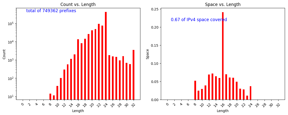
Figure 2: Prefix distribution in the U. of Oregon Route Views IPv4 table

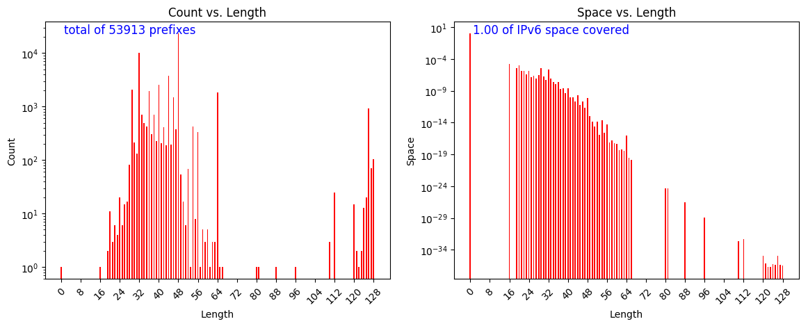
Figure 3: Prefix distribution in the U. of Oregon Route Views IPv6 table

In the absence of data on traffic patterns, we merely observe the effect of each synthetically generated pattern on the relative performance of the guided vs. linear search schemes. In all experiments, we use the balanced binary tree (equivalently, binary search) with the implication that prefix lengths in any one branch of the balanced tree are equally likely to match any one IP.

Figure 4: Balanced BST (used in experiments) vs. BST optimized exclusively for address share (not used), both based on the U. of Oregon Route Views IPv4 table

We also contrast the relative performance of the linear and guided search on IPv4 vs. IPv6 traffic. We use two traffic pattern extremes:

1. random traffic, where most if not all IPv6 queries go to default route;

2. traffic correlated with the frequency distribution of each prefix length (in the limit, using prefixes themselves as traffic).

Finally, we observe the effect of the BF hyperparameters: the bit vector size ($m$) – or equivalently, the percentage of bits set – and the count of hash functions ($k$) on the relative performance of the linear vs. guided search schemes.

TABLE I: Experiment Matrix

traffic	protocol
	IPv4	IPv6
random	✓	✓
by prefix address space	✓
by prefix frequency	✓	✓

4.2 Discussion

We summarize the results of the experiments with different IPv4 traffic types in Table II. For IPv4, the guided search requires about one half the number of accesses on a per packet basis compared to linear search.

TABLE II: IPv4 linear vs. guided search performance by traffic type; guided BF: $n=749362$ elements, $k=10$ hash funcs, $size=2.57$MB, $length=21548036$ bits, $33.3$% full; linear BF: $fpp=10^{-4}$, $n=749362$ elements, $k=14$ hash funcs, $size=1.71$MB, $length=14365358$ bits, $51.8$% full

traffic	metric (per packet)	linear	guided
random	bit lookup	49.3	22.1
	hashing	20.0	11.2
by prefix address space	bit lookup	48.0	22.3
	hashing	17.4	10.3
by prefix frequency	bit lookup	33.3	17.7
	hashing	10.3	8.6

Search performance vs. utilization ratio (% full) is documented in Table III. From Figure 5 it can be seen, that the linear vs. guided search relative performance levels off when the bitarray is approximately 10% full. For a table of approx. 750,000 entries, 10% full guided BF requires 10.3MB and can therefore fit in L3 cache on today’s general purpose CPUs. The performance for a compact 2.57MB guided BF is still an improvement over linear search, even though the search defaults to linear 68% of the time. The high default rate is reflected in the increased number of bit lookups and hash computations.

TABLE III: IPv4 guided search performance by utilization ratio (random traffic); guided BF: $n=749362$ elements, $k=10$ hash funcs

% bit vector full (size)	metric	count per packet
33.3% full (2.6MB)	bit lookup	22.1
	hashing	11.2
	FIB lookup	0.7
	default rate	68%
9.6% full (10.3MB)	bit lookup	14.0
	hashing	8.0
	FIB lookup	0.7
	default rate	30%
4.0% full (25.7MB)	bit lookup	12.5
	hashing	7.4
	FIB lookup	0.7
	default rate	22%

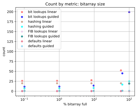
Figure 5: IPv4 search performance for guided vs. linear search; $n=749362$ elements, $k=10$ hash funcs

For IPv4, the number of bit lookups asymptotically approaches approximately eight per packet. With prefixes in the table covering approximately 67% of the address space, 33% of lookups will require four lookups to arrive at the default route, while the remaining 67% of lookups will traverse the full height of the balanced tree (five lookups), in addition to decoding the 5-bit best matching prefix sequence for a total of ten lookups. This calculation also suggests that $k=10$ hash functions is the minimum for the protocol to function.

Using the same assumption that the bit vector is sparse enough to never default to linear search, there would be just over five hash lookups per packet in the limit. Four hash computations are required to yield the default route for 33% of lookups and six hash computations are required for the remaining 67% of lookups, which includes five hashes to traverse the height of the tree and a single hash computation to decode the 5-bit sequence.

Last but not least, the proposed search algorithm is particularly effective for the IPv6 address space. This is to be expected with the 128-bit IP addresses that require only six bit vector lookups to match the default route with the logarithmic time complexity (Figure 6).

Figure 7 illustrates the relative performance of the two search algorithms for two IPv6 traffic patterns. At one extreme, there is the default-only traffic that is optimally suited for the guided search scheme. At the other extreme, there is the case of no-default traffic in direct proportion to the share of each prefix length (here we reuse prefixes as the traffic). For either traffic pattern, the guided scheme outperforms the linear search by an order of magnitude.

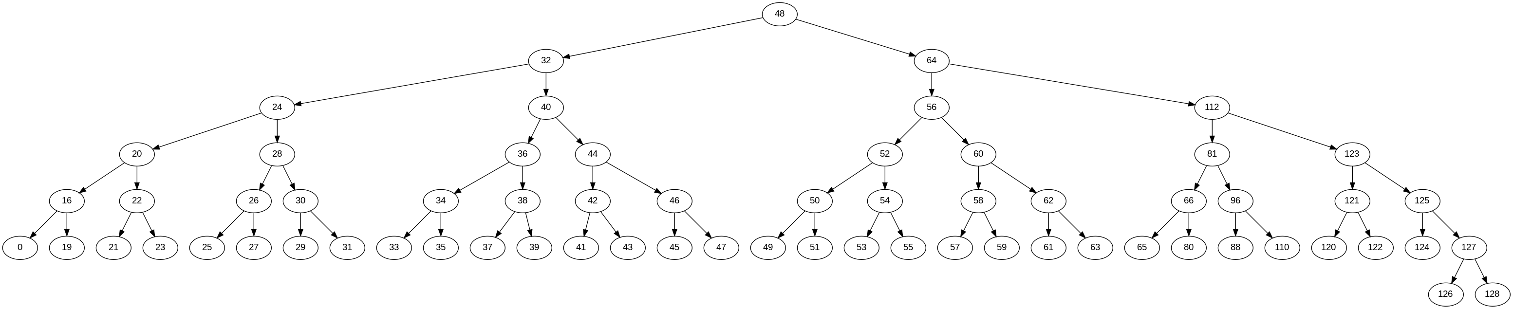
Figure 6: Binary search tree used for the IPv6 prefix search

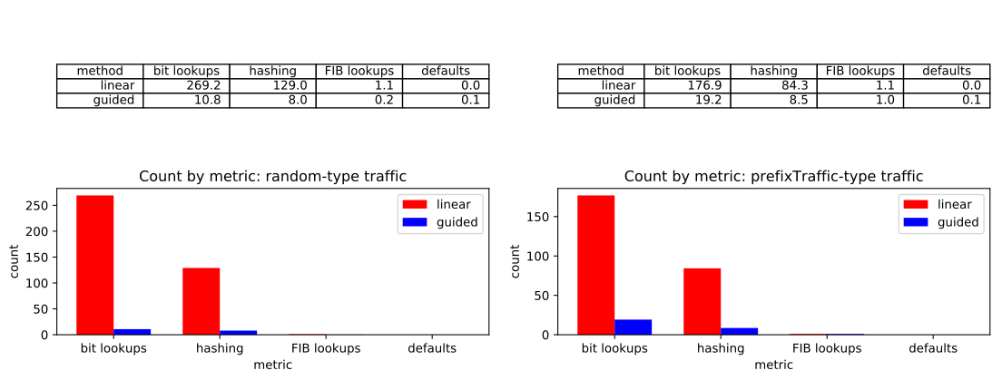
Figure 7: IPv6 search performance: random traffic that always defaults to 0-prefix length vs. traffic correlated with the share of each prefix length (no defaults); guided BF: $n=53913$ elements, $k=14$ hash funcs, $size=2.05$MB, $length=17238428$ bits, $4.4$% full; linear BF: $fpp=10^{-3}$, $n=53913$ elements, $k=10$, $size=0.09$MB, $length=775139$ bits, $50.1$% full

References

- [1] J. Kurose and K. Ross, Computer Networking: A Top-Down Approach, 6th ed. Addison Wesley, 2013.
- [2] M. A. Ruiz-Sanchez, E. W. Biersack, and W. Dabbous, “Survey and taxonomy of IP address lookup algorithms,” IEEE Network Magazine, vol. 15, no. 2, pp. 8–23, March 2001.
- [3] G. Varghese, Network Algorithmics. Morgan Kaufmann, 2007.
- [4] M. Waldvogel, G. Varghese, J. Turner, and B. Plattner, “Scalable high-speed IP routing lookups,” Proc. ACM SIGCOMM ’97 Conference on Applications, Technologies, Architectures, and Protocols for Computer Communication, pp. 25–38, October 1997.
- [5] S. Dharmapurikar, P. Krishnamurthy, and D. Taylor, “Longest prefix matching using Bloom filters,” IEEE/ACM Transactions on Networking, vol. 14, no. 2, pp. 397–409, April 2006.
- [6] M. Yegorov, “IP filter prototype,” https://github.com/myegorov/ip-filter/, 2018.
- [7] U. of Oregon, “Route Views Project,” http://bgp.potaroo.net/index-bgp.html, 2018, [Online; accessed 24-March-2018].