Optomechanical Entanglement of Remote Microwave Cavities

Abstract

We examine the entanglement properties of a system that represents two driven microwave cavities each optomechanically coupled to two separate driven optical cavities which are connected by a single-mode optical fiber. The results suggest that it may be possible to achieve near-maximal entanglement of the microwave cavities, thus allowing a teleportation scheme to enable interactions for hybrid quantum computing of superconducting qubits with optical interconnects.

I Introduction

Classical long-haul information networks utilize optical fibers for their low-loss and low-noise characteristics. Similarly, in the quantum regime, photons in optical fibers provide a proven and robust method to transmit quantum information reliably over long distances and at room temperature. Superconducting qubits, a leading candidate for a future quantum computer, operate in the microwave regime and must be cooled to milli-Kelvin temperatures for quantum operation. Off-chip connectivity at room temperature would be highly desirable in order to optically link superconducting chips. However, this requires a high-fidelity microwave-to-optical transducer that can be fiber-coupled into a quantum network.

The fundamental problem is then to convert a microwave qubit to an optical qubit, which was investigated via optomechanical resonators by Tian and Wang (2010); Stannigel et al. (2011); Tian (2012a); Barzanjeh et al. (2012); Clader (2014), and found to be feasible, while the concept of transferring states through optical connections in the presence of decoherence has been around for a while Pellizzari (1997); Cirac et al. (1997); van Enk et al. (1999); Serafini et al. (2006); Reiserer and Rempe (2015); Kurpiers et al. (2017); Axline et al. (2017).

The next stage of the problem is to couple two such optomechanical resonators by an optical fiber, as treated in Clader (2014) which showed that high-fidelity adiabatic state transfer is possible under realistic conditions, as did Yin et al. (2015).

A logical next step is to ask, can we achieve strong entanglement between optically networked microwave cavities, to use as a resource for quantum teleportation to improve state-transfer fidelity? Thus, the goal of the present work is to answer this question. While Tian (2013a) investigated the possibility of entangling two cavities connected by an optomechanical resonator, here we seek to entangle the two microwave cavities at either end of two different optomechanical resonators connected by an optical fiber, as seen in Fig.1 in Sec.II.

II Model

The overall model is 14 subsystems (modes) consisting of seven primary modes each individually coupled to one of seven noninteracting baths which are the secondary modes. Figure 1 depicts the total system.

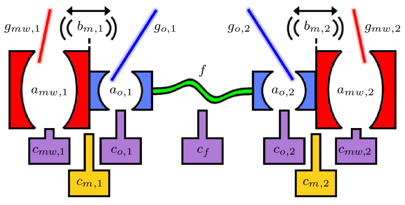
Figure 1: (color online) Two optomechanical oscillators each consisting of two laser-driven cavities coupled by a two-sided oscillating mirror, both connected by an optical fiber, and each primary subsystem coupled to its own isolated bath. Mode operators are shown near each component, and $g_{k}$ are driving laser strengths.

The linearized interaction-picture Hamiltonian is

$$H=H_{om,1}+H_{f}+H_{om,2}+H_{d},$$ (1)

where the time-dependence is suppressed, and where

$$\begin{array}[]{*{20}l}{H_{om,1}}&\!\!{=\hbar\left(\begin{array}[]{l}g_{mw,1}(a_{mw,1}^{{\dagger}}b_{m,1}+a_{mw,1}b_{m,1}^{{\dagger}})\\ +g_{o,1}(a_{o,1}^{{\dagger}}b_{m,1}+a_{o,1}b_{m,1}^{{\dagger}})\\ \end{array}\right)}\\ {H_{om,2}}&\!\!{=\hbar\left(\begin{array}[]{l}g_{o,2}(a_{o,2}^{{\dagger}}b_{m,2}+a_{o,2}b_{m,2}^{{\dagger}})\\ +g_{mw,2}(a_{mw,2}b_{m,2}+a_{mw,2}^{{\dagger}}b_{m,2}^{{\dagger}})\\ \end{array}\right)\!,}\\ \end{array}$$ (2)

are the optomechanical terms where the beam-splitter terms of the form $\hbar g(a^{{\dagger}}b+ab^{{\dagger}})$ correspond to cavities driven in the “low sideband,” meaning that the driving lasers are detuned below the cavity resonance frequency with detuning $\Delta\equiv\omega_{L}-\omega_{c}\approx-\omega_{m}$ where $\omega_{L}$ is the laser field’s angular frequency, $\omega_{c}$ is the resonsant angular frequency of the cavity being driven, and $\omega_{m}$ is the resonant angular frequency of the mechanical oscillator of the local optomechanical system (two cavities coupled by a moveable two-sided mirror). The term with form $\hbar g(ab+a^{{\dagger}}b^{{\dagger}})$ is a two-mode squeezing Hamiltonian corresponding to driving in the “high sideband,” meaning that the second microwave cavity’s driving laser is detuned above the cavity resonance frequency as $\Delta\equiv\omega_{L}-\omega_{c}\approx+\omega_{m}$. Thus we call this the “LLLH model” since three cavities are driven low, and the one at the end is driven high.

The reason for driving one of the four cavities in the high sideband is that if our goal is to generate two-mode squeezing between the two microwave cavities, then we want to achieve the Bogoliubov modes, which are Tian (2013a)

$$\begin{array}[]{*{20}l}{\beta_{1}}&\!\!{=\cosh(r)a_{mw,1}+i\sinh(r)a_{mw,2}^{{\dagger}}}\\ {\beta_{2}^{{\dagger}}}&\!\!{=-i\sinh(r)a_{mw,1}+\cosh(r)a_{mw,2}^{{\dagger}},}\\ \end{array}$$ (3)

which lead to two-mode squeezing on the vacuum, where $r\in[0,\infty)$ is the squeezing parameter. The fact that the Bogoliubov modes are combinations of annihilation and creation operators means that the cavities being squeezed must have opposite sideband driving, and it was found that such modes only emerged when the other two cavities were driven in the low sideband.

The single-mode optical fiber’s lone Hamiltonian is

$$H_{f}=\hbar g_{f}((a_{o,1}-a_{o,2})f^{{\dagger}}+(a_{o,1}^{{\dagger}}-a_{o,2}^{{\dagger}})f),$$ (4)

and the dissipation term is

$$\begin{array}[]{*{20}l}{H_{d}=}&\!\!{H_{do,1}+H_{dm,1}+H_{dmw,1}+H_{d{\kern 0.1pt}f}}\\ {}&\!\!{+H_{do,2}+H_{dm,2}+H_{dmw,2},}\\ \end{array}$$ (5)

where each of these terms has the form

$$\begin{array}[]{*{20}l}{H_{dk}(t)=}&\!\!{\hbar\int_{-\infty}^{\infty}{(\omega-\omega_{k})c_{k}^{{\dagger}}(\omega,t)c_{k}(\omega,t)d\omega}}\\ {}&\!\!{+i\hbar\int_{-\infty}^{\infty}{g_{dk}(a_{k}^{{\dagger}}(t)c_{k}(\omega,t)-a_{k}(t)c_{k}^{{\dagger}}(\omega,t))d\omega}},\\ \end{array}$$ (6)

where the fact that coupling strengths $g_{dk}$ are shown as frequency-independent is the “first Markov approximation,” and this form is the result of the rotating wave approximation (RWA). Note that in (6), $a$ is an abbreviation for all main-system annihilation (mode) operators, and $k$ is a general index that can take on any label of each subsystem, and where the ordering of these labels will be defined in Sec.II.1. Also note that Gardiner and Collett (1985) specifies the opposite order of terms in the second large term of (6), likely because the naming convention in Tian (2013a) caused an exchange of terms, leading to an apparently unimportant sign-flip in the coupling strengths of the baths. We leave it here, as in Clader (2014), for consistency with Tian (2013a).

II.1 Langevin Equation and Solution

The Langevin equation for this system is

$$i{\textstyle{{d\mathbf{v}(t)}\over{dt}}}=M(t)\mathbf{v}(t)+i\sqrt{K}\mathbf{v}_{\text{in}}(t),$$ (7)

as derived in App.A, where, suppressing time,

$${\!\!}\begin{array}[]{*{20}l}{\mathbf{v}}&\!\!\!{\equiv\!(a_{o,1},b_{m,1},a_{mw,1},f,a_{o,2},b_{m,2},a_{mw,2}^{{\dagger}})^{T}}\\ {\mathbf{v}_{\text{in}}}&\!\!\!{\equiv\!(a_{o,1,\text{in}},b_{m,1,\text{in}},a_{mw,1,\text{in}},f,a_{o,2,\text{in}},b_{m,2,\text{in}},a_{mw,2,\text{in}}^{{\dagger}})^{T}\!\!\!\!,}\\ \end{array}$$ (8)

and the diagonal damping matrix is

$$K\equiv{\textstyle{1\over{2\pi}}}\text{diag}(\begin{array}[]{*{20}c}{\kappa_{o,1}}&{\kappa_{m,1}}&{\kappa_{mw,1}}&{\kappa_{f}}&{\kappa_{o,2}}&{\kappa_{m,2}}&{\kappa_{mw,2}}\\ \end{array}),$$ (9)

and the time-dependent dynamics matrix is

$$M{\kern-1.5pt}\equiv{\kern-4.0pt}\left(\!\!{\begin{array}[]{*{20}c}{{\textstyle{{-i\kappa_{o,1}}\over 2}}}&\!\!\!{g_{o,1}}&\!\!\!\cdot&\!\!\!{g_{f}}&\!\!\!\cdot&\!\!\!\cdot&\!\!\!\cdot\\ {g_{o,1}}&\!\!\!{{\textstyle{{-i\kappa_{m,1}}\over 2}}}&\!\!\!{g_{mw,1}}&\!\!\!\cdot&\!\!\!\cdot&\!\!\!\cdot&\!\!\!\cdot\\ \cdot&\!\!\!{g_{mw,1}}&\!\!\!{{\textstyle{{-i\kappa_{mw,1}}\over 2}}}&\!\!\!\cdot&\!\!\!\cdot&\!\!\!\cdot&\!\!\!\cdot\\ {g_{f}}&\!\!\!\cdot&\!\!\!\cdot&\!\!\!{{\textstyle{{-i\kappa_{f}}\over 2}}}&\!\!\!{-g_{f}}&\!\!\!\cdot&\!\!\!\cdot\\ \cdot&\!\!\!\cdot&\!\!\!\cdot&\!\!\!{-g_{f}}&\!\!\!{{\textstyle{{-i\kappa_{o,2}}\over 2}}}&\!\!\!{g_{o,2}}&\!\!\!\cdot\\ \cdot&\!\!\!\cdot&\!\!\!\cdot&\!\!\!\cdot&\!\!\!{g_{o,2}}&\!\!\!{{\textstyle{{-i\kappa_{m,2}}\over 2}}}&\!\!\!{g_{mw,2}}\\ \cdot&\!\!\!\cdot&\!\!\!\cdot&\!\!\!\cdot&\!\!\!\cdot&\!\!\!{-g_{mw,2}}&\!\!\!{{\textstyle{{-i\kappa_{mw,2}}\over 2}}}\\ \end{array}}\!\!\right){\kern-2.5pt},$$ (10)

where the dots represent zeros, and we suppressed the time-dependence in $M$ and the driving-laser strengths $g_{mw,1}$, $g_{mw,2}$, $g_{o,1}$, $g_{o,2}$, and the damping strengths are $\kappa_{k}\equiv 2\pi g_{dk}^{2}$. The order of the subsystems was chosen to give $M$ as close to a block-diagonal form as possible.

The solution to the Langevin equation in (7) is

$$\mathbf{v}(t)=\tau(t,0)\mathbf{v}(0)+\int_{0}^{t}{\tau(t,t^{\prime})\sqrt{K}\mathbf{v}_{\text{in}}(t^{\prime})}dt^{\prime},$$ (11)

where $\tau(t,t^{\prime})$ is the propagator

$$\tau(t,t^{\prime})\equiv\tau\left\{{e^{-i\int_{t^{\prime}}^{t}{M(t^{\prime\prime})dt^{\prime\prime}}}}\right\},$$ (12)

where $\tau\{\cdot\}$ is the time-ordering operator.

II.2 Determination of Parameter Values and Pre-Optimization

There are several preliminary steps to take before looking at entanglement. First, we have to find a set of physically realistic starting values for the parameters of the problem. Then we have to look for nearby combinations of these values for which the Routh-Hurwitz (RH) stability conditions are satisfied DeJesus (1987) for the numerical stability of the model. We also need to make sure that the $\kappa/g$ ratios are all above the quoted physically achievable minima. We call this part “pre-optimization.” Then we can calibrate the program and be ready to look for regions of entanglement.

II.2.1 Initial Parameter Values

Our starting values are summarized in Table 1, with unenhanced laser-coupling strength $g_{0}=5.65\times 10^{6}\,[{\textstyle{{\text{rad}}\over\text{s}}}]$.

Table 1: Initial parameter values, explained in App.B.

Type $k$	$\kappa_{k}$ $[{\frac{\text{rad}}{\text{s}}}]$	$g_{k}$ $[{\frac{\text{rad}}{\text{s}}}]$
$mw$	$5.65\times 10^{5}$	$5.65\times 10^{6}$
$o$	$3.77\times 10^{5}$	$7.53\times 10^{5}$
$m$	$1.88\times 10^{3}$	$5.65\times 10^{6}$
$f$	$6.27\times 10^{8}$	$2.67\times 10^{9}$

From Tian (2013a), the achievable minimum $\kappa/g$ ratios are

$$({\textstyle{{\kappa_{mw}}\over{g_{mw}}}})_{\text{min}}{\kern-1.0pt}={\kern-1.0pt}0.1,\;\;\;({\textstyle{{\kappa_{o}}\over{g_{o}}}})_{\text{min}}{\kern-1.0pt}={\kern-1.0pt}0.5,\;\;\;({\textstyle{{\kappa_{m}}\over{g_{m}}}})_{\text{min}}{\kern-1.0pt}={\kern-1.0pt}3.33\times{\kern-2.0pt}10^{-4}{\kern-2.0pt}.$$ (13)

These ratios are the minimum amount of damping per driving strength reported as achievable, and represent how well these objects can dissipate energy that is pumped into them without catastrophic failure.

II.2.2 Routh-Hurwitz Stability Conditions

From DeJesus (1987), if we recast the Langevin equation as

$${\textstyle{{d\mathbf{v}(t)}\over{dt}}}=H(t)\mathbf{v}(t)+\sqrt{K}\mathbf{v}_{\text{in}}(t),$$ (14)

where $H\!\equiv\!-iM$, then the system is Routh-Hurwitz (RH) stable if all the real parts of the eigenvalues of $H$ are negative. Thus, a good metric for RH stability is

$$S_{\text{RH}}\equiv\text{max}(\text{Re}(\text{eig}(H))),$$ (15)

where $S_{\text{RH}}<0$ is the necessary and sufficient condition for RH stability. Note that $S_{\text{RH}}=0$ is an indeterminate case, which is not necessarily stable or unstable.

Minimizing $S_{\text{RH}}$ over all parameter combinations is the main objective of our pre-optimization; basically we want to find a possibly new set of initial parameter values that are RH stable. However, these values also need to have physically achievable $\kappa/g$ ratios.

II.2.3 Physical Parameter Assignment

Before we can start the pre-optimization, we have to connect the theoretical parameters to the physical parameters. Since we want to generate two-mode squeezing between the microwave cavities, a first guess for achieving this is to choose the assignment

$$\begin{array}[]{*{20}l}{g_{mw,1}=g_{0}\cosh(r),}&{g_{o,1}\in[g_{0},100g_{0}],}\\ {g_{mw,2}=g_{0}\sinh(r),}&{g_{o,2}\in[g_{0},100g_{0}].}\\ \end{array}$$ (16)

Then, we could express the Bogoliubov modes as linear combinations of the cavity modes where the coefficients are proportional to the driving laser strengths as

$$\begin{array}[]{*{20}l}{\beta_{1}}&\!\!{={\textstyle{1\over{g_{0}}}}(g_{mw,1}a_{1}+ig_{mw,2}a_{2}^{{\dagger}})}\\ {\beta_{2}^{{\dagger}}}&\!\!{={\textstyle{1\over{g_{0}}}}(-ig_{mw,2}a_{1}+g_{mw,1}a_{2}^{{\dagger}}),}\\ \end{array}$$ (17)

where the squeezing parameter is then

$$r=\tanh^{-1}({\textstyle{{g_{mw,2}}\over{g_{mw,1}}}}).$$ (18)

Of course many other assignments are possible, so the choice in (16) may not be the most effective, but it is a convenient starting place for further investigations.

II.2.4 Choice of Target Squeezing Parameter

Since the logarithmic negativity $E_{\mathcal{N}}$ Vidal and Werner (2002), the entanglement measure we use in Sec.II.3, has range $E_{\mathcal{N}}\in[0,\infty)$ for infinite-level systems, we need to know what value is “high enough” for near-maximal entanglement.

From Hedemann (2014, 2018), a properly normalized multipartite entanglement monotone is the ent, which for a two-mode squeezed state with squeezing parameter $r\in[0,\infty)$ is

$$\Upsilon(r)=1-{\textstyle{1\over{2\cosh^{2}(r)-1}}}\in[0,1],$$ (19)

where $\Upsilon(0)=0$ corresponds to the separable two-mode vacuum state, and the value of $\Upsilon(\infty)=1$ is for the maximally entangled two-mode squeezed state; see App.C.

Though our two cavities are not an isolated system, focusing on them effectively traces over the rest of the system, and (19) acts as a mathematical lens for viewing how good the squeezing parameter would be if the system were isolated and started from vacuum. Thus, we can specify any target ent $\Upsilon_{\ast}\in[0,1]$ that we want, and obtain a target ideal squeezing parameter $r_{\ast}$ from

$$r_{\ast}(\Upsilon_{{\ast}})=\cosh^{-1}\left({\sqrt{{\textstyle{1\over 2}}({\textstyle{1\over{1-\Upsilon_{\ast}}}}+1)}}\right).$$ (20)

For example, if we want an ent of $\Upsilon_{\ast}=0.999$, (20) yields

$$r_{\ast}(0.999)\approx 3.8,$$ (21)

which shows that a relatively low value of $r$ is sufficient for near-maximal entanglement of the reduced system of the cavities, assuming that the modes evaluated for entanglement are Bogoliubov modes, even if momentarily.

II.2.5 Pre-Optimization Results

Pre-optimization seeks a “winning” parameter-value combination $\mathbf{g}\equiv(g_{mw,1},g_{mw,2},g_{o,1},g_{o,2})$ (where the functional definitions of its elements would change if we choose a different physical parameter assignment than that in (16)), such that the RH metric of (15) satisfies $S_{\text{RH}}<0$, while the $\kappa/g$ ratios are all kept above the achievable minima in (13), and we try to keep squeezing parameter $r$ as high as possible, meaning $r\geq 3.8$, the “good enough” value from (21). The purpose of pre-optimization is to show that parameter combinations exist that can satisfy all the desired constraints, which in our case are indepedent of the solution to the Langevin equation (though they can still depend on time).

As a first iteration, the values of Table 1 were used for a static-driving-laser snapshot of the RH stability, using $r=3.8$. Then, the damping strengths $\kappa$ were increased manually (permissible since that simply implies that we make more heavily damped cavities) while increasing $r$ and checking the $\kappa/g$ ratios against (13). This resulted in new damping values,

$$\kappa_{mw}=20C,\;\;\;\kappa_{o}=60C,\;\;\;\kappa_{m}=0.001C,$$ (22)

where $C$ is given in (55), and increased squeezing parameter $r=3.85$. The optical damping was then further adjusted as

$$\kappa_{o,1}=\kappa_{o},\;\;\;\kappa_{o,2}=2.5\kappa_{o},$$ (23)

to keep all $\kappa/g$ ratios above their minima. Figure 2 shows the RH metric tested over this parameter set.

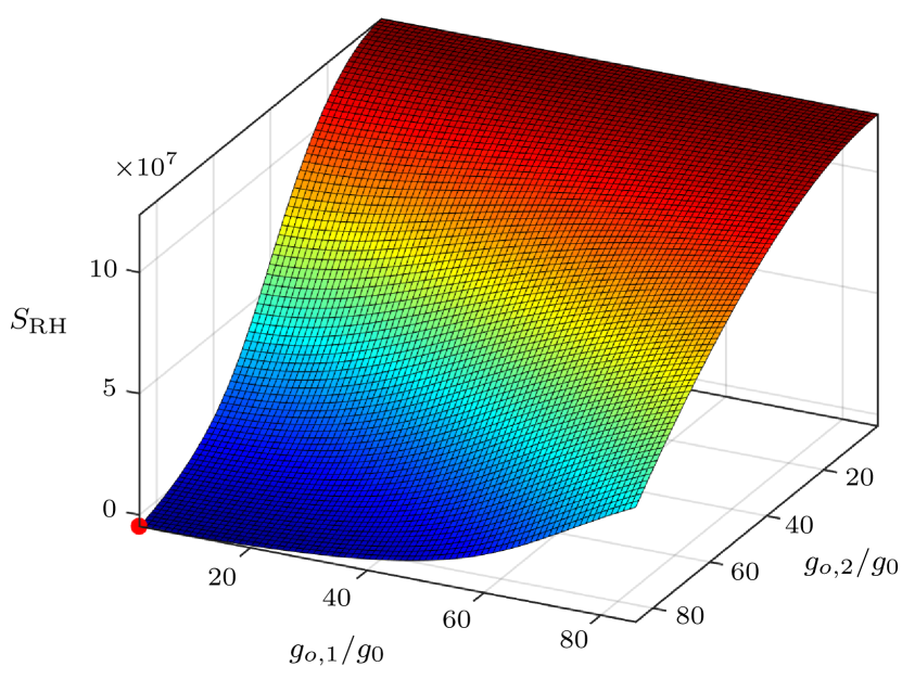
Figure 2: (color online) Plot of RH metric $S_{\text{RH}}(H)$ from (15), where $H\equiv-iM$, where $M$ is given in (10), and we use only fixed parameter values here, as mentioned in the text. The surface shows RH-stability metric $S_{\text{RH}}$ for all parameter combinations tested, and the red dot is the winner $\min(S_{\text{RH}})$. All nonlaser parameters were held constant, with $r=3.85$.

The $\kappa/g$ ratios for this parameter set were

$$\begin{array}[]{*{20}l}{{\textstyle{{\kappa_{mw,1}}\over{g_{mw,1}}}}=0.284,}&{{\textstyle{{\kappa_{o,1}}\over{g_{o,1}}}}=20.0,}&{{\textstyle{{\kappa_{m,1}}\over{g_{m,1}}}}=3.33\times 10^{-4},}\\[8.0pt] {{\textstyle{{\kappa_{mw,2}}\over{g_{mw,2}}}}=0.284,}&{{\textstyle{{\kappa_{o,2}}\over{g_{o,2}}}}=0.581,}&{{\textstyle{{\kappa_{f}}\over{g_{f}}}}{\kern 8.0pt}=0.236,}\\ \end{array}$$ (24)

which shows that we have found physically achievable $\kappa/g$ ratios while also attaining the “good” squeezing parameter $r=3.85$, and the safely negative RH-metric value,

$$\min(S_{\text{RH}})=-4.75\times 10^{6}\ll 0.$$ (25)

Note that finding a valid parameter combination with a “good” $r$ does not mean that cavities have the entanglement corresponding to $r$; rather it means that in the reference frame of the Bogoliubov modes, the system behaves as a two-mode squeezed state with that $r$. If at any times the time-dependent cavity modes are equal to those Bogoliubov modes, then their entanglement will reach that value at those instances.

In fact, we found that it was possible to construct the Bogoliubov modes from linear combinations of the eigenmodes of $H$, numerically verified to 15 decimal places, even with damping. Therefore, near-maximal entanglement is possible in this system. However, the expressions are highly nonlinear and transcendental, making it infeasible to analytically obtain the conditions for instances of Bogoliubov modes, as was done in Tian (2013a). Therefore we must use numerical methods here.

Now we are ready to construct an optimization that includes all of these features, including entanglement, which we develop next.

II.3 Entanglement Calculation

As explained in detail in App.D, the entanglement of the two micrwoave cavities as logarithmic negativity is

$$E_{\mathcal{N}}=\max\{0,-\log_{2}(2r_{0})\},$$ (26)

where

$$r_{0}=\sqrt{{\textstyle{{b-\sqrt{b^{2}-4c}}\over 2}}},$$ (27)

with scalars

$$b=\det(A)+\det(B)-2\det(C)\;\;\;\text{and}\;\;\;c=\det(V),$$ (28)

where $V$ is the covariance matrix,

$$V=\left({\begin{array}[]{*{20}c}A&C\\ {C^{T}}&B\\ \end{array}}\right),$$ (29)

with marginal block-matrices

$$A=(\langle a_{1}^{{\dagger}}a_{1}\rangle+{\textstyle{1\over 2}})\left({\begin{array}[]{*{20}c}1&0\\ 0&1\\ \end{array}}\right)\!,\;\;B=(\langle a_{2}^{{\dagger}}a_{2}\rangle+{\textstyle{1\over 2}})\left({\begin{array}[]{*{20}c}1&0\\ 0&1\\ \end{array}}\right)\!,$$ (30)

and correlation block matrix,

$$C=\left({\begin{array}[]{*{20}r}{{\textstyle{1\over 2}}(\langle a_{1}a_{2}\rangle+\langle a_{1}^{{\dagger}}a_{2}^{{\dagger}}\rangle)}&{{\textstyle{1\over{2i}}}(\langle a_{1}a_{2}\rangle-\langle a_{1}^{{\dagger}}a_{2}^{{\dagger}}\rangle)}\\ {{\textstyle{1\over{2i}}}(\langle a_{1}a_{2}\rangle-\langle a_{1}^{{\dagger}}a_{2}^{{\dagger}}\rangle)}&{-{\textstyle{1\over 2}}(\langle a_{1}a_{2}\rangle+\langle a_{1}^{{\dagger}}a_{2}^{{\dagger}}\rangle)}\\ \end{array}}\right)\!,$$ (31)

(not to be confused with the scalar $C$ in (22)) where the time-dependent expectation-value functions are given in App.D in (71–74).

For reference, the logarithmic negativity in terms of the ideal squeezing parameter $r_{*}$ and ideal ent $\Upsilon_{*}$ is

$$E_{\mathcal{N}}={\textstyle{{1}\over{\ln(\sqrt{2})}}}r_{*}={\textstyle{{1}\over{\ln(\sqrt{2})}}}\cosh^{-1}\!\left({\sqrt{{\textstyle{1\over 2}}({\textstyle{1\over{1-\Upsilon_{\ast}}}}+1)}}\right),$$ (32)

where the term ideal refers to what these quantities would mean if the two microwave cavities were in an isolated two-mode squeezed state Hedemann (2018).

III Results and Optimization of Entanglement

Here we present the results of several types of searches for near-maximal entanglement of the driven cavities. Due to the combinatorially-hard nature of this problem, these results are by no means exhaustive, yet they demonstrate that it should be possible to achieve entanglement as a resource for quantum teleportation between remote microwave cavities with optical fiber connections.

III.1 Numerical Optimization of Entanglement

The highest entanglement found from search-based optimization was achieved by abandoning the notion of hyperbolically fixing two of the driving lasers (as in (16)), and instead allowing all four driving lasers to be pulse shapes with all parameters allowed to roam within certain domains, tested over many iterations and fueled by a pseudo-random number generator.

The pulses were doubly-asymmetric trapezoidal functions, where starting height, peak height, and end heights could all be different, as well as start time, rise time, peak width, and fall time, and the starting height was constrained to be zero. Figure 3 shows the results of the search for a parameter combination that caused an instant of highest logarithmic negativity such that all time points were RH-stable, and all $\kappa/g$ ratios were within an order of magnitude of the achievable minima.

The peak entanglement in Fig.3 is

$$\text{max}(E_{\mathcal{N}})=3.49,\;\;\;\text{max}(\Upsilon)=0.823,$$ (33)

which is comparable to $\text{max}(E_{\mathcal{N}})\approx 3.45$ derived analytically in Tian (2013a) for the simpler system of two mechanically coupled cavities. Here, in the zero-damping limit, we get $\text{max}(\Upsilon)=0.939$, though in that case the stability is indeterminate without the damping to act as ballast.

The damping used in Fig.3 is

$$\kappa_{mw}=0.8C,\;\;\;\kappa_{o}=0.9C,\;\;\;\kappa_{m}=0.001C,$$ (34)

however, the search method used the zero-damping case to switch-off unnecessary expressions to pre-screen for quasi-stable results at higher speed, using the low positive threshold $S_{\text{RH}}<10^{-4}$ instead of the proper condition $S_{\text{RH}}<0$. Then the candidate pulse sets were applied to the damped system with the correct stability condition, and the pulse set with the highest peak $E_{\mathcal{N}}$ was the winning set, as seen in Fig.3b.

The minimum $\kappa/g$ ratios achieved in Fig.3 are

$$\begin{array}[]{*{20}l}{\min({\textstyle{{\kappa_{mw,1}}\over{g_{mw,1}}}})}&\!\!{=2.86\times 10^{-3}}&\;\;{\min({\textstyle{{\kappa_{o,1}}\over{g_{o,1}}}})}&\!\!{=6.66\times 10^{-3}}\\[8.0pt] {\min({\textstyle{{\kappa_{mw,2}}\over{g_{mw,2}}}})}&\!\!{=7.22\times 10^{-3}}&\;\;{\min({\textstyle{{\kappa_{o,2}}\over{g_{o,2}}}})}&\!\!{=4.67\times 10^{-3},}\\ \end{array}$$ (35)

which are two orders of magnitude less than the minimum achievable values of (13). However, these mimima only need to be attained briefly ($50\,[\text{ns}]$), and therefore this may be an achievable regime now or in the near future.

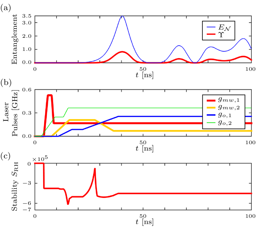
Figure 3: (color online) Random-search-based winner over sets of four trapezoidal pulses. (a) Entanglement as logarithmic negativity $E_{\mathcal{N}}\in[0,\infty)$ and ent $\Upsilon\in[0,1]$. (b) Driving-laser pulses. (c) RH-stability metric $S_{\text{RH}}$. Trapezoidal-rule step number was $n=5$, and propagator step number was $N=50$ for computational efficiency ($n=10$ and $N=1600$ are best for convergence, but the difference is negligible); see App.F. All subsystems were in the vacuum state initially, and $1000$ time points were used, connected by line segments here and in later plots, though keep in mind that may not be the “truth.”

So far, we have modeled everything as starting in the vacuum state, but if we model the mechanical oscillators’ baths as being initially in states with mean thermal occupation numbers $N_{\text{th}}$, the entanglement drops further, as seen in Fig.4.

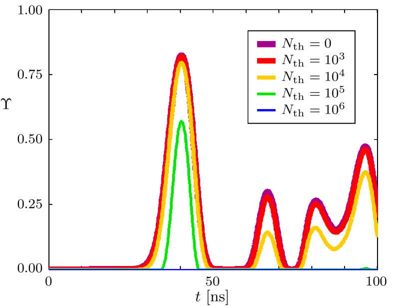
Figure 4: (color online) Ent values of the damped system from Fig.3, shown here for various values of thermal occupation number $N_{\text{th}}$ for the mechanical oscillator baths. The peak ent is $0.823$ for $N_{\text{th}}=0$, and remains near this until $N_{\text{th}}=10^{3}$, after which it dies to zero near $N_{\text{th}}=10^{6}$.

As Fig.4 shows, the entanglement of the damped microwave cavities is fairly robust against mechanical oscillator noise up to about $N_{\text{th}}=10^{3}$. Note that since stability $S_{\text{RH}}$ depends on $H$, it is independent of $N_{\text{th}}$.

III.2 Frequency-Filtered Entanglement Optimization

An alternative way to study entanglement in this system is to look at the effect of operating the system only in a narrow band of frequencies, meaning that the solution to the Langevin equation is filtered to only allow Fourier components from a narrow frequency band.

Using only constant laser driving strengths, the solution to the frequency-filtered Langevin equation is

$$\mathbf{v}^{\prime}_{\text{out}}(\omega_{n})=S(\omega_{n})\mathbf{v}^{\prime}_{\text{in}}(\omega_{n}),$$ (36)

where $\omega_{n}\equiv n\Delta\omega$ is a discrete set of (angular) frequencies such that $n$ is an integer and $\Delta\omega$ is a narrow frequency window, and $S\equiv S(\omega)$ is the transfer matrix

$$S(\omega)\equiv I-i\sqrt{K}(\omega I-M)^{-1}\sqrt{K}.$$ (37)

The elements of $\mathbf{v}^{\prime}_{\text{out}}(\omega_{n})$ and $\mathbf{v}^{\prime}_{\text{in}}(\omega_{n})$ in (36) are annihilation and creation operators that are summations over mode operators of all possible frequencies weighted by a band-pass filtering function, as described in App.E.

To attempt to optimize the frequency-filtered solution, we performed a random search of $10^{5}$ trials producing sets of random driving-laser strengths $g_{k}\in[0,110g_{0}]$, and designated the winning set as the one that produced the largest peak $E_{\mathcal{N}}$ while producing $S_{\text{RH}}<0$ for RH-stability. The result is shown in Fig.5.

Figure 5: (color online) Ent values for the frequency-filtered damped system for a range of different angular frequency windows $\omega_{n}$. The peak ent is 0.839 for $N_{\text{th}}=0$, and like Fig.4, remains near this through $N_{\text{th}}=10^{3}$, but decreases more slowly with $N_{\text{th}}$. For all curves, $S_{\text{RH}}=-3.80\times 10^{5}$.

The damping in Fig.5 is that of (34), and the winning $g_{k}$ values that produced Fig.5 are

$$\begin{array}[]{*{20}l}{g_{mw,1}=121.9\;[\text{MHz}],}&{g_{o,1}=605.4\;[\text{MHz}],}\\ {g_{mw,2}=105.5\;[\text{MHz}],}&{g_{o,2}=549.6\;[\text{MHz}],}\\ \end{array}$$ (38)

so the $\kappa/g$ ratios are

$$\begin{array}[]{*{20}l}{{\textstyle{{\kappa_{mw,1}}\over{g_{mw,1}}}}}&\!\!{=1.234\times 10^{-2}\!,}&\;\;{{\textstyle{{\kappa_{o,1}}\over{g_{o,1}}}}}&\!\!{=2.795\times 10^{-3}\!,}\\[8.0pt] {{\textstyle{{\kappa_{mw,2}}\over{g_{mw,2}}}}}&\!\!{=1.426\times 10^{-2}\!,}&\;\;{{\textstyle{{\kappa_{o,2}}\over{g_{o,2}}}}}&\!\!{=3.079\times 10^{-3}\!,}\\ \end{array}$$ (39)

which are all about one order of magnitude less than the minimum achievable values of (13), which again, may be within the realm of possibility.

Thus, frequency-filtering this system can achieve near-maximal entanglement while maintaining RH-stability.

IV Conclusions

We have derived and explored the entanglement properties of a nonadiabatic linearized quantum-mechanical model of two laser-driven optomechanical systems (each consisting of one microwave cavity and one optical cavity coupled by a two-sided mirror acting as a mechanical oscillator) coupled by a short single-mode optical fiber connected to the optical cavities.

In particular, we explored this system’s ability to achieve and maintain high levels of entanglement between the microwave cavities. The purpose of this is to enable a continuous-variable quantum teleportation scheme for ideal state transfer between microwave cavities, the intended application being a distributed superconducting-qubit architecture to improve the scalability of superconducting-qubit quantum computers.

Since this system is large enough to contain a computationally difficult number of parameters, we approached the entanglement optimization numerically from several different perspectives.

First, Sec.III.1 did a random search of parameters describing a set of four general trapezoidal laser pulses, where the starting height was constrained to zero, but the ending height was allowed to be larger than the central height. This method also pre-screened its candidates based on their approximate Routh-Hurwitz- (RH)-stability properties as calculated in the zero-damping regime, before evaluating the passing candidates in the damping regime. This method provided us with the result in Fig.3 that shows a decent level of entanglement, nearly exactly the same as was found in Tian (2013a) analytically, while also maintaining RH-stability. The downsides to this were that the entanglement only lasts on the order of ns, and it required $\kappa/g$ ratios that were two orders of magnitude lower than known-achievable values. However, one positive aspect of this example is its robustness against thermal noise, as seen in Fig.4 showing that the entanglement stays approximately unchanged for mean thermal occupation numbers up to $N_{\text{th}}=10^{3}$ for the baths of the mechanical oscillators.

Finally, Sec.III.2 examined a frequency-filtered model, similar to that in Tian (2013a). This method uses constant laser pulses and looks at only a narrow band of operating frequencies of the solution of equation of motion (the Langevin equation). The method was a random numerical search over the four laser pulse strengths, looking for the set that caused the highest peak entanglement while maintaining RH-stability. The winning result over $10^{5}$ trials produced a value only sightly higher than that found in Sec.III.1, and the system again showed the same robustness against thermal noise up to $N_{\text{th}}=10^{3}$. While the results in Tian (2013a) show a much higher peak entanglement, examination of its methods in Tian (2013b) shows a disagreement between our derivations, since there, the Langevin equation is first adiabatically approximated but then the input-output relation is omitted, whereas here we did not make the adiabatic approximation and used the input-output relation. Therefore the qualitative differences in the results may be due to a derivation error in one of these methods, or possibly they arise from using different approximations.

Since the writing of this paper began, several advances have been made in similar areas in Chen et al. (2014); Abdi et al. (2014, 2015); Ma and Wu (2015); Černotík and Hammerer (2016), though each for a slightly different system, and with different approaches. Recently, others have explored alternative control methods, such as Stefanatos (2017) where cavity coupling strengths are modulated. Perhaps similar variations may help future investigations to surpass our results.

Ultimately, the main results of this work are that this kind of interconnected driven quantum system is capable of achieving significant levels of entanglement for fairly decent amounts of time, which may enable teleportation schemes Braunstein and van Loock (2005) to accomplish high-fidelity state transfer between remote microwave cavities connected via optical fibers. Our results suggest that distributed superconducting quantum computing may be feasible, particularly if damping-to-driving-strength ratios can be lowered.

Appendix A Derivation of the Langevin Equation

The Heisenberg equations for the bath operators are

$${\textstyle{{dc_{k}(\omega,t)}\over{dt}}}=i[{\textstyle{1\over\hbar}}H(t),c_{k}(\omega,t)]=i[{\textstyle{1\over\hbar}}H_{dk}(t),c_{k}(\omega,t)],$$ (40)

where the bath operators obey

$$[c_{j}(\omega,t),c_{k}^{{\dagger}}(\omega^{\prime},t)]=\delta_{j,k}\delta(\omega-\omega^{\prime}).$$ (41)

Then putting (6) and (41) into (40) yields

$$i{\textstyle{{dc_{k}(\omega,t)}\over{dt}}}=(\omega-\omega_{k})c_{k}(\omega,t)-ig_{dk}a_{k}(t),$$ (42)

where we used the bosonic commutation relations $[a_{j},a_{k}^{{\dagger}}]=\delta_{j,k}$ for the primary mode operators. Direct integration of (42) gives solutions

$$\begin{array}[]{*{20}l}{c_{k}(\omega,t)=}&\!\!{e^{-i(\omega-\omega_{k})(t-t_{0})}c_{k}(\omega,t_{0})}\\ {}&\!\!{-g_{dk}\int_{t_{0}}^{t}{a_{k}(t^{\prime})e^{-i(\omega-\omega_{k})\left({t-t^{\prime}}\right)}dt^{\prime}.}}\\ \end{array}$$ (43)

The Heisenberg equations for the primary modes are

$${\textstyle{{da_{k}(t)}\over{dt}}}=i[{\textstyle{1\over\hbar}}H(t),a_{k}(t)],$$ (44)

and putting (1) into (44) gives

$${\kern-1.0pt}\begin{array}[]{*{20}l}{i{\textstyle{{da_{o,1}}\over{dt}}}}&\!\!{=g_{o,1}b_{m,1}+g_{f}f+i\int_{-\infty}^{\infty}{}g_{do,1}c_{o,1}(\omega,t)d\omega}\\ {i{\textstyle{{db_{m,1}}\over{dt}}}}&\!\!{=g_{o,1}a_{o,1}\!+\!g_{mw,1}a_{mw,1}\!\!+\!i\!\int_{-\infty}^{\infty}{}\!g_{dm,1}c_{m,1}(\omega,t)d\omega}\\ {i{\textstyle{{da_{mw,1}}\over{dt}}}}&\!\!{=g_{mw,1}b_{m,1}+i\int_{-\infty}^{\infty}{}g_{dmw,1}c_{mw,1}(\omega,t)d\omega}\\ {i{\textstyle{{df}\over{dt}}}}&\!\!{=g_{f}a_{o,1}-g_{f}a_{o,2}+i\int_{-\infty}^{\infty}{}g_{df}c_{f}(\omega,t)d\omega}\\ {i{\textstyle{{da_{o,2}}\over{dt}}}}&\!\!{=g_{o,2}b_{m,2}-g_{f}f+i\int_{-\infty}^{\infty}{}g_{do,2}c_{o,2}(\omega,t)d\omega}\\ {i{\textstyle{{db_{m,2}}\over{dt}}}}&\!\!{=g_{o,2}a_{o,2}\!+\!g_{mw,2}a_{mw,2}^{{\dagger}}\!\!+\!i\!\int_{-\infty}^{\infty}{}\!g_{dm,2}c_{m,2}(\omega,t)d\omega}\\ {i{\textstyle{{da_{mw,2}}\over{dt}}}}&\!\!{=g_{mw,2}b_{m,2}^{{\dagger}}+i\int_{-\infty}^{\infty}{}g_{dmw,2}c_{mw,2}(\omega,t)d\omega.}\\ \end{array}$$ (45)

Now eliminate the time-dependent bath operators by putting (43) into the integrals in (45) to get

$$i\int_{-\infty}^{\infty}{}g_{dk}c_{k}(\omega,t)d\omega=-i{\textstyle{{\kappa_{k}}\over 2}}a_{k}+i\sqrt{{\textstyle{{\kappa_{k}}\over{2\pi}}}}a_{k,\text{in}},$$ (46)

where we defined “damping strengths,”

$$\kappa_{k}\equiv 2\pi g_{dk}^{2}\;\;\;\text{so that}\;\;\;g_{dk}=\sqrt{{\textstyle{{\kappa_{k}}\over{2\pi}}}},$$ (47)

and “input operators,”

$$a_{k,\text{in}}(t)\equiv\int_{-\infty}^{\infty}{}\!\!e^{-i(\omega-\omega_{k})(t-t_{0})}c_{k}(\omega,t_{0})d\omega,$$ (48)

and where we used the facts that

$$\begin{array}[]{*{20}l}{\int_{-\infty}^{\infty}{}e^{-i(\omega-\omega_{o,i})\left({t-t^{\prime}}\right)}d\omega}&\!\!{=e^{i\omega_{o,i}\left({t-t^{\prime}}\right)}2\pi\delta(t-t^{\prime})}\\ {\int_{t_{0}}^{t}{f(t^{\prime})\delta(t-t^{\prime})dt^{\prime}}}&\!\!{={\textstyle{1\over 2}}f(t),}\\ \end{array}$$ (49)

where the top result in (49) comes from the nonunitary Fourier transform $\mathcal{F}[1]=\int_{-\infty}^{\infty}{}1e^{-i2\pi xf}df=\delta(x)$, and the bottom result comes from using a boxcar model to integrate over a Dirac delta function with one of its arguments shared by a bound of the integral Gardiner and Collett (1985).

Then, noticing that both creation and annihilation operators appear in the system in (45), we want to take adjoints of certain equations such that the remaining system has each operator appearing with only one particular type of “daggerness.” To achieve this in general, start with the first equation that has a lone dagger on the right side, and identifying that as the standard daggerness for that operator, take adjoints of any remaining equations in which it appears and rearrange the negatives. Thus, putting (46) into (45) and fixing the daggerness yields

$$\begin{array}[]{*{20}l}{i{\textstyle{{da_{o,1}}\over{dt}}}}&\!\!{=-i\widetilde{a}_{o,1}+g_{o,1}b_{m,1}+g_{f}f+i\widetilde{a}_{o,1,\text{in}}}\\ {i{\textstyle{{db_{m,1}}\over{dt}}}}&\!\!{=g_{o,1}a_{o,1}-i\widetilde{b}_{m,1}+g_{mw,1}a_{mw,1}+i\widetilde{b}_{m,1,\text{in}}}\\ {i{\textstyle{{da_{mw,1}}\over{dt}}}}&\!\!{=g_{mw,1}b_{m,1}-i\widetilde{a}_{mw,1}+i\widetilde{a}_{mw,1,\text{in}}}\\ {i{\textstyle{{df}\over{dt}}}}&\!\!{=g_{f}a_{o,1}-i\widetilde{f}-g_{f}a_{o,2}+i\widetilde{f}_{\text{in}}}\\ {i{\textstyle{{da_{o,2}}\over{dt}}}}&\!\!{=-g_{f}f-i\widetilde{a}_{o,2}+g_{o,2}b_{m,2}+i\widetilde{a}_{o,2,\text{in}}}\\ {i{\textstyle{{db_{m,2}}\over{dt}}}}&\!\!{=g_{o,2}a_{o,2}-i\widetilde{b}_{m,2}+g_{mw,2}a_{mw,2}^{{\dagger}}+i\widetilde{b}_{m,2,\text{in}}}\\ {i{\textstyle{{da_{mw,2}^{{\dagger}}}\over{dt}}}}&\!\!{=-g_{mw,2}b_{m,2}-i\widetilde{a}_{mw,2}^{{\dagger}}+i\widetilde{a}_{mw,2,\text{in}}^{{\dagger}},}\\ \end{array}$$ (50)

where $\widetilde{a}_{k}\equiv{\textstyle{{\kappa_{k}}\over 2}}a_{k}$ and $\widetilde{a}_{k,\text{in}}\equiv\sqrt{{\textstyle{{\kappa_{k}}\over{2\pi}}}}a_{k,\text{in}}$. Thus (50) motivates the definitions of $\mathbf{v}$ and $\mathbf{v}_{\text{in}}$ in (8), as well as (9) and (10), and generates the Langevin equation in (7).

Appendix B Determination of Parameter Values

From Pellizzari (1997); Serafini et al. (2006), the single-mode fiber coupling strength is

$$g_{f}\approx{\textstyle{{2\pi c\sqrt{2}}\over l}}\approx 2.67\times 10^{9}[{\textstyle{{\text{rad}}\over\text{s}}}],$$ (51)

where we used length $l=1[\text{m}]$, and $c$ is the speed of light in vacuum. A reasonable fiber damping strength proposed in Pellizzari (1997) was

$$\kappa_{f}=2\pi(100[\text{MHz}])\approx 6.27\times 10^{8}[{\textstyle{{\text{rad}}\over\text{s}}}],$$ (52)

which yields a $\kappa/g$ ratio of ${\textstyle{{\kappa_{f}}\over{g_{f}}}}=0.236$. From Aspelmeyer et al. (2014), a value for unenhanced laser coupling strength was

$$g_{0}=2\pi(9\times 10^{5}[\text{Hz}])\approx 5.65\times 10^{6}[{\textstyle{{\text{rad}}\over\text{s}}}],$$ (53)

and Tian (2013a) quoted the minimum physically achievable ratios given in (13), which are not fundamental minima, but rather just what is known to have been achieved. The minimum $\kappa/g$ ratios represent how much damping is needed to dissipate the energy input of the driving lasers; ratio values lower than those result in catastrophic failure of the cavities, meaning they are permanently ruined.

Other values given in Tian (2013a) are

$$\kappa_{mw}^{L}=0.3,\;\;\;\kappa_{o}^{L}=0.2,\;\;\;\kappa_{m}^{L}=0.001,\;\;\;g_{0}^{L}=3,$$ (54)

all in undefined dimensionless units, indicated by the superscript $L$. From the information in (54), we can deduce a conversion factor for our units. Assuming all coupling strengths are proportional to the same $g_{0}$, we have the proportionality relation $g_{k}=Cg_{k}^{L}$, so that

$$C={\textstyle{{g_{0}}\over{g_{0}^{L}}}}={\textstyle{{5.65\times 10^{6}[{\textstyle{{\text{rad}}\over\text{s}}}]}\over 3}}\approx 1.88\times 10^{6}[{\textstyle{{\text{rad}}\over\text{s}}}].$$ (55)

Then, using the fact that the ratios are the same for both dimensions, we can write

$${\textstyle{{\kappa_{k}}\over{g_{k}}}}={\textstyle{{\kappa_{k}^{L}}\over{g_{k}^{L}}}},$$ (56)

which we can solve for the raw damping strengths as

$$\kappa_{k}=g_{k}{\textstyle{{\kappa_{k}^{L}}\over{g_{k}^{L}}}}=g_{k}{\textstyle{{\kappa_{k}^{L}}\over{g_{k}/C}}}=\kappa_{k}^{L}C,$$ (57)

which yields the $\kappa_{k}$ column of Table 1. Putting (57) into (56), we can obtain physically reachable values for the coupling strengths as

$$g_{k}=\kappa_{k}\left({{\textstyle{{\kappa_{k}^{L}}\over{g_{k}^{L}}}}}\right)^{-1},$$ (58)

which gives the $g_{k}$ column of Table 1, and shows that Tian (2013a) used $g_{m}=g_{0}$. Note that we have supposed that each pair of cavities of a certain type (such as both microwave cavities) share the same damping and coupling strength properties. Thus, (57) and (58) give us a set of physically reasonable starting values.

To relate the laser coupling strengths to coherent-state parameter $\alpha$, where $|\alpha|^{2}$ is the mean photon number, (using the excellent assumption that a laser field is in a coherent state) we use the fact from Clader (2014) that

$$g=g_{0}\overline{\alpha},$$ (59)

which, using the values from Table 1, yields

$$\overline{\alpha}_{mw}={\textstyle{{g_{mw}}\over{g_{0}}}}=1,\;\;\;\text{and}\;\;\;\overline{\alpha}_{o}={\textstyle{{g_{o}}\over{g_{0}}}}=0.133.$$ (60)

Then, since the probability of an ideal on-off detector getting a click from a coherent state input is

$$p_{k}=1-e^{-|\overline{\alpha}_{k}|^{2}},$$ (61)

the nonvacuum count probabilities given these values are

$$p_{mw}=0.632\;\;\;\text{and}\;\;\;p_{o}=0.0175,$$ (62)

which are both reasonable values to measure given that most thermo-electrically cooled single-photon detectors can yield these values accurately with binomial experiments and good attenuation techniques.

Appendix C Ent: A Multipartite Entanglement Monotone

First presented in Hedemann (2014), the ent is a multipartite entanglement monotone. For pure-state input, the ent is a measure of how mixed each of the extreme unipartite reductions is for the full multipartite state, meaning that it looks at each of the smallest subsystems over which the multipartite entanglement problem is specified and essentially sums the purities of those subsystems in a way that ensures state-free entanglement normalization. Like all entanglement monotones, the pure-input ent can be adapted to mixed states via convex-roof extension. See Hedemann (2018) for details and proofs.

Appendix D Entanglement Calculation Details

Tian (2013b) gives the logarithmic negativity as defined in (26–31), valid for bipartite Gaussian systems, where $V$ is the quantum covariance matrix of the quadrature variables, defined in general in Buono et al. (2010) as having elements

$$V_{j,k}\equiv{\textstyle{1\over 2}}(\langle u_{j}u_{k}\rangle+\langle u_{k}u_{j}\rangle)-\langle u_{j}\rangle\langle u_{k}\rangle,$$ (63)

where $u_{k}$ are operators and elements of

$$\mathbf{u}\equiv(x_{1},p_{1},x_{2},p_{2})^{T},$$ (64)

which is a vector of quadrature operators,

$$x_{l}\equiv{\textstyle{1\over{\sqrt{2}}}}(a_{l}+a_{l}^{{\dagger}})\;\;\;\text{and}\;\;\;p_{l}\equiv{\textstyle{1\over{i\sqrt{2}}}}(a_{l}-a_{l}^{{\dagger}}),$$ (65)

where subscripts $1$ and $2$ in (64) are generic labels of the two modes of the bipartite system.

In our system, since we use the Heisenberg picture, the state of all expectation values is the initial $14$-mode state, and since all subsystems will start in diagonal states, expectation values of mode operators (annihilation or creation operators) will be zero, so the second term in (63) vanishes and we can simply write

$$V={\textstyle{1\over 2}}(\langle\mathbf{u}\mathbf{u}^{T}\rangle+\langle\mathbf{u}\mathbf{u}^{T}\rangle^{T}),$$ (66)

as a special case of the more general covariance matrix. Then, putting (65) into (64) and putting that into (66) gives a $V$ that yields (using (29)),

$$A=\!\left(\!\!{\begin{array}[]{*{20}c}{{\textstyle{1\over 2}}\!\left(\!\!\begin{array}[]{l}2\langle a_{1}^{{\dagger}}a_{1}\rangle+1\\ +\langle a_{1}a_{1}\rangle+\langle a_{1}^{{\dagger}}a_{1}^{{\dagger}}\rangle\\ \end{array}\!\!\right)}&\!\!{{\textstyle{1\over{2i}}}\!\left({\langle a_{1}a_{1}\rangle-\langle a_{1}^{{\dagger}}a_{1}^{{\dagger}}\rangle}\right)}\\ {{\textstyle{1\over{2i}}}\!\left({\langle a_{1}a_{1}\rangle-\langle a_{1}^{{\dagger}}a_{1}^{{\dagger}}\rangle}\right)}&\!\!{{\textstyle{1\over 2}}\!\left(\!\!\begin{array}[]{l}2\langle a_{1}^{{\dagger}}a_{1}\rangle+1\\ -\langle a_{1}a_{1}\rangle-\langle a_{1}^{{\dagger}}a_{1}^{{\dagger}}\rangle\\ \end{array}\!\!\right)}\\ \end{array}}\!\!\!\right)\!,$$ (67)

$$B=\!\left(\!\!{\begin{array}[]{*{20}c}{{\textstyle{1\over 2}}\!\left(\!\!\begin{array}[]{l}2\langle a_{2}^{{\dagger}}a_{2}\rangle+1\\ +\langle a_{2}a_{2}\rangle+\langle a_{2}^{{\dagger}}a_{2}^{{\dagger}}\rangle\\ \end{array}\!\!\right)}&\!\!{{\textstyle{1\over{2i}}}\!\left({\langle a_{2}a_{2}\rangle-\langle a_{2}^{{\dagger}}a_{2}^{{\dagger}}\rangle}\right)}\\ {{\textstyle{1\over{2i}}}\!\left({\langle a_{2}a_{2}\rangle-\langle a_{2}^{{\dagger}}a_{2}^{{\dagger}}\rangle}\right)}&\!\!{{\textstyle{1\over 2}}\!\left(\!\!\begin{array}[]{l}2\langle a_{2}^{{\dagger}}a_{2}\rangle+1\\ -\langle a_{2}a_{2}\rangle-\langle a_{2}^{{\dagger}}a_{2}^{{\dagger}}\rangle\\ \end{array}\!\!\right)}\\ \end{array}}\!\!\!\right)\!,$$ (68)

$$C=\!\left(\!\!{\begin{array}[]{*{20}c}{{\textstyle{1\over 2}}\!\left(\!\!\begin{array}[]{l}\langle a_{1}a_{2}\rangle+\langle a_{1}a_{2}^{{\dagger}}\rangle\\ +\langle a_{1}^{{\dagger}}a_{2}\rangle+\langle a_{1}^{{\dagger}}a_{2}^{{\dagger}}\rangle\\ \end{array}\!\!\right)}&\!\!{{\textstyle{1\over{2i}}}\!\left(\!\!\begin{array}[]{l}\langle a_{1}a_{2}\rangle-\langle a_{1}a_{2}^{{\dagger}}\rangle\\ +\langle a_{1}^{{\dagger}}a_{2}\rangle-\langle a_{1}^{{\dagger}}a_{2}^{{\dagger}}\rangle\\ \end{array}\!\!\right)}\\ {{\textstyle{1\over{2i}}}\!\left(\!\!\begin{array}[]{l}\langle a_{1}a_{2}\rangle+\langle a_{1}a_{2}^{{\dagger}}\rangle\\ -\langle a_{1}^{{\dagger}}a_{2}\rangle-\langle a_{1}^{{\dagger}}a_{2}^{{\dagger}}\rangle\\ \end{array}\!\!\right)}&\!\!{-{\textstyle{1\over 2}}\!\left(\!\!\begin{array}[]{l}\langle a_{1}a_{2}\rangle-\langle a_{1}a_{2}^{{\dagger}}\rangle\\ -\langle a_{1}^{{\dagger}}a_{2}\rangle+\langle a_{1}^{{\dagger}}a_{2}^{{\dagger}}\rangle\\ \end{array}\!\!\right)}\\ \end{array}}\!\!\!\right)\!,$$ (69)

where we used the Bosonic commutations $a_{l}a_{l}^{{\dagger}}=a_{l}^{{\dagger}}a_{l}+1$ to simplify wherever possible.

Next, we need to find all the expectation values appearing above. The particular mode solutions of the Langevin equation (11) for the two modes of interest to us, defining $a_{1}\equiv a_{mw,1}(t)=[\mathbf{v}(t)]_{3}$ and $a_{2}^{{\dagger}}\equiv a_{mw,2}^{{\dagger}}(t)=[\mathbf{v}(t)]_{7}$, are

$$\begin{array}[]{*{20}l}{a_{1}}&\!\!=&\!\!{\sum\limits_{k=1}^{7}\tau_{3,k}(t,0)[\mathbf{v}(0)]_{k}}\\ {}&\!\!{}&\!\!{+\sum\limits_{k=1}^{7}\int_{0}^{t}{\tau_{3,k}(t,t^{\prime})\sqrt{K_{k,k}}[\mathbf{v}_{\text{in}}(t^{\prime})]_{k}}dt^{\prime}}\\ {a_{2}^{{\dagger}}}&\!\!=&\!\!{\sum\limits_{k=1}^{7}\tau_{7,k}(t,0)[\mathbf{v}(0)]_{k}}\\ {}&\!\!{}&\!\!{+\sum\limits_{k=1}^{7}\int_{0}^{t}{\tau_{7,k}(t,t^{\prime})\sqrt{K_{k,k}}[\mathbf{v}_{\text{in}}(t^{\prime})]_{k}}dt^{\prime}},\\ \end{array}$$ (70)

where the labels on the left are the generic labels of the entanglement calculation and the labels on the right are the numerical labels implied by (8), where the relevant quantities are defined in (8), (9), and (12).

Then, forming products of the modes in (70) and their adjoints and taking expectation values leads to

$$\begin{array}[]{*{20}l}{\langle a_{1}^{{\dagger}}a_{1}\rangle=}&\!\!{|\tau_{3,7}(t,0)|^{2}(\overline{n}_{\text{th}}^{(7)}+1)+\sum\limits_{k=1}^{6}|\tau_{3,k}(t,0)|^{2}\overline{n}_{\text{th}}^{(k)}}\\ {}&\!\!{+K_{7,7}(Q_{\text{th}}+1)\int_{0}^{t}{}|\tau_{3,7}(t,t^{\prime})|^{2}dt^{\prime}}\\ {}&\!\!{+N_{\text{th}}\sum\limits_{k=2,6}K_{k,k}\int_{0}^{t}{}|\tau_{3,k}(t,t^{\prime})|^{2}dt^{\prime}}\\ {}&\!\!{+Q_{\text{th}}\!\!\!\!\sum\limits_{k=1,3,4,5}\!\!\!\!K_{k,k}\int_{0}^{t}{}|\tau_{3,k}(t,t^{\prime})|^{2}dt^{\prime}},\\ \end{array}$$ (71)

$$\begin{array}[]{*{20}l}{\langle a_{2}^{{\dagger}}a_{2}\rangle=}&\!\!{|\tau_{7,7}(t,0)|^{2}\overline{n}_{\text{th}}^{(7)}+\sum\limits_{k=1}^{6}|\tau_{7,k}(t,0)|^{2}(\overline{n}_{\text{th}}^{(k)}+1)}\\ {}&\!\!{+K_{7,7}Q_{\text{th}}\int_{0}^{t}{|\tau_{7,7}(t,t^{\prime})}|^{2}dt^{\prime}}\\ {}&\!\!{+(N_{\text{th}}+1)\sum\limits_{k=2,6}K_{k,k}\int_{0}^{t}{|\tau_{7,k}(t,t^{\prime})}|^{2}dt^{\prime}}\\ {}&\!\!{+(Q_{\text{th}}+1)\!\!\!\!\sum\limits_{k=1,3,4,5}\!\!\!\!K_{k,k}\int_{0}^{t}{|\tau_{7,k}(t,t^{\prime})}|^{2}dt^{\prime}},\\ \end{array}$$ (72)

$$\begin{array}[]{*{20}l}{\langle a_{1}a_{2}\rangle=}&\!\!{\tau_{3,7}(t,0)\tau_{7,7}^{*}(t,0)\overline{n}_{\text{th}}^{(7)}}\\ {}&\!\!{+\sum\limits_{k=1}^{6}\tau_{3,k}(t,0)\tau_{7,k}^{*}(t,0)(\overline{n}_{\text{th}}^{(k)}+1)}\\ {}&\!\!{+K_{7,7}Q_{\text{th}}\int_{0}^{t}{}\tau_{3,7}(t,t^{\prime})\tau_{7,7}^{*}(t,t^{\prime})dt^{\prime}}\\ {}&\!\!{+(N_{\text{th}}+1)\sum\limits_{k=2,6}K_{k,k}\int_{0}^{t}{}\tau_{3,k}(t,t^{\prime})\tau_{7,k}^{*}(t,t^{\prime})dt^{\prime}}\\ {}&\!\!{+(Q_{\text{th}}+1)\!\!\!\!\sum\limits_{k=1,3,4,5}\!\!\!\!K_{k,k}\int_{0}^{t}{}\tau_{3,k}(t,t^{\prime})\tau_{7,k}^{*}(t,t^{\prime})dt^{\prime}},\\ \end{array}$$ (73)

$$\begin{array}[]{*{20}l}{\langle a_{1}^{{\dagger}}a_{2}^{{\dagger}}\rangle=}&\!\!{\tau_{3,7}^{*}(t,0)\tau_{7,7}(t,0)(\overline{n}_{\text{th}}^{(7)}+1)}\\ {}&\!\!{+\sum\limits_{k=1}^{6}\tau_{3,k}^{*}(t,0)\tau_{7,k}(t,0)\overline{n}_{\text{th}}^{(k)}}\\ {}&\!\!{+K_{7,7}(Q_{\text{th}}+1)\int_{0}^{t}{}\tau_{3,7}^{*}(t,t^{\prime})\tau_{7,7}(t,t^{\prime})dt^{\prime}}\\ {}&\!\!{+N_{\text{th}}\sum\limits_{k=2,6}K_{k,k}\int_{0}^{t}{}\tau_{3,k}^{*}(t,t^{\prime})\tau_{7,k}(t,t^{\prime})dt^{\prime}}\\ {}&\!\!{+Q_{\text{th}}\!\!\!\!\sum\limits_{k=1,3,4,5}\!\!\!\!K_{k,k}\int_{0}^{t}{}\tau_{3,k}^{*}(t,t^{\prime})\tau_{7,k}(t,t^{\prime})dt^{\prime}},\\ \end{array}$$ (74)

where in our model, we let the primary subsystems (fiber, cavities, and mechanical oscillators) be initially modeled as thermal states of mean photon number

$$\overline{n}_{\text{th}}^{(m)}\equiv\text{tr}(\rho_{\text{th}}^{(m)}a_{m}^{{\dagger}}a_{m})={\textstyle{1\over{e^{\hbar\omega_{m}/k_{B}T_{m}}-1}}},$$ (75)

for primary subsystem $m$, where $k_{B}$ is Boltzmann’s constant, $T_{m}$ is the temperature of mode $m$ in kelvins, $\omega_{m}$ is the field’s center frequency, and where we assumed that the baths (the secondary subsystems) were initially in diagonal states (in the Fock basis) satisfying

$${\!\!\!}\begin{array}[]{*{20}l}{\langle a_{j,\text{in}}^{{\dagger}}(s^{\prime})a_{k,\text{in}}(t^{\prime})\rangle}&\!\!{=Q_{\text{th}}\delta_{j,k}\delta(s^{\prime}\!-\!t^{\prime})|_{j,k=7}}\\ {\langle a_{j,\text{in}}(s^{\prime})a_{k,\text{in}}^{{\dagger}}(t^{\prime})\rangle}&\!\!{=(N_{\text{th}}\!+\!1)\delta_{j,k}\delta(s^{\prime}\!-\!t^{\prime})|_{j,k\in\{2,6\}}}\\ {\langle a_{j,\text{in}}(s^{\prime})a_{k,\text{in}}^{{\dagger}}(t^{\prime})\rangle}&\!\!{=(Q_{\text{th}}\!+\!1)\delta_{j,k}\delta(s^{\prime}\!-\!t^{\prime})|_{j,k\in\{1,3,4,5\}},}\\ \end{array}\!\!$$ (76)

$$\begin{array}[]{*{20}l}{\langle a_{j,in}(s^{\prime})a_{k,\text{in}}^{{\dagger}}(t^{\prime})\rangle}&\!\!{=(Q_{\text{th}}\!+\!1)\delta_{j,k}\delta(s^{\prime}\!-\!t^{\prime})|_{j,k=7}}\\ {\langle a_{j,\text{in}}^{{\dagger}}(s^{\prime})a_{k,\text{in}}(t^{\prime})\rangle}&\!\!{=N_{\text{th}}\delta_{j,k}\delta(s^{\prime}\!-\!t^{\prime})|_{j,k\in\{2,6\}}}\\ {\langle a_{j,\text{in}}^{{\dagger}}(s^{\prime})a_{k,\text{in}}(t^{\prime})\rangle}&\!\!{=Q_{\text{th}}\delta_{j,k}\delta(s^{\prime}\!-\!t^{\prime})|_{j,k\in\{1,3,4,5\}},}\\ \end{array}$$ (77)

where $N_{\text{th}}$ is the mean thermal occupation number of the initial bath state for the mechanical oscillators, and $Q_{\text{th}}$ is the same quantity but for the baths of all other subsystems, and $a_{k\in\{2,6\},\text{in}}\equiv b_{m,k\in\{1,2\},\text{in}}$ are the mode operators of the mechanical oscillator baths, and the remaining expectation values are all zero; $\langle a_{1}a_{1}\rangle=0$, $\langle a_{1}^{{\dagger}}a_{1}^{{\dagger}}\rangle=0$, $\langle a_{2}a_{2}\rangle=0$, $\langle a_{2}^{{\dagger}}a_{2}^{{\dagger}}\rangle=0$, $\langle a_{1}a_{2}^{{\dagger}}\rangle=0$, $\langle a_{1}^{{\dagger}}a_{2}\rangle=0$, so that $A$, $B$, and $C$ simplify to (30) and (31). The integrals needed to compute the expectation values in (71–74) were done using the methods given in App.F.

Appendix E Frequency-Filtering Details

Starting with the Langevin equation from (7), expand the time-dependent solutions as

$$\mathbf{v}(t)={\textstyle{1\over{\sqrt{2\pi}}}}\int_{-\infty}^{\infty}{\mathbf{v}(\omega)e^{-i\omega t}d\omega},$$ (78)

implying the phasor relation $\frac{d}{dt}\to-i\omega$, so (7) becomes

$$\mathbf{v}(t)=i(\omega I-M(t))^{-1}\sqrt{K}\mathbf{v}_{\text{in}}(t).$$ (79)

Then, putting (78) into (79) and using the inverse Fourier transform, taking $M$ (and thus driving functions $g_{k}$) to be constant in time, we get

$$\mathbf{v}(\omega)=i(\omega I-M)^{-1}\sqrt{K}\mathbf{v}_{\text{in}}(\omega),$$ (80)

where $\mathbf{v}(\omega)\!=\!{\textstyle{1\over{\sqrt{2\pi}}}}\int_{-\infty}^{\infty}\!{\mathbf{v}(t)e^{i\omega t}dt}$. Then, using the input-output relation $a_{\text{out}}=a_{\text{in}}-\sqrt{K}a$ Aspelmeyer et al. (2014) adapted as

$$\mathbf{v}_{\text{out}}(\omega)=\mathbf{v}_{\text{in}}(\omega)-\sqrt{K}\mathbf{v}(\omega),$$ (81)

putting (80) into (81) gives

$$\mathbf{v}_{\text{out}}(\omega)\!=\!({I\!-\!i\sqrt{K}(\omega I\!-\!M)^{-1}\!\sqrt{K}})\mathbf{v}_{\text{in}}(\omega)\!\equiv\!S(\omega)\mathbf{v}_{\text{in}}(\omega).$$ (82)

Note that the original input-output relation from Gardiner and Zoller (2010) has no minus signs, but sources like Aspelmeyer et al. (2014) and Tian (2013a) do have a minus sign as in (81). As mentioned in Sec.II, this is because, as in Tian (2013a, 2012b), the roles of the letters representing mode operators in the dissipation-Hamiltonian are reversed from those in Gardiner and Collett (1985) upon which Gardiner and Zoller (2010) is based, and the effect is to introduce a sign flip to $g_{dk}$ and hence $\sqrt{K}$ since $g_{dk}=\text{diag}(\sqrt{K})_{k}$ from (47) and (9). This is merely an unimportant difference in mode-labeling convention.

Then, defining band-filtered mode operators,

$$a^{\prime}_{k,\text{in/out}}(\omega_{n})\equiv\int_{-\infty}^{\infty}{g_{D}(\omega-\omega_{n})a_{k,\text{in/out}}}(\omega)d\omega,$$ (83)

where $\omega_{n}\equiv n\Delta\omega$ as in (36), and square filtering function

$$g_{D}(\omega)\equiv\left\{{\begin{array}[]{*{20}c}{{\textstyle{1\over{\sqrt{\Delta\omega}}}};}&{-{\textstyle{{\Delta\omega}\over 2}}\leq\omega\leq{\textstyle{{\Delta\omega}\over 2}}}\\ {0;}&\text{else}\\ \end{array}}\right.,$$ (84)

we then obtain the frequency-filtered Langevin solutions,

$$\mathbf{v}^{\prime}_{\text{out}}(\omega_{n})=S(\omega_{n})\mathbf{v}^{\prime}_{\text{in}}(\omega_{n}).$$ (85)

The frequency-filtered entanglement of the microwave cavities is then given by putting (67–69) into the covariance matrix of (29) as

$$V(\omega_{n})=\left({\begin{array}[]{*{20}c}{A(\omega_{n})}&{C(\omega_{n})}\\ {C^{T}(\omega_{n})}&{B(\omega_{n})}\\ \end{array}}\right),$$ (86)

where the operators in (67–69) are redefined as $a^{\prime}_{1}(\omega_{n})\equiv a^{\prime}_{mw,1,\text{out}}(\omega_{n})=[\mathbf{v}_{\text{out}}^{\prime}(\omega_{n})]_{3}$ and $a_{2}^{\prime{\dagger}}(\omega_{n})\equiv$ $a_{mw,2,\text{out}}^{\prime{\dagger}}(\omega_{n})=[\mathbf{v}_{\text{out}}^{\prime}(\omega_{n})]_{7}$, which from (85) are

$$\begin{array}[]{*{20}l}{a^{\prime}_{1}(\omega_{n})}&\!\!{=\sum\limits_{k=1}^{7}S_{3,k}(\omega_{n})[\mathbf{v}_{\text{in}}^{\prime}(\omega_{n})]_{k}}\\ {a_{2}^{\prime{\dagger}}(\omega_{n})}&\!\!{=\sum\limits_{k=1}^{7}S_{7,k}(\omega_{n})[\mathbf{v}_{\text{in}}^{\prime}(\omega_{n})]_{k}},\\ \end{array}$$ (87)

where as in (70), the indices on the left are generic labels for two systems of the entanglement calculation, and the indices on the right correspond to the subsystem labels of the Langevin solution vector.

Again we restrict the initial state of the full system to be a product of diagonal states in the Fock basis so that expectation values of powers of annihilation or creation operators vanish in the Heisenberg picture, as described in App.D. The expectation values we need are

$$\begin{array}[]{*{20}l}{\langle[\mathbf{v}^{\prime}_{\text{in}}(\omega_{n})]_{j}[\mathbf{v}_{\text{in}}^{\prime{\dagger}}(\omega_{n})]_{j}\rangle|_{j\in\{1,3,4,5\}}}&\!\!{=Q_{\text{th}}+1}\\ {\langle[\mathbf{v}_{\text{in}}^{\prime{\dagger}}(\omega_{n})]_{j}[\mathbf{v}^{\prime}_{\text{in}}(\omega_{n})]_{j}\rangle|_{j\in\{1,3,4,5\}}}&\!\!{=Q_{\text{th}}}\\ {\langle[\mathbf{v}^{\prime}_{\text{in}}(\omega_{n})]_{j}[\mathbf{v}_{\text{in}}^{\prime{\dagger}}(\omega_{n})]_{j}\rangle|_{j\in\{2,6\}}}&\!\!{=N_{\text{th}}+1}\\ {\langle[\mathbf{v}_{\text{in}}^{\prime{\dagger}}(\omega_{n})]_{j}[\mathbf{v}^{\prime}_{\text{in}}(\omega_{n})]_{j}\rangle|_{j\in\{2,6\}}}&\!\!{=N_{\text{th}}}\\ {\langle[\mathbf{v}^{\prime}_{\text{in}}(\omega_{n})]_{7}[\mathbf{v}_{\text{in}}^{\prime{\dagger}}(\omega_{n})]_{7}\rangle}&\!\!{=Q_{\text{th}}}\\ {\langle[\mathbf{v}_{\text{in}}^{\prime{\dagger}}(\omega_{n})]_{7}[\mathbf{v}^{\prime}_{\text{in}}(\omega_{n})]_{7}\rangle}&\!\!{=Q_{\text{th}}+1,}\\ \end{array}$$ (88)

where $N_{\text{th}}$ is the mean thermal occupation number of the initial bath state for the mechanical oscillators, and $Q_{\text{th}}$ is that for the baths of all other subsystems.

Using (88) lets us calculate the expectation values of all mode products, the nonzero results of which are

$${\!}\begin{array}[]{*{20}l}{\langle a_{1}^{\prime{\dagger}}(\omega_{n})a^{\prime}_{1}(\omega_{n})\rangle\!=}&\!\!{Q_{\text{th}}\!\!\!\!\!\!\!\sum\limits_{k=1,3,4,5}\!\!\!\!\!\!\!|S_{3,k}(\omega_{n})|^{2}\!+\!N_{\text{th}}\!\!\!\sum\limits_{k=2,6}\!\!\!|S_{3,k}(\omega_{n})|^{2}}\\ {}&\!\!{+(Q_{\text{th}}+1)|S_{3,7}(\omega_{n})|^{2},}\\ \end{array}\!\!$$ (89)

$$\begin{array}[]{*{20}l}{\langle a_{2}^{\prime{\dagger}}(\omega_{n})a^{\prime}_{2}(\omega_{n})\rangle\!=}&\!\!{(Q_{\text{th}}+1)\!\!\!\!\!\!\sum\limits_{k=1,3,4,5}\!\!\!\!\!\!\!|S_{7,k}(\omega_{n})|^{2}}\\ {}&\!\!{+(N_{\text{th}}+1)\!\!\!\sum\limits_{k=2,6}\!\!|S_{7,k}(\omega_{n})|^{2}}\\ {}&\!\!{+Q_{\text{th}}|S_{7,7}(\omega_{n})|^{2},}\\ \end{array}$$ (90)

$$\begin{array}[]{*{20}l}{\langle a^{\prime}_{1}(\omega_{n})a^{\prime}_{2}(\omega_{n})\rangle=}&\!\!{(Q_{\text{th}}+1)\!\!\!\!\!\!\sum\limits_{k=1,3,4,5}\!\!\!\!\!\!\!S_{3,k}(\omega_{n})S_{7,k}^{*}(\omega_{n})}\\ {}&\!\!{+(N_{\text{th}}+1)\!\!\!\sum\limits_{k=2,6}\!\!S_{3,k}(\omega_{n})S_{7,k}^{*}(\omega_{n})}\\ {}&\!\!{+Q_{\text{th}}S_{3,7}(\omega_{n})S_{7,7}^{*}(\omega_{n}),}\\ \end{array}$$ (91)

$$\begin{array}[]{*{20}l}{\langle a_{1}^{\prime{\dagger}}(\omega_{n})a_{2}^{\prime{\dagger}}(\omega_{n})\rangle=}&\!\!{Q_{\text{th}}\!\!\!\!\!\!\sum\limits_{k=1,3,4,5}\!\!\!\!\!\!\!S_{3,k}^{*}(\omega_{n})S_{7,k}(\omega_{n})}\\ {}&\!\!{+N_{\text{th}}\!\!\!\sum\limits_{k=2,6}\!\!S_{3,k}^{*}(\omega_{n})S_{7,k}(\omega_{n})}\\ {}&\!\!{+(Q_{\text{th}}+1)S_{3,7}^{*}(\omega_{n})S_{7,7}(\omega_{n}),}\\ \end{array}$$ (92)

which causes the block matrices of the covariance matrix to simplify to the forms shown in (30) and (31), which give the logarithmic negativity as prescribed in Sec.II.3.

Appendix F Numerical Methods

F.1 Trapezoidal Rule for Scalar Integrals

We approximated integrals of scalar functions $f(t)$ with the trapezoidal rule,

$$\int_{t_{0}}^{t}{f(t^{\prime})dt}^{\prime}\approx{\textstyle{{\Delta t}\over 2}}\left({f(t_{0}^{\prime})+f(t_{n}^{\prime})+2\sum\limits_{k=1}^{n-1}{}f(t_{k}^{\prime})}\right)\!,$$ (93)

with abbreviations

$$\Delta t\equiv{\textstyle{{t-t_{0}}\over n}}\;\;\;\text{and}\;\;\;t_{k}^{\prime}\equiv t_{0}+k\Delta t,$$ (94)

and $n$ is the number of trapezoidal regions of equal width into which the integral is divided, and is taken as large as it needs to be for a given integral to converge.

F.2 Suzuki-Trotter Approximation for Propagators

Here we expand the time-ordered exponentials of form

$$\tau(t,t^{\prime})\equiv\tau\left\{{e^{-i\int_{t^{\prime}}^{t}{M(t^{\prime\prime})dt^{\prime\prime}}}}\right\},$$ (95)

where $\tau\{\cdot\}$ is the time-ordering operator. The approximation formula we used for (95) is, from Suzuki (1993),

$$\begin{array}[]{*{20}l}{\tau(t,t^{\prime})}&\!\!{=\mathop{\lim}\limits_{N\to\infty}\prod\limits^{\leftarrow}{}_{k=1}^{N}e^{-iM(t^{\prime}+k{\textstyle{{t-t^{\prime}}\over N}}){\textstyle{{t-t^{\prime}}\over N}}}}\\ {}&\!\!{\approx e^{-iM(t_{N}^{\prime\prime})\Delta t}\cdots e^{-iM(t_{2}^{\prime\prime})\Delta t}e^{-iM(t_{1}^{\prime\prime})\Delta t},}\\ \end{array}$$ (96)

where the product’s arrow means it grows leftwards, and

$$\Delta t\equiv{\textstyle{{t-t^{\prime}}\over N}}\;\;\;\text{and}\;\;\;t_{k}^{\prime\prime}\equiv t^{\prime}+k\Delta t,$$ (97)

where notice that the product starts on $k=1$, not $0$, and $N$ is as large as it needs to be for convergence.

References

- Tian and Wang (2010) L. Tian and H. Wang, Phys. Rev. A 82, 053806 (2010).
- Stannigel et al. (2011) K. Stannigel, P. Rabl, A. S. Sørensen, M. D. Lukin, and P. Zoller, Phys. Rev. A 84, 042341 (2011).
- Tian (2012a) L. Tian, Phys. Rev. Lett. 108, 153604 (2012a).
- Barzanjeh et al. (2012) S. Barzanjeh, M. Abdi, G. J. Milburn, P. Tombesi, and D. Vitali, Phys. Rev. Lett. 109, 130503 (2012).
- Clader (2014) B. D. Clader, Phys. Rev. A 90, 012324 (2014).
- Pellizzari (1997) T. Pellizzari, Phys. Rev. Lett. 79, 5242 (1997).
- Cirac et al. (1997) J. I. Cirac, P. Zoller, H. J. Kimble, and H. Mabuchi, Phys. Rev. Lett. 78, 3221 (1997).
- van Enk et al. (1999) S. J. van Enk, H. J. Kimble, J. I. Cirac, and P. Zoller, Phys. Rev. A 59, 2659 (1999).
- Serafini et al. (2006) A. Serafini, S. Mancini, and S. Bose, Phys. Rev. Lett. 96, 010503 (2006).
- Reiserer and Rempe (2015) A. Reiserer and G. Rempe, Rev. Mod. Phys. 87, 1379 (2015).
- Kurpiers et al. (2017) P. Kurpiers, P. Magnard, T. Walter, B. Royer, M. Pechal, J. Heinsoo, Y. Salathé, A. Akin, S. Storz, J.-C. Besse, S. Gasparinetti, A. Blais, and A. Wallraff, (2017), arXiv:1712.08593.
- Axline et al. (2017) C. Axline, L. Bukhart, W. Pfaff, M. Zhang, K. Chou, P. Campagn-lbarcq, P. Reinhold, L. Frunzio, S. Girvin, L. Jiang, M. H. Devoret, and R. J. Schoelkopf, (2017), arXiv:1712.05832.
- Yin et al. (2015) Z.-Q. Yin, W. L. Yang, L. Sun, and L. M. Duan, Phys. Rev. A 91, 012333 (2015).
- Tian (2013a) L. Tian, Phys. Rev. Lett. 110, 233602 (2013a).
- Gardiner and Collett (1985) C. W. Gardiner and M. J. Collett, Phys. Rev. A 31, 3761 (1985).
- DeJesus (1987) E. X. DeJesus, Phys. Rev. A 35, 5288 (1987).
- Vidal and Werner (2002) G. Vidal and R. F. Werner, A Computable Measure of Entanglement 65, 032314 (2002).
- Hedemann (2014) S. R. Hedemann, Hyperspherical Bloch Vectors with Applications to Entanglement and Quantum State Tomography, Ph.D. thesis, Stevens Institute of Technology (2014).
- Hedemann (2018) S. R. Hedemann, Quant. Inf. Comp. 18, 389 (2018), arXiv:1611.03882.
- Tian (2013b) L. Tian, Phys. Rev. Lett. (2013b), supplementary material for Tian (2013a).
- Chen et al. (2014) R.-X. Chen, L.-T. Shen, Z.-B. Yang, H.-Z. Wu, and S.-B. Zheng, Phys. Rev. A 89, 023843 (2014).
- Abdi et al. (2014) M. Abdi, S. Pirandola, P. Tombesi, and D. Vitali, Phys. Rev. A 89, 022331 (2014).
- Abdi et al. (2015) M. Abdi, P. Tombesi, and D. Vitali, Ann. Phys. 527, 139 (2015).
- Ma and Wu (2015) Y.-H. Ma and E. Wu, Int. J. Theor. Phys. 54, 1334 (2015).
- Černotík and Hammerer (2016) O. Černotík and K. Hammerer, Phys. Rev. A 94, 012340 (2016).
- Stefanatos (2017) D. Stefanatos, Quantum Sci. Technol. 2, 014003 (2017).
- Braunstein and van Loock (2005) S. L. Braunstein and P. van Loock, Rev. Mod. Phys. 77, 513 (2005).
- Buono et al. (2010) D. Buono, G. Nocerino, V. D’Auria, A. Porzio, S. Olivares, and M. G. A. Paris, J. Opt. Soc. Am. B 27, A110 (2010).
- Aspelmeyer et al. (2014) M. Aspelmeyer, T. J. Kippenberg, and F. Marquardt, Rev. Mod. Phys. 86, 1391 (2014).
- Gardiner and Zoller (2010) C. W. Gardiner and P. Zoller, Quantum Noise, 3rd ed. (Springer-Verlag, 2010).
- Tian (2012b) L. Tian, Phys. Rev. Lett. (2012b), supplementary material for Tian (2012a).
- Suzuki (1993) M. Suzuki, Proc. Japan Acad. 69B, 161 (1993).