Recent advances in the evolution of interfaces:
thermodynamics, upscaling, and universality

Abstract

We consider the evolution of interfaces in binary mixtures permeating strongly heterogeneous systems such as porous media. To this end, we first review available thermodynamic formulations for binary mixtures based on general reversible-irreversible couplings and the associated mathematical attempts to formulate a non-equilibrium variational principle in which these non-equilibrium couplings can be identified as minimizers.

Based on this, we investigate two microscopic binary mixture formulations fully resolving heterogeneous/perforated domains: (a) a flux-driven immiscible fluid formulation without fluid flow; (b) a momentum-driven formulation for quasi-static and incompressible velocity fields. In both cases we state two novel, reliably upscaled equations for binary mixtures/multiphase fluids in strongly heterogeneous systems by systematically taking thermodynamic features such as free energies into account as well as the system’s heterogeneity defined on the microscale such as geometry and materials (e.g. wetting properties). In the context of (a), we unravel a universality with respect to the coarsening rate due to its independence of the system’s heterogeneity, i.e. the well-known ${\cal O}(t^{1/3})$-behaviour for homogeneous systems holds also for perforated domains.

Finally, the versatility of phase field equations and their thermodynamic foundation relying on free energies, make the collected recent developments here highly promising for scientific, engineering and industrial applications for which we provide an example for lithium batteries.

Keywords: complex heterogeneous multiphase systems, GENERIC, coarsening rates, homogenization, porous media, universality, entropy, energy, variational theories

1 Introduction

A wide range of problems of scientific, engineering and practical interest involve the dynamics of interfaces, which by itself is already a delicate multiscale problem in homogeneous environments. In this article, we make a further step and increase the number of scales involved by looking at interfaces evolving in complex heterogeneous systems (CHeSs) such as porous media, composites and crystals, which are ubiquitous in a wide spectrum of technological applications. The presence of additional scales brings in a number of complex phenomena and new effects. For example, wetting of chemically and/or topographically heterogeneous surfaces, is often characterised by pinning-depinning effects, steady-state multiplicity and hysteresis behavior [32, 41, 44, 31] absent in wetting of ideally smooth surfaces.

For simplicity, we restrict ourselves here to binary mixtures and look at extended and systematic non-equilibrium thermodynamic formulations such as general non-equilibrium reversible-irreversible couplings (GENERIC; Section 2.1). These reversible-irreversible couplings [13, 29] are, to the best of our knowledge, currently the most systematic non-equilibrium thermodynamic formulation available to reliably describe the dynamics of CHeSs. The necessity of an extended theory of thermodynamics [25] is motivated by the paradox of infinite speed of propagation implied by the classical (parabolic) formulation not taking a more refined concept of entropy into account. These new developments became soon also increasingly interesting for mathematicians to extend the classical least action principle for reversible systems towards a generalised variational principle, e.g. [14, 16, 23]. In [16, 23], the authors first combine the least action principle with gradient flows and subsequently add a so-called maximum dissipation principle. These developments together with the elegant theory of optimal transport and gradient flows based on the Wasserstein distance initiated in [18], lead to an increased interest to refine the gradient theory to variationally deduce irreversible/dissipative terms in governing equations with a continuously increasing list of publications [4, 14, 24].

Under this non-equilibrium thermodynamic viewpoint, we present recent, systematic upscaling results for binary mixtures in CHeSs by reliably taking a representative microscopic sub-system into account [34, 35, 36, 37]. This novel formulation (in Section 3.1 (A) without fluid flow and in Section 3.1 (B) for quasi-static flow) serves as a promising tool for multiphase flow in porous media since it relies on thermodynamic free energies of the fluid’s mixture. Moreover, a first rigorous error quantification has been derived in [34] which we hope to foster interest in deriving sharp estimates not depending on the classical (and sub-optimal) truncation argument near the boundary. Hence, this novel upscaled formulation represents a promising alternative to earlier multiphase flow descriptions accounting for the permeability of porous media by a Darcy or Brinkman equation for the momentum but not in the equation for the order parameter governing the interface. Moreover, a computational investigation of the coarsening process (Section 3.2) of binary mixtures for various CHeSs indicates that the classical rate ${\cal O}(t^{1/3})$ turns out to be universal and independent of perforations [42].

Finally, in Section 4, this novel upscaled phase field equations allow for a low-dimensional, effective macroscopic description of lithium intercalation in composite cathodes of batteries. The phase field modelling in this context has been initiated by [15] and since then intensely investigated in various articles looking at single particles [8] and a consistent thermodynamic description of the Butler-Volmer reactions [6]. We present effective charge transport equations for composite cathodes based on a binary symmetric electrolyte described by the dilute solution theory and account for effective interfacial Butler-Volmer reactions as well as lithium intercalation in solid crystals which undergo a possible phase separation.

2 Thermodynamic concepts for modelling binary fluids

We consider binary fluids consisting of species $i\in\left\{\alpha,\beta\right\}$ with number densities $n_{i}({\bf x},t)$, total momentum ${\bf M}({\bf x},t)$, and the mixture’s internal energy $u({\bf x},t)$. Hence, the state of the system can be described by four independent variables ${\bf z}^{*}:=\left\{n_{\alpha},n_{\beta},{\bf M},u\right\}$. In order to describe a possible phase transition in binary systems, one generally introduces an order parameter

$$\begin{split}\phi({\bf x},t):=\frac{m_{\alpha}n_{\alpha}}{m_{\alpha}n_{\alpha}+m_{\beta}n_{\beta}}\,,\end{split}$$ (2.1)

which describes the fraction of a particular species, e.g. $i=\alpha$ here. Accordingly, this suggests to introduce the total mass density

$$\begin{split}\rho({\bf x},t):=m_{\alpha}n_{\alpha}+m_{\beta}n_{\beta}\,,\end{split}$$ (2.2)

where $m_{i}$ denotes the mass of species $i\in\left\{\alpha,\beta\right\}$. At the same time, relations (2.1) and (2.2) can be inverted to $n_{\alpha}=\rho\phi/m_{\alpha}$ and $n_{\beta}=\rho(1-\phi)/m_{\beta}$. Herewith, the system’s state ${\bf z}$ is again represented by four independent variables, i.e., ${\bf z}:=\left\{\rho,\phi,{\bf M},u\right\}$.

Frequently, such binary systems are described as a regular solution [9], which consists of the following free energy density

$$\begin{split}f_{r}(\phi):=f_{s}(\phi)+f_{e}(\phi)\,,\end{split}$$ (2.3)

where $f_{s}(\phi):=k_{B}T\left[\phi\log\,\phi+(1-\phi)\log\,(1-\phi)\right]$ is the ideal entropy of mixing and $f_{e}(\phi):=z\omega\phi(1-\phi)$ describes the interaction energy between $\alpha$ and $\beta$. Often, the regular solution free energy (2.3) is approximated by a so-called double-well potential $w(\phi):=\frac{1}{4a}(1-\phi^{2})^{2}$ allowing for stable numerical schemes.

Finally, we note that the Cahn-Hilliard phase field equation can be derived as a mass conserving gradient flow of the free energy associated with the regular solution free energy density $f_{r}$. It is a simple formulation for first order phase transitions, e.g. obtained by quickly quenching a stable single phase solution, i.e., by quickly lowering the temperature, see [27] for instance.

2.1 General non-equilibrium reversible-irreversible couplings

Let us first recall the basic building blocks of GENERIC [13, 28, 29], which connect the essential thermodynamic quantities such as the state vector ${\bf z}$, the total energy $E({\bf z})$, and the total entropy $S({\bf z})$ by the following equations

$$\begin{split}\begin{cases}\quad{\bf z}_{t}={\cal L}({\bf z})\frac{\delta E({\bf z})}{\delta{\bf z}}+{\cal M}({\bf z})\frac{\delta S({\bf z})}{\delta{\bf z}}\,,\\ \qquad{\cal L}({\bf z})\frac{\delta S({\bf z})}{\delta{\bf z}}=0\,,\\ \qquad{\cal M}({\bf z})\frac{\delta E({\bf z})}{\delta{\bf z}}=0\,,\end{cases}\end{split}$$ (2.4)

where the antisymmetric matrix ${\cal L}$ and the symmetric matrix ${\cal M}$ are the so-called Poisson and friction matrices, respectively. Since the energy $E$ and the Poisson matrix ${\cal L}$ account for the reversible contributions and similarly the entropy $S$ and the friction matrix $M$ account for the irreversible elements, the degeneracy requirements (2.4)₂–(2.4)₃ are imposed for cases where reversible and irreversible quantities are mixed.

For a phase separating binary system described by the state vector ${\bf z}:=\left\{\rho,\phi,{\bf M},u\right\}$, the following general total energy and entropy have been proposed in [17], i.e.,

$$\begin{split}U({\bf z}):=\int_{D}\left(\frac{{\bf M}^{2}}{2\rho}+u+\frac{\lambda_{U}}{2}\left|\nabla\phi\right|^{2}\right)\,d{\bf x}\,,\\ S({\bf z}):=\int_{D}\left(s(\rho,\phi,u)+\frac{\lambda_{S}}{2}\left|\nabla\phi\right|^{2}\right)\,d{\bf x}\,,\end{split}$$ (2.5)

where $s$ and $u$ are problem specific entropy and internal energy densities, respectively. The square gradient penalty, going back to van der Waals [40], is divided into an energetic contribution and an entropic contribution with the associated coefficients $\lambda_{U}$ and $\lambda_{S}$, respectively. Hence, if one considers the usual Helmholtz free energy, that means, $F({\bf z})=U({\bf z})-k_{B}TS({\bf z})\,,$ where $U$ is the internal energy, then one can identify the classical regularizing parameter by $\lambda=\lambda_{U}-k_{B}T\lambda_{S}\,.$

Using (2.5), the symmetric velocity gradient ${\bf S}:=\nabla{\bf v}+(\nabla{\bf v})^{T}$, and $\boldsymbol{\tau}=\boldsymbol{\Pi}-p{\bf I}$, where ${\bf I}$ is the identity matrix and $\boldsymbol{\Pi}$ is the total pressure tensor composed of energetic and entropic parts, i.e., $\boldsymbol{\Pi}=\boldsymbol{\Pi}_{E}+\boldsymbol{\Pi}_{S}$, it has been shown in [17] that the following generalised Cahn-Hilliard based binary mixture formulation,

$$\begin{split}\begin{cases}\quad\rho_{t}=-{\rm div}\left(\rho{\bf v}\right)\,,&\\ \quad\phi_{t}=-{\bf v}\cdot\nabla\phi+{\rm div}\left(MT\nabla\left(\frac{1}{T}\left(\mu^{*}-(\lambda_{E}-T\lambda_{S})\Delta\phi\right)\right)\right)\,,&\\ \quad{\bf M}_{t}=-{\rm div}\left({\bf v}\otimes{\bf M}\right)-{\rm div}\left(\boldsymbol{\Pi}+\boldsymbol{\tau}\right)\,,&\\ \quad u_{t}=-{\rm div}\left(u{\bf v}\right)-\frac{1}{2}\boldsymbol{\Pi}_{S}\,:\,{\bf S}-\boldsymbol{\tau}\,:\,(\nabla{\bf v})^{T}-{\rm div}\left({\bf j}^{q}\right)&\\ \quad\qquad+\kappa_{E}\Delta\phi{\rm div}\left(MT\nabla\left(\frac{1}{T}\left(\mu^{\prime}-(\kappa_{E}-T\kappa_{S})\Delta\phi\right)\right)\right)\,,\end{cases}\end{split}$$ (2.6)

is consistent with the GENERIC framework (2.4). Earlier mathematical studies guaranteeing thermodynamic dissipation of entropic/irreversible processes in binary mixtures are [Lowenbrub1998], for instance. Around the same time as [17], reduced model formulations, which do not specifically focus on the underlying reversible-irreversible couplings as (2.6), have been proposed in [1], where a connection to an associated sharp interface description is established, and in [23, 16], where a generalised varational approach is advocated to obtain the right reversible-irreversible contributions. Finally, first

System (2.6) fulfils GENERIC: We can identify the variational derivatives from (2.5) with the help of Gibbs’ fundamental equation of thermodynamics [28, e.g. p. 9], here stated in differential form,

$$\begin{split}dU=-pdV+\mu dN+TdS\,,\end{split}$$ (2.7)

which is a consequence of the first and second law of thermodynamics applied to the fundamental equilibrium concept of thermodynamics stating $dU=dW+dQ$ for work $dW$ and heat $dQ$.

As intuitively and physically motivated in [28], we introduce the concept of local equilibrium, which amounts to dividing a large non-equilbrium system with non-uniform state variables into small systems for which we can identify local state densities. It is advantageous to describe non-equilibrium systems of volume $V$ with state densities such as

$$\begin{split}\rho({\bf x},t):=\frac{mN({\bf x},t)}{V}\,,\quad u({\bf x},t):=\frac{U({\bf x},t)}{V}\,,\quad\text{and}\quad s({\bf x},t):=\frac{S({\bf x},t)}{V}\,,\end{split}$$ (2.8)

instead of relying on the associated extensive variables $N$, $U$, $S$ defined with respect to a small (equilibrium) volume element. Note that the volume $V$ in (2.8) can be a reference volume such as a small volume element in local thermodynamic equilibrium or even the total volume of the system of interest.

For variables ${\bf z}^{*}=\left\{n_{\alpha},n_{\beta},{\bf M},u\right\}$ describing binary fluids consisting of species $i\in\left\{\alpha,\beta\right\}$ with $n_{i}:=\frac{N_{i}}{V}$, we have $s^{*}(n_{\alpha}(\rho,\phi),n_{\beta}(\rho,\phi),u)=s(\rho(n_{\alpha},n_{\beta}),\phi(n_{\alpha},n_{\beta}),u)$ and (2.7) reads

$$\begin{split}du=-pdv+\mu_{\alpha}dn_{\alpha}+\mu_{\beta}dn_{\beta}+Tds^{*}\,,\end{split}$$ (2.9)

which after integrating over a small volume $v$ in local equilibrium and the property of constant chemical potentials $\mu_{i}={\rm const.}$ in $v$, $i\in\left\{\alpha,\beta\right\}$, leads to the following expression for the pressure

$$\begin{split}p=\mu_{\alpha}n_{\alpha}+\mu_{\beta}n_{\beta}+Ts^{*}-u\,.\end{split}$$ (2.10)

Similarly, (2.9) implies the following definitions of chemical potentials $\mu_{i}$, $i\in\left\{\alpha,\beta\right\}$, and temperature $T$, i.e.,

$$\begin{split}-\frac{\mu_{i}}{T}:=\frac{\partial s^{*}}{\partial n_{i}}\,,\quad i\in\left\{\alpha,\beta\right\}\,,\quad\text{and}\quad\frac{1}{T}:=\frac{\partial s^{*}}{\partial u}\,.\end{split}$$ (2.11)

Finally, with the relations inverse to (2.2) and (2.1), we get with $\mu=\mu_{\alpha}\phi/m_{\alpha}+\mu_{\beta}(1-\phi)/m_{\beta}$ and $\mu^{*}=(\mu_{\alpha}/m_{\alpha}-\mu_{\beta}/m_{\beta})\rho$ the following partial derivatives

$$\begin{split}\frac{\partial s(\rho,\phi,u)}{\partial\rho}=-\frac{\mu}{T}\,,\quad\frac{\partial s(\rho,\phi,u)}{\partial\phi}=-\frac{\mu^{*}}{T}\,,\quad\text{and}\quad\frac{\partial s(\rho,\phi,u)}{\partial u}=1/T\,.\end{split}$$ (2.12)

Thanks to (2.12), the variational derivatives of the total energy $E$ and entropy $S$ read as stated in [17],

$$\begin{split}\begin{cases}\quad\frac{\delta E}{\delta{\bf z}}=\left\{-{\bf v}^{2}({\bf x},t)/2,{\bf v}({\bf x},t),1,-\lambda_{E}\Delta\phi({\bf x},t)\right\}\,,\\ \quad\frac{\delta S}{\delta{\bf z}}=\left\{-\mu({\bf x},t)/T({\bf x},t),{\bf 0},1/T({\bf x},t),-\mu^{*}({\bf x},t)/T({\bf x},t)-\lambda_{S}\Delta\phi({\bf x},t)\right\}\,.\end{cases}\end{split}$$ (2.13)

Also in [17], the following Poisson matrix accounting for the reversible/convective behaviour has been obtained,

$$\begin{split}\left[{\cal L}({\bf z})\right]({\bf x}):=-\begin{bmatrix}0&\nabla\rho&0&0\\ \rho\nabla&\quad[\nabla{\bf M}+{\bf M}\nabla]^{T}\quad&\quad u\nabla+{\rm div}\boldsymbol{\Pi}_{S}\quad&-\nabla\phi\\ 0&\nabla u+\boldsymbol{\Pi}_{S}\cdot\nabla&0&0\\ 0&\nabla\phi&0&0\end{bmatrix}\,.\end{split}$$ (2.14)

Above, the decomposition $\boldsymbol{\Pi}=\boldsymbol{\Pi}_{E}+\boldsymbol{\Pi}_{S}$ of the pressure tensor in energetic and entropic contributions has been applied such that

$$\begin{split}-{\rm div}\boldsymbol{\Pi}=-\nabla p+\left(\frac{\delta E_{\phi}}{\delta\phi}-T\frac{\delta S_{\phi}}{\delta\phi}\right)\,,\end{split}$$ (2.15)

where

$$\begin{split}E_{\phi}:=\frac{\lambda_{E}}{2}\int_{D}|\nabla\phi|^{2}\,d{\bf x}\,,\quad\text{and}\quad S_{\phi}:=\frac{\lambda_{S}}{2}\int_{D}|\nabla\phi|^{2}\,d{\bf x}\,.\end{split}$$ (2.16)

It leaves to account for irreversible (and additive) contributions such as viscosity, diffusion, and heat conduction which all enter via the friction matrix ${\cal M}={\cal M}^{H}+{\cal M}^{D}$. With the thermal conductivity $\lambda^{q}$, the viscosity $\eta$, the dilatational viscosity $\kappa$, i.e., $\hat{\kappa}:=\kappa-\frac{2}{3}\eta$, the symmetric velocity gradient ${\bf S}:=\nabla{\bf v}+(\nabla{\bf v})^{T}$, and the components

$$\begin{split}m^{H}_{{\bf M}{\bf M}}&:=-\left(\nabla\left(\eta T\right)\nabla\,\cdot+\left({\bf I}{\rm div}\right)\eta T\nabla\,\cdot\right)^{T}-\nabla\hat{\kappa}T\nabla\,\cdot\,,\\ m^{H}_{{\bf M}u}&:={\rm div}\left(\eta T{\bf S}\,\cdot\right)+\nabla\left(\frac{\hat{\kappa}}{2}{\rm tr}{\bf S}\,\cdot\right)\,,\\ m^{H}_{u{\bf M}}&:=-\eta T{\bf S}\nabla\,\cdot-\frac{\hat{\kappa}T}{2}{\rm tr}{\bf S}\nabla\cdot\,,\\ m^{H}_{uu}&:=\frac{\eta T}{2}{\bf S}\,:\,{\bf S}\,\cdot+\frac{\hat{\kappa}}{4}({\rm tr}{\bf S})^{2}-{\rm div}\left(\lambda^{q}T^{2}\nabla\,\cdot\right)\,,\end{split}$$ (2.17)

as defined in [17, 28], the general friction matrix from hydrodynamics reads as follows

$$\begin{split}{\cal M}^{H}:=\begin{bmatrix}0&0&0&0\\ 0&m_{{\bf M}{\bf M}}^{H}&m_{{\bf M}u}^{H}&0\\ 0&m_{u{\bf M}}^{H}&m_{uu}^{H}&0\\ 0&0&0&0\end{bmatrix}\,,\end{split}$$ (2.18)

and the diffusive contribution [17] follows due to the symmetry and degeneracy requirements, i.e.,

$$\begin{split}{\cal M}^{D}:=\begin{bmatrix}0&0&0&0\\ 0&0&0&0\\ 0&0&m_{uu}^{D}&m_{u\phi}^{D}\\ 0&0&m_{\phi u}^{D}&m_{\phi\phi}^{D}\end{bmatrix}\,,\end{split}$$ (2.19)

where

$$\begin{split}m_{uu}^{D}&:=-\kappa_{E}\Delta\phi{\rm div}\left(MT\nabla\left(\kappa_{E}\Delta\phi\,\cdot\right)\right)\,,\\ m_{u\phi}^{D}&:=-\kappa_{E}\Delta\phi{\rm div}\left(MT\nabla\,\cdot\right)\,,\\ m_{\phi u}^{D}&:=-{\rm div}\left(MT\nabla\left(\kappa_{E}\Delta\phi\,\cdot\right)\right)\\ m_{\phi\phi}^{D}&:=-{\rm div}\left(MT\nabla\,\cdot\right)\,.\end{split}$$ (2.20)

2.2 Variational approaches for irreversible systems: gradient flows, least action, and maximum dissipation principles

Motivated by the generalisation of classical mechanics towards dissipative effects by a so-called dissipation potential, e.g. as explained in [20], it seems to become increasingly popular to combine such a dissipation potential concept with a gradient flow of the free energy associated with the non-equilibrium system of interest. For instance, in [14], a variational formulation has been developed based on a maximum dissipation principle which can be related to a minimum principle for a dissipation potential. Here, we briefly motivate these ideas related to binary mixtures as discussed in [16], extending the earlier work on a least action principle combined with a gradient flow [23]. The authors in [16] propose variational principles to derive the following evolution equations taking thermodynamic principles such as reversible (least action) and irreversible processes (maximum dissipation) into account, i.e.,

$$\begin{split}\begin{cases}\quad{\bf v}_{t}+{\bf v}\cdot\nabla{\bf v}-\eta\Delta{\bf v}+\nabla p=\lambda f\,,&\\ \quad\qquad{\rm div}{\bf v}=0\,,\\ \quad\phi_{t}+{\bf v}\cdot\nabla\phi=-\gamma\Delta\left(\Delta\phi-w(\phi)\right)\,,\end{cases}\end{split}$$ (2.21)

where $\eta$ is the viscosity, $\gamma$ denotes an elastic relaxation time of the system, and $\lambda$ corresponds to the surface tension and $f:={\rm div}\left(\nabla\phi\otimes\nabla\phi-f_{\rm mix}(\phi,\nabla\phi){\bf I}\right)$ is the associated force. Moreover, the regular solution character of the immiscible fluid is approximated by the classical double-well potential $w(\phi)=1/4(1-\phi^{2})^{2}$. We note that related and modified systems have been proposed in [1] by solely relying on local and global dissipation inequalities and frame indifference. In order to systematically motivate (2.21), the authors in [16] combine the classical least action principle (LAP) for reversible processes with a maximum dissipation principle (MDP) for irreversible contributions towards a so-called energetic variational approach (EVA) for complex fluids.

By identifying the kinetic energy $E_{\rm kin}({\bf v}):=\int_{D}\left(\frac{\rho}{2}{\bf v}^{2}\right)\,d{\bf x}$ and the elastic mixing energy associated with the Cahn-Hilliard equation, i.e.,

$$\begin{split}E_{\rm mix}(\phi):=\int_{D}\left(f_{\rm mix}(\phi,\nabla\phi)\right)\,d{\bf x}\,,\end{split}$$ (2.22)

for $f_{\rm mix}(\phi,\nabla\phi):=\lambda w(\phi)+\frac{\lambda}{2}|\nabla\phi|^{2}\,,$ one can define the following total energy

$$\begin{split}E_{\rm tot}({\bf v},\phi):=E_{\rm kin}({\bf v})+E_{\rm mix}(\phi)\,,\end{split}$$ (2.23)

which includes reversible and irreversible processes governing the evolution of binary immiscible and incompressible fluids. The above mentioned least action principle is based on the following flow map [23],

$$\begin{split}\begin{cases}\quad{\bf x}_{t}({\bf X},t)={\bf v}({\bf x}({\bf X},t),t)\,,\\ \quad{\bf x}({\bf X},0)={\bf X}\,,\end{cases}\end{split}$$ (2.24)

which maps the so-called Lagrangian material coordinate ${\bf X}$ into the Eulerian coordinate ${\bf x}({\bf X},t)$. As proposed in [23], we can rewrite the total energy (2.23) in Lagrangian coordinates as the following action functional

$$\begin{split}A({\bf x})=\int_{0}^{T}\int_{D}\left(\frac{\rho}{2}\left|{\bf x}_{t}\right|^{2}-\lambda w(\phi({\bf x}({\bf X},t),t))-\frac{\lambda}{2}\left|\nabla_{\bf x}\phi({\bf x}({\bf X},t),t)\right|^{2}\right)\,d{\bf X}dt\,.\end{split}$$ (2.25)

Computing the the variation with respect to the kinetic energy gives the Euler equation

$$\begin{split}{\bf v}_{t}+{\bf v}\cdot\nabla{\bf v}+\nabla\hat{p}=-\lambda{\rm div}\left(\nabla\phi\otimes\nabla\phi-f_{\rm mix}(\phi,\nabla\phi){\bf I}\right)\,,\end{split}$$ (2.26)

where the right-hand side appears due to the elastic mixing energy. The pressure $p$ plays the role of a Lagrange multiplier in (2.26), if we additionally impose the incompressibility constraint ${\rm div}{\bf v}=0$.

In order to account for the dissipative part in (2.26), we introduce the dissipation potential $\Upsilon:=\frac{1}{2}\int_{D}\eta\left|\nabla{\bf v}\right|^{2}\,d{\bf x}$ following the MDP advocated in [16]. Hence, maximizing dissipation by imposing $\frac{\delta\Upsilon}{\delta{\bf v}}=0$ leads to the incompressible Stokes equation with Lagrange multiplier $\tilde{p}$. Herewith, the Euler equation turns into the following incompressible momentum equation

$$\begin{split}{\bf v}_{t}+{\bf v}\cdot\nabla{\bf v}-\eta\Delta{\bf v}+\nabla p=-\lambda{\rm div}\left(\nabla\phi\otimes\nabla\phi-f_{\rm mix}(\phi,\nabla\phi){\bf I}\right)\,,\end{split}$$ (2.27)

where the pressure gradient follows from $\nabla p=\nabla\hat{p}+\nabla\tilde{p}$. Finally, minimizing the mixing energy

$$\begin{split}E_{\rm mix}(\phi):=\int_{0}^{T}\int_{D}\left(\lambda w(\phi({\bf x}({\bf X},t),t))+\frac{\lambda}{2}\left|\nabla_{\bf x}\phi({\bf x}({\bf X},t),t)\right|^{2}\right)\,d{\bf X}dt\,,\end{split}$$ (2.28)

stated in Lagrangian coordinates in the form of a continuous limit of a gradient descent leads to the phase field equation under the following (mass-conserving/$H^{-1}$) gradient flow

$$\begin{split}\phi_{t}+{\bf v}\cdot\nabla\phi=-\frac{\gamma}{\lambda}\frac{\delta E_{\rm mix}}{\delta\phi}=\gamma\left(\Delta\phi-w^{\prime}(\phi)\right)\,.\end{split}$$ (2.29)

The GENERIC framework (Section 2.1) and the concept of optimal transport based on entropy to define gradient flows [18] has led to an increased interest in a rigorous formulation of a general variational principle for reversible-irreversible couplings, e.g. the so-called dual dissipation potential concept [24] and the related work [4]. However, a general variational principle allowing to arrive at GENERIC by minimising functionals that can be systematically indentified for the underlying physical problem seems still not to be available at this time, to the best of our knowledge, and represents an interesting open problem.

3 Interfacial dynamics in heterogeneous systems

Phase field equations represent a convenient computational formulation to numerically study the evolution of interfaces arising in phase separated mixtures. In the context of multiphase flow in porous media, there exist various effective macroscopic formulations such as the generalized Darcy law [21, 26],

$$\begin{split}{\bf v}_{i}=-\hat{\kappa}_{i}^{r}\frac{\hat{\kappa}}{\mu_{i}}\left(\nabla p_{i}-f_{i}\right)\,,\text{for }i\in\left\{w,o\right\}\,,\end{split}$$ (3.30)

where $w$ stands for water, $o$ for oil, $\hat{\kappa}_{i}^{r}$ the relative permeability tensor of phase $i$, $\hat{\kappa}$ the absolute permeability tensor, $\mu_{i}$ the dynamic viscosity of phase $i$, $p_{i}$ the pressure of phase $i$, and $f_{i}$ a external force such as gravitation. Following this strategy, the authors of [7] study a system where they combine the Cahn-Hilliard equation with the Brinkman equation.

Here, we would like to advocate a recently proposed alternative description of interfacial transport of mixtures in highly heterogeneous systems such as porous media. The important novelty is the generally neglected upscaling of the equation governing the order parameter, i.e., the evolution of the interface. The key novelties are the a rigorous [34, 37] and systematic derivation of effective macroscopic phase field equations [36, 35] by reliably taking the pore geometry into account as well as the thermodynamic nature of the mixture by its specific free energy density such as $f_{\rm mix}$ in EVA or the entropy density $s(\rho,\phi,u)$ in GENERIC. For simplicity, we consider the following two scenarios: (A) interfacial transport without fluid flow/momentum transport; and (B) interfacial transport under quasi-static flow.

(A) Interfacial transport without fluid flow/momentum transport. In the following, we will describe the evolution of the interface of an immiscible fluid forming a liquid/liquid or a liquid/gas interface. Additionally, we would like to account for the so-called contact angle formed between fluid/fluid interface and a solid surface. A contact angle of 90^∘ is referred to as neutral wetting which amounts to a material wetting property $a=0$, whereas hydrophobic and hydrophilic materials are characterised by $a<0$ and $a>0$, respectively. Herewith, we are able to account for contact angles in the phase field formulation by the following inhomogeneous Neumann boundary condition [42, 44]

$$\begin{split}{\bf n}\cdot\nabla\phi=g\,,\end{split}$$ (3.31)

where $g({\bf x}):=-\frac{\gamma}{C_{h}}a({\bf x})$ and $C_{h}$ is the Cahn number $\lambda/L$ for a characteristic length scale $L$ and $\gamma=2\sqrt{2}\phi_{e}/3\sigma_{lg}$. The variable $\phi_{e}$ denotes a local equilibrium limiting value of the free energy $E_{\rm mix}$ and $\sigma_{lg}$ the liquid-gas surface tension.

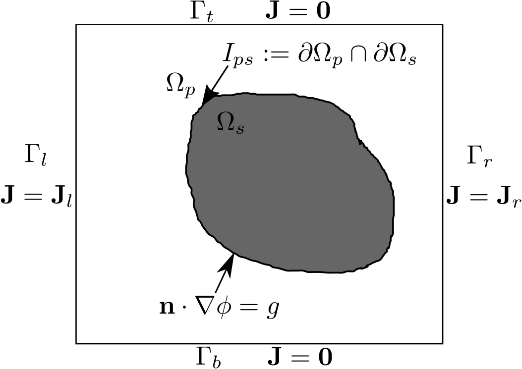
Figure 1: Flux-driven interfacial evolution taking into account specific wetting properties of an obstacle $\Omega_{s}$ by the inhomogeneous Neumann boundary condition $g=-\frac{\gamma}{C_{h}}a({\bf x})$ on $I_{ps}:=\partial\Omega_{p}\cap\partial\Omega_{s}$.

Hence, neglecting the momentum transport in thermodynamically motivated phase field formulations from (2.1) and (2.2), i.e., (2.6)₂ and (2.21)₃, respectively, leads to the following interfacial evolution problem

$$\begin{split}\boldsymbol{{\bf[A]}}\qquad\begin{cases}\quad\phi_{t}={\rm div}\left(M\nabla\left(\frac{1}{\lambda}w^{\prime}(\phi)-\lambda\Delta\phi\right)\right)\,,&\quad\text{in }\Omega_{p}\,,\\ \qquad M\nabla\left(\frac{1}{\lambda}w^{\prime}(\phi)-\lambda\Delta\phi\right)\cdot{\bf n}=J_{l}:={\bf n}\cdot{\bf J}_{l}\,,&\quad\text{on }\Gamma_{l}\,,\\ \qquad M\nabla\left(\frac{1}{\lambda}w^{\prime}(\phi)-\lambda\Delta\phi\right)\cdot{\bf n}=J_{r}:={\bf n}\cdot{\bf J}_{r}\,,&\quad\text{on }\Gamma_{r}\,,\\ \qquad{\bf n}\cdot\nabla\phi=g({\bf x})\,,&\quad\text{on }I_{ps}\,,\\ \qquad{\bf n}\cdot\nabla\phi=0\,,&\quad\text{on }\Gamma_{t}\cup\Gamma_{b}\,,\\ \qquad{\bf n}\cdot\nabla\Delta\phi=0\,,&\quad\text{on }I_{ps}\cup\Gamma_{t}\cup\Gamma_{b}\,,\\ \qquad\phi({\bf x},0)=\phi_{0}({\bf x})&\quad\text{in }\Omega_{p}\,,\end{cases}\end{split}$$ (3.32)

where $J_{l}$ and $J_{r}$ are fluxes imposed such that they drive the interface from the left to the right while neglecting momentum transport for simplicity. For the definition of the variables describing the domain $\Omega=\Omega_{p}\cup\Omega_{s}$ and its boundary $\partial\Omega=\Gamma_{l}\cup\Gamma_{r}\cup\Gamma_{t}\cup\Gamma_{b}$ as well as its interfaces $I_{ps}:=\partial\Omega_{p}\cap\partial\Omega_{s}$, we refer to Fig. 1.

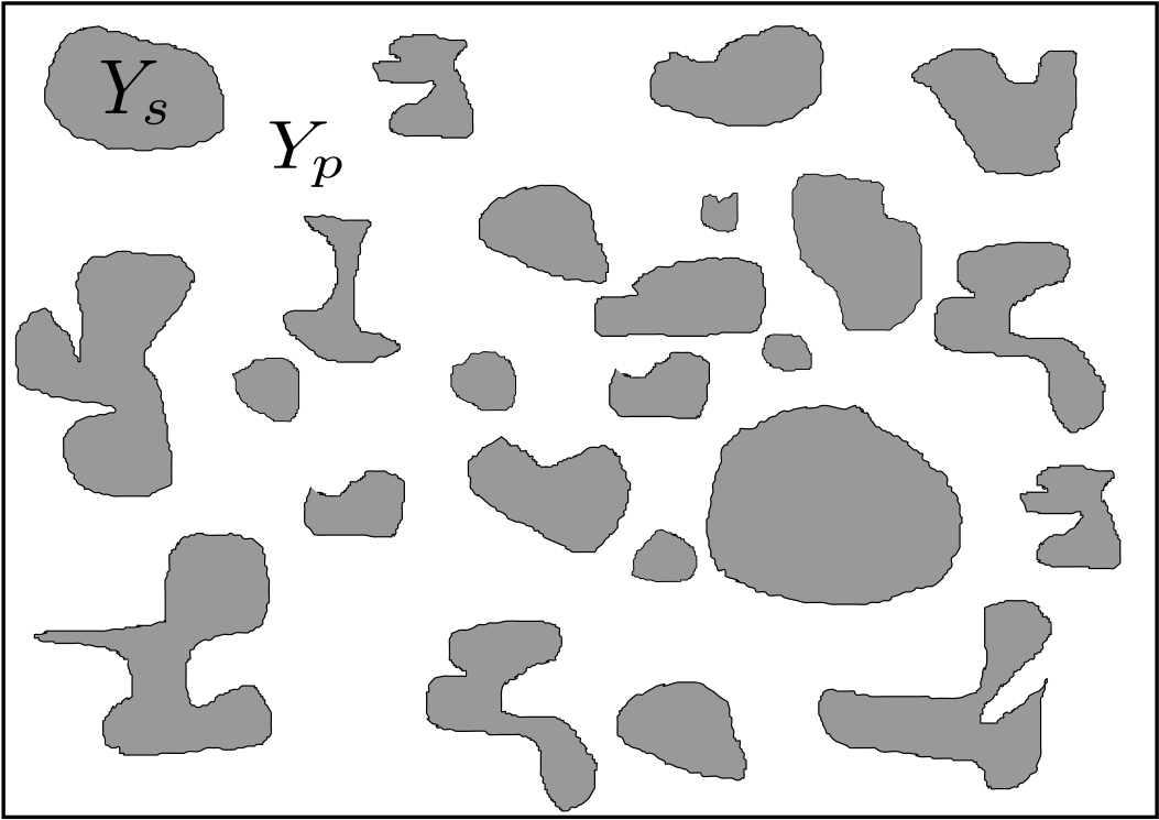
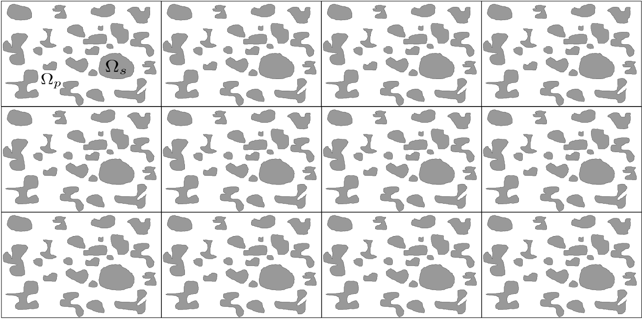
Figure 2: The upscaling of CHeSs relies on the ability to identify a characteristic reference sub-system $Y$. Left: Periodic reference cell $Y:=Y_{p}\cup Y_{s}$ with representative pore space $Y_{p}$ and characteristic solid phase $Y_{s}$. Right: Periodic porous medium $\Omega=\Omega_{p}\cup\Omega_{s}$ obtained as a covering of cells $Y$.

We would like to note that the perforated domain $\Omega_{p}$ can be defined as the subset of a porous medium $\Omega=\Omega_{p}\cup\Omega_{s}$ which is defined as the periodic covering of a reference cell $Y$, see Fig. 2, but restricted to the pore space $Y_{p}$. Herewith, a so-called heterogeneity parameter $\epsilon:=\frac{\ell}{L}$ characterising the porous medium is systematically defined as the quotient of the length of the representative porous cell $Y$ divided by the macroscopic length $L$ of the porous medium of interest. If one looks for solutions of (3.32) in a perforated domain $\Omega_{p}$ by such a periodic covering, then one can generally find $\epsilon$-dependent microscopic formulations, i.e., (3.32) rewritten by substituting $\phi$ with $\phi^{\epsilon}$, $\Omega_{p}$ with $\Omega_{p}^{\epsilon}$, and $I_{ps}$ with $I_{ps}^{\epsilon}$. For notational convenience, we do not explicitly state such an $\epsilon$-dependence of the microscopic problem here except where it is necessary for the sake of clarity.

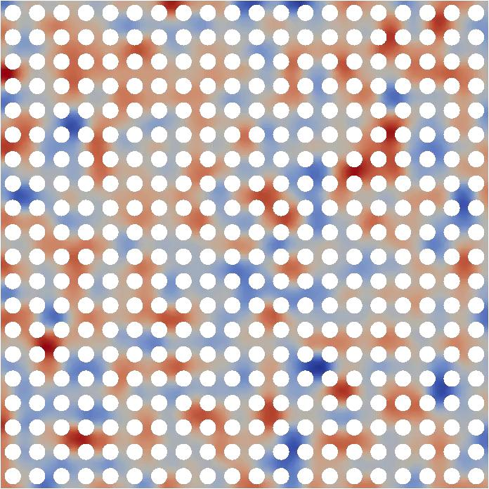
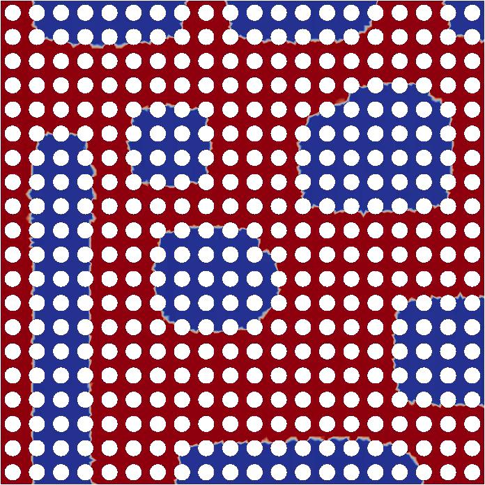
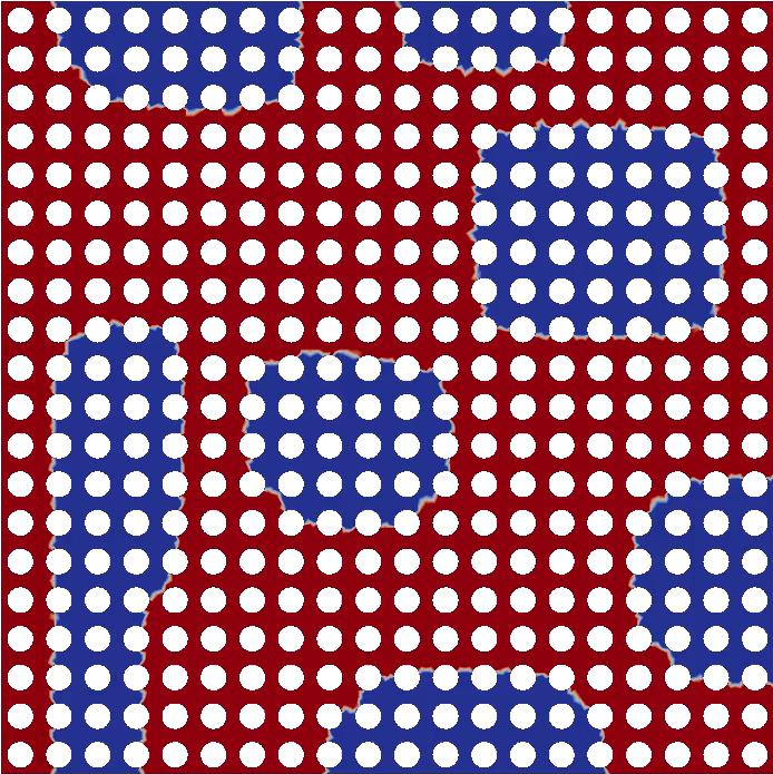
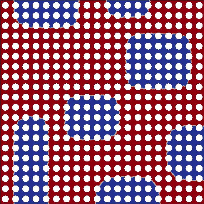
Figure 3: Time evolution [time steps 1 (top left), 5 (top right), 10 (bottom left), and 20 (bottom right)] under critical random initial conditions $\phi_{0}({\bf x})=0.5+\xi({\bf x}_{h})$ with $\xi({\bf x}_{h})\in{\cal N}(0.5,1/8)$, ${\bf x}_{h}\in{\cal T}_{h}$, where ${\cal T}_{h}$ denotes the triangulation of the connected pore space $\Omega_{p}$ obtained by removing periodically placed disks from the unit square. Hence, the computations are based on the double-well potential $w(\phi)=100\phi^{2}(1-\phi)^{2}$.

(B) Interfacial transport under quasi-static flow. We want to generalize (A) towards fluid flow. To this end, we consider a horizontal, quasi-static flow field defined in a periodic reference cell, see Fig. 2, and driven by a constant, horizontal driving force ${\bf e}_{1}$, where ${\bf e}_{1}$ is the canonical Euclidean basis. Hence, we define the fluid velocity to be the solution of the following periodic cell problem

$$\begin{split}\boldsymbol{{\bf[B1]}}\qquad\begin{cases}\quad-\mu\Delta_{\bf y}{\bf v}+\nabla_{\bf y}p={\bf e}_{1}\,,&\quad\text{in }Y_{p}\,,\\ \quad{\rm div}_{\bf y}{\bf v}=0\,,&\quad\text{in }Y_{p}\,,\\ \quad{\bf v}={\bf 0}\,,&\quad\text{on }I^{Y}_{ps}:=\partial Y_{p}\cap\partial Y_{s}\,.\end{cases}\end{split}$$ (3.33)

For large Péclet numbers scaling inversely proportional with heterogeneity, i.e., ${\rm Pe}\,={\rm Pe}\,_{0}/\epsilon$, a periodic wetting characterization $g({\bf y})=g({\bf x}/\epsilon)$ of the porous medium, and the periodic fluid velocity ${\bf v}({\bf y})={\bf v}({\bf x}/\epsilon)$, we can write the microscopic interfacial evolution problem as follows

$$\begin{split}\boldsymbol{[{\bf B2}]}\qquad\begin{cases}\quad\phi_{t}=-\frac{{\rm Pe}\,_{0}}{\epsilon}{\bf v}\cdot\nabla\phi+{\rm div}\left(\nabla\frac{1}{\lambda}w^{\prime}(\phi)-\lambda\Delta\phi\right)\,,&\quad\text{in }\Omega_{p}\,,\\ \qquad\left[-\frac{{\rm Pe}\,_{0}}{\epsilon}{\bf v}\phi+\nabla\left(\frac{1}{\lambda}w^{\prime}(\phi)-\lambda\Delta\phi\right)\right]\cdot{\bf n}=J_{l}:={\bf n}\cdot{\bf J}_{l}\,,&\quad\text{on }\Gamma_{l}\,,\\ \qquad\left[-\frac{{\rm Pe}\,_{0}}{\epsilon}{\bf v}\phi+\nabla\left(\frac{1}{\lambda}w^{\prime}(\phi)-\lambda\Delta\phi\right)\right]\cdot{\bf n}=J_{r}:={\bf n}\cdot{\bf J}_{r}\,,&\quad\text{on }\Gamma_{r}\,,\\ \qquad{\bf n}\cdot\nabla\phi=g({\bf x}/\epsilon)\,,&\quad\text{on }I_{ps}\,,\\ \qquad{\bf n}\cdot\nabla\phi=0\,,&\quad\text{on }\Gamma_{t}\cup\Gamma_{b}\,,\\ \qquad{\bf n}\cdot\nabla\Delta\phi=0\,,&\quad\text{on }I_{ps}\cup\Gamma_{t}\cup\Gamma_{b}\,,\\ \qquad\phi({\bf x},0)=\phi_{0}({\bf x})\,,&\quad\text{in }\Omega_{p}\,,\end{cases}\end{split}$$ (3.34)

where we have set the mobility to $M=1$ for simplicity.

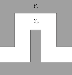
Figure 4: Reference sub-substem $Y:=Y_{p}\cup Y_{s}$ defining the representative microscale.

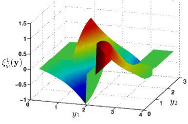
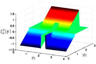
Figure 5: Top line: Heterogeneous system correctors $\xi^{1}$ and $\xi^{2}$ solving the cell problem (reference sub-system) (3.37) and the perturbed straight channel Fig. 4. Bottom line: Components $v^{1}$ and $v^{2}$ solving (3.33) in the reference cell Fig. 4/

3.1 Effective macroscopic interfacial evolution and error quantification

The microscopic formulations (3.32) and (3.33)-(3.34) lead to computationally high-dimensional problems since the mesh size needs to be chosen much smaller than the heterogeneity $\epsilon$. Also defining the pore and solid space together with the associated interfaces, which are generally obtained with the help of imaging tools, is rather challenging for such complex geometries such as porous media. Moreover, the subsequent mesh generation is also more demanding due to the complex geometries requiring a large number of degrees of freedom for a reliable resolution.

As a consequence, one can accelerate the computation of practical problems by identifying the characteristic pore geometry for a smaller representative volume element, e.g., by a reference cell $Y$ as depicted in Fig. 2, which contains all the relevant information about geometry. For such a reference cell, the mesh generation and associated domain definitions can be done faster in an offline calculation to extract relevant geometric information. A systematic method, that allows for such a splitting into an offline pre-processing and an online computation of an effective interfacial evolution problem, are asymptotic upscaling/homogenization methods. Here, we state two recent upscaling results which represent homogenized formulations of the microscopic descriptions $\boldsymbol{[{\bf A}]}$ and $\boldsymbol{[{\bf B1}]}$–$\boldsymbol{[{\bf B2}]}$ stated in (3.32) and (3.33)–(3.34), respectively.

(A) Upscaled formulation for the interfacial transport problem (3.32). The systematic upscaling based on asymptotic two-scale expansions of the form $\phi^{\epsilon}=\phi^{0}({\bf x},{\bf x}/\epsilon,t)+\epsilon\phi^{1}({\bf x},{\bf x}/\epsilon,t)+\epsilon^{2}\phi^{2}({\bf x},{\bf x}/\epsilon,t)+\dots\,,$ have been applied in [36, 35] to derive the following effective macroscopic formulation of (3.32), i.e.,

$$\begin{split}\boldsymbol{[{\bf A}_{\rm eff}]}\qquad\begin{cases}\quad p\phi_{t}={\rm div}\left(M\hat{\rm D}\nabla\left(\frac{1}{\lambda}w^{\prime}(\phi)-{\rm div}\left(\frac{\lambda}{p}\hat{\rm D}\nabla\phi\right)\right)\right)\,,&\quad\text{in }\Omega\,,\\ \qquad M\hat{\rm D}\nabla\left(\frac{1}{\lambda}w^{\prime}(\phi)-{\rm div}\left(\frac{\lambda}{p}\hat{\rm D}\nabla\phi\right)\right)\cdot{\bf n}=J_{l}:={\bf n}\cdot{\bf J}_{l}\,,&\quad\text{on }\Gamma_{l}\,,\\ \qquad M\hat{\rm D}\nabla\left(\frac{1}{\lambda}w^{\prime}(\phi)-{\rm div}\left(\frac{\lambda}{p}\hat{\rm D}\nabla\phi\right)\right)\cdot{\bf n}=J_{r}:={\bf n}\cdot{\bf J}_{r}\,,&\quad\text{on }\Gamma_{r}\,,\\ \qquad{\bf n}\cdot\hat{\rm D}\nabla\phi=0\,,&\quad\text{on }\Gamma_{t}\cup\Gamma_{b}\,,\\ \qquad{\bf n}\cdot\hat{\rm D}\nabla{\rm div}\left(\frac{1}{p}\hat{\rm D}\nabla\phi\right)=0\,,&\quad\text{on }I_{ps}\cup\Gamma_{t}\cup\Gamma_{b}\,,\\ \qquad\phi({\bf x},0)=\phi_{0}({\bf x})&\quad\text{in }\Omega_{p}\,,\end{cases}\end{split}$$ (3.35)

where $p:=\frac{\left|Y_{p}\right|}{\left|Y\right|}$ is the porosity and the porous media correction tensor $\hat{\rm D}=\left\{d_{ij}\right\}_{1\leq i,j\leq d}$ is defined by

$$\begin{split}d_{ij}:=\frac{1}{|Y|}\sum_{k=1}^{d}\int_{Y_{p}}\left(\delta_{ij}-\delta_{ik}\frac{\partial\xi^{j}}{\partial y_{k}}\right)\,d{\bf y}\,.\end{split}$$ (3.36)

Finally, the porous media corrector $\xi^{k}$, $1\leq k\leq d$, solves the following reference cell problem

$$\begin{split}\begin{cases}\quad-\sum_{i,j=1}^{d}\frac{\partial}{\partial y_{i}}\left(\delta_{ij}\frac{\partial({\bf y}_{k}-\xi^{k})}{\partial y_{j}}\right)=0\,,\\ \quad\sum_{i,j=1}^{d}n_{i}\left(\delta_{ij}\frac{\partial({\bf y}_{k}-\xi^{k})}{\partial y_{j}}\right)=0\,,&\qquad\text{on }\partial Y_{p}\,,\\ \quad\xi^{k}({\bf y})\text{ is $Y_{p}$-periodic and $\int_{Y}\xi^{k}\,d{\bf y}=0$\,,}\end{cases}\end{split}$$ (3.37)

which is of the same form as the cell problems obtained in the homogenization of elliptic equations such as the Laplace and Poisson equations, e.g. [2, 10].

This novel effective macroscopic phase field formulation has been recently rigorously justified by a first error quantification in [34]. If we adopt the notation generally applied in homogenization theory, then one explicitly states the $\epsilon$-dependence of solutions (i.e., $\phi^{\epsilon}$) of the microscopic formulation $\boldsymbol{[{\bf A}]}$ and since the upscaling consists in passing to the limit $\epsilon\to 0$, one writes $\phi^{0}$ for the solution of the effective macroscopic problem $\boldsymbol{[{\bf A}_{\rm eff}]}$. Hence, if the free energy density $f_{r}$ is polynomial, then the error variable ${\rm E}^{\phi}_{\epsilon}:=\phi^{\epsilon}-(\phi_{0}+\epsilon\phi_{1})\,,$ where $\phi_{1}:=-\sum_{k=1}^{d}\xi^{k}_{\phi}({\bf y})\frac{\partial\phi_{0}}{\partial x_{k}}({\bf x},t)$, satisfies for $0\leq t\leq T$ and $0<T<\infty$ the following estimate

$$\begin{split}\left\|E_{\epsilon}^{\phi}(\cdot,t)\right\|_{H^{1}(\Omega^{\epsilon})}:=\left(\int_{\Omega^{\epsilon}}\left(\left|E_{\epsilon}^{\phi}({\bf x},t)\right|^{2}+\left|\nabla E_{\epsilon}^{\phi}({\bf x},t)\right|^{2}\right)\,d{\bf x}\right)^{1/2}&\leq\epsilon^{1/4}C(T,\Omega,m,\kappa,\lambda)\,,\end{split}$$ (3.38)

where $C(T,\Omega,m,\kappa,\lambda)$ is a constant independent of $\epsilon$.

We note that the convergence rate ${\cal O}(\epsilon^{1/4})$ arises due to the classical argument of relying on a smooth truncation in a neighbourhood of the boundary. A numerical validation of the error bound (3.38) and recent developments of novel estimation techniques such as [30, 38], indicate a linear convergence, i.e., ${\cal O}(\epsilon)$. Hence, we hope that this first rigorous result for fourth order problems motivates the future refinement towards a sharp error quantification.

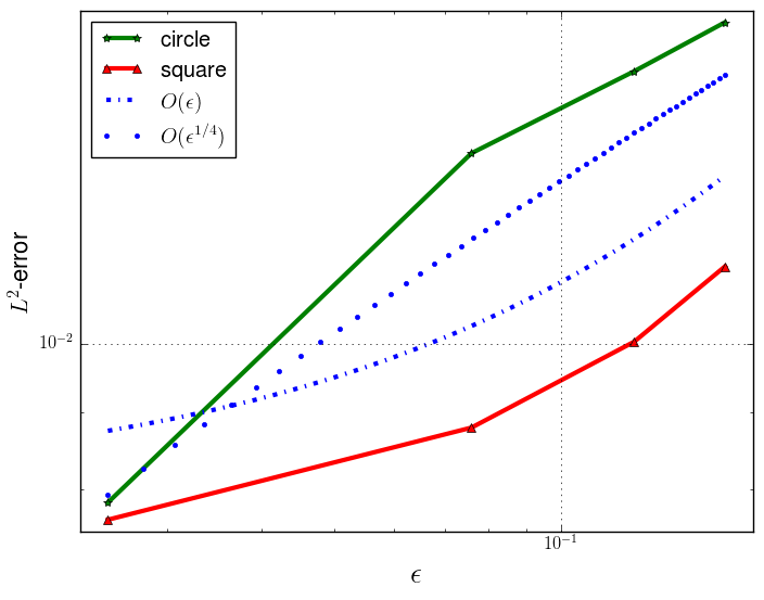
Figure 6: The converge for $\epsilon\in\left\{0.025,0.076,0.125,0.165\right\}$ (right) has been computed for perforated meshes by removing discs (left) and squares (middle).

(B) Upscaled transport formulation for the quasi-static flow problem (3.33)–(3.34). Next to systematically and reliably describing interfacial dynamics in strongly heterogeneous systems, we also want to account for so-called diffusion-dispersion effects of the interface. This latter phenomenon is well-known for Brownian particles where it has been motivated by the so-called Taylor-Aris dispersion in [3, 39]. Here, we state the recent upscaling result derived in [37] for the microscopic problem (3.33)–(3.34), i.e., $\boldsymbol{[{\bf B1}]}$–$\boldsymbol{[{\bf B2}]}$,

$$\begin{split}\begin{cases}\quad p\phi_{t}={\rm div}\left(\left(\hat{\rm C}+\frac{1}{\lambda}\hat{\rm D}w^{\prime\prime}(\phi)\right)\nabla\phi\right)-{\rm div}\left(\hat{\rm D}\nabla\left(\frac{\lambda}{p}{\rm div}\left(\hat{\rm D}\nabla\phi\right)-\overline{g}\right)\right)\,,&\quad\text{in }\Omega\,,\\ \qquad\left(\left(\hat{\rm C}+\frac{1}{\lambda}\hat{\rm D}w^{\prime\prime}(\phi)\right)\nabla\phi+\nabla\left(\frac{\lambda}{p}{\rm div}\left(\hat{\rm D}\nabla\phi\right)-\overline{g}\right)\right)\cdot{\bf n}=J_{l}:={\bf n}\cdot{\bf J}_{l}\,,&\quad\text{on }\Gamma_{l}\,,\\ \qquad\left(\left(\hat{\rm C}+\frac{1}{\lambda}\hat{\rm D}w^{\prime\prime}(\phi)\right)\nabla\phi+\nabla\left(\frac{\lambda}{p}{\rm div}\left(\hat{\rm D}\nabla\phi\right)-\overline{g}\right)\right)\cdot{\bf n}=J_{r}:={\bf n}\cdot{\bf J}_{r}\,,&\quad\text{on }\Gamma_{r}\,,\\ \qquad{\bf n}\cdot\hat{\rm D}\nabla\phi=0\,,&\quad\text{on }\Gamma_{t}\cup\Gamma_{b}\,,\\ \qquad{\bf n}\cdot\hat{\rm D}\nabla\left(\frac{\lambda}{p}{\rm div}\left(\hat{\rm D}\nabla\phi\right)-\overline{g}\right)=0\,,&\quad\text{on }I_{ps}\cup\Gamma_{t}\cup\Gamma_{b}\,,\\ \qquad\phi({\bf x},0)=\phi_{0}({\bf x})&\quad\text{in }\Omega_{p}\,,\end{cases}\end{split}$$ (3.39)

where the porous media correction tensor $\hat{\rm D}$ is defined by (3.36) and (3.37) as in the case of ${\bf v}={\bf 0}$. At the same time, we have a new tensor $\hat{\rm C}:=\left\{c_{ij}\right\}_{1\leq i,j\leq d}$ contributing to the so-called diffusion-dispersion effects by

$$\begin{split}c_{ik}:=\frac{{\rm Pe}\,_{0}}{\left|Y\right|}\int_{Y^{1}}\left(v^{i}-u^{i}\right)\delta_{ik}\xi^{k}_{\phi}\,d{\bf y}\,,\end{split}$$ (3.40)

with $\xi^{k}_{\phi}$ being the solution of the cell problem (3.37), $u^{i}:=\frac{Pe_{0}}{\left|Y\right|}\int_{Y_{p}}v^{i}({\bf y})\,d{\bf y}$ for $v^{i}$ given by (3.33), and the effective wetting term is given by $\overline{g}:=-\frac{\gamma}{C_{h}}\frac{1}{\left|Y\right|}\int_{\partial Y^{1}}a({\bf x},{\bf y})\,d{\bf y}\,,$ for wetting characteristics $a$ varying on the macro- and the microscale.

Finally, we emphasize that the advantage of the novel upscaled formulation (3.39) is that it allows for a computational decoupling into an offline computation resolving the microscopic features of CHeSs and an online computation to solve the low-dimensional, effective macroscopic phase field equation accounting for diffusion-dispersion relations. We believe that this novel approach will be useful in many applications since it allows to take systematic thermodynamic free energies into account and hence provides a promising framework for investigating complex reactive multiphase flows.

3.2 Universal coarsening rates: ${\cal O}(t^{1/3})$-behaviour recovered in heterogeneous media

The first systematic report on the radial dependence of the coarsening/ripening process seems to go back to Ostwald in 1900. Since this “Ostwald ripening” happens in almost all phase transition processes and governs the morphology of microstructure, Ostwald’s discovery of this competitive growth phenomenon plays a crucial role in materials science and related applications. An important property of the morphology is its self-similarity which one can observe after sufficiently long coarsening times. The physical explanation for the Ostwald ripening is that the system tries to minimize its energy by reducing the system’s interfacial area. Moreover, coarsening relies on the fact that a single large particle has much lower interfacial area than many small particles. We note that this ripening/coarsening appears in different characteristic length scales such as distance between particles, particle radius, or the inverse of the interfacial area per volume, i.e., $L(t)=\left|D\right|/E_{\rm mix}$, where $\frac{1}{\left|D\right|}E_{\rm mix}$ is the volume-averaged interfacial area which relies on the Cahn-Hilliard free energy density $f_{\rm mix}$, see (2.28). Here, we will focus on this latter length $L$.

About 60 years later since Ostwald’s discovery of this growth phenomenon, Lifshitz and Slyozov [22] and Wagner [43] proposed a mean field equation whose solution gives the number of droplets of a particular radius $r$ at time $t$. The following coarsening rate

$$\begin{split}L(t)\leq Ct^{1/3}\,,\end{split}$$ (3.41)

has been validated experimentally and computationally in [45]. So far, a rigorous proof for (3.41) has only been obtained for a time-averaged version in [19], i.e.,

$$\begin{split}\frac{1}{T}\int_{0}^{T}E_{\rm mix}^{2}\,dt\geq\frac{C}{T}\int_{0}^{T}\left(t^{-1/3}\right)^{2}\,dt\,.\end{split}$$ (3.42)

In [42], the authors have recently studied the influence of heterogeneities such as periodic porous media on the coarsening rate. Here, we extended this validation towards non-periodic porous media with porosity gradients, see Fig. 7. We observe that the well-known coarsening rate (3.41) for homogeneous media also holds in the context of porous media under neutral wetting conditions, i.e., a contact angle of $90^{\circ}$. Hence, this indicates that the exponent $1/3$ in (3.41) represents a universal coarsening rate.

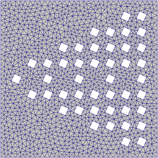
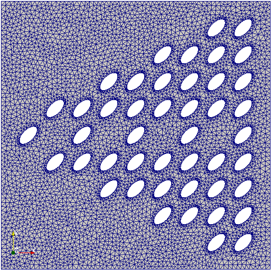
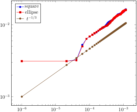
Figure 7: Left and Middle: Different geometries and porosity gradients. Right: Coarsening rate seems to be universal, i.e., independent of pore geometries and porosity gradients.

4 Application of $\boldsymbol{[{\bf A}_{\rm eff}]}$: upscaled composite cathodes

Batteries represent a delicate CHeSs due to mass and charge transport through different phases such as an active anode and a composite cathode which are separated by a polymer electrolyte. Moreover, the performance of batteries crucially depends on interfacial reactions, generally described by Butler-Volmer reactions. A schematic design of a lithium-ion battery is depicted in Fig. 8 (left).

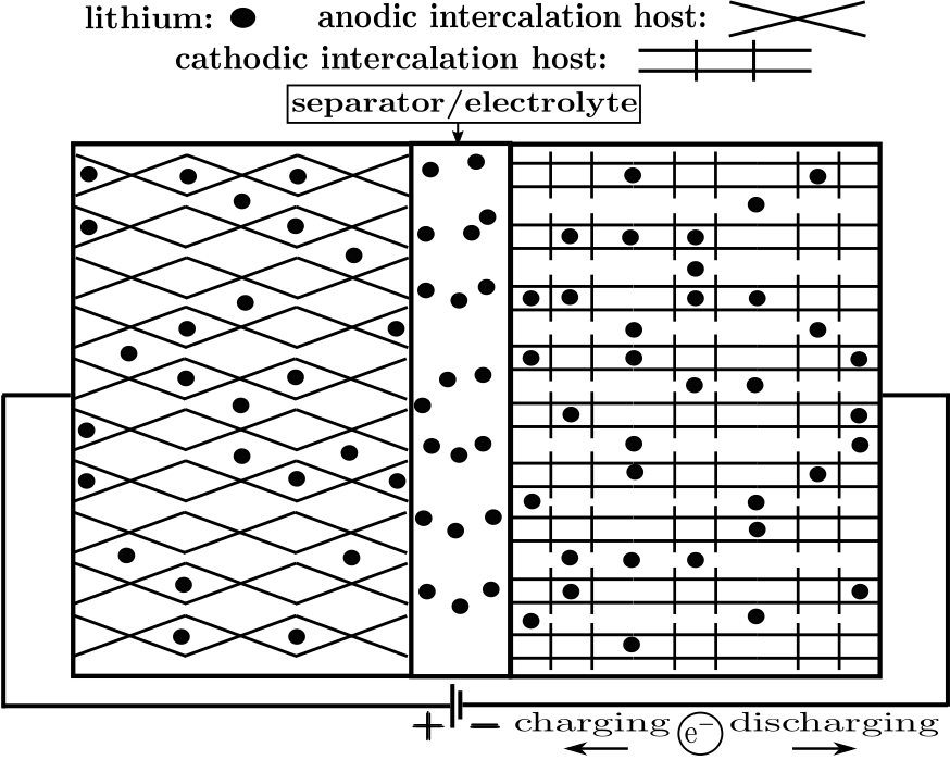
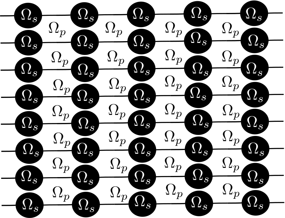
Figure 8: Left: lithium-ion battery with two active electrodes, i.e., anode and cathode separated by a polymer electrolyte. The left- and right-hand vertical boundaries are current collectors. Right: A three-phase composite cathode $\Omega:=\Omega_{p}\cup\Omega_{s}\cup\Omega_{b}$ showing two-phase fiber composites $\Omega_{p}\cup\Omega_{b}$ separated vertically by the polymer electrolyte $\Omega_{p}$. The binder $\Omega_{b}$ connecting the solid intercalation hosts $\Omega_{s}$ enables electron conduction towards the current collector.

For simplicity, we restrict ourselves to the composite cathode which consists of solid intercalation particles $\Omega_{s}$, a polymer electrolyte phase $\Omega_{p}$, and an electron conducting binder $\Omega_{b}$ allowing for electron conduction between the solid phase $\Omega_{s}$. An example of a composite cathode is given in Fig. 8 (right), which represents horizontal fibers separated by a polymer electrolyte. We note that an effective model formulation for composite cathodes has been proposed in [11] with the help of a so-called shrinking core description relying on radial and classical diffusion. In this section, we present a recently derived generalization towards an effective macroscopic formulation accounting for interstitial diffusion in heterogeneous domains.

Motivated by the experimental fact that crystalline intercalation hosts of composite cathodes can phase separate, and by the increased interest in describing lithium intercalation by a phase field equation as initiated in [15] and further developed in [5, 6, 8], an effective composite cathode formulation based on phase field driven intercalation and dilute electrolytes has been systematically derived recently in [33]. Hence, the incompressible momentum ${\bf V}$, the densities $C^{+}$ and $C^{-}$ of positively and negatively charged ions, respectively, the electrostatic potentials $\Psi_{s}$ and $\Psi_{p}$ for the solid and electrolyte phase, respectively, as well as the density of intercalated lithium $C^{s}$ are described by the following novel upscaled composite cathode system,

$$\begin{split}\begin{cases}\quad{\bf V}({\bf x},t)=-\frac{\hat{\kappa}}{\mu}\left({\bf f}^{0}-\nabla P\right)&\quad\text{in }\Omega\,,\\ \qquad{\rm div}\,{\bf V}=0\,,&\quad\text{in }\Omega\,,\\ \quad p\partial_{t}C^{+}+{\rm Pe}\,{\bf V}\cdot\nabla C^{+}={\rm div}\left(\hat{\mathbb{D}}\nabla C^{+}+z_{+}C^{+}\hat{\mathbb{M}}\nabla\Psi_{p}\right)-\overline{\beta}_{+}R(C^{+},C^{s},\eta^{0},U^{0})&\quad\text{in }\Omega\,,\\ \quad p\partial_{t}C^{-}+{\rm Pe}\,{\bf V}\cdot\nabla C^{-}={\rm div}\left(\hat{\mathbb{D}}\nabla C^{-}-z_{-}C^{-}\hat{\mathbb{M}}\nabla\Psi_{p}\right)&\quad\text{in }\Omega\,,\\ \quad-{\rm div}\left(\hat{\varepsilon}\nabla\Psi_{p}\right)=p\left(z_{+}C^{+}+z_{-}C^{-}\right)&\quad\text{in }\Omega\,,\\ \quad-{\rm div}\left(\hat{\Sigma}\nabla\Psi_{s}\right)=\overline{\beta}_{\psi}R(C^{+},C^{s},\eta^{0},U^{0})&\quad\text{in }\Omega\,,\\ \quad q\partial_{t}C^{s}={\rm div}\left(\hat{\mathbb{M}}_{s}\left(\nabla f_{r}^{\prime}(C^{s})+\frac{\lambda}{q}{\rm div}\left(\hat{\mathbb{M}}_{s}\nabla C^{s}\right)\right)\right)+\overline{\beta}_{s}R(C^{+},C^{s},\eta^{0},U^{0})&\quad\text{in }\Omega\,,\end{cases}\end{split}$$ (4.43)

where $p=\frac{|Y_{p}|}{|Y|}$ is the porosity (see Fig. 2), $q=1-p$, ${\bf f}^{0}=-\eta\left(C^{+}-C^{-}\right)\hat{\mathbb{M}}\nabla\Psi_{p}$ an effective Coulomb force, and the material’s correction tensors $\hat{\kappa}=\left\{\overline{\kappa}_{ij}\right\}_{i,j=1}^{d}$, $\hat{\mathbb{M}}=\left\{\overline{m}_{ij}\right\}_{i,j=1}^{d}$, $\hat{\mathbb{D}}=\left\{\overline{d}_{ij}\right\}_{i,j=1}^{d}$, $\hat{\varepsilon}=\left\{\overline{\varepsilon}_{ij}\right\}_{i,j=1}^{d}$, $\hat{\Sigma}=\left\{\overline{\sigma}_{ij}\right\}_{i,j=1}^{d}$, and $\hat{\mathbb{M}}_{s}=\left\{\overline{m}^{s}_{ij}\right\}_{i,j=1}^{d}$ are defined by standard cell problems arising in the homogenization theory (see (3.37) and (3.36) for instance) and therefore we refer the interested reader to [33]. Finally, the interfacial Butler-Volmer reactions

$$\begin{split}R=i_{ps}\left[\frac{C^{s}}{c_{sm}}\exp\left(\alpha_{sm}\frac{\alpha_{a}F}{RT}(\eta^{0}-U^{0})\right)-\frac{(c_{\rm sm}-C^{s})}{c_{sm}}\exp\left(-\alpha_{sm}\frac{\alpha_{c}F}{RT}(\eta^{0}-U^{0})\right)\right]\,,\end{split}$$ (4.44)

appear in the upscaled system (4.43) as bulk equations and show the important coupling parameters $\overline{\beta}_{+}=\frac{i_{0}L|\Lambda|}{eD}$, $\overline{\beta}_{\psi}=\frac{F}{RT}\frac{i_{ps}L|\Lambda|}{\sigma_{ref}}$, $\overline{\beta}_{s}=\frac{i_{0}L|\Lambda|}{eM_{s}}$, for $\sigma_{ref}=\frac{\varepsilon_{p}D}{\lambda_{D}^{2}}\,.$ Moreover, $\eta^{0}=\Psi_{s}-\Psi_{p}$ denotes the overpotential and $U^{0}$ represents the open circuit potential. Finally, the variable $i_{ps}=Fk_{\rm fb}(c_{\rm pm}^{\epsilon_{p}}-c^{\epsilon_{p}})^{\alpha_{c}}(c^{\epsilon_{p}})^{\alpha_{a}}$ is the so-called exchange current density and $c_{sm}^{\epsilon_{p}}={\rm exp}\left(\alpha_{sm}\right)\,.$

The novel system (4.43) shares with the crucial modelling initiated in [11] the fact that in the effective macroscopic formulation, the different phases are superimposed or homogenized (referring to the underlying upscaling strategy). The main novelty and contribution of (4.43) is the appearance of the effective phase field equation (4.43)₇ generalizing the radial diffusion (shrinking core) formulation proposed in [11] towards a thermodynamic formulation taking phase separation during the lithium intercalation into account.

5 Conclusions

We have presented recent developments to describe interfacial evolution of binary mixtures founded on the non-equilibrium thermodynamic structure provided by the reversible-irreversible couplings, called GENERIC. And we highlighted the increasing interest in establishing a non-equilibrium variational principle by generalising the least action principle for reversible systems to acccount for the right irreversible contributions via a maximum dissipation principle in Section 2.

A major part of this article has then been devoted to demonstrate that reliable upscaling of phase field equations provides a new and thermodynamic consistent approach to describe multiphase flow in porous media. In fact, the novel formulations (3.35) (without flow) and (3.39) (with flow) take the underlying, thermodynamic free energy of fluid mixtures into account in difference to the classical multiphase extension (3.30) of Darcy’s law. It is noteworthy that Darcy’s law represents from a thermodynamic point of view a reduced momentum balance equation. Moreover, under quasi-static fluid flow defined on a reference cell in local thermodynamic equilibrium, our upscaled/effective multiphase flow formulation includes the so-called diffusion-dispersion relations which have been intensively studied in the context of Brownian motion/Fick’s diffusion, e.g. [3, 39]. In fact, the effective macroscopic phase field formulation (3.35) has been analytically and computationally validated by error estimates, i.e., inequality (3.38) and Fig. 6 (right), respectively. Additionally, we investigated the effect of heterogeneities, e.g. perforated domains with porosity gradients as depicted in Fig. 7, on the coarsening rate and, interestingly, we observe that the coarsening rate ${\cal O}(t^{1/3})$, well-known for homogeneous domains, also holds in porous media and hence seems to represent a universal property.

Of course the Cahn-Hilliard phase field equation [9] has a long history going back to 1958. Since then, there is a continuously increasing interest in applying the mean field formulation in a wide spectrum of fields including physics, material science, biology, and fluid dynamics to mention but a few. We believe that the novel multiphase flow/interfacial evolution equations we outlined, show promise for a wide range of scientific, engineering, and industrial applications. And we hope that they can motivate further studies on the use of non-equilibrium thermodynamic framework we described for problems where heterogeneities play a crucial role. A rather novel direction is battery science as initiated in [15], where the phase field model has been motivated as a reliable description for interstitial diffusion. This has found increasing interest in computational material science and electrochemistry and hence motivated us to present here the extension of this description to systematically account for highly heterogeneous electrodes such as composite cathodes, see Fig. 8 for instance.

References

- [1] H. Abels, H. Garcke, and G. Grün. Thermodynamically consistent, frame indifferent diffuse interface models for incompressible two-phase flows with different densities. Math. Mod. Meth. Appl. S., 22(03):1150013, March 2012.
- [2] G. Allaire. Homogenization and two-scale convergence. SIAM J. Math. Anal., 23(6):1482–1518, 1992.
- [3] R. Aris. On the Dispersion of a Solute in a Fluid Flowing through a Tube. Proc. R. Soc. A, 235(1200):67–77, 1956.
- [4] S. Arnrich, A. Mielke, M.A. Peletier, G. Savaré, and M. Veneroni. Passing to the limit in a Wasserstein gradient flow: from diffusion to reaction. Calculus of Variations and Partial Differential Equations, 44(3-4):419–454, August 2012.
- [5] P. Bai, D.A. Cogswell, and M.Z. Bazant. Suppression of phase separation in lifepo4 nanoparticles during battery discharge. Nano Letters, 11(11):4890–4896, 2011. PMID: 21985573.
- [6] M.Z. Bazant. Theory of chemical kinetics and charge transfer based on nonequilibrium thermodynamics. Accounts of Chemical Research, 46(5):1144–1160, 2013. PMID: 23520980.
- [7] S. Bosia, M. Conti, and M. Grasselli. On the cahn-hilliard-brinkman system. arXiv:1402.6195, 2014.
- [8] D. Burch, G. Singh, G. Ceder, and M.Z. Bazant. Phase-transformation wave dynamics in LiFePO4. Solid State Phenomena, 139:95–100, 2008.
- [9] J.W. Cahn and J.E. Hilliard. Free Energy of a Nonuniform System. I. Interfacial Free Energy. J. Chem. Phys., 28(2):258, 1958.
- [10] G. A. Chechkin, A. L. Piatnitski, and A. S. Shamaev. Homogenization: Methods and Applications. American Mathematical Society, 2007.
- [11] M. Doyle, T.F. Fuller, and J. Newman. Modeling of Galvanostatic Charge and Discharge of the Lithium/Polymer/Insertion Cell. J. Electrochem. Soc., 140(6):1526, 1993.
- [12] P. Ehrenfest. Phasenumwandlungen im ueblichen und erweiterten Sinn, classifiziert nach den entsprechenden des thermodynamischen Potentials. zu den Mitteilungen aus dem KAMERLINGH ONNES-Institut, Leiden, Supplement No. 75b, 1933.
- [13] M. Grmela and H. C. Öttinger. Dynamics and thermodynamics of complex fluids.i. development of a general formalism. Phys. Rev. E, 56:6620–6632, Dec 1997.
- [14] K. Hackl and F.D. Fischer. On the relation between the principle of maximum dissipation and inelastic evolution given by dissipation potentials. Proc. R. Soc. A, 464(2089):117–132, January 2008.
- [15] B.C. Han, A. Van der Ven, D. Morgan, and G. Ceder. Electrochemical modeling of intercalation processes with phase field models. Electrochimica Acta, 49(26):4691–4699, October 2004.
- [16] Y. Hyon, D.Y. Kwak, and C. Liu. Energetic variational approach in complex fluids: Maximum dissipation principle. Discrete Cont. Dyn. S., 26(4):1291–1304, December 2010.
- [17] A. Jelic. Bridging scales in complex fluids out of equilibrium. PhD thesis, ETH Zurich, 2009.
- [18] R. Jordan, D. Kinderlehrer, and F. Otto. The Variational Formulation of the Fokker-Planck Equation. SIAM J. Math. Anal., 29(1):1, 1998.
- [19] V.R. Kohn and F. Otto. Upper bounds on coarsening rates. Communications in Mathematical Physics, 229(3):375–395, 2002.
- [20] J.W. Leech. Classical Mechanics. Methuen & CO. LTD and Science Paperbacks, 1965.
- [21] M.C. Leverett. Capillary behavior in porous solids. Society of Petroleum Engineers, 1941.
- [22] I.M. Lifshitz and V.V. Slyozo. The kinetics of precipitation from supersaturated solid solutions. J. Phys. Chem. Solids, 19:35–50, 1961.
- [23] C. Liu and J. Shen. A phase field model for the mixture of two incompressible fluids and its approximation by a Fourier-spectral method. Physica D: Nonlinear Phenomena, 179(3-4):211–228, May 2003.
- [24] A. Mielke. A gradient structure for reaction–diffusion systems and for energy-drift-diffusion systems. Nonlinearity, 24(4):1329–1346, April 2011.
- [25] I. Müller and T. Ruggeri. Extended thermodynamics. Springer New York, 1993.
- [26] M. Muskat and M.W. Meres. The flow of heterogeneous fluids through porous media. Physics, 7(9):346–363, 1936.
- [27] A Novick-Cohen. The {C}ahn-{H}illiard equation, volume 4 of Handb. Differ. Equ., pages 201–228. Elsevier/North-Holland, Amsterdam, 2008.
- [28] H.C. Öttinger. Beyond Equilibrium Thermodynamics. Wiley, 2004.
- [29] H.C. Öttinger and M. Grmela. Dynamics and thermodynamics of complex fluids. ii. illustrations of a general formalism. Phys. Rev. E, 56:6633–6655, Dec 1997.
- [30] S.E. Pastukhova. The dirichlet problem for elliptic equations with multiscale coefficients. operator estimates for homogenization. Journal of Mathematical Sciences, 193(2):283–300, 2013.
- [31] M. Pradas, N. Savva, J. B. Benziger, I. G. Kevrekidis, and S. Kalliadasis. Dynamics of fattening and thinning 2d sessile droplets. Langmuir, 32(19):4736–4745, 2016. PMID: 27077328.
- [32] N. Savva, S. Kalliadasis, and G.A. Pavliotis. Two-dimensional droplet spreading over random topographical substrates. Phys. Rev. Lett., 104:84501, 2010.
- [33] M. Schmuck. Upscaling of solid-electrolyte composite intercalation cathodes for energy storage systems. Appl. Math. Res. Express, pages 1–29, 2017.
- [34] M. Schmuck and S. Kalliadasis. Rate of convergence of general phase field equations in strongly heterogeneous media toward their homogenized limit. SIAM Journal on Applied Mathematics, 77(4):1471–1492, 2017.
- [35] M. Schmuck, G.A. Pavliotis, and S. Kalliadasis. Effective macroscopic interfacial transport equations in strongly heterogeneous environments for general homogeneous free energies. Appl. Math. Lett., 35:12–17, 2014.
- [36] M. Schmuck, M. Pradas, G. A. Pavliotis, and S. Kalliadasis. Upscaled phase-field models for interfacial dynamics in strongly heterogeneous domains. Proc. R. Soc. A, 468(2147):3705–3724, jun 2012.
- [37] M. Schmuck, M. Pradas, G.A. Pavliotis, and S. Kalliadasis. Derivation of effective macroscopic Stokes–Cahn–Hilliard equations for periodic immiscible flows in porous media. Nonlinearity, 26(12):3259, 2013.
- [38] T.A. Suslina. Operator error estimates in for homogenization of an elliptic dirichlet problem. Funct. Anal. Appl., 46(3):234–238, 2012.
- [39] G. Taylor. Dispersion of Soluble Matter in Solvent Flowing Slowly through a Tube. Proc. R. Soc. A, 219(1137):186–203, August 1953.
- [40] J.D. Van Der Waals. The thermodynamic theory of capillarity under the hypothesis of a continuous variation of density. Verhandel Konink. Akad. Weten. Amsterdam (Sec. 1), 1:1–56. Translation by J.S. Rowlingson, 1979, J. Stat. Phys. 20,197–233., 1892.
- [41] R. Vellingiri, N. Savva, and S. Kalliadasis. Droplet spreading on chemically heterogeneous substrates. Phys. Rev. E, 84:036305, 2011.
- [42] A. Ververis and M. Schmuck. Computational investigation of porous media phase field formulations: Microscopic, effective macroscopic, and langevin equations. Journal of Computational Physics, 344(Supplement C):485 – 498, 2017.
- [43] C. Wagner. Theorie der alterung von niederschlägen durch umlösen. Z. Elektrochmie, 65:581–594, 1961.
- [44] C. Wylock, M. Pradas, B. Haut, P. Colinet, and S. Kalliadasis. Disorder-induced hysteresis and nonlocality of contact line motion in chemically heterogeneous microchannels. Physics of Fluids, 24(3):32108, 2012.
- [45] J. Zhu, L.-Q. Chen, J. Shen, and V. Tikare. Coarsening kinetics from a variable-mobility cahn-hilliard equation: Application of a semi-implicit fourier spectral method. Phys. Rev. E, 60:3564–3572, Oct 1999.