Infrared modified gravity with propagating torsion:
instability of torsionfull de Sitter-like solutions

Abstract

We continue the exploration of the consistency of a modified-gravity theory that generalizes General Relativity by including a dynamical torsion in addition to the dynamical metric. The six-parameter theory we consider was found to be consistent around arbitrary torsionless Einstein backgrounds, in spite of its containing a (notoriously delicate) massive spin-2 excitation. At zero bare cosmological constant, this theory was found to admit a self-accelerating solution whose exponential expansion is sustained by a non-zero torsion background. The scalar-type perturbations of the latter torsionfull self-accelerating solution were recently studied and were found to preserve the number of propagating scalar degrees of freedom, but to exhibit, for some values of the torsion background some exponential instabilities (of a rather mild type). Here, we study the tensor-type and vector-type perturbations of the torsionfull self-accelerating solution, and of its deformation by a non-zero bare cosmological constant. We find strong, “gradient” instabilities in the vector sector. No tuning of the parameters of the theory can kill these instabilities without creating instabilities in the other sectors. Further work is needed to see whether generic torsionfull backgrounds are prone to containing gradient instabilities, or if the instabilities we found are mainly due to the (generalized) self-accelerating nature of the special de Sitter backgrounds we considered.

I Introduction

Since its discovery more than a century ago Einstein:1915ca ; Einstein:1916vd , General Relativity (GR) has been found to be in excellent agreement with all gravitational observations and experiments (for reviews of tests of GR, see, e.g., Patrignani:2016xqp ; Will:2014kxa ). However, the search for modified theories of gravity (incorporating GR in some limit) has been an active research topic nearly since the formulation of GR. There are several motivations for looking for modified, or extended, gravity theories, notably: (i) the desire to unify gravity with other interactions (or with matter fields); (ii) the usefulness of having foils to devise, or to interpret, experimental tests; (iii) the search for a natural explanation of several remarkable cosmological facts, such as the need to postulate both dark matter and dark energy, well in excess of the visible matter content of the universe.

In particular, many modified gravity theories have been suggested to try to explain the observed late acceleration of the universe as being due to a dynamical self-acceleration mechanism linked to some infra-red physics, instead of resulting from the addition of an extremely tiny cosmological constant in Einstein’s equations. Among such self-accelerating universes, we can mention the ones coming from: higher-order (i.e. non-quadratic) scalar kinetic terms ArmendarizPicon:1999rj ; ArmendarizPicon:2000dh , gravity leaking to extra dimensions Deffayet:2000uy ; Deffayet:2001pu , bigravity Damour:2002wu ; Volkov:2013roa , massive gravity deRham:2010tw ; Volkov:2013roa , galileons Nicolis:2008in , and generalized scalar-tensor theories Lombriser:2015sxa . For a recent reviews of modified-gravity models of dark energy see Refs. Joyce:2016vqv ; Nojiri:2017ncd .

An endemic problem of modified-gravity self-accelerating cosmological models is the presence of instabilities of various sorts: tachyons, ghosts, excitation of new degrees of freedom, gradient instabilities. Instabilities seem to be a necessary consequence of many self-acceleration mechanisms. For examples of instabilities in self-accelerated universes see, e.g., ArmendarizPicon:1999rj ; Garriga:1999vw ; Hsu:2004vr ; Gorbunov:2005zk ; Comelli:2012db ; DeFelice:2012mx ; Konnig:2014xva ; Lagos:2014lca ; Cusin:2014psa ; Konnig:2015lfa . For reviews of these instabilities, see, e.g., Refs. Rubakov:2014jja ; deRham:2014zqa . For more references and examples of cures of these instabilities, see Refs. Gumrukcuoglu:2014xba ; Akrami:2015qga ; Heisenberg:2016spl ; Gumrukcuoglu:2017ioy .

Separately from the endemic stability problems of self-accelerating cosmological universes, the recent extremely tight limit ($\sim 10^{-15}$ level) on the fractional difference between the speed of gravitational waves and the speed of light derived from combining the observations of GW170817 and GRB 170817A TheLIGOScientific:2017qsa ; GBM:2017lvd ; Monitor:2017mdv has put stringent constraints on many of the modified-gravity models featuring self-accelerating solutions Baker:2017hug ; Creminelli:2017sry ; Sakstein:2017xjx ; Ezquiaga:2017ekz ; Akrami:2018yjz . The latter constraints severely reduce the viable range of modified-gravity theories that have been proposed as alternatives to GR.

In the present work, we shall consider a class of modified-gravity theories whose phenomenology has received relatively little attention (compared to the models mentioned above), though it has many appealing theoretical features. The class of theories that we shall study here is a subclass of the geometric theories that generalize GR by including a dynamical torsion in addition to the dynamical metric (or vierbein) of GR. We shall refer to it as torsion gravity (TG) in the following. These theories originated in the Einstein-Cartan theory Cartan:1923zea ; Cartan:1924yea , defined by taking as Lagrangian density the curvature scalar considered as a functional of both the metric and a metric-preserving, but nonsymmetric, affine connection. In Einstein-Cartan theory, the torsion does not propagate so that, in absence of sources for the torsion, the theory reduces to GR (for a detailed discussion, with historical references, of the Einstein-Cartan-Sciama-Kibble theory, viewed as a gauge theory of the Poincaré group, see Ref. Hehl:1976kj ). A simple class of TG theories where the torsion propagates is obtained by adding to the curvature scalar terms quadratic either in the torsion or in the curvature tensor Sezgin:1979zf ; Sezgin:1981xs ; Hayashi:1979wj ; Hayashi:1980av ; Hayashi:1980ir ; Hayashi:1980qp . Remarkably, when appropriately restricting the arbitrary coefficients entering the action of these theories, one obtains classes of ghost-free, and tachyon-free (around Minkowski spacetime) generalizations of GR including, besides the usual massless Einsteinian spin-2 field, several other possible massive fields Sezgin:1979zf ; Sezgin:1981xs ; Hayashi:1980ir ; Hayashi:1980qp . Here, following Refs. Nair:2008yh ; Nikiforova:2009qr , we shall consider a 5-parameter class of TG theories which contains, as propagating massive fields (embodied in the torsion) both massive spin-2 and massive spin-0 excitations. This class of TG theories has so far proven to be remarkably healthy and robust for an extension of GR containing a (notoriously delicate) massive spin-2 field. Indeed, Ref. Nair:2008yh has shown that this model stayed consistent around de Sitter and anti-de Sitter backgrounds, while Ref. Nikiforova:2009qr has shown not only that the number of propagating degrees of freedom remains the same as in flat flat spacetime when considering the excitations around an arbitrary torsionless Einstein background (in other words, the notoriously dangerous Boulware-Deser phenomenon Boulware:1973my does not take place in such general backgrounds), but also that, at least for weakly curved backgrounds, there were no ghosts in the spectrum. See also Ref. Deffayet:2011uk which contrasts TG gravity with bigravity.

It has been recently found in Ref. Nikiforova:2016ngy that this class of TG models admits, at zero bare cosmological constant, a self-accelerating expanding de Sitter solution driven by a connection background involving a non-zero torsion. In view of the endemic instability problems of self-accelerating universes, and of the fact that the previous stability results of Refs. Nair:2008yh ; Nikiforova:2009qr were limited to torsionless backgrounds of TG theory, the study of the stability of the self-accelerating torsionful universe of Ref. Nikiforova:2016ngy is an open issue which deserves a detailed study. This study was started in Refs. Nikiforova:2017saf ; Nikiforova:2017xww by considering the stability of scalar perturbations of the self-accelerating torsionful universe. [Indeed, the scalar sector is usually considered as being the most prone to exhibiting instabilities.] On the one hand, the stability analysis of Refs. Nikiforova:2017saf ; Nikiforova:2017xww confirmed the good behavior of torsion gravity for what concerns the preservation of the number of degrees of freedom. Indeed, the number of scalar degrees of freedom around the torsion background of the self-accelerating universe of Ref. Nikiforova:2016ngy was found to be two, which is the same as in a Minkowski background. On the other hand, while Ref. Nikiforova:2017saf found that there existed exponentially growing modes when the background torsion was large compared to the Hubble expansion rate, Ref. Nikiforova:2017xww concluded that the scalar perturbation modes were stable when the background torsion was comparable to the Hubble expansion rate.

The aim of the present work is to complete the stability analysis of Refs. Nikiforova:2017saf ; Nikiforova:2017xww by studying the vector and tensor sectors of the perturbations of the self-accelerating universe, and to extend it to a study of the perturbations of a one-parameter family of torsionfull de Sitter-like solutions obtained by deforming the self-accelerating solution by a non-zero bare cosmological constant. We shall also, for completeness, reexamine the scalar sector, thereby bringing some qualifications to the previous findings Nikiforova:2017xww .

The organization of this paper is as follows. We review the formalism of torsion gravity (TG) in Sec. II, and present its general field equations in Sec. III. In IV we present two separate one-parameter families of de Sitter-like solutions in TG parametrized by a bare vacuum energy $c_{2}$: one family (called “first branch”) is torsionless (and was already introduced in Ref. Nair:2008yh ), while the other family (called “second branch”) is the $c_{2}$-deformation of the self-accelerating solution of Ref. Nikiforova:2016ngy . The $SO(3)$-covariant analysis of the perturbations of these de Sitter-like solutions is presented in Sec. V. We show in Sec. VI how the large parameter ${\widetilde{\alpha}}/\lambda^{2}$ can be scaled out from the cosmological perturbation equations, and how the perturbations can be expressed as functions of the dimensionless variable $z=k\eta$ measuring the ratio between the physical wavenumber and the Hubble expansion rate. Our general method for studying the behavior of cosmological perturbations in the large-$z$ limit (high-frequency, sub-horizon modes having wavelengths small compared to the Hubble horizon) is explained in Sec. VII, where we also summarize, in advance, our main results. Then we successively present our analysis of the high-frequency dispersion laws for tensor, vector and scalar perturbations in Secs. VIII, IX, and X, respectively. Some concluding remarks are presented in Sec. XI. Finally, to relieve the tedium, the explicit forms of the (initial) perturbation equations (for tensor, vector and scalar perturbations) are presented in three corresponding Appendices (A, B and C).

II Formalism and action of Torsion Gravity (TG)

The 6-parameter class of Torsion Gravity (TG) theories considered here (following Refs. Nair:2008yh ; Nikiforova:2009qr ; Nikiforova:2016ngy ) is defined by an action whose basic fields (besides the ones describing matter, which we shall not consider here) are a vierbein ${e_{i}}^{\mu}$ (with inverse ${e^{i}}_{\mu}$; ${e_{i}}^{\mu}{e^{j}}_{\mu}=\delta^{j}_{i}$ ) and a Lorentz connection $A_{ij\mu}=-A_{ji\mu}$. Here, we follow the notation of Refs. Hayashi:1979wj ; Hayashi:1980av ; Hayashi:1980ir ; Hayashi:1980qp : the signature is mostly plus; indices $i,j,k,\ldots=0,1,2,3$ denote Lorentz-frame indices (moved by the Minkowski metric $\eta_{ij},\eta^{ij}$), while Greek indices $\mu,\nu,\ldots=0,1,2,3$ denote spacetime indices linked to a coordinate system $x^{\mu}$, and moved by the coordinate-system metric $g_{\mu\nu}\equiv\eta_{ij}{e^{i}}_{\mu}{e^{j}}_{\nu}$. The fact that the connection ${A^{i}}_{j\mu}\equiv\eta^{ii^{\prime}}A_{i^{\prime}j\mu}$ is algebraically described by the 24 independent components of a local Lorentz ($\eta$-antisymmetric) connection automatically embodies the fact that $A$ preserves the metric $g_{\mu\nu}$. Indices are moved by their relevant metric, and we generally try, for clarity, to keep the Lorentz indices before the spacetime ones (“frame first”), e.g. $e_{i\mu}=\eta_{ij}{e^{j}}_{\mu}=g_{\mu\nu}{e_{i}}^{\nu}$. When there is a risk of confusion, we shall add a tilde on the Lorentz indices: ${e^{\tilde{i}}}_{\mu}$.

We work with the general action (where $|e|\equiv\det{e^{i}}_{\mu}=\sqrt{-\det g_{\mu\nu}}$)

$$S[{e^{i}}_{\mu},A_{ij\mu}]=\int d^{4}x\,|e|\,L[e,\partial e,\partial^{2}e,A,\partial A]\,,$$ (1)

with

$$L = \frac{3}{2}\widetilde{\alpha}\,F[e,A,\partial A]+\frac{3}{2}\overline{\alpha}\,R[e,\partial e,\partial^{2}e]+c_{2}$$

$$+ c_{3}F^{ij}F_{ij}+c_{4}F^{ij}F_{ji}+c_{5}F^{2}+c_{6}(\epsilon^{ijkl}F_{ijkl})^{2}\;,$$

where $\widetilde{\alpha},\overline{\alpha},c_{2},c_{3},c_{4},c_{5},c_{6}$ are coupling constants, and where $\epsilon^{ijkl}$ denotes the Levi-Civita symbol (say with $\epsilon^{0123}=+1$). Apart from the term $R[e,\partial e,\partial^{2}e]$ (which is the usual Einsteinian curvature scalar computed from the vierbein ${e^{i}}_{\mu}$), the various contributions to the Lagrangian $L$, Eq. (II), are all constructed from the frame components (with respect to ${e^{i}}_{\mu}$) of the curvature tensor $F_{ijkl}[e,A,\partial A]$ defined by the connection $A_{ij\mu}$ (see below for its definition). More precisely, $F_{ij}[e,A,\partial A]\equiv\eta^{kl}F_{kilj}$ denotes the Ricci tensor of $A_{ij\mu}$, while $F[e,A,\partial A]\equiv\eta^{ij}F_{ij}$ denotes the curvature scalar of $A_{ij\mu}$. Note that the Lagrangian is linear in the Einsteinian scalar curvature, while it contains terms linear and quadratic in the various contractions of the curvature tensor $F_{ijkl}[e,A,\partial A]$ of $A_{ij\mu}$. As we shall explicitly see below, the field equations obtained by independently varying ${e^{i}}_{\mu}$ and $A_{ij\mu}$ will contain at most two derivatives of $e$ and $A$. Let us note in passing that the term $\frac{3}{2}\overline{\alpha}\,R[e,\partial e,\partial^{2}e]$ can be replaced in $L$ (modulo a total divergence) by the sum of $\frac{3}{2}\overline{\alpha}\,F[e,A,\partial A]$ and of a Lagrangian contribution $L_{T}$ made of several terms quadratic in the torsion tensor ${T^{i}}_{jk}[e,\partial e,A]$ (defined below), see, e.g., Eq. (7) in Ref. Sezgin:1979zf , and Sec. II of Ref. Nikiforova:2016ngy . We shall, however, use here the form (II) of the action.

Both the Riemannian curvature ${R^{i}}_{j\mu\nu}$ associated with the vierbein ${e^{i}}_{\mu}$ and the curvature ${F^{i}}_{j\mu\nu}$ associated with the connection ${A^{i}}_{j\mu}$ are most simply defined by Cartan’s structure equations. On the one hand, we have the Riemannian spin-connection one-form ${\omega^{i}}_{j}\equiv{\omega^{i}}_{j\mu}dx^{\mu}$ (which is just the Levi-Civita connection expressed in an orthonormal frame), which defines the Riemannian curvature two-form ${{{\cal R}}^{i}}_{j}=\frac{1}{2}{R^{i}}_{j\mu\nu}dx^{\mu}\wedge dx^{\nu}$ via Cartan’s second structure formula

$${{\cal R}^{i}}_{j}=d{\omega^{i}}_{j}+{\omega^{i}}_{s}\wedge{\omega^{s}}_{j}.$$ (3)

On the other hand, the non-Riemannian connection one-form ${{{\cal A}}^{i}}_{j}={A^{i}}_{j\mu}dx^{\mu}$ defines its corresponding curvature two-form ${{{\cal F}}^{i}}_{j}=\frac{1}{2}{F^{i}}_{j\mu\nu}dx^{\mu}\wedge dx^{\nu}$ via exactly the same Cartan formula:

$${{\cal F}^{i}}_{j}=d{{\cal A}^{i}}_{j}+{{\cal A}^{i}}_{s}\wedge{{\cal A}^{s}}_{j}.$$ (4)

The corresponding frame components of these two curvature tensors, namely ${R^{i}}_{jkl}\equiv{R^{i}}_{j\mu\nu}{e_{k}}^{\mu}{e_{l}}^{\nu}$ and ${F^{i}}_{jkl}\equiv{F^{i}}_{j\mu\nu}{e_{k}}^{\mu}{e_{l}}^{\nu}$, can then be explicitly written (in their “all indices down” forms: $R_{ijkl}\equiv\eta_{ii^{\prime}}{R^{i^{\prime}}}_{jkl}$ and $F_{ijkl}\equiv\eta_{ii^{\prime}}{F^{i^{\prime}}}_{jkl}$) as

$$R_{ijkl} = {e_{k}}^{\mu}{e_{l}}^{\nu}\left(\partial_{\mu}\omega_{ij\nu}-\partial_{\nu}\omega_{ij\mu}\right.$$

$$+ \left.\eta^{mn}\omega_{im\mu}\omega_{nj\nu}-\eta^{mn}\omega_{im\nu}\omega_{nj\mu}\right)\;,$$

$$F_{ijkl} = {e_{k}}^{\mu}{e_{l}}^{\nu}\left(\partial_{\mu}A_{ij\nu}-\partial_{\nu}A_{ij\mu}\right.$$

$$+ \left.\eta^{mn}A_{im\mu}A_{nj\nu}-\eta^{mn}A_{im\nu}A_{nj\mu}\right)\;.$$

Then the other objects (Ricci tensors and scalars of, respectively, $\omega$ and ${\cal A}$: $R_{ij}$, $R$, and $F_{ij}$, $F$) entering the TG action above are defined as

$$R_{ij}=\eta^{kl}R_{kilj}=\eta^{kl}R_{ikjl}\;,\;\;R=\eta^{ij}R_{ij}\;,$$ (7)

$$F_{ij}=\eta^{kl}F_{kilj}=\eta^{kl}F_{ikjl}\;,\;\;F=\eta^{ij}F_{ij}\;.$$ (8)

Note that both $R_{ijkl}$ and $F_{ijkl}$ are antisymmetric under $i\leftrightarrow j$ and $k\leftrightarrow l$. However, contrary to $R_{ijkl}$, $F_{ijkl}$ is not symmetric under the exchange $ij\leftrightarrow kl$, so that $F_{ij}$ a priori differs from $F_{ji}$. For brevity, we will sometimes contract Lorentz indices without explicitly indicating the use of the Minkowski metric: i.e. a term like $\eta^{mn}A_{im\mu}A_{nj\nu}$ will be simply written as $A_{im\mu}A_{mj\nu}$.

For completeness, let us also mention the form of Cartans’s first structure equations. In the Riemannian case, the absence of torsion yields $de^{i}+{\omega^{i}}_{j}e^{j}=0$, where $e^{i}\equiv{e^{i}}_{\mu}dx^{\mu}$. This equation allows one to express the spin-connection in terms of the structure constants of the frame field, defined by $de^{i}\equiv\frac{1}{2}{C^{i}}_{[jk]}e^{j}\wedge e^{k}$ (with ${C^{i}}_{[jk]}=-{C^{i}}_{[kj]}$), or, equivalently

$$C_{i[jk]}\equiv(\partial_{\mu}e_{i\nu}-\partial_{\nu}e_{i\mu}){e_{j}}^{\mu}{e_{k}}^{\nu}\;.$$ (9)

Namely,

$$\omega_{ij\mu}=\omega_{ijk}e^{k}_{\mu}=\frac{1}{2}(C_{i[jk]}+C_{j[ki]}-C_{k[ij]})e^{k}_{\mu}\;.$$ (10)

We added some brackets around the last two indices of $C_{i[jk]}$ as a reminder of its antisymmetry with respect to these indices. We will use the same reminder for the torsion tensor $T_{i[jk]}$. By contrast, we do not put an antisymmetry symbol on the first two indices of the several other three-index objects ($A_{ijk},\omega_{ijk},K_{ijk},\ldots$) which are antisymmetric over their first two indices.

By contrast to the case of $\omega$, the application of the first Cartan structure equation to the torsionfull connection $A$ yields

$$de^{i}+{{\cal A}^{i}}_{j}e^{j}=-\frac{1}{2}{T^{i}}_{[jk]}e^{j}\wedge e^{k}\,,$$ (11)

where ${T^{i}}_{[jk]}=-{T^{i}}_{[kj]}$ are the frame components of the torsion tensor. This equation yields

$$T_{i[jk]}=A_{ijk}-A_{ikj}-C_{i[jk]}.$$ (12)

One can solve these equations to express $A_{ijk}$ in terms of $T_{i[jk]}+C_{i[jk]}$, with a result often written as

$$A_{ijk}=\omega_{ijk}+K_{ijk}\,,$$ (13)

where $\omega_{ijk}$ was expressed in terms of $C_{i[jk]}$ in Eq. (10), and where $K_{ijk}=-K_{jik}$ are the frame components of the contorsion tensor. This tensor is defined as

$$K_{ijk}=\frac{1}{2}(T_{i[jk]}+T_{j[ki]}-T_{k[ij]})\,,$$ (14)

whose inverse is

$$T_{i[jk]}=K_{ijk}-K_{ikj}\,.$$ (15)

Note also the expression of $K_{ij\mu}\equiv K_{ijk}{e^{k}}_{\mu}$ in terms of $\omega$ and $A$:

$$K_{ij\mu}=A_{ij\mu}-\omega_{ij\mu}\,.$$ (16)

As discussed in Refs. Sezgin:1979zf ; Sezgin:1981xs ; Hayashi:1979wj ; Hayashi:1980av ; Hayashi:1980ir ; Hayashi:1980qp ; Nair:2008yh ; Nikiforova:2009qr ; Nikiforova:2016ngy , the action above defines a healthy theory (without ghosts or tachyons) about a Minkowski background involving, besides a massless graviton, a massive spin-2 field and a massive pseudoscalar field if the parameters entering the action satisfy the following inequalities

$${\widetilde{\alpha}}>0,\;\;\;\;{\overline{\alpha}}>0,\;\;\;\;c_{5}<0,\;\;\;\;c_{6}>0\,,$$ (17)

and the equality

$$c_{3}+c_{4}=-3\,c_{5}\;.$$ (18)

Then the squared mass of the massive spin-2 field is

$$m_{2}^{2}=\frac{{\widetilde{\alpha}}({\widetilde{\alpha}}+{\overline{\alpha}})}{2{\overline{\alpha}}\,(-c_{5})}>0\,,$$ (19)

while that of the pseudoscalar field is

$$m^{2}_{0}=\frac{\widetilde{\alpha}}{16c_{6}}>0\;.$$ (20)

In addition, the strength of the matter coupling of the massless spin-2 field is Hayashi:1980ir ; Nikiforova:2009qr

$$G_{0}=\frac{1}{24\pi({\widetilde{\alpha}}+{\overline{\alpha}})}\,,$$ (21)

while that of the massive spin-2 field is

$$G_{2}=\frac{4}{3}\frac{{\widetilde{\alpha}}}{{\overline{\alpha}}}G_{0}=\frac{{\widetilde{\alpha}}}{18\pi{\overline{\alpha}}({\widetilde{\alpha}}+{\overline{\alpha}})}\,.$$ (22)

In this work, we shall assume that the ratio ${\overline{\alpha}}/{\widetilde{\alpha}}$ is of order unity, so that

$${\widetilde{\alpha}}\sim{\overline{\alpha}}\sim(16\pi G_{\rm Newton})^{-1}\sim M_{\rm Planck}^{2}.$$ (23)

On the other hand, we shall assume that the dimensionless parameters $c_{5}$ and $c_{6}$ are very large and of order

$$-c_{5}\sim c_{6}\sim\left(\frac{M_{\rm Planck}}{H_{0}}\right)^{2}\gg 1,$$ (24)

so that the masses $m_{2}$ and $m_{0}$ are of order the Hubble scale $H_{0}$, and can thereby modify gravity at cosmological scales.

III Field equations of TG

We have indicated in Eq. (II) the dependence of the first two terms on the vierbein, the connection, and their derivatives. Like the term $\frac{3}{2}\widetilde{\alpha}\,F[e,A,\partial A]$, all the terms involving $F_{ij}$ or $F_{ijkl}$ depend on $e,A$ and $\partial A$. Remembering that the second derivatives $\partial^{2}e$ of the vierbein enter the Einsteinian term $\frac{3}{2}\overline{\alpha}\,R[e,\partial e,\partial^{2}e]$ only linearly, we easily see that the action involves (because of its, at most, quadratic nature in $F$) only two derivatives of the fundamental fields $e$ and $A$, leading to field equations containing at most two derivatives of $e$ and $A$.

It is convenient to write the explicit forms of the Euler-Lagrange equations following from the action Eq. (II), as

$$\frac{\delta S}{\delta{e^{i}}_{\mu}}=-2|e|e^{j\mu}{{\cal G}}_{ji}\,\,;\,\,\frac{\delta S}{\delta A_{ij\mu}}=|e|{{\cal T}}^{ijk}{e_{k}}^{\mu}\,.$$ (25)

The explicit expression of the vierbein field equation ${{\cal G}}_{ij}$ reads Nikiforova:2017saf

$${{\cal G}}_{ij}\equiv \frac{3}{2}\widetilde{\alpha}\left(F_{ij}-\frac{1}{2}\eta_{ij}F\right)+\frac{3}{2}\overline{\alpha}\left(R_{ij}-\frac{1}{2}\eta_{ij}R\right)$$

$$-\frac{1}{2}c_{2}\,\eta_{ij}+c_{3}\left(F_{ki}F_{kj}+F_{kl}F_{kilj}\right)$$

$$+c_{4}\left(F_{ik}F_{kj}+F_{lk}F_{kilj}\right)+2c_{5}FF_{ij}$$

$$+2c_{6}\epsilon_{klmi}F_{klmj}(\epsilon\cdot F)-\frac{1}{2}\eta_{ij}L^{(2)}=0\;,$$ (26)

where

$$L^{(2)}=c_{3}F_{ij}F_{ij}+c_{4}F_{ij}F_{ji}+c_{5}F^{2}+c_{6}(\epsilon\cdot F)^{2}\,,$$ (27)

(with $\epsilon\cdot F\equiv\epsilon^{ijkl}F_{ijkl}$) is the part of the Lagrangian that is quadratic in $F_{ijkl}$. Note that ${{\cal G}}_{ij}$ is not symmetric in its two indices $ij$. The gravitational equations (III) involve two derivatives of the vierbein $e$ and only one derivative of the connection $A$.

To write the explicit form of the $A_{ij\mu}$ field equation ${{\cal T}}_{ijk}$, one needs to define the following building blocks:

$$H_{ijk}\equiv\frac{3{\widetilde{\alpha}}}{2}\left(K_{ikj}-K_{jki}-K_{ill}\eta_{jk}+K_{jll}\eta_{ik}\right)\;,$$ (28)

$$P_{ij}\equiv c_{3}F_{ij}+c_{4}F_{ji}\;;\;P\equiv\eta^{ij}P_{ij}\,,$$ (29)

$$S_{ijk} = \frac{2}{3{\widetilde{\alpha}}}H_{mnk}\left(\eta_{im}P_{jn}-\eta_{jm}P_{in}-\frac{2}{3}\eta_{im}\eta_{jn}P\right.$$ (30)

$$+ \left.2c_{6}\epsilon_{ijmn}(\epsilon\cdot F)\right)\;.$$

In terms of these quantities, the connection field equation reads

$${{\cal T}}_{ijk}\equiv \left[\eta_{ik}\left(D_{m}P_{jm}-\frac{2}{3}D_{j}P\right)-D_{i}P_{jk}\right]$$

$$-\left[\eta_{jk}\left(D_{m}P_{im}-\frac{2}{3}D_{i}P\right)-D_{j}P_{ik}\right]$$

$$+4c_{6}\epsilon_{ijkm}D_{m}(\epsilon\cdot F)+H_{ijk}+S_{ijk}=0\;,$$ (31)

where the derivative $D_{i}$ involves the connection $A_{ij\mu}$:

$$D_{i}B_{j}\equiv e^{\mu}_{i}D_{\mu}B_{j}=e^{\mu}_{i}(\partial_{\mu}B_{j}+A_{jk\mu}B_{k}).$$ (32)

The connection equations (III) involve two derivatives of the connection $A$ and only one derivative of the vierbein $e$ .

The above field equations satisfy Bianchi-type identities linked to the invariance of the action under both diffeomorphisms and local Lorentz rotations of the vierbein. See Eqs. (17) and (20) in Ref. Nikiforova:2017saf .

IV de Sitter-like solutions of the field equations

IV.1 A torsionfull self-accelerating solution in absence of bare cosmological constant Nikiforova:2016ngy

Ref. Nikiforova:2016ngy found that, in absence of bare cosmological constant (i.e. when setting $c_{2}=0$ in the TG action), the above field equations admitted a self-accelerating solution, i.e. a solution whose metric corresponds to an expanding de Sitter solution:

$${\bar{g}}_{\mu\nu}dx^{\mu}dx^{\nu}=-dt^{2}+a^{2}(t)\delta_{ab}dx^{a}dx^{b},$$ (33)

where $a,b=1,2,3$ and

$$a(t)=e^{\lambda t}\,.$$ (34)

The inverse vierbein ${\bar{e}^{\tilde{i}}}_{\mu}$ describing this background solution is naturally chosen as

$${\bar{e}^{\tilde{0}}}_{0}=1\,;\,{\bar{e}^{\tilde{a}}}_{b}=a(t)\delta^{a}_{b}.$$ (35)

This solution is sustained by a connection background having both “electriclike” and “magneticlike” frame components, namely

$${\bar{A}}_{\tilde{0}\tilde{a}\tilde{b}}=f\,\delta_{ab}\;,\quad{\bar{A}}_{\tilde{a}\tilde{b}\tilde{c}}=g\,\varepsilon_{abc}\;,$$ (36)

with time-independent connection strengths $f$ and $g$. We note that the contorsion tensor of this connection has, as only nonzero components,

$$K_{\tilde{0}\tilde{a}\tilde{b}}=(f+\lambda)\,\delta_{ab}\,;\,K_{\tilde{a}\tilde{b}\tilde{c}}=g\,\varepsilon_{abc}\,.$$ (37)

Therefore the connection background ${\bar{A}}$ will contain some torsion as soon as either $f\neq-\lambda$ or $g\neq 0$. We will see in the formulas relating $f$ and $g$, for this self-accelerating solution, to the basic parameters of TG that the self-accelerating solution is necessarily torsionfull.

An important facet of the present work is to understand whether a torsionfull background has different stability properties than a torsion-free background. In order to clarify this issue, we will find convenient to contrast the properties of the perturbations around the torsionfull, self-accelerating, de Sitter solution, Eqs. (35), (36), above, with those around the torsionless expanding de Sitter solution (for the same value of the Hubble expansion rate $\lambda$) considered in Ref. Nair:2008yh . The latter solution needs to have a non-zero value of the bare cosmological constant $c_{2}$ to sustain its expansion. Here, we shall more generally show how to construct two different one-parameter families of TG backgrounds, parametrized by a continuously varying value of $c_{2}$ and having different values of the connection strengths $f$ and $g$. One of these families (called “first branch” below) is the torsionless de Sitter-like solutions of Ref. Nair:2008yh , while the second family (called “second branch” below) is made of torsionfull de Sitter-like backgrounds that are $c_{2}$-deformed versions of the self-accelerating solution recalled above. The crucial point is that we shall show below that these two one-parameter families intersect at some point, so that the $c_{2}$-family of second-branch solutions defines a way to interpolate between a torsionless de Sitter background and the torsionfull self-accelerating solution.

IV.2 Deformation of the self-accelerating solution by a bare cosmological constant, $c_{2}$, and the two intersecting branches of de Sitter-like solutions

We generalize the self-accelerating solution found in Ref. Nikiforova:2016ngy by allowing for a non-zero value of $c_{2}$. The Lagrangian $|e|L$ given in Eq. (9) of Nikiforova:2016ngy must be augmented by the term

$$\left(|e|L\right)^{c_{2}}=c_{2}Na^{3},$$ (38)

where $N$ denotes the lapse (which is set to 1 after variation). This supplementary term only modifies the gravity equation $\delta S/\delta N$ (i.e. Eq. (10a) in Nikiforova:2016ngy ), without modifying Eqs. (10b) and (10c) there, which correspond to $\delta S/\delta f$ and $\delta S/\delta g$. Denoting for brevity

$$d_{2}\equiv\frac{c_{2}}{9}\,;\,d_{6}\equiv 16c_{6}\,;\,d_{5}\equiv 4c_{5}+32c_{6}\,,$$ (39)

one then finds the following three independent equations that this $c_{2}$-modified background has to satisfy:

$$\!\!\!\!0 = \!\!d_{2}\!+\!{\widetilde{\alpha}}(f^{2}-g^{2})+\!{\overline{\alpha}}{\lambda}^{2}-d_{6}g^{2}{\lambda}^{2}\!+\!4d_{6}f^{2}g^{2}$$ (40a)

$$0 = {\widetilde{\alpha}}(f+{\lambda})-d_{5}g^{2}{\lambda}+4d_{6}g^{2}f,$$ (40b)

$$0 = g\left[-{\widetilde{\alpha}}+d_{5}{\lambda}f-2d_{6}{\lambda}^{2}+4d_{6}f^{2}\right].$$ (40c)

A crucial point is that the last equation, Eq. (40c), actually splits into two possible types of solutions: either $g=0$, or $-{\widetilde{\alpha}}+d_{5}{\lambda}f-2d_{6}{\lambda}^{2}+4d_{6}f^{2}=0$, which is an equation relating $f$ and ${\lambda}$. This split defines two separate branches of solutions.

Along the first branch (i.e. when $g=0$), we get, by inserting $g=0$ in the second equation the result $f=-{\lambda}$. Then, inserting these results for $g$ and $f$ in the first equation one gets a relation determining ${\lambda}$ in terms of $c_{2}$, namely

$${\lambda}^{2}_{\rm first\,branch}=-\frac{d_{2}}{{\widetilde{\alpha}}+{\overline{\alpha}}}.$$ (41)

Note that $d_{2}=c_{2}/9$ has to be negative; which is expected as the vacuum energy density is actually $-c_{2}$. In view of Eq. (37), this first branch of de Sitter solutions (with $g=0$ and $f=-{\lambda}$) is torsion-free. It coincides with the solutions studied in Nair:2008yh .

To discuss the second branch of solutions, it is convenient to use some notation. Let us first define the following combinations of the theoretical parameters entering the TG action (using the definitions (39))

$${\xi}\equiv\frac{{\overline{\alpha}}}{{\widetilde{\alpha}}}\;;\;d_{56}\equiv\frac{d_{5}}{d_{6}}\,;\,d_{26}\equiv\frac{d_{2}d_{6}}{{\widetilde{\alpha}}^{2}}\,;\,H_{6}^{2}\equiv\frac{{\widetilde{\alpha}}}{d_{6}}\;.$$ (42)

The first three of these quantities($\xi,d_{56},d_{26}$) are dimensionless, and will be all considered as being of order unity in the present work. [Note that the dimensionless quantity denoted $\xi$, which we shall use in this work, is the inverse of the quantity $\Xi\equiv\frac{{\widetilde{\alpha}}}{{\overline{\alpha}}}\equiv\frac{1}{\xi}$ used in Ref. Nikiforova:2017xww .] On the other hand, the quantity $H_{6}$ (with $H_{6}>0$) defined last, has the same dimension as the Hubble expansion rate (as well as that of $f$ and $g$) and provides a convenient fiducial Hubble expansion rate (hence its notation).

We then define other dimensionless quantities of order unity that involve the quantities $f$, $g$ and ${\lambda}$ entering our cosmological solutions. Namely,

$$\delta\equiv-\frac{f}{{\lambda}}\;;\;h\equiv\frac{g}{{\lambda}}\,;$$ (43)

and

$${\widehat{\lambda}}\equiv\frac{{\lambda}}{H_{6}}\,;\,\bar{x}\equiv\frac{g^{2}}{H_{6}^{2}}\equiv h^{2}{\widehat{\lambda}}^{2}\,.$$ (44)

In terms of these quantities, Eqs. (40a), (40b), (40c) read

$$0 = \!\!d_{26}-\bar{x}+\!(\delta^{2}+\xi){\widehat{\lambda}}^{2}+(4\delta^{2}-1)\bar{x}{\widehat{\lambda}}^{2},$$ (45a)

$$0 = 1-\delta-(d_{56}+4\delta)\bar{x},$$ (45b)

$$0 = h\left[-1+(4\delta^{2}-2-d_{56}\delta){\widehat{\lambda}}^{2}\right].$$ (45c)

Using Eq. (45b), we can express $\delta$ as a function of $\bar{x}$:

$$\delta({\bar{x}})=\frac{1-d_{56}\,{\bar{x}}}{1+4\,{\bar{x}}}\,.$$ (46)

Replacing this result in Eq. (45c) yields (for the second branch) ${\widehat{\lambda}}$ as a function of ${\bar{x}}$:

$${\widehat{\lambda}}^{2}({\bar{x}})=\frac{1}{4\delta^{2}-2-d_{56}\delta}$$

$$= \frac{(1+4\,{\bar{x}})^{2}}{2-d_{56}+(d_{56}^{2}-12d_{56}-16){\bar{x}}+(8d_{56}^{2}-32){\bar{x}}^{2}}\,.$$

Substituting this relation in Eq. (45a) then yields an equation relating ${\bar{x}}$ to the basic TG parameters $d_{26},d_{56},\xi$:

$$\frac{P_{3}({\bar{x}};d_{56},\xi)}{P_{2}({\bar{x}};d_{56})}=-d_{26}\,,$$ (48)

where $P_{3}$ and $P_{2}$ are two polynomials in ${\bar{x}}$ that are respectively cubic and quadratic. They read

$$P_{3}({\bar{x}};d_{56},\xi)=1+\xi+(1+8\xi-d_{56}){\bar{x}}$$

$$+(8+16\xi+4d_{56}){\bar{x}}^{2}+(16-4d_{56}^{2}){\bar{x}}^{3}\,,$$ (49)

$$P_{2}({\bar{x}};d_{56},\xi) = 2-d_{56}+(d_{56}^{2}-12d_{56}-16){\bar{x}}$$ (50)

$$+ (8d_{56}^{2}-32){\bar{x}}^{2}\,.$$

Ref. Nikiforova:2016ngy has considered the case $d_{26}=0$ (zero bare cosmological constant $c_{2}\equiv 9d_{2}=0$), and proved that the corresponding cubic equation $P_{3}({\bar{x}};d_{56},\xi)=0$ had a unique, positive, real solution, say ${\bar{x}}_{0}>0$ under the condition $d_{5}+2d_{6}<0$, i.e. (remembering that $d_{6}=16c_{6}>0$)

$$-d_{56}\equiv-2-\frac{1}{4}\frac{c_{5}}{c_{6}}>2.$$ (51)

This self-accelerating solution necessarily has $g=\pm H_{6}\sqrt{{\bar{x}}_{0}}\neq 0$ as well as a a corresponding value of $\delta=-f/{\lambda}$ given by

$$\delta({\bar{x}}_{0})=\frac{1-d_{56}\,{\bar{x}}_{0}}{1+4\,{\bar{x}}_{0}}\,.$$ (52)

It is easily seen that, as $-d_{56}$ varies between $2$ and $+\infty$ (with ${\bar{x}}_{0}$ taking any positive value), $\delta({\bar{x}}_{0})$ will take all values in the interval $(\frac{1}{2},+\infty)$. As $g\neq 0$ and (generically) $\delta\neq 1$ (except when $-d_{56}=4$, in which case $\delta({\bar{x}}_{0})=1$, independently of ${\bar{x}}_{0}$), this self-accelerating solution is torsionfull (see Eq. (37)).

We studied the one-parameter deformation of the latter self-accelerating solution defined by solving the cubic in ${\bar{x}}$, Eq. (48), with some non-zero (negative or positive) value of $d_{26}$ (i.e. some nonzero value of the vacuum energy parameter $c_{2}$). When $d_{26}$ is positive (negative bare cosmological constant) and increases away from zero, the unique positive solution ${\bar{x}}_{0}$ continuously evolves into a unique, larger solution ${\bar{x}}$ of Eq. (48). [The corresponding larger value of $g^{2}$compensates for the additional negative cosmological constant.] On the other hand, when $-d_{26}$ is taken to be positive and increasing away from zero (positive cosmological constant), ${\bar{x}}_{0}$ evolves into a smaller solution ${\bar{x}}$. We found that this one-parameter family of $d_{26}$-deformed avatars of the self-accelerating solution of Ref. Nikiforova:2016ngy is continuously connected to a vanishing value of ${\bar{x}}$, i.e. a vanishing value of $g$. This happens when

$$-d_{26}=\frac{1+\xi}{2-d_{56}},$$ (53)

(where we recall the definitions Eqs. (42) with Eqs. (39)) at which point the corresponding value of ${\widehat{\lambda}}^{2}$ along this second branch coincides with the value of ${\widehat{\lambda}}^{2}$ along the first branch, as given by Eq. (41). In addition, the limiting value of $\delta=-f/{\lambda}$ along the second branch also coincides with its value along the first branch, i.e. $\delta({\bar{x}}\to 0)=1$.

In other words, the $c_{2}$-deformed one-parameter family of torsionfull second-branch solutions interpolates between the torsionfull self-accelerating solution and the torsionfree de Sitter solution of the first branch discussed above. However, the merging of these two branches of solutions is not smooth. It should be viewed as the transversal crossing of two curves that have a common point, with different tangents at the common point. We will use below the existence of the second branch of solutions as a conceptual tool to contrast the effect on the stability of cosmological perturbations of turning on a torsionfull background (second branch), versus having an always a torsionless one (first branch, along which $g=0$ and $f=-{\lambda}$).

IV.3 Expressing TG parameters in terms of the dimensionless parameters $\delta,h$ characterizing the de Sitter-like solutions

Above we discussed what are the equations that determine, in principle, how the physical quantities, $f,g,{\lambda}$, entering the self-accelerating solution (and its $c_{2}$-deformation) depend on the basic parameters entering the TG action (such as ${\widetilde{\alpha}},{\overline{\alpha}},c_{2},c_{5},c_{6},\ldots$, modulo the intermediate definitions (39)). However, in our stability analysis below, we will not directly need such relations. It will be more useful to work with the inverse relations, i.e., how to relate the parameters entering the TG action, such as $c_{2},c_{5},c_{6},\xi\equiv{\overline{\alpha}}/{\widetilde{\alpha}}$ to the dimensionless parameters $\delta,h$ characterizing our de Sitter-like solutions. From Eqs. (40a),(40b), (40c), we respectively get

$$\frac{c_{2}}{9{\widetilde{\alpha}}\lambda^{2}}+\xi=\frac{1}{2}(h^{2}-\delta^{2}-\delta)\;,$$ (54)

$$c_{6}=\frac{{\widetilde{\alpha}}}{{\lambda}^{2}}\frac{h^{2}+\delta-\delta^{2}}{32\,h^{2}\,(4\delta^{2}-1)}\;,$$ (55)

$$c_{5}=-\frac{{\widetilde{\alpha}}}{{\lambda}^{2}}\frac{h^{2}+(\delta-1)^{2}}{4\,h^{2}\,(2\delta-1)}\;.$$ (56)

Note that Eq. (56), together with the necessary inequality $c_{5}<0$, (17), implies that Nikiforova:2017xww

$$\delta>\frac{1}{2}.$$ (57)

In addition, Eq. (55), together with the necessary inequality $c_{6}>0$, Eq. (17), implies that we must have

$$h^{2}>\delta^{2}-\delta\,.$$ (58)

We recall that the dimensionless ratio ${\widetilde{\alpha}}/{\lambda}^{2}$ is an extremely large number (while we assume that $\delta$ and $h$ are of order unity). We will see below that the large number ${\widetilde{\alpha}}/{\lambda}^{2}$ can be scaled out of the perturbation equations, so that we shall be able to express the stability conditions only in terms of $\delta$ and $h$ and a couple of other dimensionless parameters of order unity.

In the first relation (54) we must have $\xi>0$ (see (17)), but $\frac{c_{2}}{9{\widetilde{\alpha}}{\lambda}^{2}}$ can have any sign. [This is what allows to have $h=0$ along this second branch.] On the other hand, if we consider the self-accelerating solution (i.e. when $c_{2}=0$), we get the link Nikiforova:2017saf ; Nikiforova:2017xww

$$h^{2}=\delta^{2}+\delta+2\xi,\;\;(c_{2}=0)\,,$$ (59)

and the following lower bound on the square of $h=g/{\lambda}$:

$$h^{2}>\delta+\delta^{2}>\frac{3}{4},\;\;(c_{2}=0)\,,$$ (60)

where we used, in the last inequality, the fact that $\delta>\frac{1}{2}$.

V Parametrization of cosmological perturbations in TG: $SO(3)$, Fourier, and helicity decomposition

The de Sitter-like background solutions considered above were expressed in a coordinate system where the spatial geometry is Euclidean. It will be convenient to first rewrite them in a conformally flat form, i.e.

$${\bar{g}}_{\mu\nu}dx^{\mu}dx^{\nu}=e^{2\phi(\eta)}[-d\eta^{2}+\delta_{ab}dx^{a}dx^{b}],$$ (61)

where $\eta=\int e^{-\lambda t}dt=-\frac{1}{\lambda}e^{-\lambda t}$ is the conformal time, and

$$e^{\phi(\eta)}\equiv a(\eta)=-\frac{1}{{\lambda}\eta}\,.$$ (62)

In terms of the basic variables of TG, say taken in the form ${e^{i}}_{\mu}$ and $A_{ij\mu}$, the background values of the TG fields read

$${\bar{e}^{\tilde{0}}}_{0}=e^{\phi(\eta)}\,;\,{\bar{e}^{\tilde{a}}}_{b}=e^{\phi(\eta)}\delta^{a}_{b}\,,$$ (63)

$${\bar{A}}_{\tilde{0}\tilde{a}b}=e^{\phi(\eta)}f\,\delta_{ab}\;,\quad{\bar{A}}_{\tilde{a}\tilde{b}c}=e^{\phi(\eta)}g\,\varepsilon_{abc}\;.$$ (64)

These expressions differ from the ones written in Eqs. (35), (36) above because, on the one hand, the coordinate $x^{0}$ now refers to the conformal time $\eta$, and because we are now working with the connection components $A_{ij\mu}$, with a spacetime index as last index.

Then we can decompose, as usual Mukhanov:1990me , the most general perturbations of these backgrounds into irreducible representations of the three-dimensional rotation group $SO(3)$. As the most general representations of $SO(3)$ that can appear in a decomposition of TG involve spins 0, 1 or 2 Sezgin:1979zf ; Hayashi:1980qp , we get the most general cosmological perturbation by allowing for all possible scalar, vector and tensor perturbations of the background fields (63), (64). We can parametrize these perturbations as follows:

$${e^{i}}_{\mu}={{\bar{e}}^{i}}_{\,\mu}+e^{\phi(\eta)}{\epsilon^{i}}_{\mu}=e^{\phi(\eta)}\left({\delta^{i}}_{\mu}+{\epsilon^{i}}_{\mu}\right)\,,$$ (65)

and

$$A_{ij\mu}={\bar{A}}_{ij\mu}+a_{ij\mu}\,.$$ (66)

The (conformally rescaled) perturbation of the inverse vierbein, ${\epsilon^{i}}_{\mu}$ (or equivalently $\epsilon_{i\mu}\equiv\eta_{ij}{\epsilon^{j}}_{\mu}$), and the perturbation of the connection, $a_{ij\mu}\equiv A_{ij\mu}-{\bar{A}}_{ij\mu}$, will then be decomposed into scalars, vectors and tensors. The presence of an overall factor $e^{\phi(\eta)}$ in front of the perturbed vierbein (65) allows one to compute the Ricci-tensor contribution to the gravitational field equation (III) by using the conformal transformation properties of the Ricci tensor. In addition, the connection curvature $F_{ijkl}$ (which depends on the vierbein only through a factor ${e_{k}}^{\mu}{e_{l}}^{\nu}$) has a very simple conformal variance. The only quantity having a subtle conformal variance in the connection field equation (III) is the contorsion $K_{ijk}$. Ref. Nikiforova:2017saf used these conformal variances to rewrite the field equations, Eqs. (III), (III), in terms of the rescaled perturbed vierbein $e^{-\phi(\eta)}{e^{i}}_{\mu}={\delta^{i}}_{\mu}+{\epsilon^{i}}_{\mu}$. See Eqs. (24), (25) there. Note that the latter equations are numerically equal to the original field equations ${{\cal G}}_{ij}$, Eq. (III), and ${{\cal T}}_{ijk}$, Eq. (III), but expressed in terms of rescaled metric variables. Note also that the contribution proportional to the bare cosmological constant $c_{2}$ will not explicitly contribute to the perturbed field equations because it does not involve any explicit field variable, being only multiplied by $-\frac{1}{2}\eta_{ij}$.

It is convenient to use the two gauge freedoms of TG to restrict the forms of these perturbations. As indicated in Nikiforova:2017saf , one can use the local Lorentz freedom to render $\epsilon_{\tilde{i}\mu}\equiv\epsilon_{i\mu}\equiv\eta_{ij}{\epsilon^{j}}_{\mu}$ symmetric, i.e.

$$\epsilon_{\tilde{i}\mu}=\epsilon_{\tilde{\mu}i}\,,$$ (67)

where the indices must be considered simply as numbers between $0$ and $3$, and where we added a tilde on the first index to recall that it is a frame index. This completely fixes the freedom of local Lorentz rotations. In addition, we can use the diffeomorphism freedom to set the conformally rescaled metric perturbation $h_{\mu\nu}$, defined by writing $g_{\mu\nu}=e^{2\phi(\eta)}(\eta_{\mu\nu}+h_{\mu\nu})$, i.e.

$$h_{\mu\nu}\equiv e^{-2\phi(\eta)}e^{i}_{\mu}e_{i\nu}-\eta_{\mu\nu}=2\epsilon_{\mu\nu}+O(\epsilon^{2})\,,$$ (68)

into a zero-shift gauge (for the vector perturbations), and a “longitudinal” gauge Mukhanov:1990me for the scalar ones, i.e. such that

$$h_{0a}=2\epsilon_{0a}=0\,,$$ (69)

and such that the perturbations are of the form

$$\epsilon_{\mu\nu}=\epsilon_{\mu\nu}^{\rm scalar}+\epsilon_{\mu\nu}^{\rm vector}+\epsilon_{\mu\nu}^{\rm tensor},$$ (70)

where the nonzero components of the scalar, vector and tensor parts are parametrized as

$$\epsilon_{00}^{\rm scalar}=-\Phi\;,$$ (71)

$$\epsilon_{ab}^{\rm scalar}=\Psi\delta_{ab}\;,$$ (72)

$$\epsilon_{ab}^{\rm vector}=\partial_{a}W_{b}+\partial_{b}W_{a}\,,$$ (73)

$$\epsilon_{ab}^{\rm tensor}=\pi_{ab}\,.$$ (74)

Here the latin indices from the beginning of the alphabet are spatial Euclidean indices ($a,b,c=1,2,3$), $W_{a}$ is a transverse vector ($\partial_{a}W_{a}=0$) and $\pi_{ab}$ a transverse-traceless (symmetric) tensor ($\partial_{a}\pi_{ab}=0$, $\delta_{ab}\pi_{ab}=0$). In other words, after our gauge fixing, the gravitational perturbation $\epsilon_{\tilde{i}\mu}$ contains 6 independent components: two scalars ($\Phi,\Psi$), the two independent components of a transverse vector ($W_{a}$), and the two independent components of a transverse-traceless tensor ($\pi_{ab}$). Using the symmetry of the background under spatial translations, these irreducible pieces are then decomposed into spatial Fourier integrals of the type

$$\Phi(\mathbf{x}) = \int d^{3}k\,\Phi(\mathbf{k})\,e^{i\mathbf{k}\cdot\mathbf{x}},$$

$$\Psi(\mathbf{x}) = \int d^{3}k\,\Psi(\mathbf{k})\,e^{i\mathbf{k}\cdot\mathbf{x}},$$

$$W_{a}(\mathbf{x}) = \int d^{3}k\,W_{a}(\mathbf{k})\,e^{i\mathbf{k}\cdot\mathbf{x}},$$

$$\pi_{ab}(\mathbf{x}) = \int d^{3}k\,\pi_{ab}(\mathbf{k})\,e^{i\mathbf{k}\cdot\mathbf{x}},$$ (75)

so that, for instance, the vector piece becomes, in Fourier space,

$$\epsilon_{ab}^{\rm vector}(\mathbf{k})=ik_{a}W_{b}(\mathbf{k})+ik_{b}W_{a}(\mathbf{k})\,.$$ (76)

On the other hand, the 24 independent components of the connection perturbation $a_{ij\mu}$ are correspondingly decomposed into: eight scalars ($\widetilde{\xi},\chi,\sigma,\rho,\theta,Q,u,M$), six (two-component) transverse vectors ($\zeta_{a},\nu_{a},\mu_{a},\kappa_{a},A_{a},L_{a}$), and two (two-component) transverse-traceless tensors ($\tau_{ab}$ and $N_{ab}$)

$$a_{ij\mu}=a_{ij\mu}^{\rm scalar}+a_{ij\mu}^{\rm vector}+a_{ij\mu}^{\rm tensor},$$ (77)

with nonzero components (written directly in Fourier space):

$$a_{0a0}^{\rm scalar} =-a_{a00}^{\rm scalar}=k_{a}\widetilde{\xi}\;,$$

$$a_{0ab}^{\rm scalar} =-a_{a0b}^{\rm scalar}=k_{a}k_{b}\chi+\delta_{ab}\sigma+\epsilon_{abc}k_{c}\rho\;,$$

$$a_{ab0}^{\rm scalar} =\epsilon_{abc}k_{c}\theta\;,$$

$$a_{abc}^{\rm scalar} =\epsilon_{abd}k_{c}k_{d}Q+(k_{a}\epsilon_{bcd}-k_{b}\epsilon_{acd})k_{d}u$$

$$+(k_{a}\delta_{bc}-k_{b}\delta_{ac})M;$$ (78)

$$a_{0a0}^{\rm vector} =-a_{a00}^{\rm vector}=\zeta_{a}\;,$$

$$a_{0ab}^{\rm vector} =-a_{a0b}^{\rm vector}=k_{a}\nu_{b}+k_{b}\mu_{a}\;,$$

$$a_{ab0}^{\rm vector} =k_{a}\kappa_{b}-k_{b}\kappa_{a}\;,$$

$$a_{abc}^{\rm vector} =k_{a}k_{c}A_{b}-k_{b}k_{c}A_{a}+\eta_{ac}L_{b}-\eta_{bc}L_{a}\;;$$ (79)

$$a_{0ab}^{\rm tensor} =-a_{a0b}^{\rm tensor}=\tau_{ab}\;,$$ (80)

$$a_{abc}^{\rm tensor} =k_{a}N_{bc}-k_{b}N_{ac}\;.$$ (81)

In addition, the various vector and tensor Fourier pieces will be decomposed into their two independent (complex) helicity components ($h=\pm 1$ for a transverse vector and $h=\pm 2$ for a transverse-traceless tensor) according to the general scheme

$$W_{a}(\mathbf{k}) = W_{(+1)}e_{+}^{a}+W_{(-1)}e_{-}^{a},$$

$$\pi_{ab}(\mathbf{k}) = \pi_{(+2)}e_{+}^{a}e_{+}^{b}+\pi_{(-2)}e_{-}^{a}e_{-}^{b},$$ (82)

where

$$e_{+}^{a}(\mathbf{k})=e_{1}^{a}(\mathbf{k})+i\,e_{2}^{a}(\mathbf{k})\,;\,e_{-}^{a}(\mathbf{k})=e_{1}^{a}(\mathbf{k})-i\,e_{2}^{a}(\mathbf{k})\,,$$ (83)

are two complex combinations of two real unit vectors orthogonal to $\mathbf{k}$, so that $(e_{1}^{a}(\mathbf{k}),e_{2}^{a}(\mathbf{k}),k^{a}/|\mathbf{k}|)$ form a positively-oriented Euclidean orthonormal triad. Note in this respect the relations

$$\varepsilon_{abc}k^{b}e_{+}^{c} = -i|\mathbf{k}|\,e_{+}^{a},$$

$$\varepsilon_{abc}k^{b}e_{-}^{c} = +i|\mathbf{k}|\,e_{-}^{a}\,,$$ (84)

that are instrumental when coding the projection of the original perturbation equations (involving vectors or tensors) into equations for their pure-helicity components.

VI Scaling out the large parameter ${\widetilde{\alpha}}/{\lambda}^{2}$ from the cosmological perturbation equations

We already mentioned that the price to obtain, within TG, a cosmologically relevant infrared modification of GR is to allow for a large hierarchy between the parameters entering the general TG Lagrangian (II), see Eqs. (23), (24). We assume that the other independent dimensionless parameter entering the terms quadratic in the $F$ curvature in the action, namely $c_{3}$, is comparable to $c_{5}$ and $c_{6}$. As for the bare vacuum-energy parameter $c_{2}$ (when allowed for to deform the self-accelerating solution) it must be taken, in view of Eq. (54), as being much smaller than the Planck scale, namely

$$|c_{2}|\sim\left(M_{\rm Planck}H_{0}\right)^{2}\sim\left(\frac{H_{0}}{M_{\rm Planck}}\right)^{2}M_{\rm Planck}^{4}\,.$$ (85)

One might a priori think that the presence of such very large and very small parameters in the action will complicate the study of the cosmological perturbations of the de Sitter-like solutions discussed above. Let us, however, show that a suitable rescaling of the cosmological field equations allows one to write equations where all variables and all coefficients are of order unity. More precisely, the equations we shall use will only involve the following dimensionless parameters of order unity:

$$\xi\equiv\frac{{\overline{\alpha}}}{{\widetilde{\alpha}}}\,;\,\widehat{c}_{2}\equiv\frac{c_{2}}{{\widetilde{\alpha}}{\lambda}^{2}}\,;\,\widehat{c}_{n}\equiv\frac{{\lambda}^{2}c_{n}}{{\widetilde{\alpha}}}\,({\rm for}\,n=3,4,5,6)\,.$$ (86)

Indeed, let us consider the background variables $\eta,\delta,h$ as being of order unity, say $O_{0}(1)$, and let us also consider the perturbed variables ${\epsilon^{i}}_{\mu}$ and $a_{ij\mu}$ in Eqs. (65), (66) as being of order unity, say $O_{1}(1)$ (modulo some formally small expansion parameter, say, $\gamma$). Then, taking into account the fact that the cosmological scale factor $e^{\phi(\eta)}=-1/({\lambda}\eta)$ involves the inverse of the Hubble expansion rate ${\lambda}$, the perturbed vierbein has a structure of the type

$${e^{i}}_{\mu}\sim{\lambda}^{-1}\left(\frac{1}{\eta}+\frac{\epsilon}{\eta}\right)\,,$$ (87)

with an inverse of the type

$${e_{i}}^{\mu}\sim{\lambda}^{+1}\left(\eta+\eta\epsilon\right)\,.$$ (88)

The perturbed connection is found to have a structure of the type

$$A_{ij\mu}\sim\frac{\delta+h}{\eta}+a\,,$$ (89)

where $a$ denote the various components of $a_{ij\mu}$.

For scaling out ${\lambda}$, what is important in the structures above is to distinguish the factors of ${\lambda}$ from the other factors involving variables considered as being of order unity. We can denote any order-unity expression involving the background variables $\eta,\delta,h$ as $O_{0}(1)$, and any expression involving the perturbations $\epsilon,a$ (together with coefficients involving $\eta,\delta,h$) as $\gamma O_{1}(1)$, where $\gamma$ is just a formally small book-keeping parameter. In other words, we have the structures

$${e^{i}}_{\mu}\sim{\lambda}^{-1}(O_{0}(1)+\gamma O_{1}(1))\,;\,{e_{i}}^{\mu}\sim{\lambda}^{+1}(O_{0}(1)+\gamma O_{1}(1))\,,$$ (90)

$$A_{ij\mu}\sim O_{0}(1)+\gamma O_{1}(1)\,.$$ (91)

Using this notation, it is then successively found (keeping track of the presence or absence of vierbien factors raising or lowering frame indices) that

$$\omega_{ij\mu}\sim O_{0}(1)+\gamma O_{1}(1)\,,$$ (92)

$$\omega_{ijk}\sim K_{ijk}\sim{\lambda}(O_{0}(1)+\gamma O_{1}(1))\,,$$ (93)

$$R_{ijkl}\sim R_{ij}\sim{\lambda}^{2}(O_{0}(1)+\gamma O_{1}(1))\,,$$ (94)

$$F_{ijkl}\sim F_{ij}\sim{\lambda}^{2}(O_{0}(1)+\gamma O_{1}(1))\,.$$ (95)

Inserting these scalings in the field equations Eqs (III) , (III), it is then found that the rescaled parameters defined in Eqs. (86) are such that the rescaled field equations $\widehat{{\cal G}}_{ij}\equiv{{\cal G}}_{ij}/({\lambda}^{2}{\widetilde{\alpha}})$, $\widehat{{\cal T}}_{ijk}\equiv{{\cal T}}_{ijk}/({\lambda}{\widetilde{\alpha}})$ have the structures

$$\widehat{{\cal G}}_{ij}\equiv\frac{{{\cal G}}_{ij}}{{\lambda}^{2}{\widetilde{\alpha}}}\sim\sum_{n=1}^{6}\widehat{c}_{n}\left(O^{n}_{0}(1)+\gamma O^{n}_{1}(1)\right)\,,$$ (96)

where we formally defined $\widehat{c}_{1}\equiv\xi={\overline{\alpha}}/{\widetilde{\alpha}}$, and

$$\widehat{{\cal T}}_{ijk}\equiv\frac{{{\cal T}}_{ijk}}{{\lambda}{\widetilde{\alpha}}}\sim\sum_{n=3}^{6}\widehat{c}_{n}\left(O^{n}_{0}(1)+\gamma O^{n}_{1}(1)\right)\,.$$ (97)

Note that the coefficients $\widehat{c}_{1}=\xi={\overline{\alpha}}/{\widetilde{\alpha}}$ and $\widehat{c}_{2}=c_{2}/({\widetilde{\alpha}}{\lambda}^{2})$ are present only in the gravitational equations, but not in the connection ones.

From the practical point of view, the structures Eqs. (96), (97), mean that we can obtain conveniently rescaled perturbation equations

$$\gamma\sum_{n}\widehat{c}_{n}\,O^{n}_{1}(\eta,\delta,h;\epsilon,\partial\epsilon,\partial^{2}\epsilon,a,\partial a,,\partial^{2}a)\,,$$ (98)

simply by using the formal replacements ${\lambda}\to 1$, ${\widetilde{\alpha}}\to 1$, ${\overline{\alpha}}\to\xi$, $c_{n}\to\widehat{c}_{n}$ in the computation of the perturbed cosmological equations.

In addition to this scaling out of $\lambda$ and ${\widetilde{\alpha}}$ there is another useful scaling property of the perturbation equations. Indeed, as is usual in cosmological perturbation theory, the magnitude of the (conserved) spatial wavenumber $k=|\mathbf{k}|$ can (possibly at the price of the rescaling of some variables by some $k$ factors to give them the same dimension) be everywhere combined with the conformal time $\eta$ so that the perturbation equations involve only the variable

$$z\equiv k\eta\equiv-\frac{k_{\rm phys}}{{\lambda}}\,.$$ (99)

Here, $k_{\rm phys}=k/a$ is the physical wavenumber, so that $|z|=|k\eta|$ is seen as being equal to the ratio of the physical wavenumber to the Hubble expansion rate. [$z$ is negative (like $\eta$), and increases towards the future.] In other words, $1/|z|$ is the ratio of the wavelength of the considered perturbation to the Hubble horizon radius. We will focus below on the study of the sub-horizon wavemodes, i.e in the region where $|z|\gg 1$. These are indeed the crucial modes to consider in a stability analysis, as the superhorizon modes ($|z|\lesssim 1$) evolve on a Hubble time scale. We are interested here in instabilities that evolve on a scale parametrically shorter than the Hubble time scale.

VII High-frequency, subhorizon dispersion laws and stability analysis of cosmological perturbations

Before entering the details of our analysis of the stability of de Sitter-like solutions in TG, let us: (i) recall a few basic facts about high-frequency, subhorizon dispersion laws and their consequences for stability or instability of cosmological perturbations; (ii) sketch what will be our method for deriving dispersion laws in torsionfull backgrounds; and (iii) summarize in advance our main results (whose detailed derivation will be given in the next three sections).

VII.1 High-frequency, subhorizon dispersion laws

As explained at the end of the previous section, we are interested here in exponential instabilities in the solutions of linearized perturbations that could evolve on a time scale parametrically shorter than the Hubble time scale. This corresponds to focussing on the behavior of sub-horizon modes in the region where $|z|\gg 1$, where the time-like variable $z$, which was defined in Eq. (99), measures the ratio between the physical wavenumber and the Hubble expansion rate. We shall prove below (by a mathematical analysis of the perturbation equations) that, in the regime $|z|\gg 1$, the general solution of the perturbation equations (for a given comoving wavenumber $\mathbf{k}$, and for a given helicity) behaves as a superposition of eigenmodes (featuring various values of $\sigma$ and $\beta$) of the form

$$z^{\beta}e^{\sigma z}e^{i\mathbf{k}\cdot\mathbf{x}}\left(1+O\left(\frac{1}{z}\right)\right)\,.$$ (100)

Here, the power-law prefactor would be important to keep if we were interested in describing what happens when a sub-horizon mode becomes super-horizon, and to match it to the corresponding small-$z$ solutions for super-horizon modes. However, such effects correspond to an evolution on the slow, Hubble scale. Our aim here is to discuss the instabilitities that could happen on time scales much smaller than the Hubble time. Therefore, we shall (mostly) neglect, in the following, such power-law corrections to the mode evolution. In such an approximation, the high-frequency mode (100) takes a simple plane-wave form, with respect to the conformal time $\eta$ and the comoving spatial coordinates $\mathbf{x}$, say

$$e^{+i\omega\eta+i\mathbf{k}\cdot\mathbf{x}}\,,$$ (101)

where the so-defined conformal-time frequency, $\omega$, is (remembering the definition $z\equiv k\eta$) related to the eigenmode quantity $\sigma$ via

$$\omega=-i\sigma k\,\;;\;\,\sigma=i\omega/k\,.$$ (102)

As we will see, the eigenmode quantities $\sigma$ come in opposite pairs $\sigma_{\pm\alpha}=\pm\sigma_{\alpha}$, where the index $\alpha$ takes $2\,j$ different values, say $\alpha=\pm 1,\cdots,\pm j$. We will have $j=2$ for helicities $+2$ and 0, and $j=1$ (apart from a gauge mode) for helicity $+1$. [In addition, we will have $j=2$ for helicity $-2$, and $j=1$ (apart from a gauge mode) for helicity $-1$.]

In view of the link (102) each such pair implies a dispersion law of the form

$$\omega^{2}=-\sigma_{\alpha}^{2}\mathbf{k}^{2}\,,$$ (103)

and the mass-shell condition determining the high-frequency propagation for the various helicity modes will then be a polynomial of the form

$$\Pi_{\alpha=-j}^{j}\left(\omega+i\sigma_{\alpha}k\right)=\Pi_{\alpha=1}^{j}\left(\omega^{2}+\sigma_{\alpha}^{2}\mathbf{k}^{2}\right)\,.$$ (104)

[For non-zero helicities, there are two such polynomials: one for positive helicity, and another (identical) one for negative helicity.] In flat spacetime, each free bosonic degree of freedom (d.o.f.) would have a dispersion law of the type $\omega^{2}=+\mathbf{k}^{2}+m^{2}$, where $m$ is the mass of the field. In the high-frequency, sub-horizon limit the mass-term is negligible, and yields a simplified dispersion law of the type $\omega^{2}=+\mathbf{k}^{2}$ per d.o.f.. We note that such a high-frequency (large-$z$) dispersion law corresponds to an eigenvalue $\sigma=\pm i$ in Eq. (100) (we have set the velocity of light to one).

A value of $\sigma$ which is pure imaginary, but different from $\pm i$, say $\sigma=\pm i\,c_{s}$ would correspond to a velocity of propagation $c_{s}$ different from the velocity of light. If we do not worry about the possible causality consequences of having superluminal propagation, all the cases where the eigenvalues $\sigma$ are purely imaginary correspond to an absence of exponential instabilities. As we shall end up finding strong exponential instabilities, we will not worry here whether the modes that have no exponential instabilities are ghostlike or not. See, e.g., Ref. Rubakov:2014jja for a review of the various instabilities in cosmology.

What we shall worry about are pairs of values of $\sigma$ that are either real or complex (with a nonzero real part). Indeed, a real, or complex, eigenvalue $\sigma=\sigma_{r}+i\sigma_{i}$, with $\sigma_{r}\neq 0$, implies a mode containing the real exponential factor

$$e^{\sigma_{r}k\eta}\,.$$ (105)

As the $\sigma$ eigenvalues always come in opposite pairs, this would always imply the presence of an exponentially growing mode.

Such exponential instabilities, with a growth rate proportional to the spatial wavenumber are called “gradient instabilities”, or “Laplacian instabilities”. For the high-frequency, subhorizon modes we focus on, these are about the worst type of instabilities as they imply that the smallest wavelengths grow with the fastest exponential rates. (see, e.g., Ref. Rubakov:2014jja ). In particular, we shall find that vector perturbations contain a pair of real values of $\sigma$, say $\sigma=\pm c_{s}$. This corresponds to an imaginary propagation velocity, i.e. to the dispersion law that would exist in an Euclidean spacetime ($\omega^{2}+c_{s}^{2}\mathbf{k}^{2}=0\,!$) rather than in a Lorentzian one.

VII.2 Method for deriving dispersion laws

We will discuss separately, and successively, tensor, vector and scalar perturbations around the torsionfull second branch of de Sitter-like solutions. For each helicity $h$, with $h=\pm 2,\pm 1$ or 0, we will start from an initial system, directly deduced from linearizing the field equations of TG around the considered background, of $N_{h}$ ordinary differential equations in $z$ for $N_{h}$ unknowns. The values of $N_{h}$ will be $N_{+2}=N_{-2}=3$, $N_{+1}=N_{-1}=7$, and $N_{0}=10$. This initial system of equations involves up to second derivatives for some variables. We shall show, for each helicity $h$, how to transform this initial system (by eliminating some variables) into an equivalent system of $n_{h}$ first-order differential equations in $n_{h}$ unknowns, which we will write in matrix form, i.e. (using Einstein’s summation convention)

$$\frac{dy^{(h)}_{i}(z)}{dz}=m^{(h)}_{ij}(z)y^{(h)}_{j}(z)\,,\,i,j=1,2,\cdots,n_{h}\,.$$ (106)

Here, the values of $n_{h}$ will be $n_{+2}=n_{-2}=4$, $n_{+1}=n_{-1}=3$, and $n_{0}=4$, and the variables $y^{(h)}_{i}(z)$ are combinations (with some, possibly $z-$dependent, coefficients) of a subset of the inital variables. [The other, eliminated variables being expressed as combinations of the $y^{(h)}_{i}$’s and their first derivatives.]

For each helicity $h$, we shall show that the matrix of differential coefficients $m^{(h)}_{ij}(z)$ has a finite limit $m^{(h),\infty}_{ij}=\lim_{z\to\infty}m^{(h)}_{ij}(z)$ as $z\to\infty$, and that the first two terms of the large-$z$ expansion of $m^{(h)}_{ij}(z)$, say

$$m^{(h)}_{ij}(z)=m^{(h),\infty}_{ij}+\frac{n^{(h)}_{ij}}{z}+O\left(\frac{1}{z^{2}}\right)\,,$$ (107)

determine the characteristics of the eigenmodes (100) describing the large-$z$ asymptotics of the general solution of the matrix system (106). [In mathematical terms, we shall see that that $z=\infty$ is an irregular singular point of the differential system (106).] In particular, the values of the exponents $\sigma$ entering the eigenmodes are the eigenvalues of the limiting matrix:

$$m^{(h),\infty}_{ij}v^{(h)}_{j}=\sigma v^{(h)}_{i}\,.$$ (108)

[The $O(1/z)$ matrix $n^{(h)}_{ij}$ entering the $O(1/z)$ term in (107) then determines the power-law exponents $\beta$ in the modes (100).] In other words, the high-frequency dispersion law for the helicity $h$ perturbations is obtained from the characteristic polynomial of $m^{(h),\infty}_{ij}$

$$P^{(h)}_{n_{h}}(\sigma)\equiv\det\left(m^{(h),\infty}_{ij}-\sigma\delta_{ij}\right)\,,$$ (109)

simply as the following homogeneous polynomial, of degree $n_{h}$, in $\omega$ and $k$:

$${\rm Disp}^{(h)}(\omega,k)=k^{n_{h}}P^{(h)}_{n_{h}}(i\frac{\omega}{k})=0\,.$$ (110)

When putting together helicities $+h$ and $-h$, the dispersion law is the product ${\rm Disp}^{(h)}(\omega,k){\rm Disp}^{(-h)}(\omega,k)$, which is even in $\omega$ and $k$. [Actually, we will find that $P^{(-h)}_{n_{h}}(\sigma)=P^{(h)}_{n_{h}}(\sigma)$.]

VII.3 Summary of our results and comparison with dispersion laws in the torsionless de Sitter-like solutions (first branch)

Let us end this section by summarizing the end results for the dispersion laws of the various helicity sectors along the torsionfull de Sitter-like second-branch solutions, and by comparing them to the dispersion laws of the torsionless first branch. We give the results for positive helicities. The negative helicities have the same number of degrees of freedom, and the same dispersion laws.

The high-frequency dispersion laws along the torsionless first-branch are actually (as follows from the results of Refs. Nair:2008yh ; Nikiforova:2009qr , and as we shall rederive below) the same as around a flat spacetime background, and directly follow from the known helicity content of TG excitations. Namely a massless spin-2 (having two d.o.f. of helicities $h=\pm 2$), a massive spin-2 (containing five d.o.f, with helicities $h=\pm 2,\pm 1,0$) and a massive pseudo-scalar (having one d.o.f with $h=0$).

Helicity $h=2$ perturbations along the torsionfull (second-branch) solution (with $n_{2}=4$ describing two d.o.f.) have the dispersion law

$$\omega^{4}-2b^{\prime\rm tensor}\omega^{2}{\mathbf{k}}^{2}+{\mathbf{k}}^{4}=0\,,$$ (111)

with

$$b^{\prime}_{\rm tensor}(\delta,h,\xi)-1=\frac{(\delta-\delta^{2}+h^{2})((\delta-1)^{2}+h^{2})^{2}}{2h^{2}\left((1+2\xi)\delta^{2}-(1+3\xi)\delta+\xi-h^{2}\right)}.$$ (112)

By contrast, the helicity $h=2$ perturbations along the torsionless solution have the dispersion law

$$(\omega^{2}-{\mathbf{k}}^{2})^{2}=\omega^{4}-2\omega^{2}{\mathbf{k}}^{2}+{\mathbf{k}}^{4}=0\,.$$ (113)

Note that this dispersion law has the same structure as (111) but with a value of the coefficient $b^{\prime\rm tensor}$ equal to 1. We shall see that the absence of exponential instability requires that $b^{\prime\rm tensor}\geq 1$.

Helicity $h=1$ perturbations along the torsionfull solution (with $n_{1}=3$) have the dispersion law

$$\omega\left(\omega^{2}-c^{\rm vector}{\mathbf{k}}^{2}\right)=0\,,$$ (114)

with

$$c^{\rm vector}=-\frac{({\delta}^{2}+h^{2}-1)^{2}}{4h^{2}}\,.$$ (115)

By contrast, the helicity $h=\pm 1$ perturbations along the torsionless solution have the dispersion law

$$\omega\left(\omega^{2}-{\mathbf{k}}^{2}\right)=0\,.$$ (116)

In both cases the factor $\omega$ describes a gauge mode.

Helicity $h=0$ perturbations along the torsionfull solution (with $n_{0}=4$) have the dispersion law

$$\omega^{2}\left(\omega^{2}-c^{\rm scalar}{\mathbf{k}}^{2}\right)=0\,,$$ (117)

where the rather complicated expression of $c^{\rm scalar}$ in terms of ${\delta},h$ and $c_{35}\equiv c_{3}/c_{5}$ will be found in Eqs. (217), (X.2), (X.2), below. By contrast, the helicity $h=0$ perturbations along the torsionless solution have the dispersion law

$$\left(\omega^{2}-{\mathbf{k}}^{2}\right)\left(\omega^{2}-{\mathbf{k}}^{2}\right)=0\,,$$ (118)

where the two factors $\omega^{2}-{\mathbf{k}}^{2}$ describe the propagation of the two helicity-0 d.o.f. (one being part of the massive spin-2 field, the other being a pseudo-scalar torsion-related field). We note in passing that the dispersion law (117) describes the same number of d.o.f., though with strongly modified propagation properties (in particular the factor $\omega^{2}$ describes modes having zero propagation velocities).

The stability properties of the perturbations along the torsionfull solution (linked to the signs of $b^{\prime}_{\rm tensor}-1$, $c^{\rm vector}$ and $c^{\rm scalar}$) will be discussed in detail below. Let us only note here that the negative sign of $c^{\rm vector}$ signals the necessary presence of gradient instabilities in the vector sector, and that the number of d.o.f. is the same, for all helicities, along torsionfull and torsionless backgrounds (or flat backgrounds).

VIII Study of tensor perturbations and of their stability

VIII.1 Reduction to a linear system of four first-order ordinary differential equations

We start our analysis of the stability of the perturbations of the two branches of de Sitter TG solutions discussed above by considering the tensor sector. We explain in Appendix A below how we extracted from the perturbed rescaled field equations, i.e. the $O(\gamma)$ contributions in $\widehat{{\cal G}}_{ij}$, Eq. (96), and $\widehat{{\cal T}}_{[ij]k}$, Eq.(97), three equations describing the coupled propagation of the helicity $+2$ components of the tensor perturbations $\pi_{ab}$ (describing the vierbein perturbation), and $\tau_{ab}$ and $N_{ab}$ (describing the connection perturbation; see Sec. V).

We shall work with the following rescaled versions of the helicity $+2$ components of $\pi_{ab}$, $\tau_{ab}$ and $N_{ab}$: $K_{1}\equiv\pi_{(+2)}$, $F_{n}\equiv k^{-1}\tau_{(+2)}$, and $i\,N_{n}\equiv N_{(+2)}$. The factor $k^{-1}$ (with $k\equiv|\mathbf{k}|$) is introduced to render $F_{n}$ dimensionless, like $K_{1}$ and $N_{n}$, while the factor $i$ is introduced so as to get real propagation equations. We shall not explicitly deal with the helicity $-2$ components, because their propagation equations are obtained from the ones satisfied by the helicity $+2$ components by the simple change $g\to-g$.

The three helicity-$+2$ variables $K_{1},F_{n},N_{n}$ satisfy the three linear equations

$$\widehat{E}_{1}=0\,,\,\,\widehat{E}_{3}=0\,,\,\,\widehat{E}_{5}=0\,,$$ (119)

where the explicit forms of the expressions $\widehat{E}_{1}$, $\widehat{E}_{3}$ and $\widehat{E}_{5}$ will be found in Appendix A below. These equations involve only the dimensionless coefficients $\widehat{c}_{5}$, $\widehat{c}_{6}$ and $\xi$. Moreover, $\xi$ only enters in the last, gravity equation $\widehat{E}_{5}$. The various rescalings we introduced are such that $k$ and $\eta$ combine everywhere into the variable $z=k\eta$, introduced in Eq. (99).

Denoting henceforth a $z$-derivative by a prime, the structure of the three helicity-$+2$ equations reads

$$\widehat{E}_{1} \equiv A_{1F}(z)F_{n}^{\prime\prime}+B_{1N}(z)N_{n}^{\prime}+B_{1K}(z)K_{1}^{\prime}$$

$$+ C_{1F}(z)F_{n}+C_{1N}(z)N_{n}+C_{1K}(z)K_{1}\,,$$

$$\widehat{E}_{3} \equiv B_{3K}(z)K_{1}^{\prime}+B_{3F}(z)F_{n}^{\prime}$$

$$+ C_{3F}(z)F_{n}+C_{3N}(z)N_{n}+C_{3K}(z)K_{1}\,,$$

$$\widehat{E}_{5} \equiv A_{5K}(z)K_{1}^{\prime\prime}+B_{5K}(z)K_{1}^{\prime}+B_{5F}(z)F_{n}^{\prime}+B_{5N}(z)N_{n}^{\prime}$$ (120)

$$+ C_{5F}(z)F_{n}+C_{5N}(z)N_{n}+C_{5K}(z)K_{1}\,,$$

where the coefficients $A,B,C$ of the second, first and zeroth derivatives are all polynomials in $z$ of degree $\leq 3$. The coefficients of the latter polynomials are linear in $\widehat{c}_{5}$, $\widehat{c}_{6}$ and $\xi$, and depend polynomially on $\delta$ and $h$. For instance, the coefficient of $N_{n}$ in $\widehat{E}_{1}$ reads

$$(3\widehat{c}_{5}\delta)\,z^{2}+(3\widehat{c}_{5}h+48\widehat{c}_{6}h-3\widehat{c}_{5}\delta h+96\widehat{c}_{6}\delta h)\,z\,.$$ (121)

One can find the behavior of the general solution of the system of tensor equations (VIII.1) (and, in particular, discuss the stability of its solutions) in the following way. We note that the equation $\widehat{E}_{3}=0$ involves the variable $N_{n}(z)$ only algebraically, and contains only the first derivatives of the two other variables. One can then solve the equation $\widehat{E}_{3}=0$ for $N_{n}(z)$, with a result of the form

$$N_{n}(z) = \overline{B}_{NK}(z)K_{1}^{\prime}+\overline{B}_{NF}(z)F_{n}^{\prime}$$ (122)

$$+ \overline{C}_{NK}(z)K_{1}+\overline{C}_{NF}(z)F_{n},$$

where now the coefficients are rational functions of $z$ (and of the parameters).

As the two other equations involve only at most the first derivative of $N_{n}(z)$, the replacement of the solution (122) for $N_{n}(z)$ leads to a linear system of two equations involving the second derivatives of $K_{1}$ and $F_{n}$. In order to discuss, in a mathematically controlled way, the behavior of this 4th-order differential system, it is useful to solve this system for the highest derivatives, i.e., to write it in the form

$$K_{1}^{\prime\prime} = \overline{B}_{KK}(z)K_{1}^{\prime}+\overline{B}_{KF}(z)F_{n}^{\prime}$$

$$+ \overline{C}_{KK}(z)K_{1}+\overline{C}_{KF}(z)F_{n},$$

$$F_{n}^{\prime\prime} = \overline{B}_{FK}(z)K_{1}^{\prime}+\overline{B}_{FF}(z)F_{n}^{\prime}$$ (123)

$$+ \overline{C}_{FK}(z)K_{1}+\overline{C}_{FF}(z)F_{n}\,.$$

Such a system is also equivalent to a linear system of four first order differential equations (in $z$) for the four variables $y_{1}=K_{1},y_{2}=K^{\prime}_{1},y_{3}=F_{n},y_{4}=F_{n}^{\prime}$, i.e. a first-order $4\times 4$ matrix system of the type

$$y_{i}^{\prime}(z)=m_{ij}(z)y_{j}(z)\,,$$ (124)

where $i,j=1,2,3,4$ and where we use the summation convention.

VIII.2 High-frequency, sub-horizon dispersion laws

As discussed in the previous section, we are interested in controlling the solutions of the matrix system (124) in the large-$z$ limit $z\to\infty$, describing high-frequency sub-horizon modes. [As we are dealing with rational functions of $z$, we can think of $z$ as being eventually extended to complex values, and do not need to make clear whether infinity is reached from positive or negative values along the real axis.] As thoroughly discussed in the mathematical literature (see notably Ref. Ince ) the crucial mathematical question is whether $z=\infty$ is a regular-singular, or an irregular-singular point of the differential system. Actually, we found that in all the cases of interest here, $z=\infty$ is an irregular-singular point of the differential system. But it is of the least singular type (technically of rank 1 Ince ). More precisely, we find that the matrix $m_{ij}(z)$ has a finite limit as $z\to\infty$, and that this limit, say $m^{\infty}_{ij}$, is a diagonalizable matrix. The general theory of complex differential systems (see Chapter XIX of Ince ) then proves that, modulo subleading power-law corrections, the general solution of the system (124) behaves as a linear combination of the eigensolutions of the system with constant (i.e. $z$-independent) coefficients

$$y_{i}^{\prime}(z)=m^{\infty}_{ij}\,y_{j}(z)\,,$$ (125)

where $m^{\infty}_{ij}=\lim_{z\to\infty}m_{ij}(z)$.

In other words, this proves that the general solution of the system (124) behaves, to leading order as $z\to\infty$, as a linear combination of eigensolutions the type

$$y_{i}(z)=v_{i}e^{\sigma z}\,,$$ (126)

where $\sigma$ is one of the four eigenvalues of the matrix $m^{\infty}_{ij}$, and $v_{i}$ the corresponding eigenvector, i.e.

$$m^{\infty}_{ij}v_{j}=\sigma v_{i}\,.$$ (127)

The four eigenvalues $\sigma_{\alpha}$ (where $\alpha=1,\cdots,4$) describing the large-$z$ behavior of the $h=+2$ modes are the roots of the characteristic polynomial of $m^{\infty}_{ij}$, i.e.

$$P^{(h=+2)}_{4}(\sigma)\equiv\det\left(m^{\infty}_{ij}-\sigma\delta_{ij}\right)\,.$$ (128)

As explained in the previous section, this corresponds, via Eq. (102), to a quartic dispersion law in $\omega$ and $k$ given by

$$k^{4}P^{(h=+2)}_{4}(i\frac{\omega}{k})=0\,.$$ (129)

Note in passing that our mathematical analysis justifies (under the condition that the matrix of coefficients, $m_{ij}(z)$, of our first-order differential system has a diagonalizable limit at $z=\infty$) the result of what would simply be a WKB search for large-$z$ solutions (large-$z$ meaning physically large frequency, $\omega\gg{\lambda}$), with modes of the approximate form

$$e^{\sigma k\eta}e^{i\mathbf{k}\cdot\mathbf{x}}=e^{i\omega\eta+i\mathbf{k}\cdot\mathbf{x}}$$ (130)

with a conformal-time frequency $\omega$ related (in view of $z=k\eta$) to the eigenvalue $\sigma$ via Eq. (102).

Let us note that the use of a WKB approximation for describing the large-$z$ behavior of the solutions of our systems of ordinary differential equations (ODEs) is somewhat delicate. One might think that one would get the correct dispersion law simply by using the WKB ansatz, i.e. replacing the derivatives of all the variables according to the rules,

$$K_{1}^{\prime} \to \sigma K_{1},K_{1}^{\prime\prime}\to\sigma^{2}K_{1},F_{n}^{\prime}\to\sigma F_{n},$$

$$F_{n}^{\prime\prime} \to \sigma^{2}F_{n},N_{n}^{\prime}\to\sigma N_{n}\,,$$ (131)

in the original system of equations (VIII.1) concerning the complete set of coupled variables, and then by computing the determinant of the resulting linear system of three algebraic equations for the three variables $K_{1},F_{n},N_{n}$. The so-obtained WKB dispersion law would be defined, when considering, more generally, $N$ such WKB-reduced equations in $N$ unknowns as the determinant

$$P_{N}^{\rm WKB}(\sigma)=\det\frac{\partial({\rm WKB\!-\!\rm equations})}{\partial({\rm variables})}\,.$$ (132)

However, we will see below, on explicit examples, that the naive WKB analysis of the original equations generally gives incorrect results, namely

$$P_{N}^{\rm WKB}(\sigma)\neq CP_{N}(\sigma)\,,$$ (133)

where $C$ allows for a proportionality constant, and where $P_{N}(\sigma)$ is the correct dispersion law, which is obtained by a characteristic polynomial of an asymptotically well behaved first-order system as in Eq. (128).

VIII.3 Stability analysis of the first branch of de Sitter-like solutions

To put in perspective the stability analysis of the second branch of de Sitter solutions (which include the self-accelerated solution as a special point corresponding to $c_{2}=0$), let us start by discussing the tensor cosmological perturbations of the first branch of de Sitter solutions Nair:2008yh (the one which needs the bare vacuum energy $c_{2}$ computed from Eq. (41) to sustain its expansion). This first branch has $f=-{\lambda}$ and $g=0$, i.e. $\delta=1$ and $h=0$. From Eq. (37), we see that the background torsion vanishes along this first branch. The results of Refs. Nair:2008yh ; Nikiforova:2009qr concerning the stability of torsionfree Einstein backgrounds guarantee that there will be no exponentially growing modes around this first branch. It is, however, useful to directly derive the dispersion law of the cosmological perturbations around this first branch by using the same equations and the same methods that we shall use for the second branch. This indeed provides both a check of our equations and of our methods.

The equations describing the tensor perturbations along the first branch of de Sitter-like solutions of TG are obtained by restricting the general equations given in Appendix A to the case $\delta=1$, $h=0$. In that case, the three equations (VIII.1) simplify a lot and read

$$\widehat{E}_{1} = -\frac{3}{2}(-K_{1}+F_{n}\,z+4\,{\widehat{c}_{5}}F_{n}\,z-2\,{\widehat{c}_{5}}N_{n}\,z^{2}$$

$$+z\,K_{1}^{\prime}-2\,{\widehat{c}_{5}}\,z^{3}N_{n}^{\prime}-2\,{\widehat{c}_{5}}\,z^{3}F_{n}^{\prime\prime}),$$

$$\widehat{E}_{3} = -3(K_{1}\,z+N_{n}\,z+4\,{\widehat{c}_{5}}N_{n}\,z+2\,{\widehat{c}_{5}}F_{n}\,z^{2}$$

$$-2\,{\widehat{c}_{5}}N_{n}\,z^{3}-2\,{\widehat{c}_{5}}\,z^{3}F_{n}^{\prime}),$$

$$\widehat{E}_{5} = \frac{3}{2}(-2K_{1}+F_{n}\,z-N_{n}\,z^{2}+K_{1}\,z^{2}\xi$$ (134)

$$-z^{2}F_{n}^{\prime}-2\,z\xi K_{1}^{\prime}+z^{2}\xi K_{1}^{\prime\prime})\,.$$

Solving for $N_{n}$ from the second Eq. (VIII.3) ($\widehat{E}_{3}=0$) yields

$$N_{n}=\frac{K_{1}+2\,{\widehat{c}_{5}}F_{n}\,z-2\,{\widehat{c}_{5}}\,z^{2}F_{n}^{\prime}}{-1-4\,{\widehat{c}_{5}}+2\,{\widehat{c}_{5}}\,z^{2}}\,.$$ (135)

Replacing this solution in the expressions $\widehat{E}_{1}$ and $\widehat{E}_{5}$ yields a system of two second-order ODEs for $K_{1}$ and $F_{n}$ whose large-$z$ expansions read

$$K_{1}^{\prime\prime}=-K_{1}+\frac{2}{z}K_{1}^{\prime}+O(\frac{1}{z^{2}})\,,$$

$$F_{n}^{\prime\prime}=-F_{n}+\frac{2}{z}F_{n}^{\prime}+O(\frac{1}{z^{2}})\,.$$ (136)

Here we have also exhibited the terms of order $1/z^{1}$, to give an example of their effect compared to the leading-order terms of order $1/z^{0}$. At the order $O(1/z^{1})$ included, this system of equations is decoupled, but the terms of order $O(1/z^{2})$ couple the $z$-evolutions of $K_{1}$ and $F_{n}$. If we start by considering only the large-$z$ limit of the above differential system, it yields (when written in first-order form, with $y_{1}=K_{1},y_{2}=K_{1}^{\prime},y_{3}=F_{n},y_{4}=F_{n}^{\prime}$) the $4\times 4$ limit matrix

$$m_{ij}^{\infty}=\begin{pmatrix}0&1&0&0\\ -1&0&0&0\\ 0&0&0&1\\ 0&0&-1&0\end{pmatrix}\,.$$ (137)

The characteristic polynomial of this matrix (for the first branch, say B1) is

$$P_{4}^{\rm B1}(\sigma)=(\sigma^{2}+1)^{2}\,.$$ (138)

The four eigenvalues of this matrix are $+i,-i,+i,-i$, and the corresponding dispersion law reads

$$(\omega^{2}-\mathbf{k}^{2})^{2}=0\,.$$ (139)

Note that this is exactly the same dispersion law as one would get (in the high-frequency limit) in a flat spacetime. It describes two bosonic d.o.f. propagating at the velocity of light. These two d.o.f. describe the helicity $+2$ mode of the usual massless Einsteinian graviton, together with the helicity $+2$ mode of the massive spin-2 field of TG. In flat spacetime, the exact version for all frequencies, of the above dispersion law would be $(\omega^{2}-\mathbf{k}^{2})(\omega^{2}-\mathbf{k}^{2}-m_{2}^{2})=0$, where $m_{2}$ denotes the mass of the spin-2 field, defined (on a flat background) by Eq. (19). Note that we considered here only the helicity $+2$ modes. The helicity $-2$ modes would add two more bosonic d.o.f., with the same dispersion law.

Let us also briefly discuss the effect of the subdominant $O(1/z)$ contributions in the large-$z$ expansion of the matrix, i.e. the terms $\frac{2}{z}K_{1}^{\prime}$ and $\frac{2}{z}F_{n}^{\prime}$ in Eq. (VIII.3), corresponding, more generally, to the terms denoted $\frac{n^{(h)}_{ij}}{z}$ in Eq. (107). As briefly mentioned in the previous section, such terms modify (for the present, rank-1 case) the leading-order exponential factor $e^{\sigma z}$ associated with each eigenvalue of $m^{\infty}_{ij}$ by a logarithmic term in the exponent, i.e. a power-law correction to the $e^{\sigma z}$ behavior:

$$e^{\sigma_{\alpha}z}\to e^{(\sigma_{\alpha}z+\beta_{\alpha}\ln z)}=e^{\sigma_{\alpha}z}z^{\beta_{\alpha}}\,.$$ (140)

Let us illustrate this general fact in the simple case of the differential system (VIII.3). In that case, the exact solutions of the above system (truncated at the $O(1/z)$ level included) are easily found to be

$$(z\pm i)e^{\pm iz}=e^{\pm iz}z\left(1+O\left(\frac{1}{z}\right)\right)\,,$$ (141)

where the final $O(\frac{1}{z})$ term would be sensitive to the $O(\frac{1}{z^{2}})$ contributions in $m_{ij}(z)$, while the correcting power-law factor $z$ is entirely determined by $\frac{n^{(h)}_{ij}}{z}$.

As already mentioned, such power-law correction factors evolve on the slow, Hubble scale, while our aim here is to discuss the instabilitites that could happen on small scales. Therefore, we shall focus, in the following, on the high-frequency dispersion law derived from the limiting matrix $m^{\infty}_{ij}$.

Let us also use the simple case of the branch-1 tensor perturbations to give an explicit example of the possible failures of a direct WKB analysis of the original equations. If we apply the WKB ansatz (VIII.2) directly in the original system (VIII.3), we get three equations for three unknowns ($K_{1},F_{n},N_{n}$), and a computation of the large-$z$ behavior of its WKB determinant (132) yields

$$\frac{P_{N}^{\rm WKB}(\sigma)}{-108\,{\widehat{c}_{5}}(1+4\,{\widehat{c}_{5}})z^{6}}\sim(\sigma^{2}+1)\left(\sigma^{2}+\frac{1+2\,{\widehat{c}_{5}}}{1+4\,{\widehat{c}_{5}}}\right)\,.$$ (142)

This result differs from the correct result (138) through the second factor involving a ${\widehat{c}_{5}}$ modification of the factor $\sigma^{2}+1$. Note that this failure occurs in spite of the fact that the solution for $N_{n}$ in terms of the other variables, Eq. (135), is such that $N_{n}$ has the same large-$z$ asymptotic behavior (140) as $K_{1},F_{n}$ (including when considering the power law subleading term). On the other hand, if one first solves (as discussed above) for the variable $N_{n}$ by using equation $\widehat{E}_{3}=0$, and replaces this solution in the two other equations, and then performs a direct WKB analysis of the resulting system of two second-order equations for $K_{1},F_{n}$ (without putting it in the form of Eq. (VIII.1), or Eq. (124)), one gets the correct dispersion law (138). However, it was necessary to reduce the system to the first-order form (124) to prove that there existed such WKB-type solutions having the asymptotic behavior (140). As indicated above, one can easily compute the subdominant power-law behavior from the first-order system (124).

One conclusion is that it is crucial to eliminate any auxiliary field when performing a WKB analysis. Indeed, in the present case, we have a system whose physical initial data should include four independent data (corresponding to a dispersion law that is quartic in $\sigma$ or $\omega$).

VIII.4 Stability analysis of the second branch of de Sitter-like solutions

Let us now consider the second branch of solutions, for which, in general $\delta\neq 1$, and, most crucially, $h\neq 0$. In that case, one must use the full form of the three tensor perturbation equations given in Appendix A. The structure of these equations was delineated in the Subsec.VIII.1 above. The method to control the structure of the solutions was already indicated in Eqs. (VIII.1), (122), (VIII.1) above, and is conceptually the same as the one used along the first branch. We eliminate $N_{n}$ by solving the second equation of the system, with a result of the form $N_{n}=N_{N_{n}}/D_{N_{n}}$ with, now,

$$N_{N_{n}} =h\,K_{1}+6\,{\widehat{c}_{5}}\delta h\,K_{1}-32\,{\widehat{c}_{6}}\delta h\,K_{1}+2\,{\widehat{c}_{5}}\delta^{2}h\,K_{1}$$

$$-64\,{\widehat{c}_{6}}\delta^{2}h\,K_{1}-2\,{\widehat{c}_{5}}h^{3}\,K_{1}+32\,{\widehat{c}_{6}}h\,z\,F_{n}-2\,{\widehat{c}_{5}}\delta h\,z\,F_{n}$$

$$+64\,{\widehat{c}_{6}}\delta h\,z\,F_{n}+\,K_{1}\,z+2\,{\widehat{c}_{5}}\delta\,z\,K_{1}-2\,{\widehat{c}_{5}}\delta^{2}\,z\,K_{1}$$

$$+2\,{\widehat{c}_{5}}h^{2}\,z\,K_{1}+2\,{\widehat{c}_{5}}\delta\,z^{2}\,F_{n}+2\,{\widehat{c}_{5}}h\,z^{2}\,\partial_{z}F_{n}$$

$$-2\,{\widehat{c}_{5}}\,z^{3}\,\partial_{z}F_{n}+32\,{\widehat{c}_{6}}h\,z\,\partial_{z}K_{1}+64\,{\widehat{c}_{6}}\delta h\,z\,\partial_{z}K_{1}\,,$$ (143)

and

$$D_{N_{n}}=\,z(-1-4\,{\widehat{c}_{5}}\delta+2\,{\widehat{c}_{5}}h^{2}-4\,{\widehat{c}_{5}}h\,z+2\,{\widehat{c}_{5}}\,z^{2})\,.$$ (144)

However, the final matrix $m_{ij}(z)$ of the first-order system (124) is much more involved than along the first branch. As explained above, we shall only consider here the large-$z$ limit of $m_{ij}(z)$.

In the case of the first branch, $m^{\infty}_{ij}$ happened to be independent of both the parameters entering TG (such as $\xi,\widehat{c}_{5},\widehat{c}_{6},\cdots$) and the parameters entering the background solution. However, this is no longer the case along the second branch. In that case, $m^{\infty}_{ij}$ depends both on $\xi,\widehat{c}_{5},\widehat{c}_{6}$ and on $\delta,h$. As a consequence, the dispersion law (i.e. the characteristic polynomial of $m^{\infty}_{ij}$) depends also on these parameters. We find that the dispersion law along the second branch of cosmological solutions is again a fourth-order, bi-quadratic polynomial in $\sigma$, with the following structure

$$P_{4}(\sigma)^{(h=+2)\rm B2}=\sigma^{4}+2b^{\prime}_{\rm tensor}\sigma^{2}+1=0\,,$$ (145)

with

$$b^{\prime}_{\rm tensor}=1+\frac{8\,{\widehat{c}_{5}}^{\,2}(\delta-\delta^{2}+h^{2})^{2}}{-1024\,{\widehat{c}_{6}}^{\,2}(h+2\delta h)^{2}+\xi+4\,{\widehat{c}_{5}}\delta\xi}\,.$$ (146)

We have given above, in Eqs. (55), (56), the functional links relating $\widehat{c}_{5},\widehat{c}_{6}$ to $\delta,h$ (independently from $\xi$). We can then express $\widehat{c}_{5},\widehat{c}_{6}$ as functions of $\delta,h$, and thereby compute the dispersion law (as well as $m_{ij}(z)$ and $m^{\infty}_{ij}$) as functions of $\delta,h$ and $\xi$. Note that we cannot, in general, relate $\xi$ to $\delta$ and $h$ because of the influence of the bare vacuum energy in Eq. (54). It is only for the special, self-accelerating solution (which has $c_{2}=0$) that one can compute $\xi$ as a function of $\delta,h$. We then find (as already announced in section VII)

$$b^{\prime}_{\rm tensor}(\delta,h,\xi)-1=\frac{(\delta-\delta^{2}+h^{2})(1-2\delta+\delta^{2}+h^{2})^{2}}{2h^{2}\left((1+2\xi)\delta^{2}-(1+3\xi)\delta+\xi-h^{2}\right)}.$$ (147)

Several facets of this result should be emphasized. First, we note that all the factors in the numerator of this expression are constrained to be positive (recalling the lower bound (58) on $h^{2}$). Therefore the sign of $b^{\prime}_{\rm tensor}(\delta,h,\xi)-1$ (and therefore, as discussed below, the stability) is determined by the last factor in the denominator, i.e.

$${\rm sign}[b^{\prime}_{\rm tensor}(\delta,h,\xi)-1]=$$

$${\rm sign}[(1+2\xi)\delta^{2}-(1+3\xi)\delta+\xi-h^{2}]\,.$$ (148)

Requiring stability, i.e. a positive sign, then gives an upper bound on $h^{2}$. Second, we note that all the factors entering $b^{\prime}_{\rm tensor}(\delta,h,\xi)-1$ vanish when considering the limit of torsionfree backgrounds (characterized by the double condition $\delta=1$ and $h=0$). To see this better, let us define

$${\bar{\delta}}\equiv\delta-1\,.$$ (149)

We can then rewrite Eq. (147) as

$$b^{\prime}_{\rm tensor}(\delta,h,\xi)-1=\frac{(h^{2}-{\bar{\delta}}^{2}-{\bar{\delta}})({\bar{\delta}}^{2}+h^{2})^{2}}{2h^{2}\left((1+2\xi){\bar{\delta}}^{2}+(1+\xi){\bar{\delta}}-h^{2}\right)}.$$ (150)

In other words, $b^{\prime}_{\rm tensor}(\delta,h,\xi)-1$ has a $\frac{0}{0}$ structure near zero torsion, which shows that the presence of torsion (even in infinitesimal amount!) in the background drastically, but subtly, affects the structure of the dispersion law.

In particular, we can study the limiting behavior of $b^{\prime}_{\rm tensor}(\delta,h,\xi)$ as the second branch approaches its crossing with the (torsionfree) first branch. Indeed, we see from the general equation (46) that, if we keep fixed the TG parameters $c_{5}$ and $c_{6}$, $\delta$ must approach $1$ as $h\to 0$ in the following way:

$$\delta=1-ah^{2}+O(h^{4})\,,$$ (151)

where we denoted

$$a\equiv 4(24{\widehat{c}_{6}}+{\widehat{c}_{5}})\,,$$ (152)

which should not be confused with the scale factor $a(\eta)$. From Eq. (56), one then finds that, at the crossing point between the two branches

$$1+4{\widehat{c}_{5}}=0\,,$$ (153)

so that

$$a=96{\widehat{c}_{6}}-1\,.$$ (154)

As ${\widehat{c}_{6}}$ can take any positive value, the coefficient $a$ can be either positive or negative (but $>-1$).

Inserting the expansion (151) in the above expression for $b^{\prime}_{\rm tensor}(\delta,h,\xi)-1$ yields

$$b^{\prime}_{\rm tensor}(\delta,h,\xi)=1-\frac{1+a}{2(1+a+a\xi)}h^{2}+O(h^{4})\,.$$ (155)

The first important fact to notice is that, in the limit where the second branch approaches the torsionfree first branch ($h\to 0$), we get $\lim b^{\prime}_{\rm tensor}=1$, so that the tensor dispersion law along the second branch tends to

$$\sigma^{4}+2\sigma^{2}+1=(\sigma^{2}+1)^{2}\,,$$ (156)

which coincides with the dispersion law along the first branch. [We shall see later that such a continuous behavior applies neither to the case of the helicity-1 perturbations, nor to the helicity-0 ones.] However, as soon as $h\neq 0$ we will have a modified dispersion law with $\lim b^{\prime}_{\rm tensor}\neq 1$.

As we shall have several dispersion laws of this type, let us discuss the general conditions for the stability of perturbations satisfying a law of the form of Eq. (145), i.e., in more physical terms

$$\omega^{4}-2b^{\prime}\omega^{2}{\mathbf{k}}^{2}+{\mathbf{k}}^{4}=0\,.$$ (157)

The solutions of this bi-quadratic equation are

$$\omega^{2}=C_{\pm}{\mathbf{k}}^{2}\,,$$ (158)

with

$$C_{+}=b^{\prime}+\sqrt{b^{\prime 2}-1}\,;\,C_{-}=b^{\prime}-\sqrt{b^{\prime 2}-1}=\frac{1}{C_{+}}\,.$$ (159)

In order to avoid any instability we need $C_{\pm}$ to be real and positive. It is easily seen that this requires

$$b^{\prime}>1\;({\rm for\;stability})\,.$$ (160)

In this case we will have one mode propagating with a velocity greater than one (i.e. superluminal) and another mode propagating with (an inverse) velocity, smaller than one (subluminal). We shall not worry here about the physical consistency of having superluminal velocities. What is most important is to have some type of hyperbolic propagation of perturbations.

From the expansion (155) of $b^{\prime}_{\rm tensor}$ near its crossing with the (stable) first branch (which had $b^{\prime}\equiv 1$), we see that the second branch, depending on the sign and magnitude of $1+a$ can, near this crossing, either be stable, or exhibit some gradient instabilities.

VIII.5 Regions of parameter space where the tensor perturbations of the second branch are stable

Let us now consider the stability properties of the second branch all over the relevant parameter space. For tensor perturbations around a generic point along the second branch, $b^{\prime}_{\rm tensor}$ depends on the three parameters $\delta,h,\xi$. Using Eq. (VIII.4) we see that a necessary condition for stability, i.e. for $b^{\prime}_{\rm tensor}-1>0$, is an upper bound on $h^{2}$ which reads as follows in terms of ${\bar{\delta}}$

$$h^{2}<(1+2\xi){\bar{\delta}}^{2}+(1+\xi){\bar{\delta}}\,.$$ (161)

Moreover, we recall that we have also the following necessary lower bound (58) on $h^{2}$ (coming from the positivity of $c_{6}$)

$$h^{2}>{\bar{\delta}}^{2}+{\bar{\delta}}\,.$$ (162)

It is easily checked that, though the full range of variation of ${\bar{\delta}}\equiv\delta-1$ is a priori ${\bar{\delta}}>-\frac{1}{2}$, the above two necessary stability constraints imply that

$${\bar{\delta}}>0\,;\,{\rm i.e.}\,\,\delta>1\,.$$ (163)

We conclude that, for any given value of $\xi>0$, the stability region in the $\delta,h$ plane, along the second branch is a curved wedge between two hyperbolas defined by the inequalities

$${\bar{\delta}}^{2}+{\bar{\delta}}<h^{2}<(1+2\xi){\bar{\delta}}^{2}+(1+\xi){\bar{\delta}}\;{\rm and}\;{\bar{\delta}}>0\,.$$ (164)

This region (shown as blue online in Fig. 1) starts as a thin vertical line at their lower tip $\delta=1,h=0$, because the two curves defined by the two sides of the latter inequalities have a similar parabolic shape $h^{2}\propto{\bar{\delta}}$ near their common tip $\delta=1,h=0$.

The latter stability region refers to the one-parameter family of solutions along the second branch. The interest of this family is that it connects the torsionfree case $\delta=1,h=0$ (corresponding to the tip of the latter stability wedge) to the self-accelerating solution (which must stay away from the latter tip). Let us now consider the stability region of the self-accelerating solution itself. In that case we must take into account that $\xi$ is not anymore a free parameter along the self-accelerating solution but is related to $\delta,h$ via Eq. (59). Inserting the value of $\xi$ derived from the latter link, i.e.

$$\xi=\frac{1}{2}(h^{2}-\delta^{2}-\delta)=\frac{1}{2}(h^{2}-2-{\bar{\delta}}^{2}-3{\bar{\delta}})\,,$$ (165)

in the stability condition $b^{\prime}_{\rm tensor}-1>0$, we find as condition for stability

$$(2{\delta}^{2}-3{\delta}-1)h^{2}-2{\delta}^{4}+{\delta}^{3}+4{\delta}^{2}-3{\delta}>0\,.$$ (166)

It is easily checked that this inequality can only be satisfied when ${\delta}$ is larger than the largest root of $2{\delta}^{2}-3{\delta}-1$, i.e. for

$${\delta}>{\delta}_{\rm min}\equiv\frac{1}{4}\left(3+\sqrt{17}\right)\approx 1.78078\,.$$ (167)

Then, in the domain ${\delta}>{\delta}_{\rm min}$, the stability region of the self-accelerating solution is defined by the single inequality

$$h^{2}>\frac{2{\delta}^{4}-{\delta}^{3}-4{\delta}^{2}+3{\delta}}{2{\delta}^{2}-3{\delta}-1}\,,$$ (168)

which is indeed found to imply the lower bound (58).

In Fig. 1 we represent both an example (for $\xi=10$) of the stability region along a generic member of the second branch (blue region on line), and the stability region of the self-accelerating solution (brown on line). Note that the two uppermost region-bounding curves in this figure mark a limit of their respective stability regions where the denominator of $b^{\prime}_{\rm tensor}-1>0$ changes sign. This means that these upper boundaries are singular, with $b^{\prime}_{\rm tensor}-1\to\pm\infty$ on either side. By contrast, the lower boundary of the (wedge-like) stability region of the generic second branch corresponds to the vanishing of the numerator of $b^{\prime}_{\rm tensor}-1$. This would correspond to a limit where the dispersion law is the same as in flat spacetime. However, this limit also corresponds to a degenerate limit where $c_{6}\to 0$.

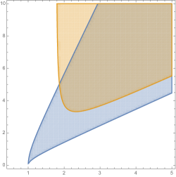
Figure 1: Tensor stability regions in the $(x,y)=(\delta,h)$ plane (for $h>0$); both for branch 2 (wedge, blue on line; for $\xi=10$), and for the self-accelerating solution (region above the upper curve, brown on line).

IX Study of vector perturbations and of their stability

IX.1 Symmetry of the gauge-fixed vector perturbation equations

We continue our study of cosmological perturbations in de Sitter-like TG solutions by considering the vector perturbations. While the tensor perturbations involved only three variables, the vector perturbations now involve seven (transverse vector) variables: one ($W_{a}$) in the vierbien perturbation, and six others ($\zeta_{a}$, $\nu_{a}$, $\mu_{a}$, $\kappa_{a}$, $A_{a}$ and $L_{a}$) in the connection perturbation.

Let us first mention that the system of vector equations has a certain symmetry that we have used as a check on our derivation. This symmetry is a residual symmetry after the (incomplete) gauge-fixing that we used. We have gauge-fixed the vector sector of the coordinate freedom by imposing the zero-shift condition (69). However, this condition will still be satisfied if we perform a time-independent helicity-1 spatial (infinitesimal) coordinate transformation $x^{\prime}{}^{\mu}=x^{\mu}+\xi^{\mu}$ with $\xi^{0}=0$ and $\xi^{a}_{C}=-C_{a}e^{i\mathbf{k}\cdot\mathbf{x}}$ (with $k^{a}C_{a}=0$). Such a diffeomorphism will act both on the vierbein and the connection as

$$-{\delta}_{\xi}e^{i}_{\mu}=\xi^{\lambda}\partial_{\lambda}e^{i}_{\mu}+\partial_{\mu}\xi^{\lambda}e^{i}_{{\lambda}}\,,$$ (169)

$$-{\delta}_{\xi}A_{ij\mu}=\xi^{\lambda}\partial_{\lambda}A_{ij\mu}+\partial_{\mu}\xi^{\lambda}A_{ij{\lambda}}\,.$$ (170)

As a consequence the spatial part of the vierbein will get out of the symmetric gauge (67). We must therefore apply an additional compensating infinitesimal Lorentz-rotation transformation $\omega_{ab}^{C}$ which is found to be (with $T_{[ab]}\equiv\frac{1}{2}(T_{ab}-T_{ba})$)

$$\omega_{ab}^{C}=ik_{[a}C_{b]}e^{i\mathbf{k}\cdot\mathbf{x}}\,.$$ (171)

Finally, the combined coordinate-plus-Lorentz transformation ${\delta}^{\rm tot}$ which preserves our gauge-fixing is found to act on the vierbein and the connection as (henceforth suppressing the $e^{i\mathbf{k}\cdot\mathbf{x}}$ factor, and denoting symmetrization as $T_{(ab)}\equiv\frac{1}{2}(T_{ab}+T_{ba})$)

$${\delta}^{\rm tot}e^{i}_{a}=ik_{(a}C_{i)}\,,$$ (172)

$${\delta}^{\rm tot}A_{\tilde{0}\tilde{a}b}=ife^{\phi}ik_{(b}C_{a)}\,,$$ (173)

$${\delta}^{\rm tot} \!\!A_{\tilde{a}\tilde{b}c}=k_{c}k_{[a}C_{b]}$$ (174)

$$+ \!\!ige^{\phi}\left(k_{c}\varepsilon_{abs}C^{s}+k_{[a}C_{p]}\varepsilon_{pbc}-k_{[b}C_{p]}\varepsilon_{pac}\right).$$

Using these formulas, we can compute how the above symmetry transforms the various vector variables parametrizing the perturbed vierbein and connection, e.g. we have: ${\delta}^{\rm tot}W_{a}=\frac{1}{2}C_{a}$. We can further decompose $C_{a}$ into its helicity pieces: $C^{a}=C_{(+1)}e_{+}^{a}+C_{(-1)}e_{-}^{a}$, and thereby derive separate symmetries of the helicity-$\pm 1$ variables given by

$${\delta}^{\rm tot}W_{(+1)}\!\! = \frac{1}{2}C_{(+1)}\,;\,{\delta}^{\rm tot}\nu_{(+1)}={\delta}^{\rm tot}\mu_{(+1)}=\frac{i}{2}fe^{\phi}C_{(+1)}\,;$$

$${\delta}^{\rm tot}L_{(+1)} = \frac{1}{2}gke^{\phi}C_{(+1)}\,;\,{\delta}^{\rm tot}\zeta_{(+1)}={\delta}^{\rm tot}\kappa_{(+1)}=0\,;$$

$${\delta}^{\rm tot}A_{(+1)} = \left(\frac{1}{2}-\frac{g}{k}e^{\phi}\right)C_{(+1)}\,.$$ (175)

We have checked that the vector perturbation equations we derived are invariant under these correlated shift symmetries of the vector variables.

IX.2 Reducing the vector perturbations to a linear system of three first-order ordinary differential equations

The obtention of the dispersion law for vector perturbations is more involved than the case discussed above of tensor perturbations. The first reason is that we have to deal with more variables: seven instead of three. As in the tensor case, the perturbations equations for helicity $+1$ decouple from those for helicity $-1$.

In all, one can derive ten vectorial equations from the gravitational and connection equations. However, we found that the helicity$\pm 1$ projections of the Bianchi identities of TG (explicitly worked out in Nikiforova:2017saf ) imply that there are (for each helicity) three identities among these equations. It is therefore sufficient to use only seven (independent) equations among the ten vector equations. It is also sufficient to deal only with the helicity $+1$ sector.

The seven, helicity $+1$, equations we worked with are given in Appendix B. As in the case of tensor perturbations, we use the rescaled field equations $\widehat{{\cal G}}_{ij}$, Eq. (96), and $\widehat{{\cal T}}_{[ij]k}$, Eq.(97). In addition, we scale out $k$ and use as independent variable $z=k\eta$. The notation in Appendix B is the following: there are four vectorial connection equations, which are denoted $V_{1}$, $V_{2}$, $V_{3}$, $V_{4}$, and three gravitational equations denoted $V_{5}$, $V_{6}$ and $V_{7}$. The vector helicity $+1$ variables entering these equations are respectively denoted (keeping close to the notation used for the corresponding vector variables $W_{a},\zeta_{a}$, etc.): $W_{1}$ ( $\equiv$ the helicity $+1$ component $W_{(1)}$ of $W_{a}$), $\zeta_{1}$, $\mu_{1}$, $\nu_{1}$, $\kappa_{1}$, $A_{1}$, and $L_{1}$.

First, we simplified these equations by replacing, respectively, $A_{1}$ and $\mu_{1}$ by the new variables $A_{3}$ and $\mu_{3}$ defined so that

$$A_{1}\equiv A_{3}-2L_{1}\,;\,\mu_{1}\equiv\mu_{3}+\nu_{1}\,.$$ (176)

In terms of these new variables, we find that, among the seven equations $V_{i}$, $i=1,\cdots 7$, four of them are algebraic in the four variables $\zeta_{1}$, $\nu_{1}$, $\kappa_{1}$ and $L_{1}$. More precisely $V_{2}$, $V_{5},$ $V_{6}$ and $V_{7}$ depend only on the variables

$$\zeta_{1}(z),\nu_{1}(z),\kappa_{1}(z),L_{1}(z)\,;$$ (177)

$$W_{1}(z),A_{3}(z),\mu_{3}(z)\,;\,W^{\prime}_{1}(z),A^{\prime}_{3}(z),\mu^{\prime}_{3}(z)\,.$$ (178)

When $h=g/{\lambda}\neq 0$ one finds that one can solve the set of four equations $\{V_{2}=0,V_{5}=0,V_{6}=0,V_{7}=0\}$ in the four variables $\{\zeta_{1}(z),\nu_{1}(z),\kappa_{1}(z),L_{1}(z)\}$, so as to get

$$\zeta_{1} =R_{\zeta}(z\,;\,W_{1},A_{3},\mu_{3}\,;\,W^{\prime}_{1},A^{\prime}_{3},\mu^{\prime}_{3}),$$ (179)

$$\nu_{1} =R_{\nu}(z\,;\,W_{1},A_{3},\mu_{3}\,;\,W^{\prime}_{1},A^{\prime}_{3},\mu^{\prime}_{3}),$$ (180)

$$\kappa_{1} =R_{\kappa}(z\,;\,W_{1},A_{3},\mu_{3}\,;\,W^{\prime}_{1},A^{\prime}_{3},\mu^{\prime}_{3}),$$ (181)

$$L_{1} =R_{L}(z\,;\,W_{1},A_{3},\mu_{3}\,;\,W^{\prime}_{1},A^{\prime}_{3},\mu^{\prime}_{3})\,.$$ (182)

Here, $R_{\zeta}$ etc. are linear functions of $W_{1},A_{3},\mu_{3}\,;\,W^{\prime}_{1},A^{\prime}_{3},\mu^{\prime}_{3}$ that are rational in $z$ (and the TG parameters).

In addition, the remaining three equations $V_{1},V_{3},V_{4}$ originally depended on the following set of variables

$$V_{1}:\; \zeta_{1},\nu_{1},\kappa_{1},L_{1}\,;\nu^{\prime}_{1}$$ (183)

$$W_{1},A_{3},\mu_{3}\,;\,W^{\prime}_{1},A^{\prime}_{3},\mu^{\prime}_{3}\,;$$ (184)

$$V_{3}:\; \zeta_{1},\nu_{1},\kappa_{1},L_{1}\,;\zeta^{\prime}_{1},\kappa^{\prime}_{1},L^{\prime}_{1}$$ (185)

$$W_{1},A_{3},\mu_{3}\,;\,A^{\prime}_{3}\,;\,\mu^{\prime\prime}_{3}\,;$$ (186)

$$V_{4}:\; \zeta_{1},\nu_{1},\kappa_{1},L_{1}\,;\nu^{\prime}_{1}$$ (187)

$$W_{1},A_{3},\mu_{3}\,;\,A^{\prime}_{3},\mu^{\prime}_{3}\,;\,A^{\prime\prime}_{3}\,.$$ (188)

When inserting the solutions (179) into the above equations $V_{1},V_{3},V_{4}$ (we denote the results as $\overline{V}_{1},\overline{V}_{3},\overline{V}_{4}$), one is a priori generating second derivatives of $W_{1},A_{3}$, and $\mu_{3}$. However, one finds that the coefficients of $A^{\prime\prime}_{3}$ and $\mu^{\prime\prime}_{3}$ actually vanish.

At this stage, we have three equations for three unknowns ($W_{1},A_{3},\mu_{3}$), depending on the following variables

$$\{\overline{V}_{1},\overline{V}_{3},\overline{V}_{4}\}:\;W_{1},A_{3},\mu_{3}\,;\,W^{\prime}_{1},A^{\prime}_{3},\mu^{\prime}_{3}\,;\,W^{\prime\prime}_{1}\,.$$ (189)

By algebraically combining these three equations, we can eliminate $W^{\prime\prime}_{1}$ in two of these equations. Actually, the third equation so obtained, namely a combination

$$\overline{V}_{4}^{\rm new}\equiv\overline{V}_{4}-C_{43}(z)\overline{V}_{3}\,,$$ (190)

which eliminates $W^{\prime\prime}_{1}$, is found to depend only on $W_{1},A_{3},\mu_{3}\,;\,W^{\prime}_{1}$, without involving the derivatives of $A_{3},\mu_{3}$. As a consequence we can combine $\overline{V}_{1}$ with the derivative of $\overline{V}_{4}^{\rm new}$ to eliminate $W^{\prime\prime}_{1}$ from our system of three equations. After these operations, we get a system of three equations involving only the variables

$$W_{1},A_{3},\mu_{3}\,;\,W^{\prime}_{1},A^{\prime}_{3},\mu^{\prime}_{3}\,.$$ (191)

This system is not quite our final system because one finds that it does not behave fully properly in the large-$z$ limit. However, if we replace the variable $\mu_{3}$ by the variable

$$\mu_{4}(z)\equiv\frac{\mu_{3}(z)}{z}\,,$$ (192)

one ends up with a system of three first-order equations in

$$\{y_{1},y_{2},y_{3}\}\equiv\{W_{1},A_{3},\mu_{4}\}\,,$$ (193)

which, when solved for first derivatives, yields a matrix system of the form

$$y_{i}^{\prime}(z)=m_{ij}(z)y_{j}(z)\,;\,i,j=1,2,3\,,$$ (194)

where the matrix $m_{ij}(z)$ has the same good property as the matrix obtained in the tensor case discussed above. Namely, the matrix $m_{ij}(z)$ has a finite limit, $m^{\infty}_{ij}$, as $z\to\infty$, and this limit yields a diagonalizable matrix. [This would not have been the case when keeping $\mu_{3}$.]

IX.3 Dispersion law for vector perturbations along the second branch of de Sitter-like solutions: necessary presence of gradient instabilities

We can then apply the same mathematical results Ince used in the tensor case above. The limiting system (with constant coefficients)

$$y_{i}^{\prime}(z)=m^{\infty}_{ij}\,y_{j}(z)\,,$$ (195)

where $m^{\infty}_{ij}=\lim_{z\to\infty}m_{ij}(z)$, will describe the large-$z$ asymptotics of our solutions (modulo power-law corrections). We therefore conclude that our solutions behave, for large$-z$, as a linear combination of eigensolutions of the type

$$y_{i}(z)=v_{i}e^{\sigma z}\,,$$ (196)

where $\sigma$ is one of the three eigenvalues of the $3\times 3$ matrix $m^{\infty}_{ij}$, and $v_{i}$ the corresponding eigenvector.

The problem of the stability of vector perturbations is thereby reduced to the purely algebraic question of computing the characteristic polynomial of the $3\times 3$ matrix $m^{\infty}_{ij}=\lim_{z\to\infty}m_{ij}(z)$. And the dispersion law for high-frequency vectorial modes is simply given by equating the latter characteristic polynomial to zero

$$P_{3}^{(h=+1)}(\sigma)=\det\left(m^{\infty}_{ij}-\sigma\delta_{ij}\right)\,.$$ (197)

The computation of the latter characteristic polynomial yields a cubic dispersion law of the form

$$\sigma(\sigma^{2}+c^{\rm vector})=0\,,$$ (198)

whose physical form (in terms of $\omega$ and $k$) was written in Eq. (114) above. As already announced, we found that the constant $c^{\rm vector}$ is given by

$$c^{\rm vector}=-\frac{({\delta}^{2}+h^{2}-1)^{2}}{4h^{2}}\,.$$ (199)

This dispersion law applies all along the second branch. Note that it depends neither on the parameter $\xi$ (which is independent from ${\delta}$ and $h$ along the second branch) nor on the parameter $c_{35}$ (which enters the vectorial perturbation equations).

The cubic dispersion law (198) has three roots: $\sigma=0$ and $\sigma=\pm\sqrt{-c^{\rm vector}}$. The vanishing root is a gauge mode which is already present in the flat space case (see below), and which corresponds to the shift symmetry by the constant vector $C^{a}$ discussed above. To have stability we would need to have only pure imaginary roots for $\sigma=i\omega/k$. This would require $c^{\rm vector}\geq 0$. However, we see that $-c^{\rm vector}$ is a square, so that we have the two real roots

$$\sigma=\pm\frac{({\delta}^{2}+h^{2}-1)}{2h}\,.$$ (200)

These real roots correspond to gradient instabilities (in the helicity $+1$ sector). The same roots are also present in the helicity $-1$ sector (together with the gauge mode $\sigma=0$).

The only way to avoid these (strong) gradient instabilities would be to tune the parameters of TG so that

$${\delta}^{2}+h^{2}=1\,;\,{\rm i.e.}\,f^{2}+g^{2}={\lambda}^{2}\,({\rm needed\,for\,stability})\,.$$ (201)

It is possible to tune $c_{6}$ and $c_{5}$ so as to satisfy the constraint (201). Indeed, if we impose

$$c_{5}=-16\,c_{6}\,,$$ (202)

Eqs. (55), (56), will imply the condition (201). One can see that there is a one-parameter family of such solutions, with ${\delta}$ varying between $\frac{1}{2}$ and $1$ (and $h^{2}$ correlatively varying between $\frac{3}{4}$ and $0$). However, the problem is that ${\delta}$ being always $\leq 1$ along this family of tuned solutions, the tensor dispersion law will necessarily be in the unstable region. Indeed, Fig. 1 (and the text around) showed that a necessary condition for tensor stability along the second branch is $\delta>1$. Note, in particular, that the self-accelerating solution itself was found to require ${\delta}>1.78078$ (see Eq. (167)) and cannot even be tuned to reach the values ${\delta}\leq 1$ needed for vector stability. This shows the necessary instability of the self-accelerating solution.

IX.4 Dispersion law for vector perturbations along the first branch of de Sitter-like solutions, and near the crossing between the two branches

It is finally interesting to consider the limit where the second branch of solutions approaches (and crosses) the first (torsionless) branch (along which ${\delta}=1$ and $h=0$). First, we note that the quantity $c^{\rm vector}$ entering the dispersion law (198) has a singular $\frac{0}{0}$ structure at its crossing with the first branch. If, however, we use the local expansion (151) for ${\delta}$ around this crossing, we find that the roots in $\sigma$ behave as

$$\sigma=\pm\frac{1-2a}{2}h+O(h^{3})\,.$$ (203)

The limit at $h\to 0$ does exist and corresponds to the dispersion law

$$\sigma^{3}=0\,;\,{\rm as}\,\,h\to 0\,{\rm(second\,branch)}\,.$$ (204)

Two remarks are in order here. On the one hand, the marginally stable dispersion law $\sigma^{3}=0$ (i.e. $\omega^{3}=0$) turns into a gradient instability as soon as $h\neq 0$, and, on the other hand, this differs from the dispersion law which holds all along the first branch, i.e. when $h=0$ and ${\delta}=1$.

We have computed the dispersion law along the first branch by using the same method as used along the second branch. This requires a separate computation because the presence of denominators $h^{2}$ in the second-branch dispersion law corresponds to the fact that the elimination of the algebraic variables $\{\zeta_{1}(z),\nu_{1}(z),\kappa_{1}(z),L_{1}(z)\}$ discussed above cannot be done in the same way. Indeed, one finds that the determinant entering the solution for these four variables vanishes when $h\to 0$. In the case (first branch) where $h=0$ from the start, one has to proceed slightly differently. One can, however, first eliminate the three variables $\{\zeta_{1}(z),\nu_{1}(z),\kappa_{1}(z)\}$. This yields four equations for the four unknowns $L_{1},W_{1},A_{3},\mu_{3}$. One then finds that, among the correspondingly reduced four remaining equations, there is an equation which is algebraic in $L_{1}$. One can then eliminate $L_{1}$ as a second step. This yields three equations for $W_{1},A_{3},\mu_{3}$. As before the latter system can be written as a first-order system of the same form as (195). Let us only cite here the resulting dispersion law along the first branch. It is found to be

$$\sigma(\sigma^{2}+1)=0\,.$$ (205)

Note that the latter dispersion law is: (i) stable (purely imaginary roots, apart from the gauge mode $\sigma=0$); and (ii) coincides with the (high-frequency limit of the) flat spacetime one, i.e.

$$\omega(\omega^{2}-{\mathbf{k}}^{2})=0\,.$$ (206)

The latter dispersion law is indeed the high-frequency limit of

$$\omega(\omega^{2}-{\mathbf{k}}^{2}-m_{2}^{2})=0\,,$$ (207)

(where $m_{2}$ denotes as above the mass of the massive spin-2 TG field) that describes, apart from the gauge mode $\omega=0$, the helicity-$+1$ projection of the massive spin-2 excitation, which is (together with its helicity-$-1$ counterpart) the only physical, propagating vector mode. [There are no physical vectorial degrees of freedom in the pure helicity-$\pm 2$ massless graviton.] The extra solution $\omega=0$ corresponds to the gauge-mode solution parametrized by $C^{a}$, discussed above.

Let us emphasize that the first-branch dispersion law (206) does not coincide with the $h\to 0$ limit of the dispersion law along the second branch. Indeed, $c^{\rm vector}_{B1}=-1$ along the first branch, while $\lim_{h\to 0}c^{\rm vector}_{B2}=0$, as a limit along the second branch.

This shows again that a torsionfull background (even an infinitesimal one) is a highly non trivial modification of the flat space dispersion laws in TG, which is prone to introducing instabilities that do not occur in torsionfree backgrounds.

X Study of scalar perturbations and of their stability

Finally, we come to the study of scalar perturbations and of their stability. We will be briefer than for the other perturbations, both because their treatment is similar to what we explained above for the tensor and vector perturbations, and because a detailed discussion of scalar perturbations has been recently given by one of us Nikiforova:2017saf ; Nikiforova:2017xww . We shall mainly comment on the differences between the present treatment and the one given in the latter references.

X.1 Deriving a linear system of four first-order ordinary differential equations from the ten scalar perturbations

As explained in Section V above, there are ten scalar variables: two, $\Phi,\Psi$, parametrize scalar perturbations of the vierbein, and eight, $\widetilde{\xi},\chi,\sigma,\rho,\theta,Q,u,M$, parametrize scalar perturbations of the connection. A difference with the treatment in Refs. Nikiforova:2017saf ; Nikiforova:2017xww is that the variables used there to parametrize perturbations were defined so as to parametrize the variations in the contorsion $K_{ij\mu}$ ($K$-parametrization), rather than in the connection $A_{ij\mu}$ ($A$-parametrization). This amounts to a conceptually unimportant redefinition of variables, involving some mixing between vierbein and connection variables. [We have checked that one gets the same final results using either the $K$-parametrization or the $A$-parametrization.] The precise connection between the variables denoted by the same letters as here in Refs. Nikiforova:2017saf ; Nikiforova:2017xww and the variables used here is

$$\sigma^{A}=\sigma^{K}\!-\partial_{\eta}\Psi\,;\,M^{A}=M^{K}\!-i\Psi\;;\,\widetilde{\xi}^{A}=\widetilde{\xi}^{K}\!-i\Phi\,.$$ (208)

As discussed in Refs. Nikiforova:2017saf ; Nikiforova:2017xww , the scalar projection of the perturbed field equations yields fourteen equations for the ten scalar variables. However, there are four Bianchi-like identities between these fourteen equations. This leaves one with ten independent equations for the ten scalar unknowns. We give in Appendix C the ten independent scalar equations we have used, expressed in terms of our current $A$-parametrized variables, and in terms of rescaled parameters (and unknowns) and of the variable $z=k\eta$. [We do not put a superscript $A$ on our variables.]

Actually, following Refs. Nikiforova:2017saf ; Nikiforova:2017xww , we shall work with suitable combinations of the equations in Appendix C and of their derivatives. Indeed, two (and only two) among the equations given in Appendix C contain second derivatives of scalar variables (namely the eighth equation, which involves $\chi^{\prime\prime}$, and the ninth, which involves $\rho^{\prime\prime}$). However, by suitable combinations of the equations and their derivatives one can replace the latter two equations by two other equations involving (as the eight other ones) only first derivatives of the scalar variables. At this stage, we have therefore a system of ten equations which involve at most the first derivatives of the scalar variables. In a second stage, we can combine equations of the latter system so as to define two combinations that are purely algebraic, i.e. that involve no derivatives. [The explicit expressions of these two algebraic equations have been given in Nikiforova:2017saf . By using the transformations (208) above, one can reexpress them in terms of our $A$-parametrization variables.] At this second stage, we have therefore eight equations, say $E_{1},E_{2},\cdots,E_{8}$, involving first derivatives and two algebraic equations, say $AE_{1},AE_{2}$, involving no derivatives. We then found convenient to deal with this system of equations in the following way (which differs both from the methods used above, and from the one used in Refs. Nikiforova:2017saf ; Nikiforova:2017xww ).

First, we redefine our scalar variables as follows, and separate them in two different groups, denoted $y_{I}$ with $I=1,2,\cdots,6$ and $y_{A}$, with $A=7,8,9,10$:

$$\{y_{I}\}_{I=1,\cdots,6}:y_{1} = \Psi\,;\,y_{2}=z^{-1}\chi\,;\,y_{3}=Q\,;$$

$$\,y_{4} = u\,;\,y_{5}=M\,;y_{6}=\rho\,;$$ (209)

where the $z$-dependent rescaling of $\chi$ is necessary to end up with a differential-coefficient matrix $m_{ij}(z)$ having a finite limit when $z\to\infty$, and

$$\{y_{A}\}_{A=7,\cdots,10}:y_{7}=\sigma\,;\,y_{8}=\xi\,;\,y_{9}=\Phi\,;\,y_{10}=\theta\,.$$ (210)

This separation in two groups is linked to the following facts Nikiforova:2017saf : the variables of the second group enter equations $E_{1},E_{2},\cdots,E_{8}$ only algebraically, and do not enter the two algebraic equations $AE_{1},AE_{2}$, which only involve the variables of the first group.

As a consequence of the latter facts, we can usefully consider the following system of twelve equations

$$E_{1}(y_{A},y_{I},y^{\prime}_{I}) = 0\,;\cdots;\,E_{8}(y_{A},y_{I},y^{\prime}_{I})=0\,;$$

$$AE_{1}(y_{I}) = 0\,;\,AE_{2}(y_{I})=0\,;\,$$

$$\left(\frac{d}{dz}AE_{1}\right)(y_{I},y^{\prime}_{I}) = 0\,;\,\left(\frac{d}{dz}AE_{2}\right)(y_{I},y^{\prime}_{I})=0\,.$$

These twelve equations define a system of equations for the following twelve unknowns:

$$\{y^{\prime}_{1},y^{\prime}_{2},y^{\prime}_{3},y^{\prime}_{4},y^{\prime}_{5},y^{\prime}_{6},y_{5},y_{6},y_{7},y_{8},y_{9},y_{10}\}\,.$$ (212)

We find that this linear system of twelve equations for twelve unknowns is uniquely solvable, and thereby allows one to express the twelve quantities (212) in terms of the remaining variables occurring in the system, namely $\{y_{1},y_{2},y_{3},y_{4}\}$. In other words, we have thereby not only succeeded in algebraically expressing $\{y_{5},y_{6},y_{7},y_{8},y_{9},y_{10}\}$ in terms of $\{y_{1},y_{2},y_{3},y_{4}\}$ (thereby showing that six scalar variables can be algebraically eliminated), but, most importantly, we have also expressed the derivatives $\{y^{\prime}_{1},y^{\prime}_{2},y^{\prime}_{3},y^{\prime}_{4}\}$ in terms of $\{y_{1},y_{2},y_{3},y_{4}\}$. In other words, we have obtained the following autonomous system of four first-order equations for the four unknowns $\{y_{1},y_{2},y_{3},y_{4}\}$:

$$y^{\prime}_{i}=m_{ij}(z)y_{j}\,;\,{\rm where}\,i,j=1,2,3,4\,.$$ (213)

X.2 Dispersion law for scalar perturbations

The system (213) is the analog of the tensor and vector systems (124), (194). Thanks to our redefinition of the variable $y_{2}$, we find that the $4\times 4$ coefficient matrix $m_{ij}(z)$ entering this system has a finite limit at $z\to\infty$. As before, we conclude that the dispersion law for scalar perturbations is given by the characteristic polynomial of the $4\times 4$ coefficient matrix $m^{\infty}_{ij}=\lim_{z\to\infty}m_{ij}(z)$, say

$$P_{4}^{\rm tensor}(\sigma)\equiv\det\left(m^{\infty}_{ij}-\sigma\delta_{ij}\right);\,i,j=1,2,3,4\,.$$ (214)

The explicit computation of this scalar dispersion law is found to be

$$P_{4}^{\rm scalar}(\sigma)=\sigma^{2}\left(\sigma^{2}+c^{\rm scalar}({\delta},h,c_{35})\right)\,,$$ (215)

i.e., in terms of $\omega$ and $k$,

$$\omega^{2}\left(\omega^{2}-c^{\rm scalar}{\mathbf{k}}^{2}\right)=0\,.$$ (216)

The quantity $c^{\rm scalar}$ is found to be given by the complicated expression

$$c^{\rm scalar}({\delta},h,c_{35})=\frac{N^{\rm scalar}}{D^{\rm scalar}}\,,$$ (217)

with

$$N^{\rm scalar}=-\Big{\{}9(1-2{\delta})^{2}h^{2}(-5+4{\delta}+4{\delta}^{2}+4h^{2})$$

$$+3c_{35}(-1+2{\delta})\big{[}-3{\delta}^{5}+3{\delta}^{6}+17h^{2}+2h^{4}-3h^{6}$$

$$+3{\delta}^{4}(-2+h^{2})+{\delta}^{3}(6+26h^{2})$$

$$+{\delta}^{2}(3+4h^{2}-3h^{4})+{\delta}(-3-38h^{2}+29h^{4})\big{]}$$

$$+2c_{35}^{2}\big{[}-13{\delta}^{6}+6{\delta}^{7}+21{\delta}^{4}h^{2}+{\delta}^{5}(7+6h^{2})$$

$$+{\delta}^{3}(4-34h^{2}-6h^{4})-h^{2}(7+8h^{2}+h^{4})$$

$$+{\delta}^{2}(-7-8h^{2}+33h^{4})+{\delta}(3+28h^{2}+7h^{4}-6h^{6})\big{]}\Big{\}}\,,$$ (218)

and

$$D^{\rm scalar}=(-3+2{\delta}^{2}+2h^{2})\Big{\{}9(1-2{\delta})^{2}h^{2}$$

$$+12c_{35}(1-2{\delta})^{2}h^{2}+4c_{35}^{2}\big{[}-2{\delta}^{3}$$

$$+{\delta}^{4}+h^{2}-2{\delta}h^{2}+h^{4}+{\delta}^{2}(1+2h^{2})\big{]}\Big{\}}\,.$$ (219)

[As a numerical check on the above expressions, note that $c^{\rm scalar}(1,2,3)=-13/25$, corresponding to $N^{\rm scalar}=-3276$, and $D^{\rm scalar}=6300$.]

Several remarks are in order concerning this scalar dispersion law. Let us first emphasize again that Eq. (215) gives the scalar dispersion law all along the second branch of solutions (i.e. without assuming that $\xi$ is related to ${\delta}$ and $h$). Therefore, it could a priori depend not only on the background-solution parameters ${\delta}$ and $h$ but also on $\xi$ (as had happened for the tensor dispersion law, Eq. (147)). However, it happens not to depend on $\xi$. [More precisely, one finds that, when expanding the characteristic polynomial of $m_{ij}(z)$ in inverse powers of $z$, the value of $\xi$ starts affecting the evolution of the scalar perturbations only at order $O(1/z^{2})$.] On the other hand, contrary to the previous (tensor and vector) dispersion laws, it depends on a TG parameter that did not enter the previous dispersion laws, namely $c_{35}\equiv c_{3}/c_{5}$. Let us remark that the scalar dispersion law derived here, Eq. (215), has the same general structure as the result obtained in Ref. Nikiforova:2017xww , which had studied, like here, the case where the torsion background is comparable to the Hubble scale, i.e. the case where both ${\delta}$ and $h$ are of order unity. [One cannot directly compare with the previous result of Ref. Nikiforova:2017saf which had considered a parametrically different case.] However, the specific value of the constant $c^{\rm scalar}$ derived here differs from the (simpler) value, namely $c^{\rm scalar}_{N}=2{\delta}+1$, given there (see the $\Lambda\to 0$ limit of Eq. (33) in Ref. Nikiforova:2017saf ). A reexamination of the derivation in Ref. Nikiforova:2017saf has allowed us to locate a coding misprint. After correcting it, it was found that the method used in Ref. Nikiforova:2017saf leads to the value of $c^{\rm scalar}$ given in Eq. (217) above. Note that this qualifies the conclusion of Ref. Nikiforova:2017saf that the scalar perturbations have no exponential instabilities. Actually, as we shall show next the quantity $c^{\rm scalar}({\delta},h,c_{35})$ is positive in part of the parameter space (corresponding to stability), but negative in other regions (where there are gradient instabilities).

Let us also emphasize a significant difference between the dispersion law Eq. (216) and the dispersion law for scalar perturbations along torsionless backgrounds. As already mentioned in Sec. VII, the latter dispersion law is

$$\left(\omega^{2}-{\mathbf{k}}^{2}\right)\left(\omega^{2}-{\mathbf{k}}^{2}\right)=0\,,$$ (220)

where the two factors $\omega^{2}-{\mathbf{k}}^{2}$ describe the propagation of the two helicity-0 d.o.f. (one being part of the massive spin-2 field, the other being a pseudo-scalar torsion-related field). By comparing with Eq. (216), we see that while two modes that propagated at the speed of light around a torsionless background now propagate at the modified velocity $\sqrt{c^{\rm scalar}}$ (when it is real), two other modes that propagated at the velocity of light now propagate with zero velocity (factor $\omega^{2}$ instead of $\omega^{2}-{\mathbf{k}}^{2}$). This shows again the drastic effect of having a torsionfull background.

Let us emphasize that the dispersion constant $c^{\rm scalar}({\delta},h,c_{35})$ has the same $\frac{0}{0}$ structure near torsionfree backgrounds that we found above for tensor and vector dispersion laws. Indeed, it is easily checked that, when ${\delta}\to 1$ and $h\to 0$ both the numerator $N^{\rm scalar}$ and the denominator $D^{\rm scalar}$ tend to zero. However, if we consider the specific limit (151) corresponding to approaching the torsionfree case along the second branch, we find the following limiting behavior

$$c^{\rm scalar}({\delta},h,c_{35})=3+2\frac{15-36a+16c_{35}-18ac_{35}}{3+2c_{35}}h^{2}+O(h^{4})$$ (221)

We therefore have tensor stability ($c^{\rm scalar}>0$, see next subsection) in the vicinity of torsionfree backgrounds. However, we do not have a continuous behavior of the helicity-0 dispersion law in the vicinity of torsionfree backgrounds. Indeed, the limit of the torsionfull dispersion law (216) as ${\delta}\to 1$ and $h\to 0$ is $\omega^{2}\left(\omega^{2}-3{\mathbf{k}}^{2}\right)=0$, instead of $\left(\omega^{2}-{\mathbf{k}}^{2}\right)\left(\omega^{2}-{\mathbf{k}}^{2}\right)=0$.

X.3 Regions of parameter space where scalar perturbations (along the second branch) are stable

In view of the dispersion law (216), the condition for the stability of scalar perturbations is

$$c^{\rm scalar}({\delta},h,c_{35})>0\,.$$ (222)

As we found above that there were necessary instabilities in the vector sector, it is not worth discussing in full detail which regions of parameter space lead to stability in the scalar sector. Let us only say that, for each given value of $c_{35}$, there is an infinite region of the ${\delta},h$ plane where there are no exponential scalar instabilities. The shape of the stable region remains qualitatively similar, though it undergoes very significant quantitative changes, as $c_{35}$ varies. Let us only give one specific example of stability region in the ${\delta},h$ plane, namely the one corresponding to the specific case $c_{35}=-2$. The corresponding scalar stability region in the ${\delta},h$ plane (for the second branch) is shown (blue on line) in Fig. 2. When restricting our attention to the self-accelerating solution, we must further restrict the parameters by the inequality $h^{2}>{\delta}^{2}+{\delta}$, Eq. (60). Restricting to the region above the hyperbola $h^{2}-{\delta}^{2}-{\delta}=0$ (displayed as brown on line) cuts off part of the previous stability region, as shown in Fig. 2.

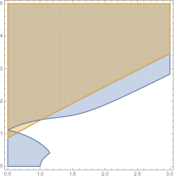
Figure 2: Scalar stability regions (for $c_{35}=-2$) in the $(x,y)=(\delta,h)$ plane (for $h>0$); both for branch 2 (blue region on line), and for the self-accelerating solution (part of the previous region above the line $h^{2}={\delta}^{2}+{\delta}$, shown as brown on line).

XI Conclusions

We have studied linearized perturbations of de Sitter-like solutions in a class of geometric theories (called Torsion Gravity, or TG) that generalize General Relativity by including a propagating torsion in addition to the usual Einsteinian metric. The class of TG theories we considered contains six parameters, including a vacuum-energy parameter $c_{2}$. When considered either on a flat background (when taking $c_{2}=0$), or on a torsionfree de Sitter background (when $c_{2}\neq 0$), these theories were found in previous work to be ghost-free and tachyon-free, and to feature, as propagating fields, both massive spin-2 and massive spin-0 excitations, in addition to the Einsteinian massless spin-2 field.

We considered the two different branches of de Sitter-like solutions admitted by this class of TG theories. The exponential expansion of the first branch of solutions (which had already been studied in Nair:2008yh ) is sustained by the vacuum energy $c_{2}$, and these solutions have zero torsion. On the other hand, the second branch of solutions has a non-zero torsion, and its exponential expansion is jointly sustained by its torsion background and by the vacuum-energy parameter $c_{2}$. This second branch can interpolate between a torsion-free background, and a self-accelerating torsionfull solution Nikiforova:2016ngy whose expansion is entirely sustained by the torsion background (with $c_{2}=0$). We contrasted the properties of the cosmological perturbations in these two branches of solutions as a way to understand the influence of a torsion background on the stability of the de Sitter-like solutions.

The main new finding of the present paper is that the presence of a torsion background (and even an infinitesimal one) generically creates gradient instabilities in the vector sector of the cosmological perturbations. See Eqs. (198), (199). No tuning of the TG parameters can kill these instabilities without creating instabilities in the other sectors. We have also studied the cosmological perturbations in the tensor and scalar sectors. The tensor sector has no exponential instabilities if the quantity $b^{\prime}_{\rm tensor}-1$, Eq. (147) is positive. We found that this will be the case in a large region of the TG parameter space. Along a general solution of the second branch the tensor-stability region in the plane of ${\delta}=-f/{\lambda}$ and $h=g/{\lambda}$ depends also on the theory parameter $\xi={\overline{\alpha}}/{\widetilde{\alpha}}$. It is illustrated in Fig. 1 for the value $\xi=10$. The tensor-stability region for the self-accelerating solution (with $c_{2}=0$) covers also a large part of the ${\delta},h$ plane. See Eq. (168) and Fig. 1. We finally discussed the stability of scalar perturbations. Like tensor perturbations, scalar perturbations were found to have no exponential instabilities in a large part of parameter space, defined by $c^{\rm scalar}>0$ with $c^{\rm scalar}$ defined in Eqs. (217), (X.2), (X.2). The scalar-stability region depends on three parameters: ${\delta},h$ and $c_{35}$. It is illustrated (both for the general second branch and for the self-accelerated solution) in the specific case $c_{35}=-2$ in Fig. 2.

In the course of our study we compared and contrasted the (linearized) (in)stability of torsionfull de Sitter-like solutions to the (linearized) stability Nair:2008yh ; Nikiforova:2009qr of torsionfree solutions. This comparison showed the drastic effect on stability of having a nonzero torsion background. While torsionfree backgrounds exhibited (in the high-frequency limit) the same dispersion laws as flat spacetime, the presence of even an infinitesimal torsion background drastically affected the dispersion law by introducing, in the dispersion laws, quantities having a $\frac{0}{0}$ structure in the vanishing torsion limit. This structure is connected with some discontinuities (as the torsion goes to zero) in the dispersion laws. Only the tensor dispersion law has no discontinuity between a torsionfree background (first branch) and a torsionfull one with infinitesimal torsion. The common limit of the (high-frequency) dispersion law is $(\omega^{2}-{\mathbf{k}}^{2})^{2}=0$. By contrast, while the torsionfree dispersion law for vector perturbations is $\omega(\omega^{2}-{\mathbf{k}}^{2})=0$, the corresponding vector dispersion law around an infinitesimal torsion background becomes $\omega^{3}=0$. Similarly, while the torsionfree dispersion law for scalar perturbations is $(\omega^{2}-{\mathbf{k}}^{2})^{2}=0$, the corresponding scalar dispersion law around an infinitesimal torsion background becomes $\omega^{2}(\omega^{2}-3{\mathbf{k}}^{2})=0$. These discontinuous differences with the dispersion laws for linearized perturbations around a torsion-free background are linked with the presence of instability-related $\frac{0}{0}$ structures in the perturbations around both torsionfull and torsionless backgrounds. Indeed, at the crossing between the two branches, the quantity $1+4\widehat{c}_{5}$ vanishes, see Eq. (153), and this corresponds to the vanishing of the quantity $c_{5}\kappa$ that is crucially related to the stability of the torsionless branch (see notably Eqs. (9), (11), (22), and (30) in Ref. Nikiforova:2009qr ).

The overall conclusion of the present work is that a torsionfull background is a highly non trivial modification of the propagation properties of perturbations in TG. Further work is needed to see if generic torsionfull backgrounds are prone to introducing instabilities, or if the instabilities we found are mainly due to the (generalized) self-accelerating nature of the special de Sitter backgrounds we considered. There is, however, the good news that in all cases, and in spite of significant modifications in the algebraic structure of the equations for perturbations, the presence of a torsion background left intact the number of propagating degrees of freedom. In other words, TG seems to be insensitive to the Boulware-Deser-type instability phenomenon Boulware:1973my that generally affects theories containing a massive spin-2 excitation.

Appendix A Tensor perturbation equations

As explained in Sec. V above, there are three tensor perturbations: $\pi_{ab}$ in the vierbein perturbation, and $\tau_{ab}$ and $N_{ab}$ in the connection perturbation. To get equations for the coupled propagation of the three tensor excitations $\pi_{ab}$, $\tau_{ab}$ and $N_{ab}$, we must consider which equations among the perturbations of the full (rescaled) field equations (i.e. the $O(\gamma)$ contributions in $\widehat{{\cal G}}_{ij}$, Eq. (96), and $\widehat{{\cal T}}_{[ij]k}$, Eq.(97)) contain such tensor contributions. Denoting spatial indices as $a,b,c,d=1,2,3$, one easily sees that there are only three “two-index” rescaled equations, namely $\widehat{{\cal G}}_{ab}$, $\widehat{{\cal T}}_{0ab}$ and the dualized version of $\widehat{{\cal T}}_{abc}$, i.e. $\widehat{{\cal T}}^{*}_{dc}\equiv\varepsilon_{abd}\widehat{{\cal T}}_{abc}$, which can provide three tensor equations for our three tensor unknowns $\pi_{ab}$, $\tau_{ab}$ and $N_{ab}$.

The next step is to decompose these tensor equations into their helicity $\pm 2$ components. When doing so, we indeed found that the latter three equations do contain helicity $\pm 2$ irreducible pieces constraining the propagation of the three tensor excitations. We recall that the helicity $\pm 2$ components of any two-index tensor are defined so that, for instance, $\pi_{ab}=\pi_{(+2)}e_{+}^{ab}+\pi_{(-2)}e_{-}^{ab}$ (where we defined $e_{+}^{ab}\equiv e_{+}^{a}e_{+}^{b}$), or $\widehat{{\cal G}}_{ab}=\widehat{{\cal G}}_{(+2)}e_{+}^{ab}+\widehat{{\cal G}}_{(-2)}e_{-}^{ab}+{\rm lower\,helicities}$. [A non-symmetric two-index tensor, such as $\widehat{{\cal G}}_{ab}$, does not even need to be explicitly symmetrized over $ab$ to be decomposed into helicity-$\pm 2$ components because its antisymmetric part, being dual to a vector, will not contain any helicity-$\pm 2$ piece.]

We extracted the helicity $\pm 2$ components of the expressions $\widehat{{\cal G}}_{(ab)}$, $\widehat{{\cal T}}_{0(ab)}$ and $\widehat{{\cal T}}^{*}_{(ab)}$ by inserting the helicity decompositions of $\pi_{ab}$, $\tau_{ab}$ and $N_{ab}$ in these expressions. Then, the use of coding rules to express the pure-helicity character of $e_{\pm}^{ab}$ allows one to extract the coefficients of $e_{\pm}^{ab}$ in the equations. An alternative (equivalent) way would have been to contract the live tensor indices of the above mentioned two-index tensor equations by $\frac{1}{4}e_{-}^{ab}$ (to get the equations for the helicity-$+2$ components), or by $\frac{1}{4}e_{+}^{ab}$ (to get the equations for the helicity-$+2$ components). We use here the fact that $e_{+}^{a}$ and $e_{-}^{a}$ are null vectors ($e_{+}^{a}e_{+}^{a}=0$, $e_{-}^{a}e_{-}^{a}=0$) having as only nonzero scalar product among $e_{+}^{a}$, $e_{-}^{a}$ and $k^{a}$ their mutual product: $e_{+}^{a}e_{-}^{a}=2$.

After this helicity decomposition, we get, on the one hand, three coupled equations for the helicity $+2$ variables, $\pi_{(+2)}$, $\tau_{(+2)}$ and $N_{(+2)}$, and, on the other hand, three coupled equations for the helicity $-2$ variables, $\pi_{(-2)}$, $\tau_{(-2)}$ and $N_{(-2)}$. The two types of helicity do not mix between themselves, and the helicity $-2$ system is seen to be obtained from the helicity $+2$ one simply by changing $g\to-g$. The two latter facts are simple consequences of the structure of the field equations. In particular, as $g$ enters the background in the combination $g\varepsilon_{abc}$, the sign flip $g\to-g$ does correspond to a different choice for the orientation of space, which indeed reflects as an exchange between the two helicities, see Eqs. (V).

Denoting (as in our code) $\pi_{(+2)}$ by $K_{1}$, $\tau_{(+2)}$ by $F_{1}$, and $N_{(+2)}$ by $N_{1}$, and introducing the rescaled variables, $F_{n}\equiv k^{-1}\tau_{(+2)}$, and $i\,N_{n}\equiv N_{(+2)}$, we found that the first-order ($O(\gamma)$) perturbations of, respectively, $\widehat{{\cal T}}_{0ab}$, $\widehat{{\cal T}}^{*}_{dc}$ and $\widehat{{\cal G}}_{ab}$ yield, using the above-defined extraction procedure, three (rescaled) equations, respectively denoted $\widehat{E}_{1}=0$, $\widehat{E}_{3}=0$ and $\widehat{E}_{5}=0$, for $K_{1}$, $F_{n}$ and $N_{n}$, with

$$\widehat{E}_{1}\equiv(-\frac{3\,z}{2}-3\,{\widehat{c}_{5}}\delta\,z-3\,{\widehat{c}_{5}}\delta^{2}z)\,F_{n}$$

$$+(\frac{3\,\delta}{2}-6\,{\widehat{c}_{5}}\delta+3\,{\widehat{c}_{5}}\delta^{2}+3\,{\widehat{c}_{5}}\delta^{3}+6\,{\widehat{c}_{5}}h^{2}+48\,{\widehat{c}_{6}}h^{2}-3\,{\widehat{c}_{5}}\delta h^{2}+96\,{\widehat{c}_{6}}\delta h^{2}+48\,{\widehat{c}_{6}}h\,z+96\,{\widehat{c}_{6}}\delta h\,z)\,K_{1}$$

$$+(3\,{\widehat{c}_{5}}h\,z+48\,{\widehat{c}_{6}}h\,z-3\,{\widehat{c}_{5}}\delta h\,z+96\,{\widehat{c}_{6}}\delta h\,z+3\,{\widehat{c}_{5}}\delta\,z^{2})\,N_{n}$$

$$+(-\frac{3\,z}{2}+3\,{\widehat{c}_{5}}\delta\,z-3\,{\widehat{c}_{5}}\delta^{2}z+3\,{\widehat{c}_{5}}h^{2}z)\,\partial_{z}K_{1}+(-3\,{\widehat{c}_{5}}h\,z^{2}+3\,{\widehat{c}_{5}}z^{3})\,\partial_{z}N_{n}+3\,{\widehat{c}_{5}}z^{3}\,\partial^{2}_{z}F_{n}\;,$$ (223)

$$\widehat{E}_{3}\equiv(-3\,h-18\,{\widehat{c}_{5}}\delta h+96\,{\widehat{c}_{6}}\delta h-6\,{\widehat{c}_{5}}\delta^{2}h+192\,{\widehat{c}_{6}}\delta^{2}h+6\,{\widehat{c}_{5}}h^{3}-3\,z-6\,{\widehat{c}_{5}}\delta\,z+6\,{\widehat{c}_{5}}\delta^{2}z-6\,{\widehat{c}_{5}}h^{2}z)\,K_{1}$$

$$+(-96\,{\widehat{c}_{6}}h\,z+6\,{\widehat{c}_{5}}\delta h\,z-192\,{\widehat{c}_{6}}\delta h\,z-6\,{\widehat{c}_{5}}\delta\,z^{2})\,F_{n}+(-3\,z-12\,{\widehat{c}_{5}}\delta\,z+6\,{\widehat{c}_{5}}h^{2}z-12\,{\widehat{c}_{5}}h\,z^{2}+6\,{\widehat{c}_{5}}z^{3})\,N_{n}$$

$$+(-6\,{\widehat{c}_{5}}h\,z^{2}+6\,{\widehat{c}_{5}}z^{3})\,\partial_{z}F_{n}-(96\,{\widehat{c}_{6}}h\,z+192\,{\widehat{c}_{6}}\delta h\,z)\,\partial_{z}K_{1}\;,$$ (224)

$$\widehat{E}_{5}\equiv(\frac{3\,\delta\,z}{2}+3\,{\widehat{c}_{5}}\delta^{2}z-3\,{\widehat{c}_{5}}\delta^{3}z+48\,{\widehat{c}_{6}}h^{2}z+3\,{\widehat{c}_{5}}\delta h^{2}z+96\,{\widehat{c}_{6}}\delta h^{2}z-48\,{\widehat{c}_{6}}h\,z^{2}-96\,{\widehat{c}_{6}}\delta h\,z^{2})\,F_{n}$$

$$+(\frac{3\,h\,z}{2}+3\,{\widehat{c}_{5}}\delta h\,z-48\,{\widehat{c}_{6}}\delta h\,z-3\,{\widehat{c}_{5}}\delta^{2}h\,z-96\,{\widehat{c}_{6}}\delta^{2}h\,z+3\,{\widehat{c}_{5}}h^{3}z-\frac{3\,z^{2}}{2}-3\,{\widehat{c}_{5}}\delta\,z^{2}+3\,{\widehat{c}_{5}}\delta^{2}z^{2}-3\,{\widehat{c}_{5}}h^{2}z^{2})\,N_{n}$$

$$+(-\frac{3\,\delta}{2}-\frac{3\,\delta^{2}}{2}+3\,{\widehat{c}_{5}}\delta^{2}-6\,{\widehat{c}_{5}}\delta^{3}+3\,{\widehat{c}_{5}}\delta^{4}+\frac{3\,h^{2}}{2}-48\,{\widehat{c}_{6}}h^{2}+6\,{\widehat{c}_{5}}\delta h^{2}-192{\widehat{c}_{6}}\delta h^{2}-6\,{\widehat{c}_{5}}\delta^{2}h^{2}$$

$$-192\,{\widehat{c}_{6}}\delta^{2}h^{2}+3\,{\widehat{c}_{5}}h^{4}+\frac{3\,z^{2}\xi}{2})\,K_{1}+(-\frac{3}{2}z^{2}+3\,{\widehat{c}_{5}}\delta\,z^{2}-3\,{\widehat{c}_{5}}\delta^{2}z^{2}+3\,{\widehat{c}_{5}}h^{2}z^{2})\,\partial_{z}F_{n}$$

$$-3\,z\xi\partial_{z}K_{1}+(48\,{\widehat{c}_{6}}h\,z^{2}+96\,{\widehat{c}_{6}}\delta h\,z^{2})\,\partial_{z}N_{n}+\frac{3}{2}z^{2}\xi\,\partial^{2}_{z}K_{1}\;.$$ (225)

Appendix B Vector perturbation equations

We extracted seven vector perturbations equations for the various helicity-$+1$ components $W_{1}$ ( $\equiv$ the helicity $+1$ component $W_{(1)}$ of $W_{a}$), $\zeta_{1}$, $\mu_{1}$, $\nu_{1}$, $\kappa_{1}$, $A_{1}$, and $L_{1}$ of the vector perturbations in the following way. As in the tensor case, we start from the $O(\gamma)$ pieces in the rescaled field equations $\widehat{{\cal T}}_{[ij]k}$, Eq.(97), and $\widehat{{\cal G}}_{ij}$, Eq. (96). We use the same extraction procedure as above, except that we decompose now any vectorial equation into, e.g. $\widehat{{\cal G}}_{a0}=\widehat{{\cal G}}_{(+1)}e_{+}^{a}+\widehat{{\cal G}}_{(-1)}e_{-}^{a}$. Equations containing more than one index are conveniently dualized into vectorial equations. We so derived four helicity-$+1$ equations (denoted $V_{1}$ to $V_{4}$) from the connection field equations, and three other equations (denoted $V_{5}$ to $V_{7}$) from the gravity field equations. In these equations, we have everywhere eliminated the TG basic coefficient $c_{4}$ by using the constraint $c_{4}=-c_{3}-3c_{5}$. In addition, several vector variables have been rescaled as follows: $W_{1}^{\rm new}=kW_{1};A_{1}^{\rm new}==kA_{1};\zeta_{1}^{\rm new}=k^{-1}\zeta_{1};L_{1}^{\rm new}=k^{-1}L_{1}$. We henceforth skip the superscripts “new”.

The explicit forms of the left-hand sides of the seven helicity-$+1$ equations $V_{1}=0$ to $V_{7}=0$ are listed below (with the field equation from which they were extracted)

Equation $\widehat{{\cal T}}_{[a0]0}\to V_{1}$:

$$(\frac{3z}{2}+2{\widehat{c}_{3}}h^{2}z-3{\widehat{c}_{5}}h^{2}z-{\widehat{c}_{3}}hz^{2}-2{\widehat{c}_{3}}z\,\delta^{2})A_{1}+(3z+4{\widehat{c}_{3}}h^{2}z-6{\widehat{c}_{5}}h^{2}z-{\widehat{c}_{3}}z^{3}-4{\widehat{c}_{3}}z\,\delta^{2})L_{1}$$

$$+(-\frac{3z}{2}+3{\widehat{c}_{5}}h^{2}z+3{\widehat{c}_{5}}z\,\delta-3{\widehat{c}_{5}}z\,\delta^{2})W_{1}+(4{\widehat{c}_{3}}h^{2}z+6{\widehat{c}_{5}}h^{2}z-4{\widehat{c}_{3}}hz^{2}-6{\widehat{c}_{5}}hz^{2}+{\widehat{c}_{3}}z^{3}-4{\widehat{c}_{3}}z\,\delta^{2})\zeta_{1}$$

$$+(8i\,{\widehat{c}_{3}}hz\,\delta+6i\,{\widehat{c}_{5}}hz\,\delta-4i\,{\widehat{c}_{3}}z^{2}\delta-3i\,{\widehat{c}_{5}}z^{2}\delta)\kappa_{1}+(48i\,{\widehat{c}_{6}}hz+4i\,{\widehat{c}_{3}}hz\,\delta+9i\,{\widehat{c}_{5}}hz\,\delta+96i\,{\widehat{c}_{6}}hz\,\delta-i\,{\widehat{c}_{3}}z^{2}\delta)\mu_{1}$$

$$+(-48i\,{\widehat{c}_{6}}hz-4i\,{\widehat{c}_{3}}hz\,\delta-9i\,{\widehat{c}_{5}}hz\,\delta-96i\,{\widehat{c}_{6}}hz\,\delta-i\,{\widehat{c}_{3}}z^{2}\delta-3i\,{\widehat{c}_{5}}z^{2}\delta)\nu_{1}+2{\widehat{c}_{3}}z^{2}\delta\,\partial_{z}A_{1}$$

$$+4{\widehat{c}_{3}}z^{2}\delta\,\partial_{z}L_{1}+(-2i\,{\widehat{c}_{3}}hz^{2}-3i\,{\widehat{c}_{5}}hz^{2}+i\,{\widehat{c}_{3}}z^{3})\,\partial_{z}\mu_{1}+(2i\,{\widehat{c}_{3}}hz^{2}+3i\,{\widehat{c}_{5}}hz^{2}-i\,{\widehat{c}_{3}}z^{3}-3i\,{\widehat{c}_{5}}z^{3})\,\partial_{z}\nu_{1}\;.$$ (226)

Equation $\varepsilon^{abc}\widehat{{\cal T}}_{[ab]0}\to V_{2}$:

$$z(96{\widehat{c}_{6}}h+192{\widehat{c}_{6}}h\delta)W_{1}+z(-192{\widehat{c}_{6}}h-16{\widehat{c}_{3}}h\delta-36{\widehat{c}_{5}}h\delta-384{\widehat{c}_{6}}h\delta+6{\widehat{c}_{5}}z\,\delta)L_{1}$$

$$+z(-96{\widehat{c}_{6}}h-8{\widehat{c}_{3}}h\delta-18{\widehat{c}_{5}}h\delta-192{\widehat{c}_{6}}h\delta+2{\widehat{c}_{3}}z\,\delta+6{\widehat{c}_{5}}z\,\delta)A_{1}+z(-16{\widehat{c}_{3}}h\delta-12{\widehat{c}_{5}}h\delta+8{\widehat{c}_{3}}z\,\delta+6{\widehat{c}_{5}}z\,\delta)\zeta_{1}$$

$$+z(8i\,{\widehat{c}_{3}}h^{2}-8i\,{\widehat{c}_{3}}hz+2i\,{\widehat{c}_{3}}z^{2}-8i\,{\widehat{c}_{3}}\delta^{2}-12i\,{\widehat{c}_{5}}\delta^{2})\kappa_{1}+z(3i\,+4i\,{\widehat{c}_{3}}h^{2}-2i\,{\widehat{c}_{3}}hz-6i\,{\widehat{c}_{5}}hz-4i\,{\widehat{c}_{3}}\delta^{2}+6i\,{\widehat{c}_{5}}\delta^{2})\mu_{1}$$

$$+z(-3i\,-4i\,{\widehat{c}_{3}}h^{2}-2i\,{\widehat{c}_{3}}hz-6i\,{\widehat{c}_{5}}hz+2i\,{\widehat{c}_{3}}z^{2}+6i\,{\widehat{c}_{5}}z^{2}+4i\,{\widehat{c}_{3}}\delta^{2}-6i\,{\widehat{c}_{5}}\delta^{2})\nu_{1}-2{\widehat{c}_{3}}z^{2}(-2h+z)\,\partial_{z}A_{1}$$

$$-4{\widehat{c}_{3}}z^{2}(-2h+z)\,\partial_{z}L_{1}+z(4i\,{\widehat{c}_{3}}z\,\delta+6i\,{\widehat{c}_{5}}z\,\delta)\,\partial_{z}\mu_{1}+z(-4i\,{\widehat{c}_{3}}z\,\delta-6i\,{\widehat{c}_{5}}z\,\delta)\,\partial_{z}\nu_{1}\;.$$ (227)

Equation $\widehat{\cal T}^{*a}\equiv\widehat{\cal T}_{0[ab]}\varepsilon^{abc}\to V_{3}$:

$$(-2{\widehat{c}_{3}}hz-3{\widehat{c}_{5}}hz-48{\widehat{c}_{6}}hz+4{\widehat{c}_{3}}hz\,\delta+3{\widehat{c}_{5}}hz\,\delta-96{\widehat{c}_{6}}hz\,\delta+{\widehat{c}_{3}}z^{2}\delta)A_{1}$$

$$+(48{\widehat{c}_{6}}hz+96{\widehat{c}_{6}}hz\,\delta)W_{1}+(-4{\widehat{c}_{3}}hz-6{\widehat{c}_{5}}hz-96{\widehat{c}_{6}}hz+8{\widehat{c}_{3}}hz\,\delta+6{\widehat{c}_{5}}hz\,\delta-192{\widehat{c}_{6}}hz\,\delta+4{\widehat{c}_{3}}z^{2}\delta+3{\widehat{c}_{5}}z^{2}\delta)L_{1}$$

$$+(-4{\widehat{c}_{3}}hz-6{\widehat{c}_{5}}hz+96{\widehat{c}_{6}}hz+8{\widehat{c}_{3}}hz\,\delta+18{\widehat{c}_{5}}hz\,\delta+192{\widehat{c}_{6}}hz\,\delta+3{\widehat{c}_{5}}z^{2}\delta)\zeta_{1}$$

$$+(-3i\,z-4i\,{\widehat{c}_{3}}h^{2}z+i\,{\widehat{c}_{3}}z^{3}+3i\,{\widehat{c}_{5}}z^{3}-4i\,{\widehat{c}_{3}}z\,\delta-6i\,{\widehat{c}_{5}}z\,\delta+4i\,{\widehat{c}_{3}}z\,\delta^{2}-6i\,{\widehat{c}_{5}}z\,\delta^{2})\kappa_{1}$$

$$+(\frac{3iz}{2}-2i\,{\widehat{c}_{3}}h^{2}z-i\,{\widehat{c}_{3}}hz^{2}-2i\,{\widehat{c}_{3}}z\,\delta+3i\,{\widehat{c}_{5}}z\,\delta+2i\,{\widehat{c}_{3}}z\,\delta^{2}+3i\,{\widehat{c}_{5}}z\,\delta^{2})\mu_{1}$$

$$+(-\frac{3i\,z}{2}+2i\,{\widehat{c}_{3}}h^{2}z+3i\,{\widehat{c}_{3}}hz^{2}+i\,{\widehat{c}_{3}}z^{3}+2i\,{\widehat{c}_{3}}z\,\delta-3i\,{\widehat{c}_{5}}z\,\delta-2i\,{\widehat{c}_{3}}z\,\delta^{2}-3i\,{\widehat{c}_{5}}z\,\delta^{2})\nu_{1}$$

$$+(-3{\widehat{c}_{5}}hz^{2}-{\widehat{c}_{3}}z^{3}-3{\widehat{c}_{5}}z^{3})\,\partial_{z}A_{1}+(-6{\widehat{c}_{5}}hz^{2}-3{\widehat{c}_{5}}z^{3})\,\partial_{z}L_{1}+(4{\widehat{c}_{3}}hz^{2}+6{\widehat{c}_{5}}hz^{2}-2{\widehat{c}_{3}}z^{3}-3{\widehat{c}_{5}}z^{3})\,\partial_{z}\zeta_{1}$$

$$+(4i\,{\widehat{c}_{3}}z^{2}\delta+6i\,{\widehat{c}_{5}}z^{2}\delta)\,\partial_{z}\kappa_{1}+(-2i\,{\widehat{c}_{3}}z^{3}-3i\,{\widehat{c}_{5}}z^{3})\,\partial^{2}_{z}\mu_{1}+(2i\,{\widehat{c}_{3}}z^{3}+3i\,{\widehat{c}_{5}}z^{3})\,\partial^{2}_{z}\nu_{1}\;.$$ (228)

Equation $\widehat{{\cal T}}^{**}_{e}\equiv\varepsilon^{cde}\varepsilon^{abc}\widehat{{\cal T}}_{[ab]d}\to V_{4}$:

$$z(6-8{\widehat{c}_{3}}h^{2}-12{\widehat{c}_{5}}h^{2}-8{\widehat{c}_{3}}hz-12{\widehat{c}_{5}}hz-2{\widehat{c}_{3}}z^{2}-8{\widehat{c}_{3}}\delta+8{\widehat{c}_{3}}\delta^{2})L_{1}$$

$$+z(3-4{\widehat{c}_{3}}h^{2}-6{\widehat{c}_{5}}h^{2}-2{\widehat{c}_{3}}hz-4{\widehat{c}_{3}}\delta+4{\widehat{c}_{3}}\delta^{2})A_{1}+z(-3-6{\widehat{c}_{5}}h^{2}-6{\widehat{c}_{5}}\delta+6{\widehat{c}_{5}}\delta^{2})W_{1}$$

$$+z(-6-8{\widehat{c}_{3}}h^{2}+12{\widehat{c}_{5}}h^{2}+2{\widehat{c}_{3}}z^{2}-8{\widehat{c}_{3}}\delta+8{\widehat{c}_{3}}\delta^{2})\zeta_{1}$$

$$+z(8i\,{\widehat{c}_{3}}h-192i\,{\widehat{c}_{6}}h-16i\,{\widehat{c}_{3}}h\delta-36i\,{\widehat{c}_{5}}h\delta-384i\,{\widehat{c}_{6}}h\delta+6i\,{\widehat{c}_{5}}z\,\delta)\kappa_{1}$$

$$+z(4i\,{\widehat{c}_{3}}h+12i\,{\widehat{c}_{5}}h+96i\,{\widehat{c}_{6}}h-8i\,{\widehat{c}_{3}}h\delta-6i\,{\widehat{c}_{5}}h\delta+192i\,{\widehat{c}_{6}}h\delta-2i\,{\widehat{c}_{3}}z\,\delta)\mu_{1}$$

$$+z(-4i\,{\widehat{c}_{3}}h-12i\,{\widehat{c}_{5}}h-96i\,{\widehat{c}_{6}}h+8i\,{\widehat{c}_{3}}h\delta+6i\,{\widehat{c}_{5}}h\delta-192i\,{\widehat{c}_{6}}h\delta+6i\,{\widehat{c}_{3}}z\,\delta+6i\,{\widehat{c}_{5}}z\,\delta)\nu_{1}+8{\widehat{c}_{3}}z^{2}\delta\,\partial_{z}\zeta_{1}$$

$$+4i\,{\widehat{c}_{3}}z^{2}(-2h+z)\,\partial_{z}\kappa_{1}+z(-6i\,{\widehat{c}_{5}}hz+2i\,{\widehat{c}_{3}}z^{2})\,\partial_{z}\mu_{1}+z(6i\,{\widehat{c}_{5}}hz+2i\,{\widehat{c}_{3}}z^{2}+6i\,{\widehat{c}_{5}}z^{2})\,\partial_{z}\nu_{1}$$

$$-4{\widehat{c}_{3}}z^{3}\,\partial^{2}_{z}A_{1}-8{\widehat{c}_{3}}z^{3}\,\partial^{2}_{z}L_{1}\;.$$ (229)

Equation $\widehat{{\cal G}}_{a0}\to V_{5}$:

$$(2{\widehat{c}_{3}}h^{2}z+3{\widehat{c}_{5}}h^{2}z-2{\widehat{c}_{3}}z\,\delta^{2})A_{1}+(4{\widehat{c}_{3}}h^{2}z+6{\widehat{c}_{5}}h^{2}z+2{\widehat{c}_{3}}hz^{2}+3{\widehat{c}_{5}}hz^{2}-4{\widehat{c}_{3}}z\,\delta^{2})L_{1}$$

$$+(4{\widehat{c}_{3}}h^{2}z+6{\widehat{c}_{5}}h^{2}z+96{\widehat{c}_{6}}h^{2}z-2{\widehat{c}_{3}}hz^{2}-3{\widehat{c}_{5}}hz^{2}-48{\widehat{c}_{6}}hz^{2}+3z\,\delta+192{\widehat{c}_{6}}h^{2}z\,\delta-96{\widehat{c}_{6}}hz^{2}\delta-4{\widehat{c}_{3}}z\,\delta^{2})\zeta_{1}$$

$$+(-3i\,hz+\frac{3i\,z^{2}}{2}+8i\,{\widehat{c}_{3}}hz\,\delta+6i\,{\widehat{c}_{5}}hz\,\delta+96i\,{\widehat{c}_{6}}hz\,\delta-2i\,{\widehat{c}_{3}}z^{2}\delta+192i\,{\widehat{c}_{6}}hz\,\delta^{2})\kappa_{1}$$

$$+(4i\,{\widehat{c}_{3}}hz\,\delta+3i\,{\widehat{c}_{5}}hz\,\delta)\mu_{1}+(-4i\,{\widehat{c}_{3}}hz\,\delta-3i\,{\widehat{c}_{5}}hz\,\delta-2i\,{\widehat{c}_{3}}z^{2}\delta)\nu_{1}$$

$$+(-\frac{3z^{2}}{2}+2{\widehat{c}_{3}}z^{2}\delta)\,\partial_{z}A_{1}+(-3z^{2}+4{\widehat{c}_{3}}z^{2}\delta)\,\partial_{z}L_{1}-\frac{3}{2}z^{2}\xi\,\,\partial_{z}W_{1}$$

$$+(-2i\,{\widehat{c}_{3}}hz^{2}-3i\,{\widehat{c}_{5}}hz^{2}-48i\,{\widehat{c}_{6}}hz^{2}-96i\,{\widehat{c}_{6}}hz^{2}\delta)\,\partial_{z}\mu_{1}$$

$$+(2i\,{\widehat{c}_{3}}hz^{2}+3i\,{\widehat{c}_{5}}hz^{2}+48i\,{\widehat{c}_{6}}hz^{2}+96i\,{\widehat{c}_{6}}hz^{2}\delta)\,\partial_{z}\nu_{1}\;.$$ (230)

Equation $\widehat{{\cal G}}_{0a}\to V_{6}$:

$$(-48{\widehat{c}_{6}}h^{2}z-\frac{3z\,\delta}{2}-6{\widehat{c}_{3}}h^{2}z\,\delta-6{\widehat{c}_{5}}h^{2}z\,\delta-96{\widehat{c}_{6}}h^{2}z\,\delta+2{\widehat{c}_{3}}z\,\delta^{3})A_{1}$$

$$+(-96{\widehat{c}_{6}}h^{2}z-48{\widehat{c}_{6}}hz^{2}-3z\,\delta-12{\widehat{c}_{3}}h^{2}z\,\delta-12{\widehat{c}_{5}}h^{2}z\,\delta-192{\widehat{c}_{6}}h^{2}z\,\delta-4{\widehat{c}_{3}}hz^{2}\delta-6{\widehat{c}_{5}}hz^{2}\delta-96{\widehat{c}_{6}}hz^{2}\delta+4{\widehat{c}_{3}}z\,\delta^{3})L_{1}$$

$$+(-12{\widehat{c}_{3}}h^{2}z\,\delta-12{\widehat{c}_{5}}h^{2}z\,\delta+4{\widehat{c}_{3}}hz^{2}\delta+6{\widehat{c}_{5}}hz^{2}\delta+4{\widehat{c}_{3}}z\,\delta^{3})\zeta_{1}$$

$$+(4i\,{\widehat{c}_{3}}h^{3}z-2i\,{\widehat{c}_{3}}h^{2}z^{2}-12i\,{\widehat{c}_{3}}hz\,\delta^{2}-12i\,{\widehat{c}_{5}}hz\,\delta^{2}+2i\,{\widehat{c}_{3}}z^{2}\delta^{2})\kappa_{1}$$

$$+(\frac{3i\,hz}{2}+2i\,{\widehat{c}_{3}}h^{3}z-48i\,{\widehat{c}_{6}}hz\,\delta-6i\,{\widehat{c}_{3}}hz\,\delta^{2}-6i\,{\widehat{c}_{5}}hz\,\delta^{2}-96i\,{\widehat{c}_{6}}hz\,\delta^{2})\mu_{1}$$

$$+(-\frac{3}{2}i\,hz-2i\,{\widehat{c}_{3}}h^{3}z-\frac{3i\,z^{2}}{2}-2i\,{\widehat{c}_{3}}h^{2}z^{2}+48i\,{\widehat{c}_{6}}hz\,\delta+6i\,{\widehat{c}_{3}}hz\,\delta^{2}+6i\,{\widehat{c}_{5}}hz\,\delta^{2}+96i\,{\widehat{c}_{6}}hz\,\delta^{2}+2i\,{\widehat{c}_{3}}z^{2}\delta^{2})\nu_{1}$$

$$+(2{\widehat{c}_{3}}h^{2}z^{2}-2{\widehat{c}_{3}}z^{2}\delta^{2})\,\partial_{z}A_{1}+(4{\widehat{c}_{3}}h^{2}z^{2}-4{\widehat{c}_{3}}z^{2}\delta^{2})\,\partial_{z}L_{1}$$

$$-\frac{3}{2}z^{2}\xi\,\,\partial_{z}W_{1}+(4i\,{\widehat{c}_{3}}hz^{2}\delta+6i\,{\widehat{c}_{5}}hz^{2}\delta)\,\partial_{z}\mu_{1}+(-4i\,{\widehat{c}_{3}}hz^{2}\delta-6i\,{\widehat{c}_{5}}hz^{2}\delta)\,\partial_{z}\nu_{1}\;.$$ (231)

Equation $\widehat{{\cal G}}^{*}_{c}=\varepsilon^{abc}\widehat{{\cal G}}_{[ab]}\to V_{7}$:

$$(\frac{3hz}{2}+2{\widehat{c}_{3}}h^{3}z+3{\widehat{c}_{5}}h^{3}z-4{\widehat{c}_{3}}hz\,\delta-3{\widehat{c}_{5}}hz\,\delta-48{\widehat{c}_{6}}hz\,\delta-6{\widehat{c}_{3}}hz\,\delta^{2}-3{\widehat{c}_{5}}hz\,\delta^{2}-96{\widehat{c}_{6}}hz\,\delta^{2})A_{1}$$

$$+(3hz+4{\widehat{c}_{3}}h^{3}z+6{\widehat{c}_{5}}h^{3}z+\frac{3z^{2}}{2}+2{\widehat{c}_{3}}h^{2}z^{2}+3{\widehat{c}_{5}}h^{2}z^{2}-8{\widehat{c}_{3}}hz\,\delta-6{\widehat{c}_{5}}hz\,\delta-96{\widehat{c}_{6}}hz\,\delta-2{\widehat{c}_{3}}z^{2}\delta+3{\widehat{c}_{5}}z^{2}\delta$$

$$-12{\widehat{c}_{3}}hz\,\delta^{2}-6{\widehat{c}_{5}}hz\,\delta^{2}-192{\widehat{c}_{6}}hz\,\delta^{2}-2{\widehat{c}_{3}}z^{2}\delta^{2}-3{\widehat{c}_{5}}z^{2}\delta^{2})L_{1}+(3hz+4{\widehat{c}_{3}}h^{3}z-6{\widehat{c}_{5}}h^{3}z-\frac{3z^{2}}{2}-2{\widehat{c}_{3}}h^{2}z^{2}+3{\widehat{c}_{5}}h^{2}z^{2}$$

$$-8{\widehat{c}_{3}}hz\,\delta-6{\widehat{c}_{5}}hz\,\delta-96{\widehat{c}_{6}}hz\,\delta+2{\widehat{c}_{3}}z^{2}\delta+3{\widehat{c}_{5}}z^{2}\delta-12{\widehat{c}_{3}}hz\,\delta^{2}-18{\widehat{c}_{5}}hz\,\delta^{2}-192{\widehat{c}_{6}}hz\,\delta^{2}+2{\widehat{c}_{3}}z^{2}\delta^{2}-3{\widehat{c}_{5}}z^{2}\delta^{2})\zeta_{1}$$

$$+(4i\,{\widehat{c}_{3}}h^{2}z+96i\,{\widehat{c}_{6}}h^{2}z-2i\,{\widehat{c}_{3}}hz^{2}-48i\,{\widehat{c}_{6}}hz^{2}+3i\,z\,\delta+12i\,{\widehat{c}_{3}}h^{2}z\,\delta+18i\,{\widehat{c}_{5}}h^{2}z\,\delta+192i\,{\widehat{c}_{6}}h^{2}z\,\delta-4i\,{\widehat{c}_{3}}hz^{2}\delta$$

$$-12i\,{\widehat{c}_{5}}hz^{2}\delta-96i\,{\widehat{c}_{6}}hz^{2}\delta-4i\,{\widehat{c}_{3}}z\,\delta^{2}-6i\,{\widehat{c}_{5}}z\,\delta^{2}-4i\,{\widehat{c}_{3}}z\,\delta^{3}+6i\,{\widehat{c}_{5}}z\,\delta^{3})\kappa_{1}+(2i\,{\widehat{c}_{3}}h^{2}z+6i\,{\widehat{c}_{5}}h^{2}z+48i\,{\widehat{c}_{6}}h^{2}z+\frac{3i\,z\,\delta}{2}$$

$$+6i\,{\widehat{c}_{3}}h^{2}z\,\delta+3i\,{\widehat{c}_{5}}h^{2}z\,\delta+96i\,{\widehat{c}_{6}}h^{2}z\,\delta-2i\,{\widehat{c}_{3}}z\,\delta^{2}+3i\,{\widehat{c}_{5}}z\,\delta^{2}-2i\,{\widehat{c}_{3}}z\,\delta^{3}-3i\,{\widehat{c}_{5}}z\,\delta^{3})\mu_{1}$$

$$+(-2i\,{\widehat{c}_{3}}h^{2}z-6i\,{\widehat{c}_{5}}h^{2}z-48i\,{\widehat{c}_{6}}h^{2}z-2i\,{\widehat{c}_{3}}hz^{2}-6i\,{\widehat{c}_{5}}hz^{2}-48i\,{\widehat{c}_{6}}hz^{2}-\frac{3i\,z\,\delta}{2}-6i\,{\widehat{c}_{3}}h^{2}z\,\delta$$

$$-3i\,{\widehat{c}_{5}}h^{2}z\,\delta-96i\,{\widehat{c}_{6}}h^{2}z\,\delta-4i\,{\widehat{c}_{3}}hz^{2}\delta-96i\,{\widehat{c}_{6}}hz^{2}\delta+2i\,{\widehat{c}_{3}}z\,\delta^{2}-3i\,{\widehat{c}_{5}}z\,\delta^{2}+2i\,{\widehat{c}_{3}}z\,\delta^{3}+3i\,{\widehat{c}_{5}}z\,\delta^{3})\nu_{1}$$

$$+(2{\widehat{c}_{3}}hz^{2}+48{\widehat{c}_{6}}hz^{2}+4{\widehat{c}_{3}}hz^{2}\delta+12{\widehat{c}_{5}}hz^{2}\delta+96{\widehat{c}_{6}}hz^{2}\delta)\,\partial_{z}A_{1}$$

$$+(4{\widehat{c}_{3}}hz^{2}+96{\widehat{c}_{6}}hz^{2}+8{\widehat{c}_{3}}hz^{2}\delta+24{\widehat{c}_{5}}hz^{2}\delta+192{\widehat{c}_{6}}hz^{2}\delta)\,\partial_{z}L_{1}$$

$$+(-\frac{3i\,z^{2}}{2}-2i\,{\widehat{c}_{3}}h^{2}z^{2}+3i\,{\widehat{c}_{5}}h^{2}z^{2}+2i\,{\widehat{c}_{3}}z^{2}\delta+3i\,{\widehat{c}_{5}}z^{2}\delta+2i\,{\widehat{c}_{3}}z^{2}\delta^{2}-3i\,{\widehat{c}_{5}}z^{2}\delta^{2})\,\partial_{z}\mu_{1}$$

$$+(\frac{3i\,z^{2}}{2}+2i\,{\widehat{c}_{3}}h^{2}z^{2}-3i\,{\widehat{c}_{5}}h^{2}z^{2}-2i\,{\widehat{c}_{3}}z^{2}\delta-3i\,{\widehat{c}_{5}}z^{2}\delta-2i\,{\widehat{c}_{3}}z^{2}\delta^{2}+3i\,{\widehat{c}_{5}}z^{2}\delta^{2})\,\partial_{z}\nu_{1}\;.$$ (232)

Appendix C Scalar perturbation equations

The ten scalar equations written below have been obtained by projecting the $O(\gamma)$ pieces of $\widehat{{\cal G}}_{ij}$ , and $\widehat{\cal T}_{ijk}$ (expressed, as explained in the text, in our $A$-parametrization) onto ten scalars denoted $\widehat{{\cal G}}_{00}$, $\widehat{{\cal G}}_{{\hat{k}}0}$, $\widehat{{\cal G}}_{0{\hat{k}}}$, $\widehat{{\cal G}}^{(k\otimes k)}$, $\widehat{{\cal G}}^{(\epsilon k)}$, $\widehat{{\cal T}}_{{\hat{k}}00}$, $\widehat{{\cal T}^{*}}_{{\hat{k}}0}$, $\widehat{{\cal T}}^{(\delta)}$, $\widehat{{\cal T}}^{(\epsilon k)}$, and $\widehat{{\cal T}}^{(\epsilon k\otimes k)}$. Here, $\widehat{{\cal G}}_{00}$ is the $00$ component of $\widehat{{\cal G}}_{ij}$, and (denoting ${\hat{k}}^{a}\equiv k^{a}/k$) $\widehat{{\cal G}}_{{\hat{k}}0}\equiv{\hat{k}}^{a}\widehat{{\cal G}}_{a0}$, $\widehat{{\cal G}}_{0{\hat{k}}}\equiv{\hat{k}}^{a}\widehat{{\cal G}}_{0a}$, $\widehat{{\cal T}}_{{\hat{k}}00}\equiv{\hat{k}}^{a}\widehat{{\cal T}}_{a00}$, $\widehat{{\cal T}^{*}}_{{\hat{k}}0}\equiv\epsilon^{abc}{\hat{k}}_{c}{\cal T}_{ab0}$, while $\widehat{\cal G}^{(\delta)}$, $\widehat{{\cal G}}^{(k\otimes k)}$ , $\widehat{{\cal G}}^{(\epsilon k)}$, $\widehat{{\cal T}}^{(\delta)}$ , $\widehat{{\cal T}}^{(\epsilon k)}$, and $\widehat{{\cal T}}^{(\epsilon k\otimes k)}$ are defined by the following decompositions:

$$\widehat{{\cal G}}_{ab}=\delta_{ab}\widehat{\cal G}^{(\delta)}+{\hat{k}}_{a}{\hat{k}}_{b}\widehat{\cal G}^{(k\otimes k)}\\ +\epsilon_{abc}{\hat{k}}_{c}\widehat{\cal G}^{(\epsilon k)}\,,$$

$$\widehat{{\cal T}}_{0ab}=\delta_{ab}\widehat{\cal T}^{(\delta)}+{\hat{k}}_{a}{\hat{k}}_{b}\widehat{\cal T}^{(k\otimes k)}\\ +\epsilon_{abc}{\hat{k}}_{c}\widehat{\cal T}^{(\epsilon k)}\,,$$

$$\widehat{{\cal T}}_{abc}=\epsilon_{abc}\widehat{\cal T}^{(\epsilon)}+\epsilon_{abd}{\hat{k}}_{c}{\hat{k}}_{d}\widehat{\cal T}^{(\epsilon k\otimes k)}\\ +(\delta_{ac}{\hat{k}}_{b}-\delta_{bc}{\hat{k}}_{a})\widehat{\cal T}^{(\delta\otimes k)}\,.$$

We did not use the equations $\widehat{\cal G}^{(\delta)}$ , $\widehat{\cal T}^{(k\otimes k)}$ , $\widehat{\cal T}^{(\epsilon)}$ and $\widehat{\cal T}^{(\delta\otimes k)}$, which are redundant because of the TG Bianchi identities Nikiforova:2017saf . In addition, among the scalar variables $\widetilde{\xi},\chi,\sigma,\rho,\theta,Q,u,M$ parametrizing the perturbed connection one needs to rescale some of them by suitable powers of $k$ to make them dimensionless, as are the scalar vierbein variables $\Phi,\Psi$, namely $\chi^{\rm new}=k\chi$, $\sigma^{\rm new}=k^{-1}\sigma$, $Q^{\rm new}=kQ$ and $u^{\rm new}=ku$. We henceforth skip the superscripts “new”.

Equation $\widehat{{\cal G}}_{00}$:

$$(6hz-16{\widehat{c}_{3}}h^{3}z-16{\widehat{c}_{4}}h^{3}z-48{\widehat{c}_{5}}h^{3}z+16{\widehat{c}_{3}}hz\,\delta^{2}+16{\widehat{c}_{4}}hz\,\delta^{2}+48{\widehat{c}_{5}}hz\,\delta^{2}-384{\widehat{c}_{6}}hz\,\delta^{2})u$$

$$+(3hz-8{\widehat{c}_{3}}h^{3}z-8{\widehat{c}_{4}}h^{3}z-24{\widehat{c}_{5}}h^{3}z+8{\widehat{c}_{3}}hz\,\delta^{2}+8{\widehat{c}_{4}}hz\,\delta^{2}+24{\widehat{c}_{5}}hz\,\delta^{2}-192{\widehat{c}_{6}}hz\,\delta^{2})Q$$

$$+(3i\,z^{2}-8i\,{\widehat{c}_{3}}h^{2}z^{2}-8i\,{\widehat{c}_{4}}h^{2}z^{2}-24i\,{\widehat{c}_{5}}h^{2}z^{2}+8i\,{\widehat{c}_{3}}z^{2}\delta^{2}+8i\,{\widehat{c}_{4}}z^{2}\delta^{2}+24i\,{\widehat{c}_{5}}z^{2}\delta^{2})M+48i\,{\widehat{c}_{6}}hz^{2}\theta$$

$$+(-4i\,{\widehat{c}_{3}}z^{2}\delta-4i\,{\widehat{c}_{4}}z^{2}\delta-12i\,{\widehat{c}_{5}}z^{2}\delta)\widetilde{\xi}-192i\,{\widehat{c}_{6}}hz^{2}\delta\rho+(9z\,\delta-24{\widehat{c}_{3}}h^{2}z\,\delta-24{\widehat{c}_{4}}h^{2}z\,\delta$$

$$-72{\widehat{c}_{5}}h^{2}z\,\delta+576{\widehat{c}_{6}}h^{2}z\,\delta+24{\widehat{c}_{3}}z\,\delta^{3}+24{\widehat{c}_{4}}z\,\delta^{3}+72{\widehat{c}_{5}}z\,\delta^{3})\sigma+(144{\widehat{c}_{6}}h^{2}+12{\widehat{c}_{3}}\delta^{2}+12{\widehat{c}_{4}}\delta^{2}+36{\widehat{c}_{5}}\delta^{2}-9\xi\,)\Phi\,$$

$$+(3z\,\delta-8{\widehat{c}_{3}}h^{2}z\,\delta-8{\widehat{c}_{4}}h^{2}z\,\delta-24{\widehat{c}_{5}}h^{2}z\,\delta+192{\widehat{c}_{6}}h^{2}z\,\delta+8{\widehat{c}_{3}}z\,\delta^{3}+8{\widehat{c}_{4}}z\,\delta^{3}+24{\widehat{c}_{5}}z\,\delta^{3})\chi$$

$$+(9h^{2}+144{\widehat{c}_{6}}h^{2}-24{\widehat{c}_{3}}h^{4}-24{\widehat{c}_{4}}h^{4}-72{\widehat{c}_{5}}h^{4}-9\delta^{2}+12{\widehat{c}_{3}}\delta^{2}+12{\widehat{c}_{4}}\delta^{2}+36{\widehat{c}_{5}}\delta^{2}+48{\widehat{c}_{3}}h^{2}\delta^{2}$$

$$+48{\widehat{c}_{4}}h^{2}\delta^{2}+144{\widehat{c}_{5}}h^{2}\delta^{2}-1152{\widehat{c}_{6}}h^{2}\delta^{2}-24{\widehat{c}_{3}}\delta^{4}-24{\widehat{c}_{4}}\delta^{4}-72{\widehat{c}_{5}}\delta^{4}+3z^{2}\xi)\Psi-48{\widehat{c}_{6}}hz^{2}\,\partial_{z}Q$$

$$-96{\widehat{c}_{6}}hz^{2}\,\partial_{z}u+(12{\widehat{c}_{3}}z^{2}\delta+12{\widehat{c}_{4}}z^{2}\delta+36{\widehat{c}_{5}}z^{2}\delta)\,\partial_{z}\sigma+(4{\widehat{c}_{3}}z^{2}\delta+4{\widehat{c}_{4}}z^{2}\delta+12{\widehat{c}_{5}}z^{2}\delta)\,\partial_{z}\chi-9z\xi\,\partial_{z}\Psi\;.$$ (233)

Equation $\widehat{{\cal G}}_{{\hat{k}}0}$:

$$z(2i\,{\widehat{c}_{3}}hz-2i\,{\widehat{c}_{4}}hz)u+z(-2{\widehat{c}_{3}}h^{2}+2{\widehat{c}_{4}}h^{2}+4{\widehat{c}_{3}}\delta^{2})M+$$

$$z(3h-8{\widehat{c}_{3}}h^{3}-8{\widehat{c}_{4}}h^{3}-24{\widehat{c}_{5}}h^{3}+2{\widehat{c}_{3}}h\delta+10{\widehat{c}_{4}}h\delta+24{\widehat{c}_{5}}h\delta-96{\widehat{c}_{6}}h\delta+8{\widehat{c}_{3}}h\delta^{2}+8{\widehat{c}_{4}}h\delta^{2}+24{\widehat{c}_{5}}h\delta^{2}-192{\widehat{c}_{6}}h\delta^{2})\theta$$

$$+z(2{\widehat{c}_{3}}h^{2}-2{\widehat{c}_{4}}h^{2}+96{\widehat{c}_{6}}h^{2}+3\delta-8{\widehat{c}_{3}}h^{2}\delta-8{\widehat{c}_{4}}h^{2}\delta-24{\widehat{c}_{5}}h^{2}\delta+192{\widehat{c}_{6}}h^{2}\delta$$

$$+4{\widehat{c}_{3}}\delta^{2}+8{\widehat{c}_{4}}\delta^{2}+24{\widehat{c}_{5}}\delta^{2}+8{\widehat{c}_{3}}\delta^{3}+8{\widehat{c}_{4}}\delta^{3}+24{\widehat{c}_{5}}\delta^{3})\widetilde{\xi\,}$$

$$+z(6{\widehat{c}_{3}}h\delta-2{\widehat{c}_{4}}h\delta)\rho+4i\,{\widehat{c}_{3}}z^{2}\delta\sigma-3i\,z\xi\,\Phi\,$$

$$+(3z^{2}-8{\widehat{c}_{3}}h^{2}z^{2}-8{\widehat{c}_{4}}h^{2}z^{2}-24{\widehat{c}_{5}}h^{2}z^{2}+4{\widehat{c}_{3}}z^{2}\delta+8{\widehat{c}_{4}}z^{2}\delta+24{\widehat{c}_{5}}z^{2}\delta+8{\widehat{c}_{3}}z^{2}\delta^{2}+8{\widehat{c}_{4}}z^{2}\delta^{2}+24{\widehat{c}_{5}}z^{2}\delta^{2})\,\partial_{z}M$$

$$-2hz^{2}[{\widehat{c}_{3}}-{\widehat{c}_{4}}+48({\widehat{c}_{6}}+2{\widehat{c}_{6}}\delta)]\,\partial_{z}\rho-3i\,z^{2}\xi\,\,\partial_{z}\Psi\;.$$ (234)

Equation $\widehat{{\cal G}}_{0{\hat{k}}}$:

$$z(-96i\,{\widehat{c}_{6}}hz-4i\,{\widehat{c}_{3}}hz\,\delta+4i\,{\widehat{c}_{4}}hz\,\delta-192i\,{\widehat{c}_{6}}hz\,\delta)u$$

$$+z(96{\widehat{c}_{6}}h^{2}+3\delta-12{\widehat{c}_{4}}h^{2}\delta-24{\widehat{c}_{5}}h^{2}\delta+192{\widehat{c}_{6}}h^{2}\delta+8{\widehat{c}_{3}}\delta^{2}+8{\widehat{c}_{4}}\delta^{2}+24{\widehat{c}_{5}}\delta^{2}+4{\widehat{c}_{3}}\delta^{3}+8{\widehat{c}_{4}}\delta^{3}+24{\widehat{c}_{5}}\delta^{3})M$$

$$+z(-4{\widehat{c}_{3}}h^{3}+8{\widehat{c}_{3}}h\delta^{2}-4{\widehat{c}_{4}}h\delta^{2})\theta+z(-8{\widehat{c}_{3}}h^{2}\delta+4{\widehat{c}_{4}}h^{2}\delta+4{\widehat{c}_{3}}\delta^{3})\widetilde{\xi}$$

$$+z(3h-4{\widehat{c}_{3}}h^{3}-8{\widehat{c}_{4}}h^{3}-24{\widehat{c}_{5}}h^{3}+8{\widehat{c}_{3}}h\delta+8{\widehat{c}_{4}}h\delta+24{\widehat{c}_{5}}h\delta-96{\widehat{c}_{6}}h\delta+12{\widehat{c}_{4}}h\delta^{2}+24{\widehat{c}_{5}}h\delta^{2}-192{\widehat{c}_{6}}h\delta^{2})\rho$$

$$+z(3i\,z-4i\,{\widehat{c}_{3}}h^{2}z-8i\,{\widehat{c}_{4}}h^{2}z-24i\,{\widehat{c}_{5}}h^{2}z+8i\,{\widehat{c}_{3}}z\,\delta+8i\,{\widehat{c}_{4}}z\,\delta+24i\,{\widehat{c}_{5}}z\,\delta+4i\,{\widehat{c}_{3}}z\,\delta^{2}+8i\,{\widehat{c}_{4}}z\,\delta^{2}+24i\,{\widehat{c}_{5}}z\,\delta^{2})\sigma$$

$$-3i\,z\xi\Phi+4{\widehat{c}_{3}}z^{2}(-h^{2}+\delta^{2})\,\partial_{z}M+4({\widehat{c}_{3}}-{\widehat{c}_{4}})hz^{2}\delta\,\partial_{z}\rho-3i\,z^{2}\xi\,\partial_{z}\Psi\;.$$ (235)

Equation $\widehat{{\cal G}}^{(k\otimes k)}$:

$$(\frac{3hz}{2}-5{\widehat{c}_{3}}h^{3}z-5{\widehat{c}_{4}}h^{3}z-12{\widehat{c}_{5}}h^{3}z+3{\widehat{c}_{3}}hz\,\delta+3{\widehat{c}_{4}}hz\,\delta+12{\widehat{c}_{5}}hz\,\delta-48{\widehat{c}_{6}}hz\,\delta$$

$$+5{\widehat{c}_{3}}hz\,\delta^{2}+5{\widehat{c}_{4}}hz\,\delta^{2}+12{\widehat{c}_{5}}hz\,\delta^{2}-96{\widehat{c}_{6}}hz\,\delta^{2})Q+(-\frac{3hz}{2}+5{\widehat{c}_{3}}h^{3}z+5{\widehat{c}_{4}}h^{3}z+12{\widehat{c}_{5}}h^{3}z-3{\widehat{c}_{3}}hz\,\delta-3{\widehat{c}_{4}}hz\,\delta$$

$$-12{\widehat{c}_{5}}hz\,\delta+48{\widehat{c}_{6}}hz\,\delta-5{\widehat{c}_{3}}hz\,\delta^{2}-5{\widehat{c}_{4}}hz\,\delta^{2}-12{\widehat{c}_{5}}hz\,\delta^{2}+96{\widehat{c}_{6}}hz\,\delta^{2})u$$

$$+(\frac{3i\,z^{2}}{2}-5i\,{\widehat{c}_{3}}h^{2}z^{2}-5i\,{\widehat{c}_{4}}h^{2}z^{2}-12i\,{\widehat{c}_{5}}h^{2}z^{2}+3i\,{\widehat{c}_{3}}z^{2}\delta+3i\,{\widehat{c}_{4}}z^{2}\delta+12i\,{\widehat{c}_{5}}z^{2}\delta+5i\,{\widehat{c}_{3}}z^{2}\delta^{2}$$

$$+5i\,{\widehat{c}_{4}}z^{2}\delta^{2}+12i\,{\widehat{c}_{5}}z^{2}\delta^{2})M+(-48i\,{\widehat{c}_{6}}hz^{2}-96i\,{\widehat{c}_{6}}hz^{2}\delta)\theta$$

$$+(\frac{3i\,z^{2}}{2}-3i\,{\widehat{c}_{3}}h^{2}z^{2}-3i\,{\widehat{c}_{4}}h^{2}z^{2}-12i\,{\widehat{c}_{5}}h^{2}z^{2}+5i\,{\widehat{c}_{3}}z^{2}\delta+5i\,{\widehat{c}_{4}}z^{2}\delta+12i\,{\widehat{c}_{5}}z^{2}\delta+3i\,{\widehat{c}_{3}}z^{2}\delta^{2}+3i\,{\widehat{c}_{4}}z^{2}\delta^{2}+12i\,{\widehat{c}_{5}}z^{2}\delta^{2})\widetilde{\xi}$$

$$+(-48i\,{\widehat{c}_{6}}hz^{2}-96i\,{\widehat{c}_{6}}hz^{2}\delta)\rho+\frac{3}{2}z^{2}\xi\Phi+(48{\widehat{c}_{6}}h^{2}z+\frac{3z\,\delta}{2}-5{\widehat{c}_{3}}h^{2}z\,\delta-5{\widehat{c}_{4}}h^{2}z\,\delta-12{\widehat{c}_{5}}h^{2}z\,\delta$$

$$+96{\widehat{c}_{6}}h^{2}z\,\delta+3{\widehat{c}_{3}}z\,\delta^{2}+3{\widehat{c}_{4}}z\,\delta^{2}+12{\widehat{c}_{5}}z\,\delta^{2}+5{\widehat{c}_{3}}z\,\delta^{3}+5{\widehat{c}_{4}}z\,\delta^{3}+12{\widehat{c}_{5}}z\,\delta^{3})\chi$$

$$+\frac{3}{2}z^{2}\xi\psi+(48{\widehat{c}_{6}}hz^{2}+96{\widehat{c}_{6}}hz^{2}\delta)\,\partial_{z}Q+(-48{\widehat{c}_{6}}hz^{2}-96{\widehat{c}_{6}}hz^{2}\delta)\,\partial_{z}u$$

$$+(-\frac{3z^{2}}{2}+3{\widehat{c}_{3}}h^{2}z^{2}+3{\widehat{c}_{4}}h^{2}z^{2}+12{\widehat{c}_{5}}h^{2}z^{2}-5{\widehat{c}_{3}}z^{2}\delta-5{\widehat{c}_{4}}z^{2}\delta-12{\widehat{c}_{5}}z^{2}\delta-3{\widehat{c}_{3}}z^{2}\delta^{2}-3{\widehat{c}_{4}}z^{2}\delta^{2}-12{\widehat{c}_{5}}z^{2}\delta^{2})\,\partial_{z}\chi\;.$$ (236)

Equation $\widehat{{\cal G}}^{(\epsilon k)}$:

$$(-\frac{3hz}{2}+3{\widehat{c}_{3}}h^{3}z+5{\widehat{c}_{4}}h^{3}z+12{\widehat{c}_{5}}h^{3}z-{\widehat{c}_{3}}hz\,\delta-5{\widehat{c}_{4}}hz\,\delta-12{\widehat{c}_{5}}hz\,\delta+48{\widehat{c}_{6}}hz\,\delta$$

$$+{\widehat{c}_{3}}hz\,\delta^{2}-5{\widehat{c}_{4}}hz\,\delta^{2}-12{\widehat{c}_{5}}hz\,\delta^{2}+96{\widehat{c}_{6}}hz\,\delta^{2})M+(\frac{3i\,z^{2}}{2}-3i\,{\widehat{c}_{3}}h^{2}z^{2}-5i\,{\widehat{c}_{4}}h^{2}z^{2}-12i\,{\widehat{c}_{5}}h^{2}z^{2}+i\,{\widehat{c}_{3}}z^{2}\delta+3i\,{\widehat{c}_{4}}z^{2}\delta$$

$$+12i\,{\widehat{c}_{5}}z^{2}\delta+3i\,{\widehat{c}_{3}}z^{2}\delta^{2}+5i\,{\widehat{c}_{4}}z^{2}\delta^{2}+12i\,{\widehat{c}_{5}}z^{2}\delta^{2})u+(-2{\widehat{c}_{3}}h^{2}z-48{\widehat{c}_{6}}h^{2}z-\frac{3z\,\delta}{2}+{\widehat{c}_{3}}h^{2}z\,\delta+7{\widehat{c}_{4}}h^{2}z\,\delta+12{\widehat{c}_{5}}h^{2}z\,\delta$$

$$-96{\widehat{c}_{6}}h^{2}z\,\delta-3{\widehat{c}_{3}}z\,\delta^{2}-5{\widehat{c}_{4}}z\,\delta^{2}-12{\widehat{c}_{5}}z\,\delta^{2}-{\widehat{c}_{3}}z\,\delta^{3}-3{\widehat{c}_{4}}z\,\delta^{3}-12{\widehat{c}_{5}}z\,\delta^{3})\theta+(\frac{3hz}{2}-{\widehat{c}_{3}}h^{3}z-3{\widehat{c}_{4}}h^{3}z-12{\widehat{c}_{5}}h^{3}z$$

$$+{\widehat{c}_{3}}hz\,\delta+5{\widehat{c}_{4}}hz\,\delta+12{\widehat{c}_{5}}hz\,\delta-48{\widehat{c}_{6}}hz\,\delta+{\widehat{c}_{3}}hz\,\delta^{2}+7{\widehat{c}_{4}}hz\,\delta^{2}+12{\widehat{c}_{5}}hz\,\delta^{2}-96{\widehat{c}_{6}}hz\,\delta^{2})\widetilde{\xi}$$

$$+(-2{\widehat{c}_{4}}h^{2}z+48{\widehat{c}_{6}}h^{2}z+\frac{3z\,\delta}{2}+{\widehat{c}_{3}}h^{2}z\,\delta-5{\widehat{c}_{4}}h^{2}z\,\delta-12{\widehat{c}_{5}}h^{2}z\,\delta+96{\widehat{c}_{6}}h^{2}z\,\delta+{\widehat{c}_{3}}z\,\delta^{2}+3{\widehat{c}_{4}}z\,\delta^{2}+12{\widehat{c}_{5}}z\,\delta^{2}$$

$$+3{\widehat{c}_{3}}z\,\delta^{3}+5{\widehat{c}_{4}}z\,\delta^{3}+12{\widehat{c}_{5}}z\,\delta^{3})\rho+(-2i\,{\widehat{c}_{4}}hz^{2}+48i\,{\widehat{c}_{6}}hz^{2}+4i\,{\widehat{c}_{3}}hz^{2}\delta+96i\,{\widehat{c}_{6}}hz^{2}\delta)\sigma$$

$$+(-2{\widehat{c}_{3}}hz^{2}-48{\widehat{c}_{6}}hz^{2}+4{\widehat{c}_{4}}hz^{2}\delta-96{\widehat{c}_{6}}hz^{2}\delta)\,\partial_{z}M$$

$$+(-\frac{3z^{2}}{2}+{\widehat{c}_{3}}h^{2}z^{2}+3{\widehat{c}_{4}}h^{2}z^{2}+12{\widehat{c}_{5}}h^{2}z^{2}-3{\widehat{c}_{3}}z^{2}\delta-5{\widehat{c}_{4}}z^{2}\delta-12{\widehat{c}_{5}}z^{2}\delta-{\widehat{c}_{3}}z^{2}\delta^{2}-3{\widehat{c}_{4}}z^{2}\delta^{2}-12{\widehat{c}_{5}}z^{2}\delta^{2})\,\partial_{z}\rho\;.$$ (237)

Equation $\widehat{{\cal T}}_{{\hat{k}}00}$:

$$\frac{1}{3}z(2i\,{\widehat{c}_{3}}hz+2i\,{\widehat{c}_{4}}hz)Q+\frac{1}{3}z(16i\,{\widehat{c}_{3}}hz+4i\,{\widehat{c}_{4}}hz)u+\frac{1}{3}z(-9-18{\widehat{c}_{3}}h^{2}-6{\widehat{c}_{4}}h^{2}-2{\widehat{c}_{3}}z^{2}-2{\widehat{c}_{4}}z^{2}+12{\widehat{c}_{3}}\delta^{2})M$$

$$+\frac{1}{3}z(-18{\widehat{c}_{3}}h\delta+6{\widehat{c}_{4}}h\delta)\theta+\frac{1}{3}z(6{\widehat{c}_{3}}h^{2}-6{\widehat{c}_{4}}h^{2}+2{\widehat{c}_{3}}z^{2}+2{\widehat{c}_{4}}z^{2}-12{\widehat{c}_{3}}\delta^{2})\widetilde{\xi}$$

$$+\frac{1}{3}z(288{\widehat{c}_{6}}h+6{\widehat{c}_{3}}h\delta-18{\widehat{c}_{4}}h\delta+576{\widehat{c}_{6}}h\delta)\rho+4i\,{\widehat{c}_{3}}z^{2}\delta\sigma+\frac{1}{3}z(2i\,{\widehat{c}_{3}}z\,\delta+2i\,{\widehat{c}_{4}}z\,\delta)\chi$$

$$-3i\,z\Psi-4{\widehat{c}_{3}}z^{2}\delta\,\partial_{z}M+2(-{\widehat{c}_{3}}+{\widehat{c}_{4}})hz^{2}\,\partial_{z}\rho+\frac{1}{3}z(2i\,{\widehat{c}_{3}}z^{2}+2i\,{\widehat{c}_{4}}z^{2})\,\partial_{z}\chi\;.$$ (238)

Equation $\widehat{{\cal T}^{*}}_{{\hat{k}}0}$:

$$-32i\,{\widehat{c}_{6}}z^{2}\delta Q+z(96{\widehat{c}_{6}}h+2{\widehat{c}_{3}}h\delta-6{\widehat{c}_{4}}h\delta+192{\widehat{c}_{6}}h\delta)M+z(-2i\,{\widehat{c}_{3}}z\,\delta+2i\,{\widehat{c}_{4}}z\,\delta-64i\,{\widehat{c}_{6}}z\,\delta)u$$

$$+z(-4{\widehat{c}_{3}}h^{2}+16{\widehat{c}_{6}}z^{2}+2{\widehat{c}_{3}}\delta^{2}-2{\widehat{c}_{4}}\delta^{2})\theta+z(-6{\widehat{c}_{3}}h\delta+2{\widehat{c}_{4}}h\delta)\widetilde{\xi}$$

$$+z(3+4{\widehat{c}_{3}}h^{2}+32{\widehat{c}_{6}}z^{2}-6{\widehat{c}_{3}}\delta^{2}-2{\widehat{c}_{4}}\delta^{2})\rho+z(-4i\,{\widehat{c}_{4}}hz+96i\,{\widehat{c}_{6}}hz)\sigma-48i\,{\widehat{c}_{6}}hz\Phi$$

$$+32i\,{\widehat{c}_{6}}hz^{2}\chi+48i\,{\widehat{c}_{6}}hz\Psi-4{\widehat{c}_{3}}hz^{2}\,\partial_{z}M+16i\,{\widehat{c}_{6}}z^{3}\,\partial_{z}Q$$

$$+32i\,{\widehat{c}_{6}}z^{3}\,\partial_{z}u+z(2{\widehat{c}_{3}}z\,\delta-2{\widehat{c}_{4}}z\,\delta)\,\partial_{z}\rho\;.$$ (239)

Equation $\widehat{{\cal T}}^{(\delta)}$:

$$\frac{1}{6}(14{\widehat{c}_{3}}hz+14{\widehat{c}_{4}}hz-288{\widehat{c}_{6}}hz+2{\widehat{c}_{3}}hz\,\delta+2{\widehat{c}_{4}}hz\,\delta-1344{\widehat{c}_{6}}hz\,\delta)u$$

$$+\frac{1}{6}(10{\widehat{c}_{3}}hz+10{\widehat{c}_{4}}hz-288{\widehat{c}_{6}}hz-2{\widehat{c}_{3}}hz\,\delta-2{\widehat{c}_{4}}hz\,\delta-960{\widehat{c}_{6}}hz\,\delta)Q+\frac{1}{6}(10i\,{\widehat{c}_{3}}z^{2}\delta-2i\,{\widehat{c}_{4}}z^{2}\delta)M$$

$$+\frac{1}{6}(12i\,{\widehat{c}_{4}}hz^{2}-192i\,{\widehat{c}_{6}}hz^{2})\theta+\frac{1}{6}(-10i\,{\widehat{c}_{3}}z^{2}\delta+2i\,{\widehat{c}_{4}}z^{2}\delta)\widetilde{\xi}+\frac{1}{6}(12i\,{\widehat{c}_{3}}hz^{2}-384i\,{\widehat{c}_{6}}hz^{2})\rho$$

$$+\frac{1}{6}(18z+1152{\widehat{c}_{6}}h^{2}z-12{\widehat{c}_{3}}z^{3})\sigma+\frac{1}{6}(18+24{\widehat{c}_{3}}h^{2}+24{\widehat{c}_{4}}h^{2}-576{\widehat{c}_{6}}h^{2})\Phi$$

$$+\frac{1}{6}(9z+384{\widehat{c}_{6}}h^{2}z-2{\widehat{c}_{3}}z\,\delta-2{\widehat{c}_{4}}z\,\delta-2{\widehat{c}_{3}}z\,\delta^{2}-2{\widehat{c}_{4}}z\,\delta^{2})\chi$$

$$+\frac{1}{6}(48{\widehat{c}_{3}}h^{2}+48{\widehat{c}_{4}}h^{2}-1152{\widehat{c}_{6}}h^{2}-18\delta-3456{\widehat{c}_{6}}h^{2}\delta)\Psi-\frac{1}{3}i\,(5{\widehat{c}_{3}}-{\widehat{c}_{4}})z^{3}\,\partial_{z}M$$

$$-\frac{1}{3}(5{\widehat{c}_{3}}+5{\widehat{c}_{4}}-96{\widehat{c}_{6}})hz^{2}\,\partial_{z}Q+\frac{1}{6}(-14{\widehat{c}_{3}}hz^{2}-14{\widehat{c}_{4}}hz^{2}+384{\widehat{c}_{6}}hz^{2})\,\partial_{z}u+\frac{1}{6}(-2i\,{\widehat{c}_{3}}z^{3}-2i\,{\widehat{c}_{4}}z^{3})\,\partial_{z}\widetilde{\xi}$$

$$+3z\,\partial_{z}\Psi+\frac{1}{6}(2{\widehat{c}_{3}}z^{3}+2{\widehat{c}_{4}}z^{3})\,\partial^{2}_{z}\chi\;.$$ (240)

Equation $\widehat{{\cal T}}^{(\epsilon k)}$:

$$-32i\,{\widehat{c}_{6}}z^{2}\delta Q+({\widehat{c}_{3}}hz-{\widehat{c}_{4}}hz+48{\widehat{c}_{6}}hz-3{\widehat{c}_{3}}hz\,\delta+{\widehat{c}_{4}}hz\,\delta+96{\widehat{c}_{6}}hz\,\delta)M$$

$$+(i\,{\widehat{c}_{3}}z^{2}\delta-i\,{\widehat{c}_{4}}z^{2}\delta-64i\,{\widehat{c}_{6}}z^{2}\delta)u+(\frac{3z}{2}+2{\widehat{c}_{3}}h^{2}z+16{\widehat{c}_{6}}z^{3}+{\widehat{c}_{3}}z\,\delta-{\widehat{c}_{4}}z\,\delta-3{\widehat{c}_{3}}z\,\delta^{2}-{\widehat{c}_{4}}z\,\delta^{2})\theta$$

$$+(-{\widehat{c}_{3}}hz+{\widehat{c}_{4}}hz+48{\widehat{c}_{6}}hz+{\widehat{c}_{3}}hz\,\delta-3{\widehat{c}_{4}}hz\,\delta+96{\widehat{c}_{6}}hz\,\delta)\widetilde{\xi}$$

$$+(\frac{3z}{2}-2{\widehat{c}_{3}}h^{2}z+32{\widehat{c}_{6}}z^{3}-3{\widehat{c}_{3}}z\,\delta-{\widehat{c}_{4}}z\,\delta+{\widehat{c}_{3}}z\,\delta^{2}-{\widehat{c}_{4}}z\,\delta^{2})\rho+(-2i\,{\widehat{c}_{3}}hz^{2}+96i\,{\widehat{c}_{6}}hz^{2})\sigma$$

$$+96i\,{\widehat{c}_{6}}hz\,\delta\phi+32i\,{\widehat{c}_{6}}hz^{2}\chi-96i\,{\widehat{c}_{6}}hz\,\delta\psi+(-{\widehat{c}_{3}}hz^{2}-{\widehat{c}_{4}}hz^{2})\,\partial_{z}M+16i\,{\widehat{c}_{6}}z^{3}\,\partial_{z}Q$$

$$+(i\,{\widehat{c}_{3}}z^{3}-i\,{\widehat{c}_{4}}z^{3}+32i\,{\widehat{c}_{6}}z^{3})\,\partial_{z}u+(-{\widehat{c}_{3}}z^{2}\delta+{\widehat{c}_{4}}z^{2}\delta)\,\partial_{z}\theta+({\widehat{c}_{3}}hz^{2}-{\widehat{c}_{4}}hz^{2})\,\partial_{z}\widetilde{\xi}+(-{\widehat{c}_{3}}z^{3}+{\widehat{c}_{4}}z^{3})\,\partial^{2}_{z}\rho\;.$$ (241)

Equation $\widehat{{\cal T}}^{(\epsilon k\otimes k)}$:

$$-2i\,{\widehat{c}_{4}}hz^{2}M+(\frac{3z}{2}+{\widehat{c}_{3}}h^{2}z+{\widehat{c}_{4}}h^{2}z+{\widehat{c}_{3}}z^{3}-{\widehat{c}_{4}}z^{3}-2{\widehat{c}_{3}}z\,\delta-2{\widehat{c}_{4}}z\,\delta)u$$

$$+(-\frac{3z}{2}-{\widehat{c}_{3}}h^{2}z-{\widehat{c}_{4}}h^{2}z+2{\widehat{c}_{3}}z\,\delta+2{\widehat{c}_{4}}z\,\delta)Q+(i\,{\widehat{c}_{3}}z^{2}\delta-i\,{\widehat{c}_{4}}z^{2}\delta)\theta-2i\,{\widehat{c}_{3}}hz^{2}\widetilde{\xi}$$

$$+(-i\,{\widehat{c}_{3}}z^{2}\delta+i\,{\widehat{c}_{4}}z^{2}\delta)\rho+(-48{\widehat{c}_{6}}hz-{\widehat{c}_{3}}hz\,\delta-{\widehat{c}_{4}}hz\,\delta-96{\widehat{c}_{6}}hz\,\delta)\chi$$

$$+(i\,{\widehat{c}_{3}}z^{3}-i\,{\widehat{c}_{4}}z^{3})\,\partial_{z}\rho+({\widehat{c}_{3}}hz^{2}+{\widehat{c}_{4}}hz^{2})\,\partial_{z}\chi\;.$$ (242)

References

- (1) A. Einstein, “The Field Equations of Gravitation,” (in German) Sitzungsber. Preuss. Akad. Wiss. Berlin (Math. Phys. ) 1915, 844 (1915).
- (2) A. Einstein, “The Foundation of the General Theory of Relativity,” (in German) Annalen der Phys. 49, no. 7, 769 (1916) [Annalen der Phys. 14, Supplement, 517 (2005)].
- (3) See chapter 21, “ Experimental Tests of Gravitational Theory,” in the 2017 update of The Review of Particle Physics (2017); http://pdg.lbl.gov/2017/reviews/rpp2017-rev-gravity-tests.pdf; published as C. Patrignani et al. [Particle Data Group], “Review of Particle Physics,” Chin. Phys. C 40, no. 10, 100001 (2016).
- (4) C. M. Will, “The Confrontation between General Relativity and Experiment,” Living Rev. Rel. 17, 4 (2014) [arXiv:1403.7377 [gr-qc]].
- (5) C. Armendariz-Picon, T. Damour and V. F. Mukhanov, “k - inflation,” Phys. Lett. B 458, 209 (1999) [hep-th/9904075].
- (6) C. Armendariz-Picon, V. F. Mukhanov and P. J. Steinhardt, “A Dynamical solution to the problem of a small cosmological constant and late time cosmic acceleration,” Phys. Rev. Lett. 85, 4438 (2000) [astro-ph/0004134].
- (7) C. Deffayet, “Cosmology on a brane in Minkowski bulk,” Phys. Lett. B 502, 199 (2001) [hep-th/0010186].
- (8) C. Deffayet, G. R. Dvali and G. Gabadadze, “Accelerated universe from gravity leaking to extra dimensions,” Phys. Rev. D 65, 044023 (2002) [astro-ph/0105068].
- (9) T. Damour, I. I. Kogan and A. Papazoglou, “Nonlinear bigravity and cosmic acceleration,” Phys. Rev. D 66, 104025 (2002) [hep-th/0206044].
- (10) M. S. Volkov, “Self-accelerating cosmologies and hairy black holes in ghost-free bigravity and massive gravity,” Class. Quant. Grav. 30, 184009 (2013) [arXiv:1304.0238 [hep-th]].
- (11) C. de Rham, G. Gabadadze, L. Heisenberg and D. Pirtskhalava, “Cosmic Acceleration and the Helicity-0 Graviton,” Phys. Rev. D 83, 103516 (2011) [arXiv:1010.1780 [hep-th]].
- (12) A. Nicolis, R. Rattazzi and E. Trincherini, “The Galileon as a local modification of gravity,” Phys. Rev. D 79, 064036 (2009) [arXiv:0811.2197 [hep-th]].
- (13) L. Lombriser and A. Taylor, “Breaking a Dark Degeneracy with Gravitational Waves,” JCAP 1603, no. 03, 031 (2016) [arXiv:1509.08458 [astro-ph.CO]].
- (14) A. Joyce, L. Lombriser and F. Schmidt, “Dark Energy Versus Modified Gravity,” Ann. Rev. Nucl. Part. Sci. 66, 95 (2016) [arXiv:1601.06133 [astro-ph.CO]].
- (15) S. Nojiri, S. D. Odintsov and V. K. Oikonomou, “Modified Gravity Theories on a Nutshell: Inflation, Bounce and Late-time Evolution,” Phys. Rept. 692, 1 (2017) [arXiv:1705.11098 [gr-qc]].
- (16) J. Garriga and V. F. Mukhanov, “Perturbations in k-inflation,” Phys. Lett. B 458, 219 (1999) [hep-th/9904176].
- (17) S. D. H. Hsu, A. Jenkins and M. B. Wise, “Gradient instability for ,” Phys. Lett. B 597, 270 (2004) [astro-ph/0406043].
- (18) D. Gorbunov, K. Koyama and S. Sibiryakov, “More on ghosts in DGP model,” Phys. Rev. D 73, 044016 (2006) [hep-th/0512097].
- (19) D. Comelli, M. Crisostomi and L. Pilo, “Perturbations in Massive Gravity Cosmology,” JHEP 1206, 085 (2012) [arXiv:1202.1986 [hep-th]].
- (20) A. De Felice, A. E. Gumrukcuoglu and S. Mukohyama, “Massive gravity: nonlinear instability of the homogeneous and isotropic universe,” Phys. Rev. Lett. 109, 171101 (2012) [arXiv:1206.2080 [hep-th]].
- (21) F. Koennig, Y. Akrami, L. Amendola, M. Motta and A. R. Solomon, “Stable and unstable cosmological models in bimetric massive gravity,” Phys. Rev. D 90, 124014 (2014) [arXiv:1407.4331 [astro-ph.CO]].
- (22) M. Lagos and P. G. Ferreira, “Cosmological perturbations in massive bigravity,” JCAP 1412, 026 (2014) [arXiv:1410.0207 [gr-qc]].
- (23) G. Cusin, R. Durrer, P. Guarato and M. Motta, “Gravitational waves in bigravity cosmology,” JCAP 1505, no. 05, 030 (2015) [arXiv:1412.5979 [astro-ph.CO]].
- (24) F. Könnig, “Higuchi Ghosts and Gradient Instabilities in Bimetric Gravity,” Phys. Rev. D 91, 104019 (2015) [arXiv:1503.07436 [astro-ph.CO]].
- (25) V. A. Rubakov, “The Null Energy Condition and its violation,” Phys. Usp. 57, 128 (2014) [Usp. Fiz. Nauk 184, no. 2, 137 (2014)] [arXiv:1401.4024 [hep-th]].
- (26) C. de Rham, “Massive Gravity,” Living Rev. Rel. 17, 7 (2014) [arXiv:1401.4173 [hep-th]].
- (27) A. Emir Gumrukcuoglu, L. Heisenberg and S. Mukohyama, “Cosmological perturbations in massive gravity with doubly coupled matter,” JCAP 1502, 022 (2015) [arXiv:1409.7260 [hep-th]].
- (28) Y. Akrami, S. F. Hassan, F. Könnig, A. Schmidt-May and A. R. Solomon, “Bimetric gravity is cosmologically viable,” Phys. Lett. B 748, 37 (2015) [arXiv:1503.07521 [gr-qc]].
- (29) L. Heisenberg and A. Refregier, “Cosmology in massive gravity with effective composite metric,” JCAP 1609, no. 09, 020 (2016) [arXiv:1604.07306 [gr-qc]].
- (30) A. E. Gumrukcuoglu, K. Koyama and S. Mukohyama, “Stable cosmology in ghost-free quasidilaton theory,” Phys. Rev. D 96, no. 4, 044041 (2017) [arXiv:1707.02004 [hep-th]].
- (31) B. P. Abbott et al. [LIGO Scientific and Virgo Collaborations], “GW170817: Observation of Gravitational Waves from a Binary Neutron Star Inspiral,” Phys. Rev. Lett. 119, no. 16, 161101 (2017) [arXiv:1710.05832 [gr-qc]].
- (32) B. P. Abbott et al. [LIGO Scientific and Virgo and Fermi GBM and INTEGRAL and IceCube and IPN and Insight-Hxmt and ANTARES and Swift and Dark Energy Camera GW-EM and Dark Energy Survey and DLT40 and GRAWITA and Fermi-LAT and ATCA and ASKAP and OzGrav and DWF (Deeper Wider Faster Program) and AST3 and CAASTRO and VINROUGE and MASTER and J-GEM and GROWTH and JAGWAR and CaltechNRAO and TTU-NRAO and NuSTAR and Pan-STARRS and KU and Nordic Optical Telescope and ePESSTO and GROND and Texas Tech University and TOROS and BOOTES and MWA and CALET and IKI-GW Follow-up and H.E.S.S. and LOFAR and LWA and HAWC and Pierre Auger and ALMA and Pi of Sky and DFN and ATLAS Telescopes and High Time Resolution Universe Survey and RIMAS and RATIR and SKA South Africa/MeerKAT Collaborations and AstroSat Cadmium Zinc Telluride Imager Team and AGILE Team and 1M2H Team and Las Cumbres Observatory Group and MAXI Team and TZAC Consortium and SALT Group and Euro VLBI Team and Chandra Team at McGill University], “Multi-messenger Observations of a Binary Neutron Star Merger,” Astrophys. J. 848, no. 2, L12 (2017) [arXiv:1710.05833 [astro-ph.HE]].
- (33) B. P. Abbott et al. [LIGO Scientific and Virgo and Fermi-GBM and INTEGRAL Collaborations], “Gravitational Waves and Gamma-rays from a Binary Neutron Star Merger: GW170817 and GRB 170817A,” Astrophys. J. 848, no. 2, L13 (2017) [arXiv:1710.05834 [astro-ph.HE]].
- (34) T. Baker, E. Bellini, P. G. Ferreira, M. Lagos, J. Noller and I. Sawicki, “Strong constraints on cosmological gravity from GW170817 and GRB 170817A,” Phys. Rev. Lett. 119, no. 25, 251301 (2017) [arXiv:1710.06394 [astro-ph.CO]].
- (35) P. Creminelli and F. Vernizzi, “Dark Energy after GW170817 and GRB170817A,” Phys. Rev. Lett. 119, no. 25, 251302 (2017) [arXiv:1710.05877 [astro-ph.CO]].
- (36) J. Sakstein and B. Jain, “Implications of the Neutron Star Merger GW170817 for Cosmological Scalar-Tensor Theories,” Phys. Rev. Lett. 119, no. 25, 251303 (2017) [arXiv:1710.05893 [astro-ph.CO]].
- (37) J. M. Ezquiaga and M. Zumalacrregui, “Dark Energy After GW170817: Dead Ends and the Road Ahead,” Phys. Rev. Lett. 119, no. 25, 251304 (2017) [arXiv:1710.05901 [astro-ph.CO]].
- (38) Y. Akrami, P. Brax, A. C. Davis and V. Vardanyan, “Neutron star merger GW170817 strongly constrains doubly-coupled bigravity,” arXiv:1803.09726 [astro-ph.CO].
- (39) E. Cartan, “Sur les variétés à connexion affine et la théorie de la relativité généralisée. (première partie),” Annales Sci. Ecole Norm. Sup. 40, 325 (1923).
- (40) E. Cartan, “Sur les variétés à connexion affine et la théorie de la relativité généralisée. (Suite).,” Annales Sci. Ecole Norm. Sup. 41, 1 (1924).
- (41) F. W. Hehl, P. Von Der Heyde, G. D. Kerlick and J. M. Nester, “General Relativity with Spin and Torsion: Foundations and Prospects,” Rev. Mod. Phys. 48, 393 (1976).
- (42) E. Sezgin and P. van Nieuwenhuizen, “New Ghost Free Gravity Lagrangians with Propagating Torsion,” Phys. Rev. D 21, 3269 (1980).
- (43) E. Sezgin, “Class of Ghost Free Gravity Lagrangians With Massive or Massless Propagating Torsion,” Phys. Rev. D 24, 1677 (1981).
- (44) K. Hayashi and T. Shirafuji, “Gravity from Poincare Gauge Theory of the Fundamental Particles. 1. General Formulation,” Prog. Theor. Phys. 64, 866 (1980) Erratum: [Prog. Theor. Phys. 65, 2079 (1981)].
- (45) K. Hayashi and T. Shirafuji, “Gravity From Poincare Gauge Theory Of The Fundamental Particles. 2. Equations Of Motion For Test Bodies And Various Limits,” Prog. Theor. Phys. 64, 883 (1980) Erratum: [Prog. Theor. Phys. 65, 2079 (1981)].
- (46) K. Hayashi and T. Shirafuji, “Gravity From Poincare Gauge Theory of the Fundamental Particles. 3. Weak Field Approximation,” Prog. Theor. Phys. 64, 1435 (1980) Erratum: [Prog. Theor. Phys. 66, 741 (1981)].
- (47) K. Hayashi and T. Shirafuji, “Gravity From Poincare Gauge Theory of the Fundamental Particles. 4. Mass and Energy of Particle Spectrum,” Prog. Theor. Phys. 64, 2222 (1980).
- (48) V. P. Nair, S. Randjbar-Daemi and V. Rubakov, “Massive Spin-2 fields of Geometric Origin in Curved Spacetimes,” Phys. Rev. D 80, 104031 (2009) [arXiv:0811.3781 [hep-th]].
- (49) V. Nikiforova, S. Randjbar-Daemi and V. Rubakov, “Infrared Modified Gravity with Dynamical Torsion,” Phys. Rev. D 80, 124050 (2009) [arXiv:0905.3732 [hep-th]].
- (50) D. G. Boulware and S. Deser, “Can gravitation have a finite range?,” Phys. Rev. D 6, 3368 (1972).
- (51) C. Deffayet and S. Randjbar-Daemi, “Non linear Fierz-Pauli theory from torsion and bigravity,” Phys. Rev. D 84, 044053 (2011) [arXiv:1103.2671 [hep-th]].
- (52) V. Nikiforova, S. Randjbar-Daemi and V. Rubakov, “Self-accelerating Universe in modified gravity with dynamical torsion,” Phys. Rev. D 95, no. 2, 024013 (2017) [arXiv:1606.02565 [hep-th]].
- (53) V. Nikiforova, “The stability of self-accelerating Universe in modified gravity with dynamical torsion,” Int. J. Mod. Phys. A 32, no. 23n24, 1750137 (2017) [arXiv:1705.00856 [hep-th]].
- (54) V. Nikiforova, “Stability of self-accelerating Universe in modified gravity with dynamical torsion: the case of small background torsion,” Int. J. Mod. Phys. A 33, no. 07, 1850039 (2018) [arXiv:1711.03718 [hep-th]].
- (55) V. F. Mukhanov, H. A. Feldman and R. H. Brandenberger, “Theory of cosmological perturbations. Part 1. Classical perturbations. Part 2. Quantum theory of perturbations. Part 3. Extensions,” Phys. Rept. 215, 203 (1992).
- (56) E. L. Ince, “Ordinary Differential Equations”, (Dover Publications, Inc., New York, 1956), 558 pages.