Stellar multiplicity in high-resolution spectroscopic surveys. I. Application to APOGEE subgiants and giants

Abstract

Many field stars reside in binaries, and the analysis and interpretation of photometric and spectroscopic surveys must take this into account. We have developed a model to predict how binaries influence the scientific results inferred from large spectroscopic surveys. Based on the rapid binary evolution algorithm bse, it allows us to model a large, representative population of binaries and make synthetic observations of observables that would be seen by the surveys. We describe this model in detail, and as an application we model the radial velocity variation of subgiant and giant stars in the Galactic disc, as observed by the Apache Point Observatory Galactic Evolution Experiment (APOGEE), part of the Sloan Digital Sky Survey III. Data release 12 of APOGEE provides an excellent data set for testing our binary models since a large fraction of the stars in APOGEE have been observed repeatedly.

We show, by comparing our model to the APOGEE observations, that we can constrain the initial binary fraction of solar-metallicity stars in the sample to be $f_{\rm b,0}=0.35\pm 0.01$, consistent with the comparable solar neighbourhood sample. We find that the binary fraction is higher at lower metallicities, consistent with other observational studies. Our model is consistent with the detailed shape of the high-velocity scatter distribution in APOGEE, which suggests that most velocity variability above $0.5\,{\rm km\,s^{-1}}$ comes from binaries. Our exploration of the binary initial properties shows that APOGEE is mostly sensitive to binaries with periods between 3 and 3000 years, and is largely insensitive to the detailed properties of the population. We can, however, rule out a population where the mass of the lower-mass star is drawn from the IMF independently of the more massive star’s mass.

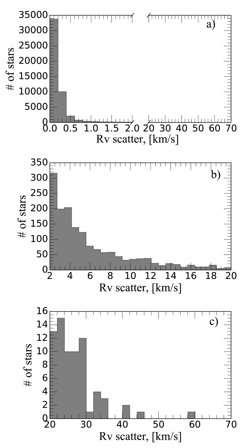
Figure 1: Histograms of the RV scatter of the selected APOGEE Milky Way disc subgiants and giants in DR12. a) Full distribution of the RV scatter. b) and c) Zooms of the tail of the RV scatter; note the change in the scale on the $y$-axes.

1 Introduction

Stellar multiplicity is a key parameter for many astrophysical questions. Several interesting astronomical phenomena, such as gravitational waves (Abbott et al., 2016), gamma-ray bursts (Murguia-Berthier et al., 2014) and certain types of supernovae (see Maoz et al., 2014, for a review) arise from binary stars. For ongoing and up-coming large spectroscopic surveys, such as RAVE (Kunder et al., 2017), APOGEE (Majewski et al., 2017a), Gaia-ESO (Gilmore et al., 2012), GALAH (De Silva et al., 2015), LAMOST (Deng et al., 2012), 4MOST (de Jong et al., 2016), MOONS (Cirasuolo & MOONS Consortium, 2016), and WEAVE (Dalton, 2016) it is important to identify as well as quantify the binaries in order to understand the underlying population and avoid the errors that can arise from mis-identifying binaries as single stars. The knowledge of multiplicity also provides constraints on possible channels of star formation and evolution in the Galaxy.

Surveys of binary stars suggest that the frequency of multiple systems is in the range of about 22 % to 80 %, where the binary fraction is higher for more massive stars (see Duchêne & Kraus, 2013, for a review). The most recent study of binary stars in the solar neighbourhood is by Raghavan et al. (2010). They updated and extended the sample of Duquennoy & Mayor (1991), combining several observational techniques to search for companions around 454 F6 – K3 type stars located within 25 pc of the Sun. They find that 54% $\pm$ 2% of solar-type ($\sim$F6–K3) stars in the solar neighbourhood are single, in contrast to the results of earlier multiplicity studies (Abt & Levy, 1976; Duquennoy & Mayor, 1991), who found 33% of solar-type (F3-G2) and 43% of G-dwarfs are single, respectively. Fuhrmann (2011) studied an unbiased, volume-complete sample of more than 300 nearby solar-type stars and showed that than 47% of stars are single, and that at least 15% belong to triple and higher order multiple systems.

Unresolved binaries can appear in spectroscopic observations in two different forms. If both stars are of similar brightness in the observed spectral region, lines from both stars will be visible. Such a binary is referred to as a double-lined spectroscopic binary (SB2). Unless the relative velocities of the two stars projected onto the line of sight are too similar or the spectral resolution is low, the Doppler shift owing to the relative motion of the two stars separates their spectral lines, so these binaries can be recognised from a single spectrum. For example, the Geneva-Copenhagen Survey (Nordström et al., 2004; Holmberg et al., 2009) identified 19% spectroscopic binaries in their $\sim$14 000 solar neighbourhood F-G type dwarf sample.

If, however, one of the components in a binary system is significantly fainter than the other its spectral features are not detected, and we have a single-lined spectroscopic binary (SB1). SB1s can typically only be identified via multiple observations. An example is the RAVE survey, in which 10% to 15% of stars with multiple observations are SB1 candidates (Matijevič et al., 2011). However, not all large-scale surveys have the repeated observations of stars that allow us to identify spectroscopic binaries.

Contamination by binaries has been shown to affect stellar parameters derived from spectra. In particular, for a low-resolution optical spectroscopic survey such as SEGUE, the temperature and metallicity of $\sim 10\%$ of stars will be noticeably affected by the presence of an undetected secondary (Schlesinger et al., 2010). For APOGEE-like spectra of solar-type stars El-Badry et al. (2018) find typical systematic errors of 300 K in $T_{\rm eff}$ and 0.1 dex in [Fe/H]. They show that binarity leads to larger systematics for near-infrared than for optical spectra because lower-mass companions contribute a larger fraction of the total light in the near infrared.

In this paper we present our model of the effect of binaries on high-resolution spectroscopic surveys, in order to determine how many binaries will be observed, whether unresolved binaries will contaminate measurements of chemical abundances, and how we can use spectroscopic surveys to better constrain the population of binaries in the Galaxy. As an application we model binary stars that mimic subgiants and giants observed by the Apache Point Observatory Galactic Evolution Experiment (APOGEE) in the Galactic disc. We use the APOGEE data included as part of the Sloan Digital Sky Survey’s 12th data release Alam et al. (2015).

Badenes et al. (2018) carried out an analysis of binaries in the APOGEE sample, based on the maximum radial velocity difference $\Delta RV_{\rm max}$ in the sample of radial velocities determined for an individual star. They show that the inferred binary fraction at the present day is a strong function of $\log g$, consistent with giants in close binaries being depleted by Roche lobe as they ascend the giant branch. They also report a strong metallicity dependence of the binary fraction. However, they do not model the details of stellar and binary evolution, which limits the extent to which they can connect the APOGEE giant population to the birth distributions of the binaries. Here we carry out such an analysis.

A brief outline of our paper is as follows. The sample of subgiants and giants selected from APOGEE is presented in Section 2. In Section 3 we describe the binary-evolution algorithm and our choices of initial parameters for the model binary population. In section 4 we present the synthesis of the APOGEE observation from models. Then we present our results of binary population models to examine the effects of binaries on high-resolution spectroscopic surveys in Section 5. Finally, we summarise our main results, draw conclusions and explore some perspectives in Section 6.

2 APOGEE subgiants and giants

APOGEE is a high-resolution ($R\approx 22\,500$), high signal-to-noise ($\approx$ 100/pixel) infrared (1.51–1.70 micron) spectroscopic survey. The target selection was defined using the Two Micron All Sky Survey Point Source Catalog (2MASS PSC) photometry (Skrutskie et al., 2006). Stars were selected from the 2MASS PSC employing de-reddened photometry with $H$ band magnitude $7\leq H\leq 13.2$. A simple colour cut of $(J-K_{S})_{0}\geq 0.5$ was made to include stars cool enough for a reliable derivation of stellar parameters and abundances, and to keep the fraction of nearby dwarf stars in the sample as low as possible. Close double or multiple sources are not resolved by 2MASS if their angular separation is $\leq 6^{\prime\prime}$ whereas the effective resolution of the 2MASS system is approximately $5^{\prime\prime}$ (Zasowski et al., 2013). APOGEE adopted data quality criteria for targets that the distance to nearest 2MASS source for $J$, $H$, and $K_{S}$ needs to be $\geq 6^{\prime\prime}$. The APOGEE fibres are $2^{\prime\prime}$ in diameter, so this exclusion radius means that no two separate 2MASS sources would be included on the same fibre.

Data release 12 (DR12 hereafter) was the final product of the third phase of the Sloan Digital Sky Survey (Eisenstein et al., 2011) and presented parameters for 146 000 stars. The APOGEE Stellar Parameters and Abundance Pipeline (ASPCAP; García Pérez et al., 2016) was used to derive $T_{\rm eff}$, $\log g$, [Fe/H], and elemental abundances by a $\chi^{2}$ minimisation of the differences between the observed spectra and a set of synthetic spectra. Holtzman et al. (2015) compare the temperatures, gravities, and metallicities with photometric temperatures, seismic gravities, and literature values for open and globular cluster members, respectively. They report random uncertainties of $\approx$ 100 K for Teff, 0.1 dex for $\log g$, and 0.05 dex for [Fe/H].

The radial velocities (RVs) for each observation are measured as part of the APOGEE data reduction pipeline (Nidever et al., 2015). Initial RVs are determined by cross-correlating the APOGEE spectra with a grid of synthetic spectra. Next, all the individual observations are shifted and co-added into a combined spectrum. This combined spectrum is then used as the template to re-derive the RVs of the individual epochs, again by cross-correlation. Nidever et al. (2015) found that for the red giants with 3 or more visits and total S/N per pixel $>20$ the mode of the rms RV scatter was 80 m/s. They conclude that this represents the random uncertainty in APOGEE’s RV measurements. Badenes et al. (2018) report a larger typical uncertainty of $0.2\,{\rm km\,s^{-1}}$. The interesting aspect of APOGEE for our work is that the majority of the stars have been observed multiple times. APOGEE began observations in May 2011 (Majewski et al., 2017b) and DR12 contains observations through July 2014 (Alam et al., 2015). This spread in observation times provides an RV time series which encodes enough information to detect companions to stars.

2.1 Star selection

Following the survey targeting strategy for different Galactic components we choose to look at subgiants and giants located in the Galactic disc, where 24^∘ $\leq$ $l$ $\leq$ 240^∘, $|b|$ $\leq$ 16^∘. We select stars for which:

1. stars.nvists > 2;

2. MIN(snr) > 20;

3. aspcap.aspcapflag & dbo.fApogeeAspcapFlag
   (“STAR$\_$BAD") = 0 and aspcap.teff > 0;

4. star.starflag & dbo.fApogeeStarFlag
   (“SUSPECT$\_$RV$\_$COMBINATION") = 0;

This selection finds stars that have been visited more than two times (1) as well where the individual stars’ spectra signal-to-noise ratio (S/N) is $\geq$ 20 (2). The next selection step finds a set of stars without any of the flags set that indicate that the observation’s RVs (3) or analysis of atmospheric parameters eg., T_eff (4) is bad.

To avoid contaminating our sample with stars that have their RV scatter inflated by badly-reduced spectra, we select stars using the flag “SUSPECT_RV_COMBINATION$=0$"; i.e. RVs from synthetic template will not differ significantly from those from combined spectrum. This has the additional effect of removing double-lined spectroscopic binaries (SB2s) from the sample since these have spectra which are morphologically different from spectra of single stars.

We select from this potential list of stars only the subgiants and giants (where $\log g\leq 4$) with effective temperatures in the range of $3500\,{\rm K}\leq T{{}_{\rm eff}}\leq 5500\,{\rm K}$. In DR 12 stars have a cutoff temperature of 3500 K on the cool side of the spectral grid. We choose to cut on stellar parameters rather than photometry since that gives a more reliable comparison between the models and data.

In order to constrain the Galactic binary population from our model we wish to model the RV variability of stars that mimic the APOGEE sample and test whether the observed scatter is comparable with variations induced by binaries. We quantify this as the RV scatter, $\sigma_{\rm RV}$, defined as the standard deviation of RV measurements for stars in the sample with multiple visits. Hence our final cut is to retain only stars with three or more RV observations. This leaves us with a final sample of 49731 stars. In Figure 1 we show histograms of the RV scatter of the selected stars. The scatter comes from several sources: for example, instrumental calibration errors, finite telescope resolution, and binary stars. We discuss this further in Section 5.2.

3 Binary star evolution models

3.1 Binary star evolution algorithm (bse)

Our modelling of single and binary star evolution is performed using the rapid binary-star evolution algorithm bse, presented in Hurley et al. (2002). bse enables us to model the evolution of binary systems containing stars of arbitrary initial mass, metallicity, orbital separation, and eccentricity. In addition to all aspects of single-star evolution, bse includes mass transfer and accretion from winds and Roche-lobe overflow, common-envelope evolution, merger, supernova kicks and angular momentum loss mechanisms. Orbit circularization and synchronisation by tidal interactions are included for convective, radiative and degenerate damping mechanisms.

bse is extremely fast, allowing us to model samples of tens of millions of binaries and hence obtain samples sufficiently large to compare to massive spectroscopic surveys. The cost of this is that bse is tied to the set of stellar evolution models that were used to construct it. We cannot, for example, incorporate models calculated with alpha abundances enhanced over scaled solar. However, this relatively minor limitation is compensated for by the ease with which we can compute the evolution of large populations of binaries.

bse contains a large number of tunable parameters. Many of these are not significant for our calculations – for example, the treatment of black-hole natal kicks does not affect our results since we observe vanishingly few binaries that contain black holes. For all parameters not described explicitly below we use the defaults as described in Hurley et al. (2002), a table of which can be found in Appendix A.

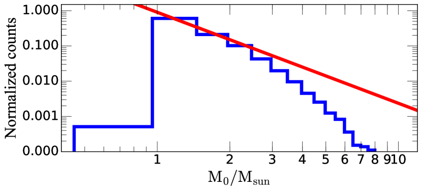
Figure 2: Histogram of the mass distribution for the primary stars in our sample of unresolved SB1 binaries. The red line shows the IMF for the initially most massive stars in our model.

3.2 Initial parameters for binary population evolution

In the following sections, we discuss the initial parameters used in our binary population synthesis, in particular our choice of mass distribution and orbital parameters. We distinguish between the initially most massive star, star 1 of mass $m_{1}$, and the primary, which is the most luminous star in the $H$ band at the time of observation. If star 1 has evolved – e.g. into a white dwarf – by the time of observation, then it may be seen as the secondary (less luminous star).

Table 1: Coefficients of the mass-generating function, Eq. (1).

$G_{1}$	$G_{2}$	$G_{3}$	$G_{4}$
0.19	1.55	0.05	0.60

3.2.1 Stellar masses

We assume that, for each binary, the initially more massive star has a mass between $0.9\,{\rm M}_{\odot}\leq m_{1}\leq 100\,{\rm M}_{\odot}$. We neglect stars with primary masses less than $0.9\,{\rm M}_{\odot}$ as they will not evolve into giants within the lifetime of the Universe. We generate $m_{1}$ from the initial mass function (IMF) of Kroupa et al. (1993), adopting their mass-generating function

$$m(x)=0.08+\frac{G_{1}x^{G_{2}}+G_{3}x^{G_{4}}}{(1-x)^{0.58}},$$ (1)

where $x$ follows a continuous uniform distribution on the interval $[0,1]$, $m(x)$ is in ${M_{\odot}}$, and the coefficients are given in Table 1. The mass of the companion is between $0.1\,{\rm M}_{\odot}\leq m_{2}\leq 100\,{M_{\odot}}$. The mass $m_{2}$ of the companion star is drawn assuming a mass ratio distribution

$$\rm{f(q)\propto q^{\gamma}},$$ (2)

where the mass ratio $q=m_{2}/m_{1}\leq 1$. In our standard model $\gamma$ = 0.0; i.e. the distribution is flat. Figure 2 shows the IMF for primary stars (red line) and the histogram of the final mass distribution of observed primary stars in a standard run. Above about $1\,{M_{\odot}}$ the distribution roughly follows the IMF, falling off more rapidly owing to the shorter lifetimes of more massive stars. Below about $1\,{M_{\odot}}$ most primaries have not evolved yet, and hence do not appear in our sample owing to the cut in $\log g$. There is a small contribution from stars below the turnoff mass that have accreted from a more massive companion.

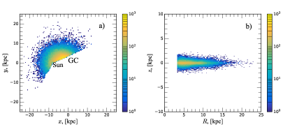
Figure 3: The positions of stars in the Galaxy generated in our model of the stellar disc. On the left: Galactocentric $x-y$ and on the right: $R-z$ plane. To mimic the APOGEE disc sample we only select stars in the model where Galactic longitude 24^∘ $\leq$ $l$ $\leq$ 240^∘ and Galactic latitude $|b|$ $\leq$ 16^∘. The colour coding indicate the number density of stars per bin (as shown in the colour bars).

3.2.2 Orbital properties of binary systems

We assign to each binary pair an initial orbital period in days, $P$, which follows a Gaussian distribution:

$$f(\log P)\propto\exp\Bigg{\{}{{\frac{-{(\log P-\overline{\log P})^{2}}}{2\sigma^{2}_{\log P}}}}\Bigg{\}}.$$ (3)

Here $\overline{\log P}$ = 4.8, equivalent to a peak in the distribution at $173\,{\rm yrs}$, and $\sigma$_logP = 2.3. A similar distribution is found by Raghavan et al. (2010) with $\overline{\log P}$ = 5.03 (293 years) and $\sigma$_logP = 2.28.

We allow our binary systems to form with eccentric orbits. The distribution of the orbital eccentricity, $e$, is chosen to be dynamically relaxed; i.e. binaries have all interacted with each other and exchanged energy many times and have reached statistical equilibrium. This thermal distribution thus follows (Heggie, 1975):

$$f(e)\varpropto 2e.$$ (4)

Each binary is assigned a random orientation with respect to the plane of the sky. In practice this is achieved by taking the longitudes of pericentre and ascending node to be uniform in $[0,2\uppi]$, and choosing the inclination $i$ so that $\cos i$ is uniform in $[0,1]$. The mean anomaly is taken to be uniform in $[0,2\uppi]$: i.e. the fraction of the orbital period that has elapsed since the last pericentre passage is randomly distributed at the present day. These four quantities, together with the stellar masses, orbital period and eccentricity, determine the initial position and velocity of the two stars. We convert to a Cartesian reference frame using a routine taken from mercury (Chambers, 1999). The angular separation measured at each observation is then calculated using the total separation in the $X-Y$ plane. The RV is taken to be the value along the $Z$ direction.

3.2.3 Ages and metallicities

Since stars in the Galactic disc have a broad age distribution, for our standard model we assign the age of the binary systems as uniformly distributed from 0 to 10 Gyr. As described below, we also test the effect of changing the age distribution.

bse was constructed by fitting functions to models at a fixed set of input metallicities. For metallicities between the input values bse interpolates the parameters in the fitting functions. This leads to significant errors in the morphology of the giant branch in the interpolated models. To avoid this problem we divide the APOGEE observations into bins centred on the bse input model metallicity values. The binning scheme is summarised in Table 2. Most solar-type stars in the Galactic field are near solar-metallicity; hence initially we consider the solar metallicity bin.

Table 2: Metallicity binning scheme.

	[Fe/H]		Number
min	model	max	of stars
-0.5	-0.30	-0.15	19243
-0.15	0.00	0.088	18221
0.088	0.17	0.45	9970

3.2.4 Description of our models with different initial conditions

To model the effects of binaries on high-resolution spectroscopic surveys, we must have a good understanding of their initial parameters. The initial binary parameters are uncertain because of limitations in the different techniques used to discern them (e.g., difficulties in the observations of the companion star; incorrect determination of masses because of rotation). However their properties, e.g. primary mass, mass ratio, orbital period, eccentricity, age, and metallicity, are beginning to be accurately quantified (Moe & Di Stefano, 2017). To test the influence of initial conditions on the final result we construct a variety of models, each with differing but reasonable assumptions for the initial parameters of the binary population. Table 3 lists the models and the parameters we choose to change from the standard setup. For all the models we synthesise a sample of $N=2\times 10^{5}$ binary stars.

Table 3: Distributions from which the binary properties are drawn in different model sets.

Model	$m_{1}$	$m_{2}$	$P$	$e$	${{\rm Age,~{}Gyr}}\atop{{\rm[min;~{}max]}}$
standard	KTG93a	$\gamma=0^{b}$	DM91c	te	$0:10$
m2FromIMF	KTG93	KTG93	DM91	t	$0:10$
qGamma0.3	KTG93	$\gamma=0.3$	DM91	t	$0:10$
qGamma1.0	KTG93	$\gamma=1$	DM91	t	$0:10$
periodR10	KTG93	$\gamma=0$	R10d	t	$0:10$
flatEcc	KTG93	$\gamma=0$	DM91	ff	$0:10$
old	KTG93	$\gamma=0$	DM91	t	$10:12$
young	KTG93	$\gamma=0$	DM91	t	$0:4$

Notes: [Fe/H]=0 for all the models given here; see Section 5.3. ^a KTG93: Mass is drawn from the initial mass function (IMF) from Kroupa et al. (1993). ^b Where $\gamma$ is given the mass ratio is selected using Equation 4. ^c DM91: Period distribution from Duquennoy & Mayor (1991). ^d R10: Period distribution from Raghavan et al. (2010). ^e t: thermal eccentricity distribution. ^f f: flat eccentricity distribution.

Our baseline model, standard, adopts the stellar population properties of described in Duquennoy & Mayor (1991). In m2FromIMF we assume that the secondary star masses, $m_{2}$, are drawn independently from the same the initial mass function as the primary, i.e. following Kroupa et al. (1993). Models qGamma0.3 and qGamma1.0 are generated with the mass ratio distribution following Eq. 2 with ${\gamma}=0.3$ and ${\gamma}=1.0$ respectively. In model periodR10 we choose the period distribution following Raghavan et al. (2010). The model flatEcc has the period distribution from Duquennoy & Mayor (1991) with a flat eccentricity distribution. In the two final models we check the effects of age. In one model (old) the age of our binary population is exclusively old (from 10 to 12 Gyr). In the other one (young) we generate a purely young population with binary systems uniformly distributed from 0 to 4 Gyr.

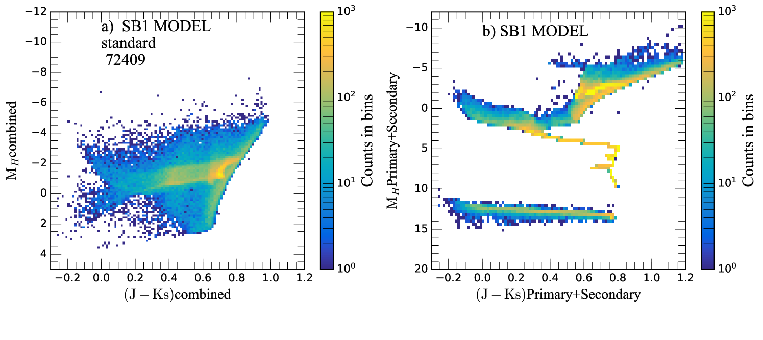
Figure 4: The theoretical colour-magnitude diagrams (CMDs) for single-lined binary stars (SB1s) in the standard model. a) The CMD for unresolved binaries, where the magnitudes and colours show the combined light of both stars. b) the same binaries are shown but magnitudes and colours for primaries and secondaries are plotted separately; the low mass main-sequence stars and white dwarfs that appear are secondaries.

We checked the effects of metallicity on the evolving binary star population by running models with [Fe/H] = [$-$0.30; 0.0; 0.17]; see Section 5.3 for further discussion.

3.3 Galaxy model

To correctly determine the selection of stars we need to know how far away from the Sun they are. We distribute the stars according to a model of the Galactic disc. We take the disc to be an exponential with radial scale length $h_{R}=3.0\,{\rm kpc}$ and vertical scale height $h_{z}=0.3\,{\rm kpc}$ (Rix & Bovy, 2013). In this model the Sun is located 8 kpc from the centre of the Galaxy. We only include the thin disc stars since the APOGEE sample is in the Galactic plane which is dominated by the thin disc. To mimic the APOGEE disc sample we only select stars with 24^∘ $\leq$ $l$ $\leq$ 240^∘ and $|b|$ $\leq$ 16^∘ (see Fig. 3).

4 Synthetic APOGEE observations

We evolve the binary population using bse. bse calculates the stellar luminosity $L$, radius $R$, mass $M$ etc. for both stars in the binary system as they evolve. In order to mimic the APOGEE observations and to calculate relative line-of-sight velocities we make multiple synthetic observations of each model binary. First, we create an observing schedule for each binary by randomly selecting one of the actual observing schedules from APOGEE DR 12. At each observation time we calculate the separation on the sky (in the $X-Y$ plane) and relative velocity along the line-of-sight (the $Z$ direction). Other than the effect of the varying orbital phase on the projected angular separation and RVs we keep the properties of the binary constant between the observations – this is reasonable given the long timescales of stellar evolution compared to the duration of APOGEE observations.

For a star with a given set of parameters (surface gravity, effective temperature, mass, radius, metallicity etc.) we calculate absolute $J$, $H$, $K_{S}$ magnitudes and $(J-K_{S})$ colours in the 2MASS system using bolometric corrections from Marigo et al. (2008).

To mimic the APOGEE observations we need to work out how APOGEE would observe each of our model systems. A resolved binary star is defined as one where the two components can be resolved into individual stars. In this study we define a resolved binary as one where the two stars are separated on the sky by 6^′′ or more; see Section 2. We analyse such binaries as two separate stars. To mimic the selection process for APOGEE we require that the combined magnitude for a unresolved binary is not too faint ($M_{H}\leq 13.2$) (Zasowski et al., 2013).

We define a single-lined spectroscopic binary, SB1, as a binary pair where the flux ratio of the two components as measured in H-band is $\geq 10$. A double-lined spectroscopic binary, SB2, is defined as a binary system where this flux ratio is $0.1\leq F_{\rm ratio}\leq 10$.

Since we are concerned with modelling the red giant stars from APOGEE DR12 we have chosen to limit our model sample to binary systems where the primary component has $\log g\leq 4$. It is straightforward to change this constraint to suit the observations that are being investigated.

5 Results

In this section we first present the results of our model in general terms, then make a quantitative comparison with the APOGEE data to constrain the multiplicity frequency. As we have removed double-lined binaries (SB2s) from the data (see 2.1) we consider only the SB1 portion of the model here.

5.1 Observed vs. simulated population properties

Synthesised colour-magnitude diagrams (CMDs) of single-lined binaries (SB1) from the standard run are shown in Figure 4. The CMD for unresolved binary stars is shown in panel a). The absolute magnitude is calculated based on the combined flux of the two stars in the system. The observed CMD is dominated by red giant branch (RGB) and red clump (RC) stars, consistent with our selection criteria. In panel b) we show the same population of binaries but plot the absolute magnitudes and colours for the primaries and secondaries separately. The majority of the secondaries are faint white dwarfs or low-mass main-sequence stars.

The percentage of different stellar types in the standard run is illustrated in Fig. 5. The binaries mostly comprise RC primaries with MS secondaries ($\approx\,50\%$) and RGB primaries with MS secondaries ($\approx\,27\%$). A smaller proportion ($\approx\,17\%$) of these giant primaries have compact object (CO) secondaries. There are also small populations of asymptotic giant branch (AGB) ($\sim\,2\%$) and Hertzsprung Gap (HRGap) stars ($\sim\,1\%$) as primaries with MS secondaries.

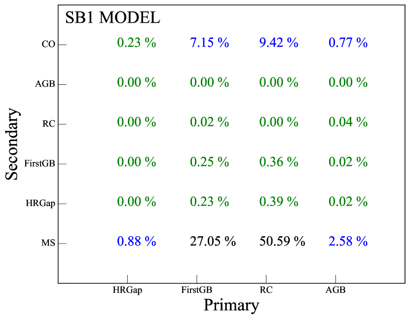
Figure 5: Stellar types of model binaries observed as single-lined spectroscopic binaries (SB1) in the standard run. The abscissa shows the type of the primary (brighter) star and the ordinate the type of the secondary (fainter) star. The bulk of binaries have their primary star on the first giant branch or red clump, with the companions mostly being main-sequence stars.

As a first, qualitative comparison between our model and the observed RV scatter in the APOGEE data we plot the velocity scatter, $\sigma_{\rm RV}$, versus stellar parameters $T_{\rm eff,Primary}$ and $\log(g)_{\rm Primary}$ (Figure 6). The qualitative agreement between simulated and observed results is good. In both model and observations the velocity scatter decreases as the stars become more evolved: i.e. as $T_{\rm eff}$ and $\log(g)$ decrease. This is expected, since the star that we observe is the more evolved, cooler primary. As stars evolve their radii increase. Therefore, binary orbits in which giants can exist must be on average larger than the orbits of dwarfs: hence the orbital periods are longer and consequently the binary-induced RV scatter is lower. The same trend was reported by Badenes et al. (2018) in the analysis of the APOGEE observations. The plots are for the standard model but similar qualitative behaviour is also seen when the input distributions are varied.

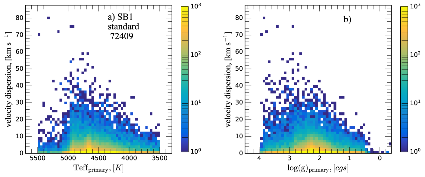
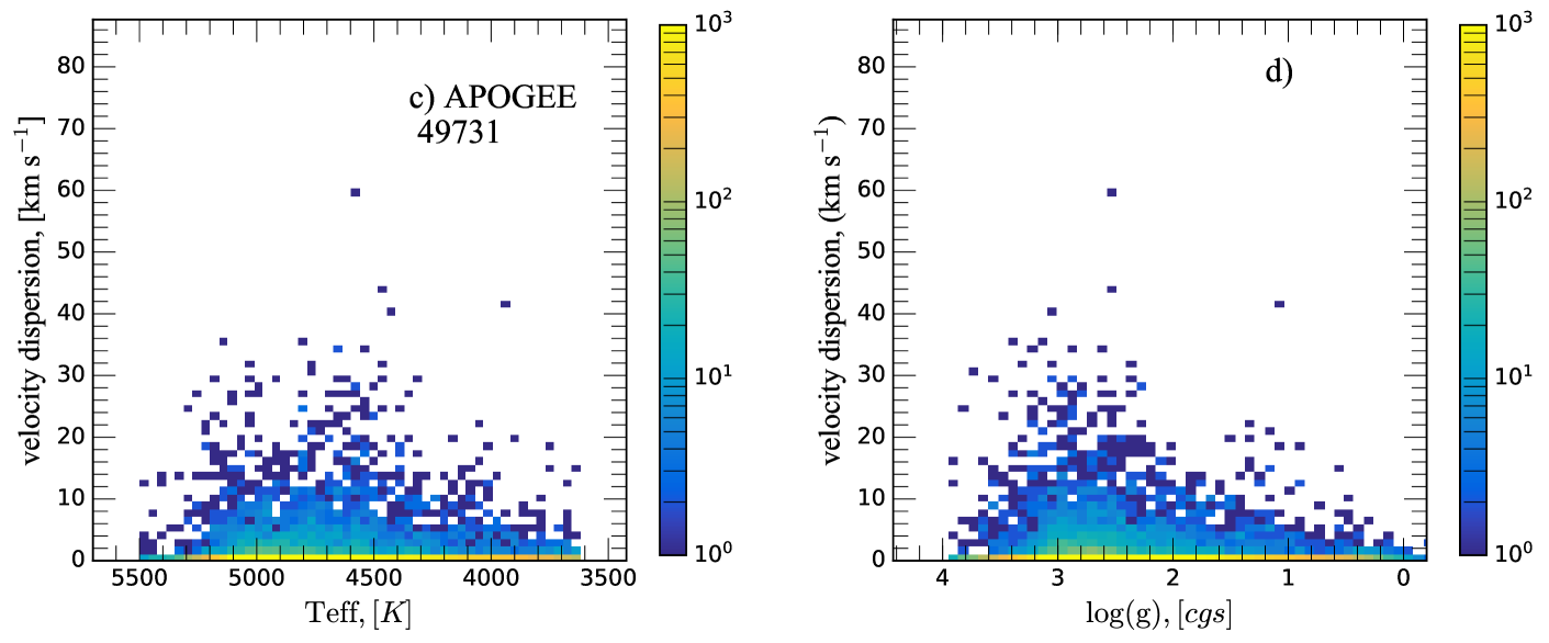
Figure 6: Velocity scatter versus atmospheric parameters $T_{\rm eff,Primary}$ and $\log(g)_{\rm Primary}$ from a) and b) the SB1 model, and c), d) APOGEE DR 12. The colour coding indicates the number density of stars.

5.2 Multiplicity frequency in the field

Our model allows us to estimate the binary fraction in the Milky Way fields observed by APOGEE. We do this by fitting $F\left(\sigma_{\rm RV}\right)$, the cumulative distribution of the standard deviation of observed RVs in the APOGEE sample. We expect that this relationship could vary with metallicity even though we use the same distributions of birth properties such as mass ratio. For example, the range of possible orbital velocities in a binary is determined by the relationship between stellar masses and radii, which differs with metallicity. For the same reasons the relationship in our models between the initial binary fraction $f_{\rm b,0}$ and the observed binary fraction at the present day varies with metallicity. Hence we split the APOGEE sample up by metallicity. We choose bins centred on the metallicity values for which the stellar evolution models that underlie bse were constructed, since the giant branch models that it produces are most reliable at those metallicity values (see Section 3.2.3). Our binning scheme is given in Table 2.

The RV variations of the stars in the APOGEE sample come from many sources. Some are astrophysical: for example, binaries and higher order stellar multiple systems, star spots, oscillations of the stellar surfaces, and planetary systems. Some are not: for example, errors in instrumental calibration and data reduction. We lump together all the RV variations not caused by binaries and model them with a single distribution. In practice we find that this distribution is adequately described by a log-normal distribution whose mean $\mu_{s}$ and standard deviation $\sigma_{s}$ become nuisance parameters to be fit. The RV variations from binaries we obtain separately from our model.

In detail, we synthesise a mixed sample of single stars and binaries. At birth, a fraction $f_{\rm b,0}$ of our objects are binaries, the remaining $1-f_{\rm b,0}$ being single stars. In this definition the initial binary fraction is

$$f_{\rm b,0}\equiv\left.\frac{N_{\rm binaries}}{N_{\rm single}+N_{\rm binaries}}\right|_{\rm birth}.$$ (5)

For each star or binary that we generate we draw from the appropriate synthesised sample described in Section 4. If it does not meet the selection criteria described in Section 2, for example because it is too faint, we discard it. Otherwise we make a synthetic observation as follows. We first obtain an observing schedule by drawing randomly from the APOGEE visit schedule. For each visit we draw a velocity from the log-normal distribution characterised by $\sigma_{s}$ and $\mu_{s}$ to produce a synthetic set of RVs. In addition, for binaries, we obtain from our model the velocity owing to the primary star’s motion around the binary’s barycentre, projected onto the line of sight at the visit times, and add them to the values from the log-normal distribution. Finally we take the standard deviation to measure the scatter. This process is continued until we have made synthetic observations of the same total number of objects as in our APOGEE sample. We then sort by scatter to obtain the cumulative distribution of RV scatter in the model, which we denote $F_{\rm mod}(\sigma_{\rm RV})$.

Having done this we calculate a goodness-of-fit parameter $Q$ from the cumulative distributions of scatter in the APOGEE data, $F_{\rm obs}(\sigma_{\rm RV})$, and in the model $F_{\rm mod}(\sigma_{\rm RV})$, as

$$Q=\int_{0.01\,{\rm km\,s^{-1}}}^{20\,{\rm km\,s^{-1}}}\left(\log F_{\rm obs}-\log F_{\rm mod}\right)^{2}{\rm d}\log\sigma_{\rm RV},$$ (6)

where the cumulative fraction runs from high velocities to low velocities. This form for $Q$ is chosen to emphasise the high-scatter objects (i.e. the binaries) at the expense of the low-scatter (i.e. single) stars. The limits of the integral are chosen to exclude a handful of outliers that make the measurement noisy. Using this definition for $Q$ we find a best-fit model by minimising $Q$ with respect to the model parameters $f_{\rm b,0}$, $\mu_{s}$ and $\sigma_{s}$. For small values of $Q$ (well-fitting models) the value is dominated by random scatter; in these cases we calculate 200 realisations of our model with the same parameters and choose the median value of $Q$. The results are shown in Figure 7. The model including both binary and single stars reproduces the main features and shape of the distribution well. This suggests that the major cause of high-amplitude velocity scatter in the APOGEE sample is indeed the presence of binary stars.

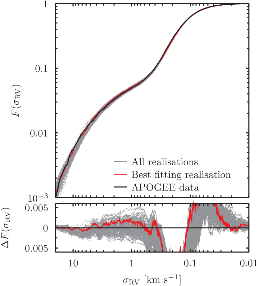
Figure 7: Top panel: Cumulative radial velocity scatter distributions $F(\sigma_{\rm RV})$ for the best-fitting model. The black line shows the APOGEE data in the bin around solar metallicity. The grey lines show 200 realisations of the model with the best fitting parameters ($f_{\rm b,0}=0.35$, $\mu_{s}=-0.71$ and $\sigma_{s}=0.29$). The best fitting of the 200 realisations is shown in red. Bottom panel: The same data plotted as as the difference between the model and observational data. The relatively poor fit at low RVs ($\sigma_{\rm RV}\lesssim 0.5\,{\rm km\,s^{-1}}$) is because the intrinsic scatter is not exactly fit by a single log-normal distribution.

Having derived the best fit values we apply the technique of approximate Bayesian computation as presented by Turner & Zandt (2012). We assume flat priors on all three parameters and calculate $Q$ for a grid of models that span the best-fit values. Realisations of the model that have $Q$ less than a critical value $Q_{\rm crit}$ then sample the posterior distributions of our parameters directly. We find that the process has converged at $Q_{\rm crit}\approx 0.02$. Plots of the inferred one-dimensional posterior probability distributions of the parameters and two-dimensional covariance distributions for the bin centred on solar metallicity are shown in Figure 8. Once we have marginalised over the nuisance parameters $\mu_{s}$ and $\sigma_{s}$ we find that the posterior probability distribution of the initial binary fraction $f_{\rm b,0}$ is well described by a Gaussian, and that for solar metallicity $f_{\rm b,0}=0.35\pm 0.01$.

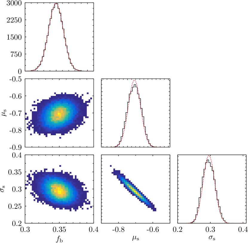
Figure 8: Marginalised posterior probability density distributions for the parameters of our model fit. The parameters are the binary fraction at birth, $f_{\rm b,0}$, and the mean and standard distribution of the RV scatter intrinsic to the observations, $\mu_{s}$ and $\sigma_{s}$. The red dashed lines represent Gaussian fits to the one-dimensional distributions. The calculations were carried out for the metallicity bin centred on solar metallicity; see Section 5.2 for details.

5.3 Variation of binary fraction with metallicity

We repeat the above analysis for the metallicity bins immediately above and below Solar metallicity. The results for all three bins are shown in Table 4. We reproduce the declining trend in binary fraction with metallicity found by other authors in the APOGEE sample (Badenes et al., 2018) and in other samples such as LAMOST or SEGUE (Yuan et al., 2015; Gao et al., 2017). The binary fractions deduced from the LAMOST and SEGUE samples are consistent with our results within the uncertainties. Both samples show the same trend: the fraction of binaries is smaller for stars of redder colours and higher metallicities. On the other hand Hettinger et al. (2015) found that, for F-type stars in the Milky Way, metal-rich stars were 30% more likely to have companions with periods shorter than 12 days than metal-poor stars. Our sample is dominated by red clump and RGB stars, which, by the time APOGEE observes them, have evolved to be too large to fit in such a close binary. Hence the binaries discussed by Hettinger et al. (2015) would not be present in our sample or in our model output since they would have interacted before either star reached the giant branch.

Table 4: Effect of metallicity on the inferred initial binary fractions.

[Fe/H]	$f_{\rm b,0}$	$\mu_{s}$	$\sigma_{s}$
-0.30	$0.37\pm 0.01$	$-0.64\pm 0.05$	$0.31\pm 0.02$
0.00	$0.35\pm 0.01$	$-0.71\pm 0.04$	$0.29\pm 0.02$
0.17	$0.30\pm 0.01$	$-0.74\pm 0.05$	$0.29\pm 0.03$

5.4 The effect of initial conditions

Table 5: Effect of binary initial conditions on inferred binary fraction at Solar metallicity

Model set	$f_{\rm b,0}$	$\mu_{s}$	$\sigma_{s}$	Odds
				ratio
standard	$0.35\pm 0.01$	$-0.71\pm 0.04$	$0.29\pm 0.02$	1.0
m2fromIMF		No good fit		$<10^{-3}$
qGamma0.3	$0.34\pm 0.01$	$-0.72\pm 0.04$	$0.30\pm 0.02$	1.8
qGamma1.0	$0.32\pm 0.01$	$-0.73\pm 0.03$	$0.31\pm 0.01$	3.5
periodR10	$0.37\pm 0.01$	$-0.70\pm 0.04$	$0.29\pm 0.02$	0.38
flatEcc	$0.33\pm 0.01$	$-0.70\pm 0.04$	$0.29\pm 0.02$	0.33
old	$0.32\pm 0.01$	$-0.72\pm 0.03$	$0.30\pm 0.01$	2.0
young	$0.12\pm 0.01$	$-0.71\pm 0.03$	$0.30\pm 0.01$	1.2

We repeat the analysis from Section 5.2 for the different set of binary properties given in Table 3; see Table 5 for the results. Good fits are obtained for all models other than the m2FromIMF model, in which we draw the masses of both stars independently from the IMF. The values of $\mu_{s}$ and $\sigma_{s}$ are independent of the binary model used within the uncertainties. This is expected, since they are properties that primarily affect the single stars where they are the only source of observable velocity scatter, and hence their constancy is a necessary condition for the models to be good fits. The values of $f_{\rm b,0}$ do, however, change depending on the model used. This is because different sets of assumptions about the binary properties lead to different fractions of binaries evolving into the range of parameter space where they contribute to the scatter in APOGEE observations. The final column shows the odds ratio, calculated as the fraction of the three-dimensional phase space contributing systems to the posterior distribution at a given cut in $Q$, relative to the standard model set. Were the different sets of initial conditions equally likely a priori this could be interpreted as their relative likelihood, and hence gives an indication of how strongly the different possibilities are supported by the data.

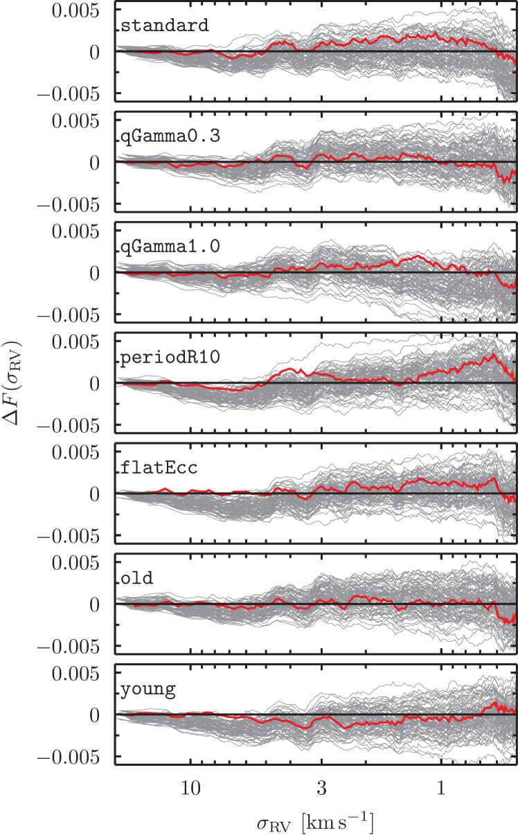
Figure 9: Difference between the cumulative distribution of the APOGEE observations and that of the model, $\Delta F(\sigma_{\rm RV})=F_{\rm mod}(\sigma_{\rm RV})-F_{\rm obs}(\sigma_{\rm RV})$, as a function of the RV scatter $\sigma_{\rm RV}$. Each panel shows a different set of initial conditions as given in Table 3. The grey lines show 100 realisations of the model, each with the best-fit parameters taken from Table 5, and the red line shows the best fitting of these models for each parameter set. The black line shows the offset for the data, which is zero by definition. Only the part of the plot up to $0.5\,{\rm km\,s^{-1}}$ is shown since the lower velocities are dominated by single stars and binaries with negligible reflex motion. The distribution for the m2fromIMF initial conditions is omitted since no good fit was found.

In Figure 9 we plot the differences between the observed and model cumulative scatter distributions, $\Delta F(\sigma_{\rm RV})$, for the different models. For each set of binary parameters we show 100 realisations of the best fit model given in Table 5, with the best fitting of those 100 highlighted in red. Each of the models shows rather similar behaviour, and changing the input parameters within these reasonable bounds of disagreement shows no significant improvement to the fit. The only exception is the model where we draw both stars independently from the IMF, which is very strongly disfavoured. This implies that the binaries that we are able to constrain using this model come from a limited sub-set of the initial binary populations, a hypothesis that we now go on to test.

5.5 Which binaries does the APOGEE data constrain?

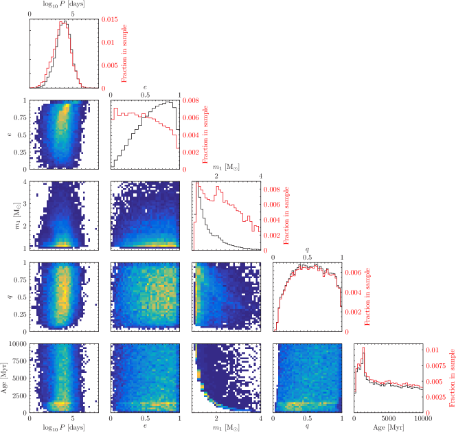
Figure 10: Distributions of birth properties of the binaries in our model which we predict would be found in APOGEE with a projected RV scatter $\sigma_{\rm RV}>0.5\,{\rm km\,s^{-1}}$. The quantities plotted, left to right along the abscissa, are: the log of the binary period in days; the eccentricity; the mass of the initially most massive star, $m_{1}$, in ${M_{\odot}}$; the mass ratio $q$; and the age in Myr. The colour maps show two-parameter correlations. The top panel in each column shows the distribution of that property in the sample. The black line shows the relative number of stars at different property values that meet the selection criteria and have $\sigma_{\rm RV}>0.5\,{\rm km\,s^{-1}}$. The red line (with labels on the right-hand axis) shows the fraction of the complete initial sample of binaries that meet our selection criteria to be observed by APOGEE and have $\sigma_{\rm RV}>0.5\,{\rm km\,s^{-1}}$. Where this has a different shape to the black line it is because the distribution of stars in the initial sample is significantly non-uniform across the relevant parameter range (e.g. for the eccentricity).

Figure 10 shows the birth properties of binaries in our sample of synthetic APOGEE observations that have $\sigma_{\rm RV}>0.5\,{\rm km\,s^{-1}}$. This value was chosen as the approximate point where the cumulative distribution goes from being dominated by non-binary RV scatter to RV scatter produced by the binary orbit. Hence these are the binaries that our analysis is sensitive to. Binaries with other initial properties also appear in our sample, but have insufficient velocity scatter to be clearly separated from single stars. Roughly half of the binaries in our synthetic observations lie above this limit; binaries below this limit cannot be detected through RV scatter alone.

Figure 10 shows that the main quantity that determines whether a binary is observed to have $\sigma_{\rm RV}>0.5\,{\rm km\,s^{-1}}$ is the initial period. The binaries that appear mostly have periods between $10^{3}$ and $10^{4}$ days. They are thus sufficiently wide that neither star has filled its Roche lobe before becoming a giant, but close enough that they still have a sufficiently high RV that $\sigma_{\rm RV}>0.5\,{\rm km\,s^{-1}}$. Appearance is largely independent of initial eccentricity, except at very high eccentricity where the separation at pericentre is greatly reduced. The visible correlation between the mass of the initially most massive star, $m_{1}$, and age is because, for the most massive star to appear in the APOGEE sample, it must have evolved to the giant branch but no further. The other effect that is visible is a weak preference for young ages. This may be because the stars that are evolving on to the giant branch at these ages never develop degenerate cores, and hence never grow as large on the first giant branch. Hence a larger range of orbits can survive to the horizontal branch, where the star is longer-lived in the APOGEE-observable sample.

These effects explain the differences in binary fractions seen in Table 5. At young ages there are a higher fraction of binaries visible in the model, so the young sample requires a smaller binary fraction to reproduce the observed scatter. The Raghavan et al. (2010) distribution has a smaller fraction of binaries in the period range where they influence our model so a slightly larger binary fraction is required. The other binary properties have little effect on the population of binaries with $\sigma_{\rm RV}>0.5\,{\rm km\,s^{-1}}$ and hence do not change the binary fraction that we infer.

6 Conclusions and discussion

We have synthesised realistic stellar populations, composed of a mix of single and binary stars, using the rapid binary-star evolution code bse. As an application we model the effect of binary stars on observations of Galactic disc stars in the Apache Point Observatory Galactic Evolution Experiment (APOGEE DR 12). We compare the radial velocity (RV) scatter in representative samples at different metallicities and find that the scatter found at velocities above $0.5\,{\rm km\,s^{-1}}$ in the APOGEE data is adequately reproduced by the effects of stellar binaries. We find correlations between the stellar atmospheric parameters and RV scatter that are similar to those in the APOGEE sample. The APOGEE sample is sensitive to the full range of binary eccentricities and mass ratios, primary star masses between the turnoff mass and a few solar masses, and initial binary periods between 3 and 3000 years.

Using this approach we constrain the birth binary fraction of solar metallicity binaries to be $f_{\rm b,0}=0.35\pm 0.01$. This is consistent with the study of solar-neighbourhood, solar-type binaries by Raghavan et al. (2010), who find $f_{\rm b,0}=0.33\pm 0.02$. Our results are relatively insensitive to reasonable choices of initial binary properties. Both the period distributions of Raghavan et al. (2010) and Duquennoy & Mayor (1991) are consistent with the data, with a slight preference for the latter. Similarly flat and thermal eccentricity distributions both lead to good fits, with a slight preference for a thermal distribution. The mass ratio distribution is somewhat better fit with a mild bias towards equal mass ratios; a power-law with index $\gamma=1$ fits better than a flat distribution, and choosing both stars independently from the IMF is ruled out. We are largely insensitive to the stellar age distribution. The majority of stars observed by APOGEE are old, and hence significant changes in the age distribution only translate to small changes in the distribution of initial stellar masses in the observed sample. Hence assuming a flat age distribution with a broad range of ages is sufficient.

An extension of this work would be to fit the properties of the initial binary population simultaneously with the binary fraction. Whilst such an analysis would be possible, we have not attempted it here for two reasons. First, it would require either synthesis of a new sample for each model value explored, or synthesis of a much larger population of binaries which could then be re-sampled. Either option would be much more computationally intensive. Secondly, many of the properties of the population – e.g. the width of the distribution of orbital periods – are poorly constrained by our data and hence little would be gained by fitting for them. Instead of fitting for these parameters we have chosen to explore a range of reasonable values. The downside of this approach is that the uncertainties that we present in Table 5 are underestimates. A better estimate of the uncertainty on our measurement of the initial binary fraction can be seen in the scatter between different reasonable choices of initial conditions, which is of the order of a few percentage points.

We also study the effect of metallicity, and reproduce the trend of a declining binary fraction with increasing metallicity. This is in qualitative agreement with the hydrodynamic star-formation models of Machida et al. (2009), whose results indicate a higher binary frequency in lower metallicity gas. On the contrary, the recent results obtained from radiation hydrodynamical simulations by Bate (2014) suggest that stellar binaries are formed mainly by gravitational collapse, which is highly insensitive to the dust content of the protostellar disk. More comprehensive studies, particularly of large samples of dwarf stars where we are more sensitive to shorter-period binaries, are necessary to resolve this question.

We do not consider the lowest metallicity stars present in the APOGEE sample (i.e. those with [Fe/H]$<-0.5$). The reasons for this are two-fold. First, relatively few stars meet our criteria for inclusion, so the constraints available on the binary population are weaker. Secondly, we start to see an increasing population of sub-luminous, cold stars with high velocity dispersions in the APOGEE data, similar in appearance to Algols. Very few such stars are present at solar metallicity, but at lower metallicities they become quite common, a trend that is not well reproduced by our bse models. We leave investigation of these binaries to a subsequent study.

It is unsurprising that the binary reflex motion dominates the RV scatter at higher velocities. Other astrophysical sources of RV scatter include higher-order stellar multiples, planetary systems, stellar surface oscillations and varying star-spot cover. There is also scatter induced from errors in spectral analysis and instrumental effects. All of these contributions are expected to be smaller than the binary contribution, and this fits with the detailed predictions of our models. Therefore, although we are not sensitive to all binaries, we find that stellar surveys with multiple observations per star are sensitive to the overall binary population. Whilst we have focussed on giants in this paper, samples involving dwarfs will be sensitive to closer binaries, which do not in general form binaries as the stars interact before the reach the giant branch. We intend to investigate the local APOGEE dwarf sample in a follow-up paper.

Our analysis is easily adapted to other surveys with different observation schedules, selection functions, wavebands, etc. Careful consideration of the binary population is necessary to quantify the effects of unresolved binary systems on measurements derived from stellar spectroscopy. An analysis such as this one is useful to allow the effects of binaries on the survey science to be quantified and the survey design optimised to reduce the effects of binaries. We plan to expand a similar analysis to other existing spectroscopic surveys, large and small, and also surveys currently in planning and development such as WEAVE and 4MOST.

Appendix A Additional Data

The binary evolution algorithm described by Hurley et al. (2002) has a large number of tunable parameters. In Table 6 we list the values of the input parameters not described in more detail in Section 3.

Table 6: Input parameters for binary evolution in the bse algorithm.

Parameter	Value	Meaning
$\eta$	0.5	Reimers mass-loss coefficient
$B_{W}$	0.0	Binary enhanced mass loss parameter
$He_{W}$	1.0	Helium star mass loss factor
$\alpha_{CE}$	3.0	Common-envelope efficiency parameter
$\lambda$	0.5	Binding energy factor for common envelope evolution
$\sigma_{k}$	190	Dispersion in the Maxwellian for the SN kick speed (in km/s)
$\beta_{W}$	0.125	Wind velocity factor
$\upmu_{W}$	1.0	Wind accretion efficiency factor
$\alpha_{W}$	1.5	Bondi-Hoyle wind accretion factor
$\upepsilon$	0.001	Fraction of accreted matter retained in nova eruption
Eddfac	1.0	Eddington limit factor for mass transfer
$\Gamma$	-1.0	Angular momentum factor for mass lost during Roche lobe overflow

Note. The parameter values are the defaults, as described in Hurley et al. (2002).

References

- Abbott et al. (2016) Abbott B. P., et al., 2016, Physical Review Letters, 116, 061102
- Abt & Levy (1976) Abt H. A., Levy S. G., 1976, ApJS, 30, 273
- Alam et al. (2015) Alam S., et al., 2015, ApJS, 219, 12
- Badenes et al. (2018) Badenes C., et al., 2018, ApJ, 854, 147
- Bate (2014) Bate M. R., 2014, MNRAS, 442, 285
- Chambers (1999) Chambers J. E., 1999, MNRAS, 304, 793
- Cirasuolo & MOONS Consortium (2016) Cirasuolo M., MOONS Consortium 2016, in Skillen I., Balcells M., Trager S., eds, Astronomical Society of the Pacific Conference Series Vol. 507, Multi-Object Spectroscopy in the Next Decade: Big Questions, Large Surveys, and Wide Fields. p. 109
- Dalton (2016) Dalton G., 2016, in Skillen I., Balcells M., Trager S., eds, Astronomical Society of the Pacific Conference Series Vol. 507, Multi-Object Spectroscopy in the Next Decade: Big Questions, Large Surveys, and Wide Fields. p. 97
- De Silva et al. (2015) De Silva G. M., et al., 2015, MNRAS, 449, 2604
- Deng et al. (2012) Deng L.-C., et al., 2012, Research in Astronomy and Astrophysics, 12, 735
- Duchêne & Kraus (2013) Duchêne G., Kraus A., 2013, ARA&A, 51, 269
- Duquennoy & Mayor (1991) Duquennoy A., Mayor M., 1991, A&A, 248, 485
- Eisenstein et al. (2011) Eisenstein D. J., et al., 2011, AJ, 142, 72
- El-Badry et al. (2018) El-Badry K., Rix H.-W., Ting Y.-S., Weisz D. R., Bergemann M., Cargile P., Conroy C., Eilers A.-C., 2018, MNRAS, 473, 5043
- Fuhrmann (2011) Fuhrmann K., 2011, MNRAS, 414, 2893
- Gao et al. (2017) Gao S., Zhao H., Yang H., Gao R., 2017, MNRAS, 469, L68
- García Pérez et al. (2016) García Pérez A. E., et al., 2016, AJ, 151, 144
- Gilmore et al. (2012) Gilmore G., et al., 2012, The Messenger, 147, 25
- Heggie (1975) Heggie D. C., 1975, MNRAS, 173, 729
- Hettinger et al. (2015) Hettinger T., Badenes C., Strader J., Bickerton S. J., Beers T. C., 2015, ApJ, 806, L2
- Holmberg et al. (2009) Holmberg J., Nordström B., Andersen J., 2009, A&A, 501, 941
- Holtzman et al. (2015) Holtzman J. A., et al., 2015, AJ, 150, 148
- Hurley et al. (2002) Hurley J. R., Tout C. A., Pols O. R., 2002, MNRAS, 329, 897
- Kroupa et al. (1993) Kroupa P., Tout C. A., Gilmore G., 1993, MNRAS, 262, 545
- Kunder et al. (2017) Kunder A., et al., 2017, AJ, 153, 75
- Machida et al. (2009) Machida M. N., Omukai K., Matsumoto T., Inutsuka S.-I., 2009, MNRAS, 399, 1255
- Majewski et al. (2017a) Majewski S. R., et al., 2017a, AJ, 154, 94
- Majewski et al. (2017b) Majewski S. R., et al., 2017b, AJ, 154, 94
- Maoz et al. (2014) Maoz D., Mannucci F., Nelemans G., 2014, ARA&A, 52, 107
- Marigo et al. (2008) Marigo P., Girardi L., Bressan A., Groenewegen M. A. T., Silva L., Granato G. L., 2008, A&A, 482, 883
- Matijevič et al. (2011) Matijevič G., et al., 2011, AJ, 141, 200
- Moe & Di Stefano (2017) Moe M., Di Stefano R., 2017, ApJS, 230, 15
- Murguia-Berthier et al. (2014) Murguia-Berthier A., Montes G., Ramirez-Ruiz E., De Colle F., Lee W. H., 2014, ApJ, 788, L8
- Nidever et al. (2015) Nidever D. L., et al., 2015, AJ, 150, 173
- Nordström et al. (2004) Nordström B., et al., 2004, A&A, 418, 989
- Raghavan et al. (2010) Raghavan D., et al., 2010, ApJS, 190, 1
- Rix & Bovy (2013) Rix H.-W., Bovy J., 2013, A&ARv, 21, 61
- Schlesinger et al. (2010) Schlesinger K. J., Johnson J. A., Lee Y. S., Masseron T., Yanny B., Rockosi C. M., Gaudi B. S., Beers T. C., 2010, ApJ, 719, 996
- Skrutskie et al. (2006) Skrutskie M. F., et al., 2006, AJ, 131, 1163
- Turner & Zandt (2012) Turner B. M., Zandt T. V., 2012, Journal of Mathematical Psychology, 56, 69
- Yuan et al. (2015) Yuan H., Liu X., Xiang M., Huang Y., Chen B., Wu Y., Hou Y., Zhang Y., 2015, ApJ, 799, 135
- Zasowski et al. (2013) Zasowski G., et al., 2013, AJ, 146, 81
- de Jong et al. (2016) de Jong R. S., et al., 2016, in Ground-based and Airborne Instrumentation for Astronomy VI. p. 99081O, doi:10.1117/12.2232832