Parallel Approximation of the Maximum Likelihood Estimation for the Prediction of Large-Scale Geostatistics Simulations

Abstract

Maximum likelihood estimation is an important statistical technique for estimating missing data, for example in climate and environmental applications, which are usually large and feature data points that are irregularly spaced. In particular, the Gaussian log-likelihood function is the de facto model, which operates on the resulting sizable dense covariance matrix. The advent of high performance systems with advanced computing power and memory capacity have enabled full simulations only for rather small dimensional climate problems, solved at the machine precision accuracy. The challenge for high dimensional problems lies in the computation requirements of the log-likelihood function, which necessitates ${\mathcal{O}}(n^{2})$ storage and ${\mathcal{O}}(n^{3})$ operations, where $n$ represents the number of given spatial locations. This prohibitive computational cost may be reduced by using approximation techniques that not only enable large-scale simulations otherwise intractable, but also maintain the accuracy and the fidelity of the spatial statistics model. In this paper, we extend the Exascale GeoStatistics software framework (i.e., ExaGeoStat) to support the Tile Low-Rank (TLR) approximation technique, which exploits the data sparsity of the dense covariance matrix by compressing the off-diagonal tiles up to a user-defined accuracy threshold. The underlying linear algebra operations may then be carried out on this data compression format, which may ultimately reduce the arithmetic complexity of the maximum likelihood estimation and the corresponding memory footprint. Performance results of TLR-based computations on shared and distributed-memory systems attain up to $13$X and $5$X speedups, respectively, compared to full accuracy simulations using synthetic and real datasets (up to $2$M), while ensuring adequate prediction accuracy.

I Introduction

Current massively parallel systems provide unprecedented computing power with up to millions of execution threads. This hardware technology evolution comes at the expense of a limited memory capacity per core, which may prevent simulations of big data problems. In particular, climate/weather simulations usually rely on a complex set of Partial Differential Equations (PDEs) to estimate conditions at specific output points based on semi-empirical models and assimilated measurements. This conventional approach translates the original big data problem into a large-scale simulation problem, solved globally, en route to particular quantities of interest, and it relies on PDE solvers to extract performance from the targeted architectures.

An alternative available in many use cases is to estimate missing quantities of interest from a statistical model. Until recently, the computation used in statistical models, like using field data to estimate parameters of a Gaussian log-likelihood function and then evaluating that distribution to estimate phenomena where field data are not available, was intractable for very large meteorological and environmental datasets. This is due to the arithmetic complexity, for which a key step grows as the cube of the problem size [1], i.e., increasing the problem size by a factor of $10$ requires $1,000$X more work (and $100$X more memory). Therefore, the existing hardware landscape with its limited memory capacity, and even with its high thread concurrency, still appears unfriendly for large-scale simulations due to the aforementioned curse of dimensionality [2]. Piggybacking on the renaissance in hierarchically low rank computational linear algebra, we propose to exploit data sparsity in the resulting, apparently dense, covariance matrix by compressing the off-diagonal blocks up to a specific application-dependent accuracy.

This work leverages our Exascale GeoStatistics software framework (ExaGeoStat [2]) in the context of climate and environmental simulations, which calculates the core statistical operation, i.e., the Maximum Likelihood Estimation (MLE), up to the machine precision accuracy for only rather small spatial datasets. ExaGeoStat relies on the asynchronous task-based dense linear algebra library Chameleon [3] associated with the dynamic runtime system StarPU [4] to exploit the underlying computing power toward large-scale systems.

However, herein, we reduce the memory footprint and the arithmetic complexity of the MLE to alleviate the dimensionality bottleneck. We employ the Tile Low-Rank (TLR) data format for the compression, as implemented in the Hierarchical Computations on Manycore Architectures (HiCMA) numerical library. HiCMA relies on task-based programming model and is deployed on shared [5] and distributed-memory systems [6] via StarPU. The asynchronous execution achieved via StarPU is even more critical for HiCMA’s workload, characterized by lower arithmetic intensity, since it permits to mitigate the latency overhead engendered by the data movement.

I-A Contributions

The contributions of this paper are sixfold.

• We propose an accurate and amenable MLE framework using TLR-based approximation format to reduce the prohibitive complexity of the apparently dense covariance matrix computation.

• We provide a TLR solution for the prediction operation to impute values related to non-sampled locations.

• We demonstrate the applicability of our approximation technique on both synthetic (up to 1M locations) and real datasets (i.e., soil moisture from the Mississippi Basin area and wind speed from the Middle East area).

• We port the ExaGeoStat simulation framework to a myriad of shared and distributed-memory systems using a single source code to enhance user productivity, thanks to its modular software stack.

• We conduct a comprehensive performance evaluation to highlight the effectiveness of the TLR-based approximation method compared to the original full accuracy approach. The experimental platforms include shared-memory Intel Xeon Haswell / Broadwell / KNL / Skylake high-end HPC servers and the distributed-memory Cray XC40 Shaheen-2 supercomputer.

• We perform a thorough qualitative analysis to assess the accuracy of the estimation of the Matérn covariance parameters as well as the prediction operation. Performance results of TLR-based MLE computations on shared and distributed-memory systems achieve up to $13$X and $5$X speedups, respectively, compared to full machine precision accuracy using synthetic and real environmental datasets (up to $2$M), without compromising the prediction quality.

The previous works [5, 6] focus solely on the standalone linear algebra operation, i.e., the Cholesky factorization. They assess its performance using a simplified version of the Matérn kernel on synthetic datasets. Herein, we integrate and leverage these works into the parallel approximation of the maximum likelihood estimation for the prediction of large-scale geostatistics simulations.

The remainder of the paper is organized as follows. Section II covers different MLE approximation techniques that have been proposed in the literature. Section III illustrates the climate modeling structure used as a backbone for this work. Section IV recalls the necessary background on the Matérn covariance functions. Section V describes the Tile Low-Rank (TLR) approximation technique and the HiCMA TLR approximation library and its integration into the ExaGeoStat framework. Section VI highlights the ExaGeoStat framework with its software stack. Section VII defines both the synthetic datasets and the two climate datasets obtained from large geographic regions, i.e., the Mississippi River Basin and the Middle-East region that are used to evaluate the proposed TLR method. Performance results and accuracy analysis are presented in Section VIII, using both synthetic and real environmental datasets, and we conclude in Section IX.

II Related Work

Approximation techniques to reduce arithmetic complexities and memory footprint for large-scale climate and environmental applications are well-established in the literature. Sun et al. [7] have discussed several of these methods such as Kalman filtering [8], moving averages [9], Gaussian predictive processes [10], fixed-rank kriging [11], covariance tapering [12, 13], and low-rank splines [14]. All these methods depend on low-rank models, where a latent process is used with lower dimension, and eventually result in a low-rank representation of the covariance matrix. Although these methods propose several possibilities to reduce the complexity of generating and computing the domain covariance matrix, several restrictions limit their functionality [15, 16].

On the other hand, low-rank off-diagonal matrix approximation techniques have gained a lot of attention to cope with covariance matrices of high dimension. In the literature, these are commonly referred as hierarchical matrices or $\mathcal{H}$-matrices [17, 18]. The development of various data compression techniques such as Hierarchically Semi-Separable (HSS) [19], $\mathcal{H}^{2}$-matrices [20, 21, 22], Hierarchically Off-Diagonal Low-Rank (HODLR) [23], Block/Tile Low-Rank (BLR/TLR) [24, 25, 5, 6] increases their impact on a wide range of scientific applications. Each of the aforementioned data compression formats has pros and cons in terms of arithmetic complexity, memory footprint and efficient parallel implementation, depending on the application operator. We have chosen to rely on TLR data compression format, as implemented in the HiCMA library. TLR may not be the best in terms of theoretical bounds for asymptotic sizes. However, thanks to its flat data structure to store the low-rank off-diagonal matrix, TLR is more versatile to run on various parallel systems. This may not be the case for data compression formats (i.e., $\mathcal{H}$/$\mathcal{H}^{2}$-matrices, HSS, and HODLR) with recursive tree structure based on nested and non-nested bases, especially when targeting distributed-memory systems. It is also noteworthy to mention the differences between BLR and TLR. While these data formats are conceptually identical, BLR has been developed in the context of multifrontal sparse direct solvers (i.e., MUMPS [26]). The MUMPS-BLR variant takes only dense input matrices (i.e., the fronts), computes the Schur complement, and compresses on-the-fly individual blocks once all their updates have been applied. Therefore, the MUMPS-BLR variant reduces the algorithmic complexity but not the memory footprint, which may not be a problem since the size of the fronts are typically much smaller than the problem size. In contrast, the TLR variant in HiCMA accepts dense or already compressed matrices as inputs, and therefore, permits to reduce arithmetic complexity and memory footprint. The latter is paramount when operating on dense matrices.

III MLE-Based Climate Modeling and Prediction

Climate and environmental datasets consist of a set of locations regularly or irregularly distributed across a specific geographical region where each location is associated with a single read of a certain climate and environmental variable, for example, wind speed, air pressure, soil moisture, and humidity.

They are usually modeled in geostatistics as a realization from a Gaussian spatial random field. Specifically, let ${\bf Z}=\{Z({\bf s}_{1}),\ldots,Z({\bf s}_{n})\}^{\top}$ be a realization of a Gaussian random field $Z({\bf s})$ at a set of $n$ spatial locations ${\bf s}_{1},\ldots,{\bf s}_{n}$ in $\mathbb{R}^{d}$, $d\geq 1$. We assume the mean of the random field $Z({\bf s})$ is zero for simplicity and the stationary covariance function has a parametric from $C({\bf h};{\boldsymbol{\theta}})=\mbox{cov}\{Z({\bf s}),Z({\bf s}+{\bf h})\}$, where ${\bf h}\in\mathbb{R}^{d}$ is a spatial lag vector and ${\boldsymbol{\theta}}\in\mathbb{R}^{q}$ is an unknown parameter vector of interest. Denote by ${\boldsymbol{\Sigma}}({\boldsymbol{\theta}})$ the covariance matrix with entries ${\boldsymbol{\Sigma}_{ij}}=C({\bf s}_{i}-{\bf s}_{j};{\boldsymbol{\theta}})$, $i,j=1,\ldots,n$. The matrix ${\boldsymbol{\Sigma}}({\boldsymbol{\theta}})$ is symmetric and positive definite. Statistical inference about $\boldsymbol{\theta}$ is often based on the Gaussian log-likelihood function as follows:

$$\ell({\boldsymbol{\theta}})=-\frac{n}{2}\log(2\pi)-\frac{1}{2}\log|{{\boldsymbol{\Sigma}}({\boldsymbol{\theta}})}|-\frac{1}{2}{\bf Z}^{\top}{\boldsymbol{\Sigma}}({\boldsymbol{\theta}})^{-1}{\bf Z}.$$ (1)

The main goal is to compute $\widehat{\boldsymbol{\theta}}$, which represents the maximum likelihood estimator of ${\boldsymbol{\theta}}$ in equation (1). In the case of large-scale applications, i.e., $n$ is large and locations are irregularly distributed across the region, the evaluation of equation (1) becomes computationally challenging. The log determinant and linear solver involving an $n$-by-$n$ dense and unstructured covariance matrix ${\boldsymbol{\Sigma}}({\boldsymbol{\theta}})$ require ${\mathcal{O}}(n^{3})$ floating-point operations (flops) on ${\mathcal{O}}(n^{2})$ memory. Herein lies the challenge. For example, assuming a dataset on a grid with approximately $10^{3}$ longitude values and $10^{3}$ latitude values, the total number of locations will be $10^{6}$. Using double-precision floating-point arithmetic, the total number of flops will be then equal to one Exaflop with a corresponding memory footprint of $10^{12}\times 8$ bytes $\sim 80$ TB, which renders the simulation impossible.

Once $\widehat{\boldsymbol{\theta}}$ has been computed, we can use it to predict unknown measurements at a given set of new locations (i.e., supervised learning). For instance, we can predict $m$ unknown measurements $\mathbf{Z}_{1}$, where $\mathbf{Z}_{2}$ represents a set of $n$ known measurements instead. Thus, the problem can be represented as a multivariate normal joint distribution [27, 28] as follows

$$\begin{bmatrix}\mathbf{Z}_{1}\\ \mathbf{Z}_{2}\\ \end{bmatrix}\sim N_{m+n}\left(\begin{bmatrix}\boldsymbol{\mu}_{1}\\ \boldsymbol{\mu}_{2}\\ \end{bmatrix},\begin{bmatrix}\mathbf{\Sigma}_{11}&\mathbf{\Sigma}_{12}\\ \mathbf{\Sigma}_{21}&\mathbf{\Sigma}_{22}\\ \end{bmatrix}\right),$$ (2)

with $\mathbf{\Sigma}_{11}\in\mathbb{R}^{m\times m}$, $\mathbf{\Sigma}_{12}\in\mathbb{R}^{m\times n}$, $\mathbf{\Sigma}_{21}\in\mathbb{R}^{n\times m}$, and $\mathbf{\Sigma}_{22}\in\mathbb{R}^{n\times n}$. The associated conditional distribution can be represented as

$$\mathbf{Z}_{1}|\mathbf{Z}_{2}\sim N_{m}(\boldsymbol{\mu}_{1}+\mathbf{\Sigma}_{12}\mathbf{\Sigma}_{22}^{-1}(\mathbf{Z}_{2}-\boldsymbol{\mu}_{2}),\mathbf{\Sigma}_{11}-\mathbf{\Sigma}_{12}\mathbf{\Sigma}_{22}^{-1}\mathbf{\Sigma}_{21}).$$ (3)

Assuming that the observed vector $\mathbf{Z}_{2}$ has a zero-mean function (i.e., $\boldsymbol{\mu}_{1}=\boldsymbol{0}$ and $\boldsymbol{\mu}_{2}=\boldsymbol{0})$, the unknown vector $\mathbf{Z}_{1}$ can be predicted [28] by solving

$$\mathbf{Z}_{1}=\mathbf{\Sigma}_{12}\mathbf{\Sigma}_{22}^{-1}\mathbf{Z}_{2}.$$ (4)

Equation (4) also depends on two covariance matrices, i.e., $\mathbf{\Sigma}_{12}$ and $\mathbf{\Sigma}_{22}$. Thus, the prediction operation is as challenging as the initial $\widehat{\boldsymbol{\theta}}$ estimation operation, since it also necessitates the Cholesky factorization, followed by a forward and backward substitution applied on several right-hand sides.

In this study, we aim at exploiting the data sparsity of the various covariance matrices by applying a TLR-based approximation technique to reduce the arithmetic complexity and memory footprint of both operations, i.e., the MLE and the prediction, in the context of climate and environmental applications.

IV Matérn Covariance Function

To construct the covariance matrix ${\boldsymbol{\Sigma}}({\boldsymbol{\theta}})$ in equation (1), a valid (positive definite) parametric covariance model is needed. Among the many possible covariance models in the literature, the Matérn family [29] has proved useful in a wide range of applications. The class of Matérn covariance functions is widely used in geostatistics and spatial statistics  [30], machine learning [31], image analysis, weather forecasting and climate science. Handcock and Stein [32] introduced the Matérn form of spatial correlations into statistics as a flexible parametric class where one parameter determines the smoothness of the underlying spatial random field. The history of this family of models can be found in [33]. The Matérn form also naturally describes the correlation among temperature fields that can be explained by simple energy balance climate models [34]. The Matérn class of covariance functions is defined as

$$C(r;{\boldsymbol{\theta}})=\frac{\theta_{1}}{2^{\theta_{3}-1}\Gamma(\theta_{3})}\left(\frac{r}{\theta_{2}}\right)^{\theta_{3}}{\mathcal{K}}_{\theta_{3}}\left(\frac{r}{\theta_{2}}\right),$$ (5)

where $r=\|{\bf s}-{\bf s}^{\prime}\|$ is the distance between two spatial locations, ${\bf s}$ and ${\bf s}^{\prime}$, and ${\boldsymbol{\theta}}=(\theta_{1},\theta_{2},\theta_{3})^{\top}$. Here $\theta_{1}>0$ is the variance, $\theta_{2}>0$ is a spatial range parameter that measures how quickly the correlation of the random field decays with distance, and $\theta_{3}>0$ controls the smoothness of the random field, with larger values of $\theta_{3}$ corresponding to smoother fields. the spatial range $\theta_{2}$ parameter usually can be represented by using $0.03$ for weak correlation, $0.1$ for medium correlation, and $0.3$ for strong correlation. The smoothness $\theta_{3}$ parameter, which represents the data smoothness can be represented by $0.5$ for a rough process, and $1$ for a smooth process [35].

The distance between any two spatial locations can be efficiently computed using Euclidian distance. However, in the case of real datasets on the surface of a sphere, the Great-Circle Distance (GCD) metric is more suitable. The best representation of the GCD distance is the haversine formula given in [36]

$${\displaystyle\operatorname{hav}\left({\frac{d}{r}}\right)=\operatorname{hav}(\varphi_{2}-\varphi_{1})+\cos(\varphi_{1})\cos(\varphi_{2})\operatorname{hav}(\lambda_{2}-\lambda_{1})},$$ (6)

where hav is the haversine function $\operatorname{hav}(\mathbf{\theta})=\sin^{2}\left({\frac{\mathbf{\theta}}{2}}\right)={\frac{1-\cos(\mathbf{\theta})}{2}}$, $d$ is the distance between the two locations, $r$ is the radius of the sphere, $\varphi_{1}$ and $\varphi_{2}$ are the latitude of location 1 and latitude of location 2, in radians, respectively, and $\lambda_{1}$ and $\lambda_{2}$ are the counterparts for the longitude.

The function ${\mathcal{K}}_{\theta_{3}}$ denotes the modified Bessel function of the second kind of order $\theta_{3}$. When $\theta_{3}=1/2$, the Matérn covariance function reduces to the exponential covariance model $C(r;{\boldsymbol{\theta}})=\theta_{1}\exp(-r/\theta_{2})$, and describes a rough field, whereas when $\theta_{3}=1$, the Matérn covariance function reduces to the Whittle covariance model $C(r;{\boldsymbol{\theta}})=\theta_{1}(r/\theta_{2}){\mathcal{K}}_{1}(r/\theta_{2})$, and describes a smooth field. The value $\theta_{3}=\infty$ corresponds to a Gaussian covariance model, which describes a very smooth field infinitely mean-square differentiable. Realizations from a random field with Matérn covariance functions are $\lfloor\theta_{3}-1\rfloor$ times mean-square differentiable. Thus, the parameter $\theta_{3}$ is used to control the degree of smoothness of the random field.

In theory, the three parameters of the Matérn covariance function need to be positive real numbers. Empirical values derived from the empirical covariance of the data can serve as starting values and provide bounds for the optimization. Moreover, the parameter $\theta_{3}$ is rarely found to be larger than 1 or 2 in geophysical applications, as those already correspond to very smooth realizations.

V Tile Low-Rank Approximation

Tile algorithms have been used for the last decade on manycore architectures to speedup parallel linear solvers algorithms, as implemented in the PLASMA library [37]. Compared to LAPACK block algorithms [38], tile algorithms permit to bring the parallelism within multi-threaded BLAS to the fore by splitting the matrix into dense tiles. The resulting fine-grained computations weaken the synchronizations points and create opportunities for look-ahead to maximize the hardware occupancy. In this study, we propose an MLE optimization framework, which operates on Tile Low-Rank (TLR) data compression format, as implemented in the Hierarchical Computations on Manycore Architectures (HiCMA) library. More details about algorithmic complexity and memory footprint can be found in [5, 6].

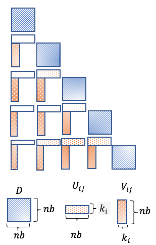
Figure 1: TLR representation of a covariance matrix ${\boldsymbol{\Sigma}}({\boldsymbol{\theta}})$ with fixed accuracy.

Figure 1 illustrates the TLR representation of a given covariance matrix ${\boldsymbol{\Sigma}}({\boldsymbol{\theta}})$. Following the same principle as dense tile algorithms [2], our covariance matrix ${\boldsymbol{\Sigma}}({\boldsymbol{\theta}})$ is divided into a set of square tiles. The Singular Value Decomposition (SVD), Randomized SVD (RSVD), or Adaptive Cross Approximation (ACA) may be used then to approximate each off-diagonal tile up to a user-defined accuracy threshold. This threshold is, in fact, application-dependent and enables to truncate and keep the most significant $k$ singular values and their associated left and right singular vectors, ${\boldsymbol{U}}$ and ${\boldsymbol{V}}$, respectively. The number $k$ is the actual rank and is determined on a tile basis, i.e., one should expect variable ranks across the matrix tiles. A low accuracy translates into small ranks (i.e., low memory footprint), and therefore, brings the arithmetic intensity of the overall algorithm close to the memory-bound regime. Conversely, a high accuracy generates large ranks (high memory-footprint), which increases the arithmetic intensity and makes the algorithm run in the compute-bound regime. Each tile $(i,j)$ can then be represented by the product of $U_{ij}$ and $V_{ij}$, with a size of $nb\times k$, where $nb$ represents the tile size. The tile size is a tunable parameter and has a direct impact on the overall performance, since it corresponds to the trade-off between arithmetic intensity and degree of parallelism.

The next section introduces the new extension of ExaGeoStat framework [2] toward TLR matrix approximations of the Matérn covariance functions and TLR matrix computations using the high performance HiCMA numerical library, in the context of MLE calculations.

VI ExaGeoStat Software Infrastructure

This work is an extension of our ExaGeoStat framework [2], a high performance framework for geospatial statistics in climate and environment modeling. In [2], we propose using full machine precision accuracy for maximum likelihood estimation. Besides demonstrating the hardware portability of the framework, one of the motivations was to provide a reference implementation for eventual performance and accuracy assessment against different approximation techniques. In this work, we extend the ExaGeoStat framework with a TLR approximation technique and assessing it with the full accuracy reference solution. ExaGeoStat sits on top of three main components: (1) the ExaGeoStat operational routines which generate synthetic datasets (if needed), solve the MLE problem, and predict missing values at non-sampled locations, (2) linear algebra libraries, i.e., HiCMA and Chameleon, which provide linear solvers support for the ExaGeoStat routines, and (3) a dynamic runtime system, i.e., StarPU [4], which orchestrates the adaptive execution of the main computational routines on various shared and distributed-memory systems.

Once the ExaGeoStat high-level tasks (i.e., matrix generation, log-determinant and solve operations) are defined with their respective data dependencies, StarPU can enroll the sequential code and may asynchronously schedule the various tasks on the underlying hardware resources. By abstracting the hardware complexity via the usage of StarPU, user-productivity may be enhanced since developers can focus on the numerical correctness of their sequential algorithms and leave the parallel execution to the runtime system. Thanks to an out-of-order execution, StarPU is also capable of reducing load imbalance, mitigating data movement overhead, and increasing occupancy on the hardware.

Last but not least, ExaGeoStat includes an optimization software layer (i.e., The NLopt library) to optimize the likelihood objective function.

VII Definitions of Synthetic and Real Datasets

In this study, we use both synthetic and real datasets to validate our proposed TLR ExaGeoStat on different hardware architectures.

Synthetic data are generated at irregular locations over a predefined region over a two-dimensional space  [16, 39]. The synthetic representation aims at generating spatial locations where no two locations are too close. The data locations are generated using $n^{1/2}(r-0.5+X_{rl},l-0.5+Y_{rl})$ for $r,l\in\{1,\dots,n^{1/2}\}$, where $n$ represents the number of locations, and $X_{rl}$ and $Y_{rl}$ are generated using a uniform distribution on ($-$0.4, 0.4).

A drawable example of 400 irregularly spaced grid locations in a square region is shown by Figure 2. We only use such a small example to highlight how we are generating spatial locations, however, this work uses synthetic datasets up to $10^{6}$ locations with a total covariance matrix size equals $10^{12}$ double precision elements – about $80$ TB of memory.

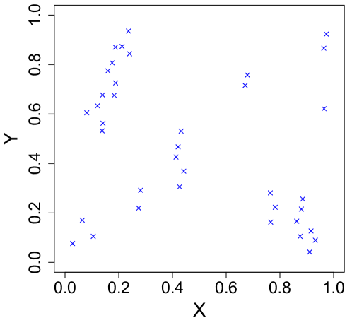
Figure 2: An example of $400$ points irregularly distributed in space, with 362 points ($\circ$) for maximum likelihood estimation and $38$ points ($\times$) for prediction validation.

Numerical models are essential tools to improve the understanding of the global climate system and the cause of different climate variations. Such numerical models are able to well describe the evolution of many variables related to the climate system, for instance, temperature, precipitation, humidity, soil moisture, wind speed and pressure, through solving a set of equations. The process involves physical parameterization, initial condition configuration, numerical integration, and data output. In this study, we use the proposed methodology to investigate the spatial variability of two different kinds of climate variables: soil moisture and wind speed.

Soil moisture is a key factor in evaluating the state of the hydrological process and has a wide range of applications in weather forecasting, crop yield prediction, and early warning of flood and drought. It has been shown that better characterization of soil moisture can significantly improve the weather forecasting. In particular, we consider high-resolution daily soil moisture data at the top layer of the Mississippi River Basin in the United States, on January 1st, 2004. The spatial resolution is of $0.0083$ degrees and the distance of one-degree difference in this region is approximately $87.5$ km. The grid consists of $1830\times 1329=2{,}432{,}070$ locations with 2,153,888 measurements and 278,182 missing values. We use the same model for the mean process as in Huang and Sun [16], and fit a zero-mean Gaussian process model with a Matérn covariance function to the residuals; see Huang and Sun [16] for more details on data description and exploratory data analysis.

Furthermore, we consider another example of climate and environmental data: wind speed. Wind speed is an important factor of the climate system’s atmospheric quantity. It is impacted by the changes in temperature, which lead to air moving from high-pressure to low pressure layers. Wind speed affects weather forecasting and different activities related to both air and maritime transportations. Moreover, constructions projects, ranging from airports, dams, subways and industrial complexes to small housing buildings are impacted by the wind speed and directions.

The advanced research core of WRF (WRF-ARW) is used in this study to generate a regional climate dataset over the Arabian Peninsula [40] in the Middle-East. The model is configured with a domain of a horizontal resolution of $5$ km with $51$ vertical layers while the model top is fixed at $10$ hPa. The domain covers the longitudes and latitudes of $20$°E - $83$°E and $5$°S - $36$°N, respectively. The data are available daily through $37$ years. Each data file represents $24$ hours measurements of wind speed recorded each hour on $17$ different layers. In our case, we have picked up one dataset on September 1st, 2017 at time 00:00 AM on a $10$-meter distance above ground (i.e., layer $0$). No special restriction is applied to the chosen data. We only choose an example to show the effectiveness of our proposed framework, but may easily consider extending the datasets.

Since ExaGeoStat can handle large covariance matrix computations, and the parallel implementation of the algorithm significantly reduces the computational time, we propose to use exact maximum likelihood inference for a set of selected regions in the domain of interest to characterize and compare the spatial variabilities of both the soil moisture and the wind speed data.

VIII Performance

This section evaluates the performance and the accuracy of the TLR ExaGeoStat framework for the MLE computations. It presents performance and accuracy assessments against the reference full accuracy implementation on shared and distributed-memory systems using synthetic and real datasets.

VIII-A Experimental Settings

We evaluate the performance of the TLR ExaGeoStat framework for the MLE computations on a wide range of Intel hardware systems’ generation to highlight our software portability: a dual-socket 28-core Intel Skylake Intel Xeon Platinum 8176 CPU running at 2.10 GHz, a dual-socket 14-core Intel Broadwell Intel Xeon E5-2680 V4 running at 2.4 GHz, a dual-socket 18-core Intel Haswell Intel Xeon CPU E5-2698 v3 running at 2.30 GHz, Intel manycore Knights Landing (KNL) 7210 chips with 64 cores, and a dual-socket 8-core Intel Sandy Bridge Intel Xeon CPU E5-2650 running at 2.00 GHz. For the distributed-memory experiments, we use Shaheen-2 from the KAUST Supercomputing Laboratory, a Cray XC40 system with 6,174 dual-socket compute nodes based on 16-core Intel Haswell processors running at 2.3 GHz. Each node has 128 GB of DDR4 memory. Shaheen-2 has a total of 197,568 processor cores and 790 TB of aggregate memory. In fact, our software portability is in fact guaranteed, as long as an optimized BLAS/LAPACK high performance library is available on the targeted system.

Our framework is compiled with gcc v5.5.0 and linked against latest Chameleon and HiCMA libraries with HWLOC v1.11.8, StarPU v1.2.1, Intel MKL v11.3.1, GSL v2.4, and NLopt v2.4.2 optimization libraries. All computations are carried out in double precision arithmetic and each run has been repeated three times. The accuracy and qualitative analyses are performed using synthetic and two examples of real datasets, i.e., the soil moisture dataset at Mississippi River Basin region and the wind speed dataset from the Middle-East region, as described in Section VII for more details.

VIII-B Performance on Shared-Memory Systems

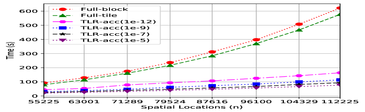
(a) A dual-socket $18$-core Intel Haswell.

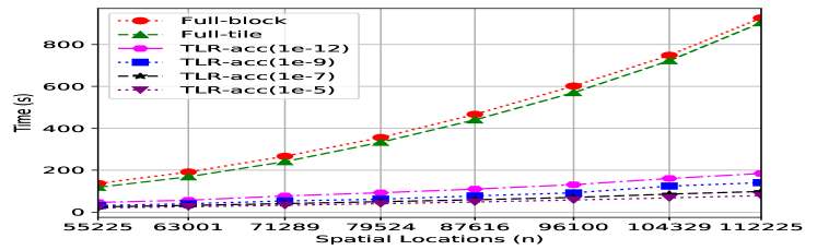
(b) A dual-socket $14$-core Intel Broadwell.

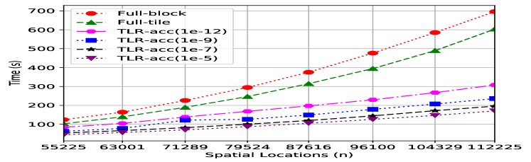
(c) $64$-core Intel Knights Landing (KNL).

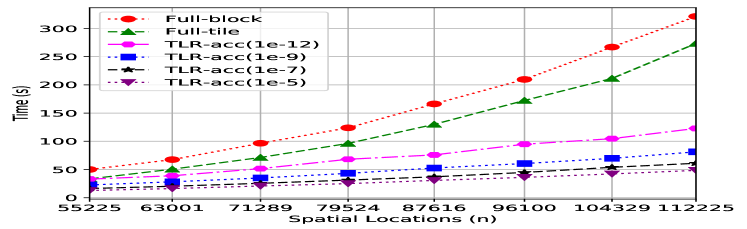
(d) A dual-socket $28$-core Intel Skylake.

Figure 3: Time of one iteration of the TLR MLE operation on different Intel architectures.

We present the performance analysis of TLR MLE computation on the four aforementioned Intel systems over various numbers of spatial locations. We compare against the full machine precision accuracy obtained from the block and tile MLE implementations, with the Intel MKL LAPACK and Chameleon libraries, respectively, as described in Section V. In the following figures, the x-axis represents the number of spatial locations, and the y-axis represents the total execution time in seconds. We use four different TLR accuracy thresholds, i.e., $10^{-5}$, $10^{-7}$, $10^{-9}$, and $10^{-12}$. Figure 3 shows the time to solution to perform the TLR MLE operation across generations of Intel systems. Since the internal optimization process is an iterative procedure, which usually takes a few tens of iterations, we only report the time for a single iteration as a proxy for the overall optimization procedure. The elapsed time for the full machine precision accuracy for the tile MLE outperforms the block implementations. This is expected and has already been highlighted in [2]. Regarding the TLR MLE implementations, the time to solution steadily diminishes as the requested accuracy decreases. This phenomenon is reproduced on all shared-memory platforms. The maximum speedup achieved by TLR MLE is significant for all studied accuracy thresholds. In particular, the maximum speedup obtained with $10^{-5}$ accuracy threshold is around $7$X, $10$X, $13$X and $5$X on the Intel Haswell, Broadwell, KNL and Skylake, respectively. The speedup numbers have to be cautiously assessed, since approximation obviously introduces numerical errors and may not be bearable by the geospatial statistics application beyond a certain threshold. So, the challenge is to maintain the model fidelity with high accuracy, just enough, to outperform the full machine precision accuracy MLE implementations by a non-negligible factor.

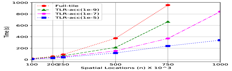
(a) $256$ nodes.

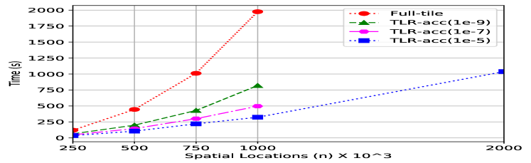
(b) $1024$ nodes.

Figure 4: Time of one iteration of the TLR MLE operation on Cray XC40 Shaheen-2 using different accuracy thresholds.

VIII-C Performance on Distributed-Memory Systems

We also test our TLR ExaGeoStat framework on the distributed-memory Shaheen-2 Cray XC40 system using $256$ ($\sim 8,200$ cores) and $1024$ nodes ($\sim 33,000$ cores), as highlighted in Figure 4. Similarly to the results on shared-memory systems, significant speedups (up to $5$X) are achieved when performing TLR ExaGeoStat approximations for the MLE computations using different numbers of spatial locations. There are some points missing in the graphs, which correspond to cases where the application runs out of memory. While this is the case when performing no TLR approximation, this may also occur with TLR approximation with high accuracy thresholds. Tuning the tile size $nb$ is of paramount importance to achieving high performance when running in approximation or full accuracy mode. For instance, for the full machine precision accuracy (i.e, full-tile) variant of the ExaGeoStat MLE calculations, we use a tile size of $560$, while a much higher tile size of $1900$ is required for the TLR variants to be competitive. This tile size discrepancy is due to the resulting arithmetic intensity of the main computational tasks for each variant. For the full-tile variant, since the main kernel is the dense matrix-matrix multiplication, $nb=560$ is large enough to keep single cores busy caching data located at the high level of the memory subsystem, and small enough to provide enough concurrency for the overall execution of the MLE application. For the TLR variants, large tile size is necessary, since the shape of the data structure depends on the actual rank obtained after compression. These ranks are usually much smaller than the tile size $nb$. Moreover, the main computational kernel for TLR MLE computations is the TLR matrix-matrix multiplication, which involves several successive linear algebra calls [5]. As a result, the resulting arithmetic intensity of that kernel is rather low, close to memory-bound regime. In distributed-memory systems, this mode translates into latency-bound since data motion happens between remote node memories. This engenders significant overheads, which can not be compensated since computation is very limited. We may therefore increase the tile size just enough to slightly shift the regime toward compute-bound, while preserving a high level of parallelism to maintain hardware occupancy. We tuned the tile size $nb$ on our target distributed-memory Shaheen-2 Cray XC40 system to gain the best performance of our MLE implementation.

Moreover, we investigate the performance of the prediction operation (i.e., $100$ unknown measurements), as introduced in equation (4). Figure 5 shows the execution time for the prediction on different synthetic datasets up to $1M\times 1M$ matrix size using $256$ nodes. The most time-consuming part of the prediction operation is the Cholesky factorization in this configuration, since the number of unknown measurements to calculate is rather small and triggers only a small number of triangular solves. Thus, the performance curves show a similar behavior as the MLE operation using the same number of nodes, as shown in Figure 4(a).

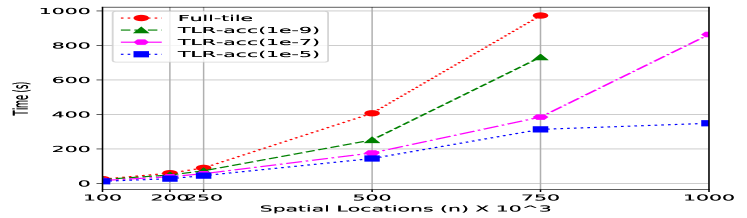
Figure 5: Time of TLR prediction operation on Cray XC40 Shaheen-2 with $256$ nodes.

VIII-D Accuracy Verification and Qualitative Analysis

We evaluate the accuracy of TLR approximation techniques for the MLE calculations with different accuracy thresholds and compare against its full machine precision accuracy variant. The accuracy can be verified at two different occasions: estimating the MLE parameter vector and predicting missing measurements at certain locations. Here, we use both synthetic and real datasets to perform this accuracy verification and analyze the effectiveness of the proposed approximation techniques.

VIII-D1 Synthetic Datasets (Monte Carlo Simulations)

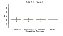
(a) Estimated variance parameter ($\theta_{1}$).

(b) Estimated spatial range parameter ($\theta_{2}$).

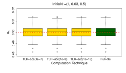
(c) Estimated smoothness parameter ($\theta_{3}$).

(d) Estimated variance parameter ($\theta_{1}$).

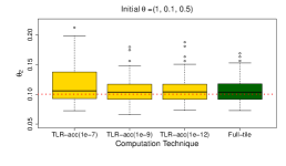
(e) Estimated spatial range parameter ($\theta_{2}$).

(f) Estimated smoothness parameter ($\theta_{3}$).

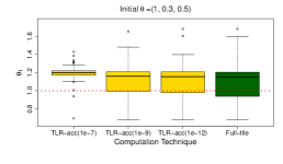
(g) Estimated variance parameter ($\theta_{1}$).

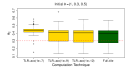
(h) Estimated spatial range parameter ($\theta_{2}$).

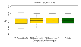
(i) Estimated smoothness parameter ($\theta_{3}$).

Figure 6: Boxplots of parameter estimation ($\theta_{1}$, $\theta_{2}$, and $\theta_{3}$).

The overall goal of the MLE model is to estimate the unknown parameters of the underlying statistical model $(\theta_{1},\theta_{2},\theta_{3})$ of the Matérn covariance function, then to use this model for future predictions. Monte Carlo simulation is a common way to estimate the accuracy of the MLE operation using synthetic datasets. ExaGeoStat data generator is used to generate synthetic datasets. The input of the data generator is an initial parameter vector to produce a set of locations and measurements. This initial parameter vector can be reproduced by the MLE operation using the generated spatial data. More details about the data generation process can be found in [2]. We generate a $40K$ synthetic data, one location matrix and 100 different measurement vectors, in exact computation. We rely on exact computation on this step to ensure that all techniques are using the same data for the MLE operation.

As described in Section IV, the Matérn covariance function depends on three parameters, variance $\theta_{1}$, range $\theta_{2}$, and smoothness $\theta_{3}$. The correlation strength can be determined using the range parameter $\theta_{2}$ (i.e., strong correlated data ($\theta_{2}=0.3$), medium correlated data ($\theta_{2}=0.1$), weak correlated data ($\theta_{2}=0.03$). These correlations values are restricted by the smoothness parameter ($\theta_{3}=0.5$). Thus, we select three combination of the three parameters, i.e., ($(1,0.3,0.5)$, $(1,0.1,0.5)$, and $(1,0.03,0.5)$). The correlation has obviously a direct impact on the compression rate, and therefore, the actual ranks of the TLR covariance matrix for the MLE computation.

Figure 6 shows three boxplots for each initial parameter vector representing the estimation accuracy using different computation techniques. The true value of each $\theta$ is denoted by a dotted red line. It is clearly seen from the figure that with weak correlation (i.e., $\theta_{2}=0.03$), TLR approximation is able to retrieve the initial parameter vector with the same accuracy as the exact computation.

The medium correlation (i.e., $\theta_{2}=0.1$) also shows better accuracy with TLR approximation up to accuracy $10^{-9}$. However, TLR with accuracy $10^{-7}$ is less compared to other accuracy levels. With stronger correlation (i.e., $\theta_{2}=0.3$), TLR with accuracy $10^{-7}$ and $10^{-9}$ are not able to retrieve the parameter vector efficiently. In this case, only TLR with accuracy $10^{-12}$ can be compared with the exact solution. In summary, TLR requires higher accuracy if the data is strongly correlated.

Prediction is key to checking the TLR approximation accuracy compared to the full-tile variant. Here, we conduct another experiment to predict $100$ missing values from synthetic datasets generated from our three parameter vectors (i.e., $(1,0.03,0.5)$, $(1,0.1,0.5)$, and $(1,0.3,0.5)$). The missing values are randomly picked from the generated data so that it can be used as a prediction accuracy reference. To assess the accuracy, we use the Mean Square Error (MSE) metric as follows:

$${\displaystyle\operatorname{MSE}={\frac{1}{100}}\sum_{i=1}^{100}(Y_{i}-{\hat{Y_{i}}})^{2}.}$$ (7)

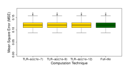
(a) Initial $\boldsymbol{\theta}$ vector $(1-0.03-0.5)$.

(b) Initial $\boldsymbol{\theta}$ vector $(1-0.1-0.5)$.

(c) Initial $\boldsymbol{\theta}$ vector $(1-0.3-0.5$).

Figure 7: Prediction mean square error (MSE) using synthetic datasets with three different parameter vector.

The three boxplots are shown in Figure 7. The TLR approximation variant perform well using the three accuracy thresholds (i.e., $10^{-7}$, $10^{-9}$, and $10^{-12}$) with different parameter vector. This demonstrates the effectiveness of TLR approximation with different data correlation degree in the prediction, even if the estimated parameter is not as accurate as the full-tile variant for some accuracy thresholds.

Another general observation for both TLR and full-tile variants, prediction MSE becomes lower in magnitude, if data is strongly correlated, as expected. For example, the average prediction MSE is $0.124$ in the case of weak correlated data (i.e., $(1,0.03,0.5)$ , $0.036$ in the case of medium correlated data (i.e., $(1,0.1,0.5)$), and $0.012$ in the case of strong correlated data (i.e., $(1,0.3,0.5)$).

VIII-D2 Real Datasets

Qualitative assessment using real datasets is critical to ultimately assess the effectiveness of TLR approximation for the MLE computations against the full-tile variant. Here, we use the two different datasets, introduced in Section VII.

Figure 8(a) shows the soil moisture dataset with $2$M locations. We divide the data map into eight regions, from R$0$ to R$7$ to reduce the execution time of estimating the MLE operation especially in the case of exact computation. Furthermore, Figure 8(b) shows the wind speed dataset with $1$M locations. As the soil moisture dataset, we chose to divide the wind speed map into four regions from R$0$ to R$3$. Generally, in both maps, each region contains about $250$K locations.

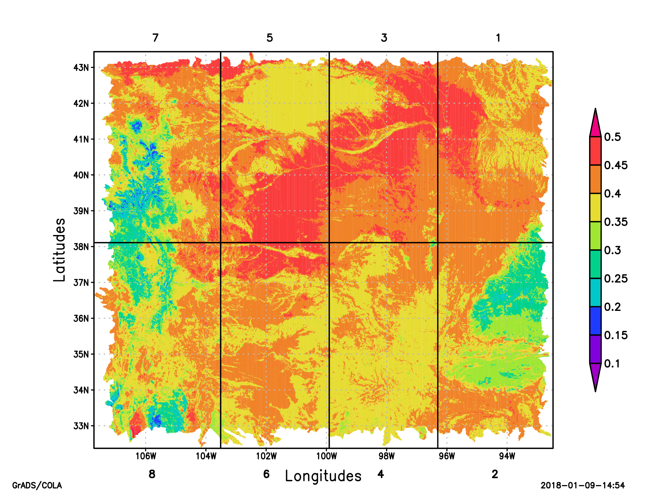
(a) Soil moisture data ($8$ geographical regions).

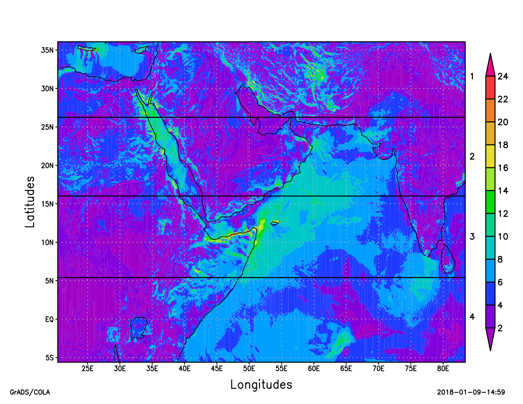
(b) Wind speed data ($4$ geographical regions).

Figure 8: Two examples of real geospatial datasets.

Tables I and II record the estimated parameters using TLR approximation techniques with different accuracy thresholds as well as the reference one obtained with full-tile variant. We report the estimated values to facilitate the reproducibility of this experiment. Using soil moisture datasets, we can use a TLR accuracy up to $10^{-12}$ which is still faster than full-tile technique while in wind speed dataset the highest accuracy used is $10^{-9}$ to maintain better performance compared to full-tile variant.

Both tables show that highly correlated regions require high TLR accuracy thresholds to reach the same parameter estimation quality as the full-tile variant, e.g., the soil moisture data, R$7$ and R$8$, and the wind dataset, R$1$, R$2$, and R$3$. Moreover, the results show that the smoothness parameter is the easiest parameter to be estimated with any TLR accuracy thresholds, even in presence of highly correlated data.

TABLE I: Estimation of the Matérn covariance parameters for $8$ geographical regions of the soil moisture dataset.

	Matérn Covariance
R	Variance ($\theta_{1}$)					Spatial Range ($\theta_{2}$)					Smoothness ($\theta_{3}$)
	TLR Accuracy					TLR Accuracy					TLR Accuracy
	$10^{-5}$	$10^{-7}$	$10^{-9}$	$10^{-12}$	Full-tile	$10^{-5}$	$10^{-7}$	$10^{-9}$	$10^{-12}$	Full-tile	$10^{-5}$	$10^{-7}$	$10^{-9}$	$10^{-12}$	Full-tile
R1	0.855	0.855	0.855	0.855	0.852	6.039	6.034	6.034	6.033	5.994	0.559	0.559	0.559	0.559	0.559
R2	0.383	0.378	0.378	0.378	0.380	10.457	10.307	10.307	10.307	10.434	0.491	0.491	0.491	0.491	0.490
R3	0.282	0.283	0.283	0.283	0.277	11.037	11.064	11.066	11.066	10.878	0.509	0.509	0.509	0.509	0.507
R4	0.382	0.38	0.38	0.38	0.41	7.105	7.042	7.042	7.042	7.77	0.532	0.533	0.533	0.533	0.527
R5	0.832	0.837	0.837	0.837	0.836	9.172	9.225	9.225	9.225	9.213	0.497	0.497	0.497	0.497	0.496
R6	0.646	0.615	0.621	0.621	0.619	10.886	10.21	10.317	10.317	10.323	0.521	0.524	0.524	0.524	0.523
R7	0.430	0.452	0.452	0.452	0.553	14.101	15.057	15.075	15.075	19.203	0.519	0.516	0.516	0.516	0.508
R8	0.661	1.194	0.769	0.769	0.906	18.603	37.315	22.168	22.168	27.861	0.469	0.462	0.467	0.467	0.461

TABLE II: Estimation of the Matérn covariance parameters for $4$ geographical regions of wind speed dataset.

	Matérn Covariance
R	Variance ($\theta_{1}$)				Spatial Range ($\theta_{2}$)				Smoothness ($\theta_{3}$)
	TLR Accuracy				TLR Accuracy				TLR Accuracy
	$10^{-5}$	$10^{-7}$	$10^{-9}$	Full-tile	$10^{-5}$	$10^{-7}$	$10^{-9}$	Full-tile	$10^{-5}$	$10^{-7}$	$10^{-9}$	Full-tile
R1	7.406	9.407	12.247	8.715	29.576	33.886	39.573	32.083	1.214	1.196	1.175	1.210
R2	11.920	13.159	13.550	12.517	26.011	28.083	28.707	27.237	1.290	1.267	1.260	1.274
R3	10.588	10.944	11.232	10.819	18.423	18.783	19.114	18.634	1.418	1.413	1.407	1.416
R4	12.408	17.112	12.388	12.270	17.264	17.112	17.247	17.112	1.168	1.170	1.168	1.170

Moreover, we estimate the prediction MSE of $100$ missing values, which are randomly chosen from the same region. We select two regions from each dataset, i.e., R$1$ and R$4$ from the soil moisture data, and R$1$ and R$3$ from the wind speed data. We conduct this experiment $100$ times and Figure 9 shows the four boxplots with different computation techniques. The figure shows that TLR approximation technique for MLE provides a prediction MSE close to the full-tile variant with different accuracy thresholds, even if the estimated parameters slightly differ, as shown in Tables I and  II.

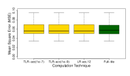
(a) Soil moisture data R1.

(b) Soil moisture data R3.

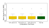
(c) Wind speed data R1.

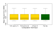
(d) Wind Speed data R4.

Figure 9: Prediction Mean Square Error (MSE) using Synthetic Datasets with three different parameter vector.

IX Conclusion

This paper introduces the Tile Low-Rank approximation into the open-source ExaGeoStat framework (TLR support to be released soon) for effectively computing the Maximum Likelihood Estimation (MLE) on various parallel shared and distributed-memory systems, in the context of climate and environmental applications. This permits to reduce the arithmetic complexity and memory footprint of MLE computations by exploiting the data sparsity structure of the Matérn covariance matrix of size up to $2$M. The resulting TLR approximation for the MLE computation outperforms its full machine precision accuracy counterpart up to $13$X and $5$X on synthetic and real datasets, respectively. A comprehensive qualitative assessment of the accuracy of the statistical parameter estimation as well as the prediction (i.e., supervised learning) demonstrates the limited compromise required to achieve high performance, while maintaining proper accuracy.

Acknowledgment. We would like to thank Intel for support in the form of an Intel Parallel Computing Center award and Cray for support provided during the Center of Excellence award to the Extreme Computing Research Center at KAUST. This research made use of the resources of the KAUST Supercomputing Laboratory.

References

- [1] M. L. Stein, “Interpolation of spatial data, some theory for kriging,” Springer Series in Statistics, 1999.
- [2] S. Abdulah, H. Ltaief, Y. Sun, M. G. Genton, and D. E. Keyes, “ExaGeoStat: A high performance unified framework for geostatistics on manycore systems,” arXiv preprint arXiv:1708.02835, 2017.
- [3] “The Chameleon project,” January 2017, available at https://project.inria.fr/chameleon/.
- [4] C. Augonnet, S. Thibault, R. Namyst, and P. Wacrenier, “StarPU: a unified platform for task scheduling on heterogeneous multicore architectures,” Concurrency and Computation: Practice and Experience, vol. 23, no. 2, pp. 187–198, 2011.
- [5] K. Akbudak, H. Ltaief, A. Mikhalev, and D. E. Keyes, “Tile Low Rank Cholesky Factorization for Climate/Weather Modeling Applications on Manycore Architectures,” in 32nd International Conference, ISC High Performance 2017, Frankfurt, Germany, June 18-22, 2017, Proceedings, ser. Lecture Notes in Computer Science, vol. 10266. Springer, 2017, pp. 22–40.
- [6] K. Akbudak, H. Ltaief, A. Mikhalev, A. Charara, and D. Keyes, “Exploiting data sparsity for large-scale matrix computations,” in Proceedings of the 24th International Conference on Euro-Par 2018: Parallel Processing. New York, NY, USA: Springer-Verlag New York, Inc., 2018.
- [7] Y. Sun, B. Li, and M. G. Genton, “Geostatistics for large datasets,” in Space-Time Processes and Challenges Related to Environmental Problems, M. Porcu, J. M. Montero, and M. Schlather, Eds. Springer, 2012, pp. 55–77.
- [8] C. K. Wikle and N. Cressie, “A dimension-reduced approach to space-time Kalman filtering,” Biometrika, vol. 86, no. 4, pp. 815–829, 1999.
- [9] J. M. Ver Hoef, N. Cressie, and R. P. Barry, “Flexible spatial models for kriging and cokriging using moving averages and the Fast Fourier Transform (FFT),” Journal of Computational and Graphical Statistics, vol. 13, no. 2, pp. 265–282, 2004.
- [10] S. Banerjee, A. E. Gelfand, A. O. Finley, and H. Sang, “Gaussian predictive process models for large spatial data sets,” Journal of the Royal Statistical Society: Series B (Statistical Methodology), vol. 70, pp. 825–848, 2008.
- [11] N. Cressie and G. Johannesson, “Fixed rank kriging for very large spatial data sets,” Journal of the Royal Statistical Society: Series B (Statistical Methodology), vol. 70, no. 1, pp. 209–226, 2008.
- [12] C. G. Kaufman, M. J. Schervish, and D. W. Nychka, “Covariance tapering for likelihood-based estimation in large spatial datasets,” Journal of the American Statistical Association, vol. 103, no. 484, pp. 1545–1555, 2008.
- [13] H. Sang and J. Z. Huang, “A full scale approximation of covariance functions for large spatial data sets,” Journal of the Royal Statistical Society: Series B (Statistical Methodology), vol. 74, no. 1, pp. 111–132, 2012.
- [14] C. Gu, Smoothing spline ANOVA models. Springer Science & Business Media, 2013, vol. 297.
- [15] M. L. Stein, J. Chen, and M. Anitescu, “Stochastic approximation of score functions for gaussian processes,” Annals of Applied Statistics, to appear, 2013.
- [16] H. Huang and Y. Sun, “Hierarchical low rank approximation of likelihoods for large spatial datasets,” Journal of Computational and Graphical Statistics, no. just-accepted, 2017.
- [17] W. Hackbusch, “A sparse matrix arithmetic based on-matrices. part i: Introduction to-matrices,” Computing, vol. 62, no. 2, pp. 89–108, 1999.
- [18] B. N. Khoromskij, A. Litvinenko, and H. G. Matthies, “Application of hierarchical matrices for computing the karhunen–loève expansion,” Computing, vol. 84, no. 1-2, pp. 49–67, 2009.
- [19] P. Ghysels, X. S. Li, F. Rouet, S. Williams, and A. Napov, “An efficient multicore implementation of a novel hss-structured multifrontal solver using randomized sampling,” SIAM Journal on Scientific Computing, vol. 38, no. 5, pp. S358–S384, 2016.
- [20] H. Pouransari, P. Coulier, and E. Darve, “Fast hierarchical solvers for sparse matrices using low-rank approximation,” arXiv preprint arXiv:1510.07363, 2015.
- [21] S. Börm and S. Christophersen, “Approximation of BEM matrices using GPGPUs,” arXiv preprint arXiv:1510.07244, 2015.
- [22] D. A. Sushnikova and I. V. Oseledets, “Compress and eliminate solver for symmetric positive definite sparse matrices,” arXiv preprint arXiv:1603.09133, 2016.
- [23] A. Aminfar and E. Darve, “A fast, memory efficient and robust sparse preconditioner based on a multifrontal approach with applications to finite-element matrices,” International Journal for Numerical Methods in Engineering, vol. 107, no. 6, pp. 520–540, 2016.
- [24] P. Amestoy, A. Buttari, J. L’Excellent, and T. Mary, “On the complexity of the block low-rank multifrontal factorization,” SIAM Journal on Scientific Computing, vol. 39, no. 4, pp. A1710–A1740, 2017.
- [25] G. Pichon, E. Darve, M. Faverge, P. Ramet, and J. Roman, “Sparse supernodal solver using block low-rank compression: design, performance and analysis,” Ph.D. dissertation, Inria Bordeaux Sud-Ouest, 2017.
- [26] P. Amestoy, A. Buttari, I. Duff, A. Guermouche, J. L’Excellent, and B. Uçar, MUMPS. Boston, MA: Springer US, 2011, pp. 1232–1238.
- [27] N. Cressie and C. K. Wikle, Statistics for spatio-temporal data. John Wiley & Sons, 2015.
- [28] M. G. Genton, “Separable approximations of space-time covariance matrices,” Environmetrics, vol. 18, no. 7, pp. 681–695, 2007.
- [29] B. Matérn, Spatial Variation, second edition ed., ser. Lecture Notes in Statistics. Berlin; New York: Springer-Verlag, 1986, vol. 36.
- [30] J. Chiles and P. Delfiner, Geostatistics: modeling spatial uncertainty. John Wiley & Sons, 2009, vol. 497.
- [31] S. Börm and J. Garcke, “Approximating Gaussian processes with -matrices,” in Proceedings of 18th European Conference on Machine Learning, Warsaw, Poland, September 17-21, 2007. ECML 2007, vol. 4701, 2007, pp. 42–53.
- [32] M. S. Handcock and M. L. Stein, “A Bayesian analysis of kriging,” Technometrics, vol. 35, pp. 403–410, 1993.
- [33] P. Guttorp and T. Gneiting, “Studies in the history of probability and statistics XLIX: On the Matérn correlation family,” Biometrika, vol. 93, pp. 989–995, 2006.
- [34] G. R. North, J. Wang, and M. G. Genton, “Correlation models for temperature fields,” Journal of Climate, vol. 24, pp. 5850–5862, 2011.
- [35] M. G. Genton, D. E. Keyes, and G. Turkiyyah, “Hierarchical decompositions for the computation of high-dimensional multivariate normal probabilities,” Journal of Computational and Graphical Statistics, no. https://doi.org/10.1080/10618600.2017.1375936, 2017.
- [36] D. Rick, “Deriving the haversine formula,” in The Math Forum, April, 1999.
- [37] E. Agullo, J. Demmel, J. Dongarra, B. Hadri, J. Kurzak, J. Langou, H. Ltaief, P. Luszczek, and s. Tomov, “Numerical Linear Algebra on Emerging Architectures: The PLASMA and MAGMA Projects,” Journal of Physics: Conference Series, vol. 180, no. 1, pp. 12–37, 2009. [Online]. Available: http://stacks.iop.org/1742-6596/180/i=1/a=012037
- [38] E. Anderson, Z. Bai, C. Bischof, L. S. Blackford, J. Demmel, J. Dongarra, J. Du Croz, A. Greenbaum, S. Hammarling, A. McKenney et al., LAPACK Users’ Guide. SIAM, 1999.
- [39] Y. Sun and M. L. Stein, “Statistically and computationally efficient estimating equations for large spatial datasets,” Journal of Computational and Graphical Statistics, vol. 25, no. 1, pp. 187–208, 2016.
- [40] W. C. Skamarock, J. B. Klemp, J. Dudhia, D. O. Gill, D. M. Barker, W. Wang, and J. G. Powers, “A description of the advanced research wrf version 2,” National Center For Atmospheric Research Boulder Co Mesoscale and Microscale Meteorology Div, Tech. Rep., 2005.