Small-angle X-ray scattering in amorphous silicon: A computational study

Abstract

We present a computational study of small-angle X-ray scattering (SAXS) in amorphous silicon (a-Si) with particular emphasis on the morphology and microstructure of voids. The relationship between the scattering intensity in SAXS and the three-dimensional structure of nanoscale inhomogeneities or voids is addressed by generating ultra-large high-quality a-Si networks with 0.1-0.3 % volume concentration of voids, as observed in experiments using SAXS and positron annihilation spectroscopy. A systematic study of the variation of the scattering intensity in the small-angle scattering region with the size, shape, number density, and the spatial distribution of the voids in the networks is presented. Our results suggest that the scattering intensity in the small-angle region is particularly sensitive to the size and the total volume-fraction of the voids, but the effect of the geometry or shape of the voids is less pronounced in the intensity profiles. A comparison of the average size of the voids obtained from the simulated values of the intensity, using the Guinier approximation and Kratky plots, with those from the spatial distribution of the atoms in the vicinity of void surfaces is presented.

I Introduction

Small-angle X-ray scattering (SAXS) is a powerful method for studying structural inhomogeneities on the extended length scale in solids and condensed-phase systems in solution. Guinier (1994); Feigin and Svergun (2013); Hura et al. (2009) While X-ray crystallography and nuclear magnetic resonance (NMR) spectroscopy can provide high-resolution structural information, small-angle scattering of X-rays and neutrons is particularly useful in probing low-resolution structural characteristics of partially-ordered and disordered objects on the nanometer length scale, which is often complemented with results from X-ray diffraction and NMR measurements. Mertens and Svergun (2010) Since its first inception by Guinier Guinier (1994) in the late 1930s, SAXS has been employed extensively in probing structural properties of a variety of crystalline and non-crystalline solids, including nanocomposites, alloys, glasses, ceramics, and polymers. Guinier (1994); Feigin and Svergun (2013); Glatter (1977) In recent years, the advancement of SAXS instrumentation and the availability of high-brilliance X-ray sources have led to the development and emergence of SAXS as a principal tool in structural biology Grant et al. (2011); Pérez and Nishino (2012) for studying an array of biological objects ranging from large macromolecules Putnam et al. (2007), biopolymers, Hyland et al. (2013) RNA folding, Pollack (2011); Doniach (2001) multi-domain proteins with flexible linkers, Bernado et al. (2007) and intrinsically disordered proteins. Bernado and Svergun (2012) In spite of the tremendous success and the widespread applications of SAXS in obtaining structural information on the size, shape, and compactness of the scattering objects (e.g., macromolecules in solution or voids in amorphous environments), a direct determination of the three-dimensional structure of the scatterers solely based on the information content of a given SAXS data set is impossible unless additional independent information is available to complement the SAXS data. Since the distribution of the scatterers produces a rotational averaging of the intensity in reciprocal space, the absence of directional (or phase) information between the scatterers makes it extremely difficult to unambiguously reconstruct the three-dimensional shape of a mono-disperse scattering object from one-dimensional intensity profiles. While the problem is more acute for poly-disperse objects in biomolecular systems, the analysis of SAXS data in structural biology is often accompanied by complementary structural information from high-resolution X-ray crystallography and NMR data, providing additional information on the structure of the constituents or sub-units of the scattering objects in order to develop a three-dimensional model. Zheng and Doniach (2002) Complications also arise in interpreting and translating experimental SAXS data from the reciprocal-space domain to the real-space domain owing to the finite size of the data set, sampled only at specific points in reciprocal space. In an authoritative treatment, Moore Moore (1980) has addressed this problem by developing a framework based on the sampling theorem of Shannon, Shannon and Weaver (1949) which provides an elegant ansatz to extract the full information content in a given data set and to estimate the errors associated with the parameters derived from the analysis.

Given the complexity involved in the analysis of experimental SAXS data and the subsequent determination of a three-dimensional model of the scattering objects, a natural approach to address the problem is to study the relationship between the SAXS intensity and the structure of scattering objects by directly simulating the scattering intensity from realistic model configurations, obtained from independent calculations. In this paper, we address the morphology of voids in a-Si with particular emphasis on the relationship between the (simulated) intensity from SAXS and the shape, size, density, and the spatial distribution of the voids in amorphous silicon. While the problem has been studied extensively using experimental SAXS data for a-Si and a-Si:H,Williamson et al. (1989); Mahan et al. (1991, 1989a); Acco et al. (1996) there exist only a few computational studies Biswas et al. (1989); Brahim and Chehaidar (2011) that have attempted to address the problem from an atomistic point of view using rather small models of a-Si, containing only 500 to 4000 atoms. Since the information that resides in the small-angle region of reciprocal space is connected to real space via the Fourier transformation, it is necessary to have a significantly large model to include any structural correlations that may originate from distant atoms in order to produce the correct long-wavelength behavior of the scattering intensity. Thus, accurate simulations of SAXS in non-crystalline solids were hampered in the past by the lack of appropriately large structural models of a-Si, with a linear size of several tens of angstroms, which are necessary for reliable computation of the scattering intensity in the small-angle region.

We should mention that an impressive number of computational and semi-analytical studies can be found in the literature from the past decades that address the relationship between the scattering intensity in SAXS and the morphological characteristics of inhomogeneities present in a sample, using the homogeneous-medium approximation. Guinier (1994); Letcher and Schmidt (1966); Moonen et al. (1989); Ilavsky and Jemian (2009) Such an approach, however, crucially relies on the assumption that the length scale ($l$) associated with the inhomogeneities is significantly larger than the atomic-scale structure ($R$) of the embedding medium (i.e., $l>>R$), so that any density fluctuations that may originate from the atomic-scale structure of the embedding matrix on the length scale of $R$ can be neglected for the computation of the intensity in the relevant small-angle region of interest. It thus readily follows that, given the length scale of the voids in a-Si ($l\approx$ 10–18 Å) and the atomic-scale structure of the amorphous-silicon matrix ($R\approx$ 10–15 Å), neither the homogeneous-medium approximation nor an approach based upon relatively small atomistic models of a-Si, consisting of 500–4000 Si atoms, is adequate for accurate simulations of SAXS intensity in the presence of nanometer-size inhomogeneities in amorphous silicon.

The importance of atomistic simulations becomes particularly apparent in determining the effect of surface relaxation on the shape of the inhomogeneities and its possible manifestation on SAXS intensities, which cannot be addressed realistically using the homogeneous-medium approximation. Furthermore, the behavior of the static structure factor in the small-angle limit is by itself an important topic for studying the long-wavelength density fluctuations in disordered systems. In an influential paper appearing in the Proceedings of the National Academy of Sciences, Xie et al. Xie et al. (2013) presented highly sensitive transmission X-ray scattering data of a-Si samples to examine the infinite-wavelength limit ($q\to 0$) of the structure factor $S(q)$ for determining the degree of hyperuniformity, and reported a value of $S(0)=0.0075\pm 0.0005$. Following these authors, $S(q\to 0)$ can be used as a figure-of-merit to study the quality of the amorphous-silicon network generated in our simulations. Here, we shall show that the value of $S(q\to 0)$ obtained from our simulations is closer to the experimental value than the computed value reported in the literature by de Graff and Thorpe. de Graff and Thorpe (2010) For a discussion on hyperuniformity and its applications to disordered systems, the readers may refer to the work by Torquato and co-workers. S. Torquato (2016); Kim and Torquato (2018)

The remainder of the paper is as follows. In Sec. II, we address the computational method associated with the production of ultra-large high-quality structural models of a-Si, which is followed by the calculation of the SAXS intensity and the construction of voids of different shapes, sizes, densities, and their spatial distributions in several model configurations of amorphous silicon. Section III discusses the results from our simulations where we address the characteristic structural properties of the models and compare the simulated structure factor with the high-resolution structure-factor data of a-Si from experiments. This is followed by a discussion on the restructuring of a void surface upon total-energy relaxation and the subsequent changes in the shape and topology of the surface atoms. Thereafter, we examine the relationship between the morphology of the voids and the scattering intensity in SAXS, by studying several models of a-Si with a varying size, shape, and concentration of the voids. A comparison of the size of the voids with the same obtained from the simulated intensity in the small-angle region is also presented from Guinier and Kratky plots. Section IV presents the conclusions of our work.

II Computational Methods

II.1 Large-scale modeling of a-Si for simulation of SAXS

Since the main purpose of the present work is to study the structure and statistical properties of extended-scale inhomogeneities on the nanometer length scale, we are interested in the scattering region associated with small wave vectors in the range of 0–1 Å^-1. For inhomogeneities, such as voids, with a typical size of $l\approx$ 10–20 Å, one needs to measure scattering intensities for the wave vectors in the vicinity of $k=2\pi/l\approx$ 0.3–0.6 Å^-1. This means that the appropriate structural models needed to be used in the simulation of small-angle X-ray scattering must have a linear dimension of several nanometers in order to compute statistically-reproducible physical quantities from the simulated SAXS data. To fulfill this requirement, we generated ultra-large atomistic configurations of a-Si using classical molecular-dynamics (MD) simulations, as described below.

Two independent initial configurations, each comprising $N=262,400$ Si atoms, were generated by randomly placing atoms in a cubic simulation box of length 176.12 Å, so that the minimum distance between any two Si atoms was 2.0 Å. This corresponds to a mass density of 2.24 g/cm³ for the models, which is identical to the experimental mass density of a-Si reported by Custer et al. Custer et al. (1994) Starting from these initial configurations, MD simulations were carried out in the canonical ensemble by describing the interatomic interaction between Si atoms using the modified Stillinger-Weber potential.Stillinger and Weber (1985); Vink et al. (2001) The equations of motion were integrated using the velocity-Verlet algorithm with a time step of $\Delta t=1$ fs and the Nosé-Hoover thermostatNosé (1984); Hoover (1985); Martyna et al. (1996) was employed to control the simulation temperature, with a thermostat period of $\tau=0.2$ ps. The initial temperature of each configuration was set to 1800 K and the configurations were equilibrated for 20 ps. After equilibration at 1800 K, each configuration was cooled to 300 K over a total time period of 300 ps with a cooling rate of 5 K/ps. Since atomistic models of amorphous silicon obtained from MD simulations, using a single heating-and-cooling cycle, cannot produce good structural properties owing to the large volume and dimensionality of the phase space in a limited simulation time, we repeated the heating-and-cooling cycles 30 times in order to sample the phase space extensively for producing high-quality atomistic configurations with excellent structural properties. For the present simulations, this translates into a total simulation time of 9 nanoseconds for each configuration. The final configurations were obtained by minimizing the total energy with respect to the atomic positions using the limited-memory BFGS algorithm.Nocedal (1980); Liu and Nocedal (1989) In the following, we refer to these final configurations as M-1 and M-2, and we have used them for further simulation and analyses of the scattering intensity in SAXS. The characteristic structural properties of these models are listed in Table 2.

II.2 Simulation of SAXS intensity for amorphous solids

For disordered and amorphous systems, the intensity of X-ray scattering is a function of the microscopic state of the system. The scattering intensity depends on the individual scattering units (e.g., atoms, molecules, cells) and the characteristic statistical distribution of the units in the system. The scattering intensity for a system consisting of $N$ atoms can be written as,

$$I({\mathbf{k}})=\sum_{i}^{N}\sum_{j}^{N}f_{i}({\mathbf{k}})f_{j}({\mathbf{k}})\exp[\imath{\mathbf{k}}\cdot(\mathbf{r}_{i}-\mathbf{r}_{j})],$$ (1)

where the contribution from an individual atom enters through the atomic form-factor $f_{i}({\mathbf{k}})$ and the structural information follows from the (positional) distribution of the constitutent atoms in the system. Here, the wave-vector transfer, ${\mathbf{k}}$, is the difference between the scattered ($\mathbf{k}_{f}$) and incident ($\mathbf{k}_{i}$) wave vectors, and its magnitude is given by $k=|\mathbf{k}_{f}-\mathbf{k}_{i}|=4\pi\sin\theta/\lambda$, where $2\theta$ and $\lambda$ are the scattering angle and the wavelength of the incident X-ray radiation (e.g., 1.54 Å for the Cu K_α line), respectively. While Eq. (1) can be evaluated directly for small systems, it is computationally very demanding and infeasible to compute the intensity for large models with hundreds of thousands of atoms. Since it is necessary to minimize surface effects by imposing the periodic boundary conditions, one needs to evaluate the double sum in Eq. (1) in order to compute the intensity values. Further, the computation of the configurational-averaged values of the scattering intensity, for a given $k$, requires angular averaging over all possible directions of ${\mathbf{k}}$ over a solid angle of $4\pi$. Finally, using the well-known sampling theorem of Shannon, Shannon and Weaver (1949) it can be shown that, in order to extract the full information content of SAXS data, one must sample the scattering intensity at equally-spaced points, $k_{i}$, with spacing $\Delta k$ – also known as Shannon channels – such that $\Delta k\leq\pi/l$, where $l$ is the maximum linear size of the inhomogeneities dispersed in the system. Moore (1980); Damaschun et al. (1968) These considerations lead to the conclusion that, for a system with $10^{5}$ atoms, one requires to compute approximately 10¹⁵ or more operations in order to obtain the intensity plot from Eq. (1). The conventional approach is to carry out the averaging procedure analytically by introducing a pair-correlation function $g(r)$, which is associated with the probability of finding an atom at a distance $r$, given that there is an atom at $r=0$. By invoking the assumptions that the system is homogeneous and isotropic and that the strong peak near $k$=0, originating from a constant density term, does not provide any structural information and thus can be removed from consideration, one arrives at the following expression for the scattering intensity for a monatomic system,

$$I_{N}(k)=Nf^{2}(k)\,S(k),$$ (2)

where

$$S(k) = 1+\frac{4\pi\rho}{k}\int_{0}^{\infty}r(g(r)-1)\,\sin{kr}\,dr$$ (3)

$$\approx 1+\int_{0}^{R}r\,G(r)\,\frac{\sin{kr}}{kr}\,dr.$$

In Eq. (3), we have introduced the reduced distribution function, $G(r)=4\pi\rho\,r(g(r)-1)$. For computational purposes, it is also necessary to replace the upper limit of the integral by a large but finite cutoff distance, $R$, beyond which $(g(r)-1)$ tends to vanish. For finite-size models, the cutoff distance, $R$, is generally, but not necessarily, chosen to be the half of the box length for a cubic model of linear size $L$. Equation (3) can be readily employed to compute the structure factor reliably in the wide-angle limit but the difficulty remains for very small values of $k$. It has been shown by Levashov et al.Levashov et al. (2005) that $g(r)$ converges to unity very slowly, and at finite temperature there exist small but intrinsic fluctuations, even for a very large value of $R$. In the small-angle limit, the term $\sin(kr)/kr$ in Eq. (3) changes very slowly but the fluctuations in $r\,G(r)$ grow considerably beyond a certain radial distance $R_{c}$ due to the presence of the $r^{2}$ term. Thus, $R_{c}$ must be as large as possible to extract structural information for small $k$ values. It is often convenient to write Eq. (3) in two parts by introducing a damping factor $\gamma(r)$ in the region $r\geq R_{c}$. The resulting equation now reads,

$$S(k)\approx 1+\int_{0}^{R_{c}}rG(r)\frac{\sin{kr}}{kr}dr+\int_{R_{c}}^{R}\gamma(r)rG(r)\frac{\sin{kr}}{kr}dr.$$ (4)

Computational studies on $G(r)$ in a-Si, using large simulated models, indicate that the optimum value of $R_{c}$ is of the order of 30–40 Å. Beyond this distance, it is difficult to distinguish $G(r)$ from numerical noise and the accuracy of the integral in Eq. (3) is found to be affected by the presence of growing oscillations in $rG(r)$. To mitigate the effect of the truncation of the upper limit of the integral at small $k$ values, we have used an exponential damping factor, $\gamma(r)=\exp[-(r-R_{c})/\sigma]$, in the region $r\geq R_{c}$. Numerical experiments indicate that a choice of $R_{c}$ = 35–40 Å and $\sigma$ = 1 Å is appropriate for our models. Since structural information on extended-scale inhomogeneities generally resides beyond the first few neighboring shells, this observation implies that, even with very large models, one must be careful to interpret the simulated values of the scattering intensity below $k=2\pi/R_{c}\approx 0.1$ Å^-1 due to a low signal-to-noise ratio in $rG(r)$, as shown in Fig. 1. Once the structure factor is available, the reduced scattering intensity, $I(k)$, can be obtained from the expression,

$$I(k)=\frac{I_{N}(k)}{N}=f^{2}(k)S(k),$$ (5)

where $N$ is the number of atoms in the model. The atomic form-factor can be obtained from the International Tables for CrystallographyWilson (1993) or from a suitable approximated form of $f(k)$.Doyle and Turner (1968); Smith and Burge (1962) At a finite temperature $T$, the expression for the reduced intensity in Eq. (5) is multiplied by the Debye-Waller (DW) factor, Debye (1913); Waller (1923) $\exp(-2M)$, where $M=(8\pi^{2}\sin^{2}{\theta}/\lambda^{2})(u^{2}/3)$ and $u^{2}(T)$ is the mean-square displacement of Si atoms in the amorphous state at temperature $T$. The Debye-Waller-corrected reduced intensity can be written as,

$$I_{DW}(k,T)=\exp(-2M)\,I(k).$$ (6)

The calculation of the Debye-Waller factor for the amorphous state is, by itself, an interesting problem and it is related to the vibrational dynamics of the atoms at a given temperature. The factor plays an important role in extracting structural information from X-ray scattering data by reducing and redistributing the scattering intensity at high temperature. At room temperature, the DW factor affects the intensity values only marginally for small values of $k$ and it can be replaced by unity for the computation of scattering intensity in the region $k<$ 1.0 Å^-1.

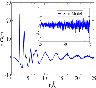
Figure 1: The variation of $r\,G(r)$ with $r$ for the M1 model of a-Si containing 262,400 atoms. The inset shows the growing fluctuations in $r\,G(r)$ beyond 40 Å, which affect the evaluation of the integral in Eq. 3. See Sec. IIB for a discussion.

II.3 Geometry of voids in a-Si for SAXS simulation

In order to examine the relationship between the morphology of voids and the intensity of the small-angle X-ray scattering in a-Si, it is necessary to construct a variety of void distributions in a-Si networks, which are characterized by different shapes, sizes, and number densities of voids. Since experimental data from IR, NMR, SAXS, Williamson (1995); Mahan et al. (1989a); Chabal and Patel (1987); Williamson et al. (1989); Mahan et al. (1989b) positron annihilation spectroscopy (PAS), Muramatsu et al. (1994); Wang et al. (2016); Melskens et al. (2017) and implanted helium-effusion measurements Beyer (2004); Beyer et al. (2011) suggest that the percentage of void-volume fraction ($f_{v}$) in a-Si and a-Si:H varies from 0.1% to 0.3% of the total volume of the samples, and the typical size or radius of the voids ranges from 5 Å to 10 Å, we have restricted ourselves to generating structural models of a-Si with voids that simultaneously satisfy both the requirement of void-volume fraction and the size of the voids. Toward that end, we have created several void distributions, which are characterized by spherical, ellipsoidal, and cylindrical voids, by randomly generating void centers within two model networks, M-1 and M-2, consisting of 262,400 Si atoms in a cubic simulation cell of length 176.12 Å. To ensure that the randomly-generated void distributions in the networks are as realistic as one observes in experiments, we introduced three characteristic lengths, $R_{v}$, $d$, and $D$, as illustrated in Fig. 2. The radius of a spherical void is given by $R_{v}$, whereas $d$ indicates the width of the spherical concentric region between radii $R_{v}$ and $R_{v}+d$, which determines the interface region of the (spherical) void and the bulk network. Silicon atoms in this region will be referred to as interface atoms, and we shall see later that these atoms play an important role in the relaxation of void surfaces. The atoms within a void region are removed from the system in order to produce an empty cavity or a void. $D$ indicates the minimum interface-to-interface distance between two neighboring voids, as shown in Fig. 2. This implies that the center-to-center distance, $r_{ij}$, between two spherical voids at sites $i$ and $j$ satisfies the constraint $r_{ij}\geq 2(R_{v}+d)+D$. By choosing appropriate values of $f_{v}$, $R_{v}$, and $D$, one can produce a variety of void distributions, which are consistent with experimental results as far as the void-volume fraction and the size of the voids are concerned.

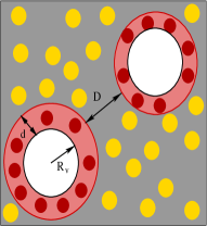
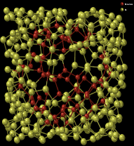
Figure 2: A schematic representation of voids in two dimensions (left) showing the characteristic lengths associated with void size ($R_{v}$), interface width ($d$), and the surface-to-surface distance ($D$) between two voids. The figure on the right-hand side shows a spherical void of radius 6 Å in a network of size 10 Å. For visual clarity, the silicon atoms on the void surface, having an interface width of $d$ = 2.8 Å, and the bulk region are shown in red and yellow colors, respectively.

For example, by choosing a large (or small) value of $D$, one can construct a sparse (or clustered) distribution of voids. Throughout the study, we have used $d$ = 2.8 Å that corresponds to the maximum nearest-neighbor distance between two silicon atoms in a-Si. For a given set of $f_{v}$, $R_{v}$, $D$, and the shape of the voids, one can compute the number of voids $n_{v}=f_{v}V/\nu$, where $\nu$ and $V$ are the volumes associated with an individual void and the simulation cell, respectively. For non-spherical voids, such as ellipsoidal and cylindrical voids, we replace $R_{v}$ by appropriate lengths $R_{v}^{e}$ and $R_{v}^{cy}$, which indicate the geometric mean radius of an ellipsoidal void and the cross-sectional radius of a cylindrical void, respectively. Ellipsoidal voids were generated by constructing triaxial ellipsoids with the axes ratios $a:b:c$ = $\frac{R_{v}}{2}:R_{v}:2R_{v}$, so that the geometric mean radius $R_{v}^{e}$ (=$\sqrt[3]{abc}$) is equal to the radius $R_{v}$ of a spherical void for a given $f_{v}$. For cylindrical voids, the height of a cylinder was taken to be three times its cross-sectional radius, $R_{cy}$, and the latter was chosen so that the volume of the cylinder was identical to that of a sphere or an ellipsoid (see Ref. Kra, ). The orientations of the ellipsoidal and cylindrical voids were randomly generated by constructing a three-dimensional unit random vector from the center of each void and aligning the major axis of an ellipsoid or a cylinder along that direction. An example of a spherical void of radius $R_{v}$ = 6 Å and interface width of $d$ = 2.8 Å is shown in Fig. 2, which is embedded in a region of the a-Si network of linear dimension 10 Å. The silicon atoms in the bulk and interface regions of the void are shown in yellow and red colors, respectively.

Table 1: Characteristic properties of a-Si models with void distributions used in this work. $R$, $N_{b}$, $N_{s}$, and $N_{v}$ indicate the actual radius, and the total number of bulk, surface, and void atoms, respectively. The percentage void-volume fraction ($f_{v}$), number density per cm³ ($n_{\rho}$), and the average radius of gyration ($R_{g}$) of the voids are listed. See text for the nomenclature of the models listed below.

Model	$R$ (Å)	$N_{b}$	$N_{v}$	$N_{s}$	$f_{v}$	$n_{\rho}\times 10^{19}$	$R_{g}$ (Å)
SP6-R6	6.0	261584	259	557	0.1	0.11	6.13
SP3-R8	8.0	261634	306	460	0.1	0.05	8.09
SP12-R6	6.0	260761	533	1106	0.2	0.22	6.13
SP5-R8	8.0	261126	508	766	0.2	0.09	8.09
SP18-R6	6.0	259936	801	1663	0.3	0.33	6.13
SP8-R8	8.0	260371	819	1210	0.3	0.15	8.09
EL6-R6	6.0	261491	260	649	0.1	0.11	7.3
EL3-R8	8.0	261563	302	535	0.1	0.05	9.66
EL12-R6	6.0	260578	502	1320	0.2	0.22	7.31
EL5-R8	8.0	261005	513	882	0.2	0.09	9.66
EL18-R6	6.0	259666	763	1971	0.3	0.33	6.15
EL8-R8	8.0	260173	825	1402	0.3	0.15	9.66
CY6-R5	4.58	261731	260	409	0.1	0.11	5.83
CY3-R6	6.10	261752	298	350	0.1	0.05	7.73
CY12-R5	4.58	261065	511	824	0.2	0.22	5.78
CY5-R6	6.10	261327	494	579	0.2	0.09	7.74
CY18-R5	4.58	260389	774	1237	0.3	0.33	5.8
CY8-R6	6.10	260696	792	912	0.3	0.15	7.75
SP18-D1-R6	6.0	259935	789	1676	0.3	0.33	6.13
SP18-D8-R6	6.0	259948	785	1667	0.3	0.33	6.13
SP18-D14-R6	6.0	259949	795	1656	0.3	0.33	6.09

Table 1 lists some characteristic features of voids and the resulting models obtained by incorporating voids of different shapes, sizes, numbers, and void-volume fractions. In order to produce a statistically-significant number of voids for a given volume fraction of voids, the radii of the voids were restricted to 5–8 Å. For $f_{v}$ = 0.1%, 0.2%, and 0.3%, spherical, ellipsoidal and cylindrical voids of different sizes were generated randomly within the networks in such a way that none of the voids was too close to the boundary of the networks. In this work, we have studied a total of 21 models that are listed in column 1 of Table 1. Each of the models is indicated by its shape, the number of voids present in the model, and the approximate linear size of the voids. For example, EL6-R6 indicates a model with 6 ellipsoidal voids of radius 6 Å. Similarly, SP18-D8-R6 implies a model with 18 spherical voids of radius 6 Å, which are separated by the surface-to-surface distance ($D$) of at least 8 Å. For cylindrical voids, the exact value of the cross-sectional radius of a void is given in column 1 of Table 1. The total number of bulk ($N_{b}$), surface ($N_{s}$), and void voi ($N_{v}$) atoms, along with the corresponding void-volume fraction ($f_{v}$), number density of voids per cm³ ($n_{\rho}$), and the average radius of gyration ($R_{g}$) of the voids for each model after total-energy relaxation are also listed in Table 1. The average radius of gyration, $R_{g}$, of voids in a model configuration can be obtained from the atomic coordinates of all the interface atoms in a model.

III Results and Discussion

In the preceding sections, we have seen that the structural information from extended length scales chiefly resides in the small-angle scattering region of wave vectors, $k\leq$ 1.0 Å^-1. In view of our earlier observation that the computed values of the structure factor could be affected by finite-size effects, owing to the growing oscillations in $rG(r)$ at large $r$, it is necessary to examine the accuracy of the simulated values of the scattering intensity before addressing the relationship between the scattering intensity and the inhomogeneities or voids from SAXS measurements.

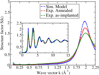
Figure 3: The structure factors of a-Si obtained from experiments and the present simulations. High-resolution experimental data at small $k$ for as-implanted and annealed samples of a-Si, from Ref. Xie et al., 2013, are indicated in green and red colors, respectively, while the simulated data, averaged over M-1 and M-2 configurations, are shown in blue. The full structure factors are presented in the inset, with the corresponding experimental data (using the same color coding) from Ref. Laaziri et al., 1999.

To this end, we shall compute the structure factor from model a-Si networks and compare the same with high-resolution experimental structure-factor data of a-Si reported recently in the literature.Xie et al. (2013); Laaziri et al. (1999)

III.1 Structure factor of a-Si in the small-angle scattering region

In Table 2, we have listed the characteristic structural properties of two models of a-Si, M-1 and M-2, as mentioned earlier in section IIA. Each of the models consists of 262,400 atoms in a cubic simulation cell of length 176.12 Å, which translates into an average mass density of 2.24 g/cm³. The average bond angle of 109.23^∘ between the nearest-neighbor atoms is found to be very close to the ideal tetrahedral value of 109.47^∘, with a root-mean-square deviation of $\sim$9.2^∘. The average Si-Si bond distance is observed to be about 2.39 Å, which is slightly higher than the experimental value Filipponi et al. (1989) of 2.36 Å and the theoretical value of 2.38 Å reported from ab initio calculations. Štich et al. (1991) The number of coordination defects is found to be somewhat higher (2.6%) than the values observed in high-quality WWW Wooten et al. (1985) or ART Barkema and Mousseau (1996) models obtained from event-based simulations but significantly lower than the structural models of a-Si obtained from earlier ab initio and classical molecular-dynamics simulations.Štich et al. (1991); md_ We shall see later in this section that the presence of a small percentage of coordination defects, which are sparsely distributed in the models on the atomistic length scale of 2–3 Å, do not affect the scattering intensity in the long-wavelength limit.

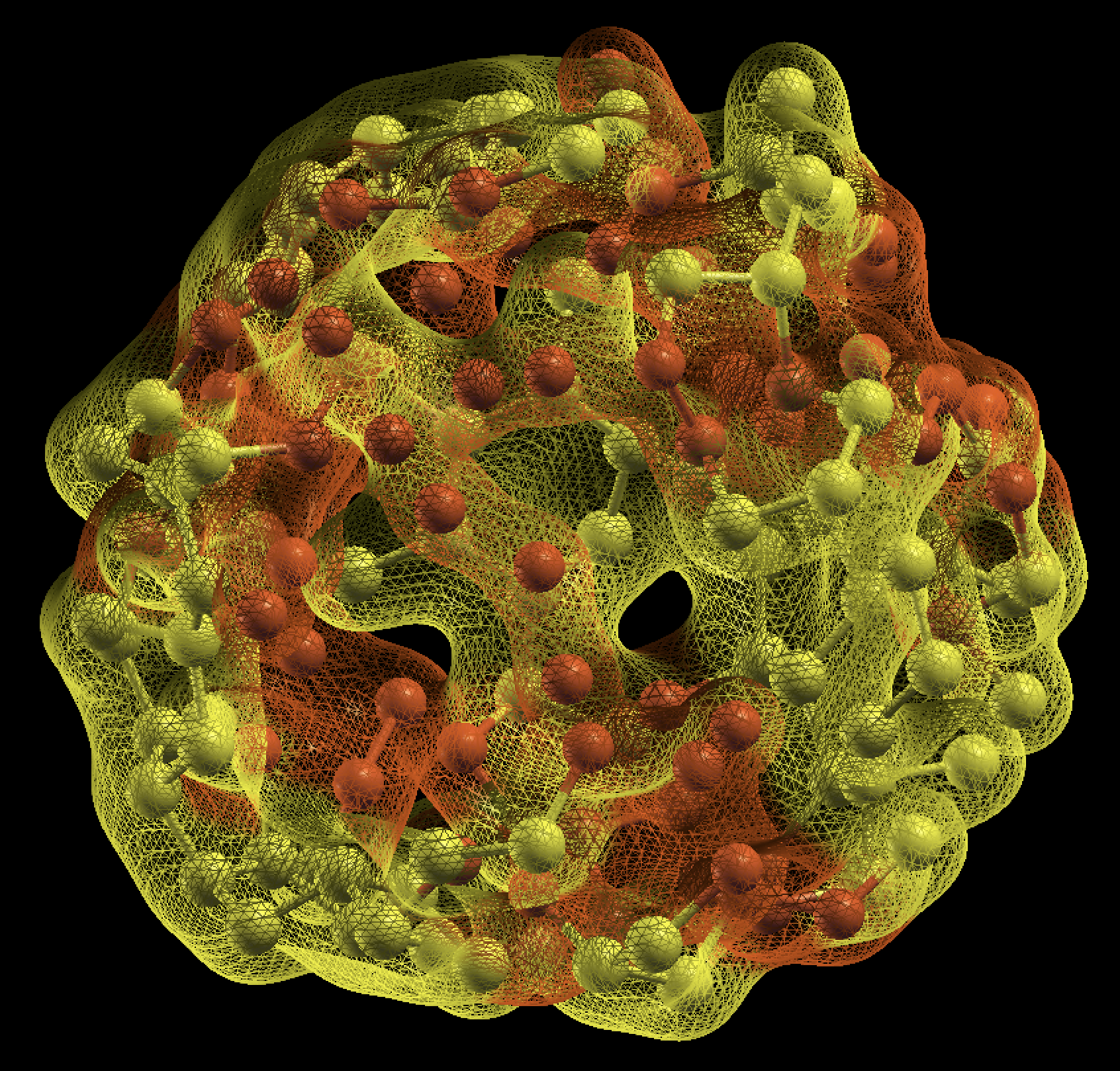
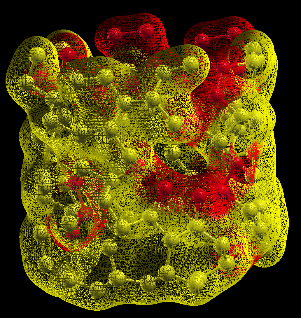
Figure 4: Reconstruction of a spherical void surface (in the SP18-R6 model) and a cylindrical void surface (in the model CY8-R6 model) during total-energy relaxation. For visual clarity, the interface atoms within a thin shell of width 2.8 Å and the associated reconstructed surfaces are shown in the plot. The red patches on the surfaces indicate the regions which are significantly reconstructed via the displacement of Si atoms (red) by more than 15% of the average Si-Si bond length.

Table 2: Structural properties of a-Si models used in the present study. $L$ = Simulation box length (Å), $\rho$ = mass density (g/cm³), $C_{4}$ = number of four-fold coordinated atoms (%), $d_{\text{Si}}$ = Average Si-Si bond length (Å), $\theta_{\text{avg}}$ = Average bond angle (degree), and $\Delta\theta_{\text{RMS}}$ = Root-mean-square deviation (degree).

Model	$N$	$L$	$\rho$	$C_{4}$	$d_{\text{Si}}$	$\theta_{avg}$	$\Delta\theta_{\text{rms}}$
M-1	262400	176.12	2.24	97.4	2.39	109.23∘	9.26∘
M-2	262400	176.12	2.24	97.4	2.39	109.23∘	9.20∘

Having addressed the structural properties of the models, we now examine the structure factor, $S(k)$, of a-Si in the small-angle region. Figure 3 presents $S(k)$ obtained by averaging the results from the model networks M-1 and M-2. The corresponding experimental data for as-implanted and annealed samples of a-Si, from Ref. Xie et al., 2013, are also plotted for comparison. Several observations are now in order. First, the simulated structure factor agrees well with the experimental data obtained from the annealed and as-implanted samples for $k$ values up to 15 Å^-1, as shown in the inset of Fig. 3. Second, an inspection of the simulated and experimental data in the vicinity of 1–2 Å^-1 reveals that the former is closer to the annealed data than to the as-implanted data. This observation is consistent with the expectation that a-Si models from MD simulations should be structurally and energetically closer to annealed samples than to as-implanted samples. Annealing of as-implanted samples at low to moderate temperature (400–500 K) reduces the network imperfection locally and thereby enhances the local ordering, which reflects in the first peak of $S(k)$. Third, it is notable that the models have reproduced the structure factor in the small-$k$ region, 0.15 $\leq$ $k\leq$ 1 Å,^-1 quite accurately, despite the presence of an artificial damping term in Eq. (4) that imposes an effective cutoff length of $R_{c}+5\,\sigma$ ($\approx$ 35–40 Å) on the radial correlation function and the presence of a small number of coordination defects.

While a direct comparison of the simulated structure factor (of a-Si) with its experimental counterpart establishes the efficacy of the numerical approach and the reliability of the models used in our study, a more stringent test to determine the accuracy of structure-factor data in the small-$k$ region follows from the behavior of $S(k)$ in the long-wavelength limit. de Graff and Thorpe de Graff and Thorpe (2010) addressed the problem computationally by analyzing $S(k)$ as $k\to$ 0, and concluded that $S(0)$ was of the order of 0.035 $\pm$ 0.001 by studying large a-Si models containing 10⁵ atoms. Likewise, an analysis of the high-resolution experimental structure-factor data of a-Si in the small-angle limit, presented in Fig. 3, by Xie et al. Xie et al. (2013) indicated a value of $S(0)\approx$ 0.0075 $\pm$ 0.0005 from experiments. Although a full analysis of the behavior of $S(k)$ near $k$ = 0 is outside the scope of the present work and will be addressed elsewhere, an extrapolation of $S(k)$ at $k$ = 0, by employing a second-degree polynomial fit in $k$ in the region 0.15–1.0 Å^-1, yields a value of 0.0154 $\pm$ 0.0017 in the present study. This value is comparable to the computed/experimental values mentioned earlier and is a reflection of the fact that our models produce accurate structure-factor data in the small-angle scattering region. The degree of hyperuniformity of a continuous-random-network model is often indicated by the value of $S(k)$ at $k$ = 0; a low value of $S(0)$ reflects a high degree of hyperuniformity. Xie et al. (2013); Hejna et al. (2013); S. Torquato (2016); de Graff and Thorpe (2010)

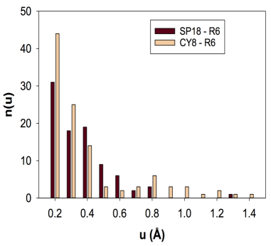
Figure 5: The distribution of atomic displacements ($u$) of the interface atoms on a void surface in the models SP18-R6 and CY8-R6 after total-energy relaxation. For clarity and comparison, only those values of the displacement with $u>$ 0.1 Å are shown above.

III.2 Reconstruction of void surfaces

Recent studies on hydrogenated a-Si, using ab initio density-functional simulations Biswas et al. (2017, 2014); Biswas and Elliott (2015) and experimental data from SAXS, Williamson et al. (1989) IR, Chabal and Patel (1987); Mahan et al. (1989a) and implanted helium-effusion measurements, Beyer (2004); Beyer et al. (2011) indicate that the shape of the voids in a-Si:H can be rather complex and that it depends on a number of factors, such as the size, number density, spatial distribution and the volume fraction of voids, and the method of preparation and conditions of the samples/models. While the experimental probes can provide considerable structural information on voids, it is difficult to infer the three-dimensional structure of voids from scattering measurements only. More importantly, experimental data from small-angle X-ray and neutron scattering measurements include, in general, contributions from an array of inhomogeneities with varying shapes and sizes, so it is difficult to ascertain the individual role of various factors in determining the shape of the measured intensity curve in small-angle scattering. In contrast, simulation studies are free from such constraints and capable of addressing systematically the effect of different shapes, sizes, number densities and the nature of distributions (e.g., isolated vs. interconnected) of voids/extended-scale inhomogeneities on scattering intensities. Before addressing these important issues, we shall first examine the restructuring of a spherical and a cylindrical void surface and the resulting changes of its shape due to atomic rearrangements on the surface or interface region of the voids.

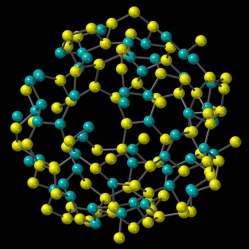
Figure 6: Local topological restructuring of a void surface (in the SP18-R6 model) via a change of atomic-coordination numbers. The silicon atoms, whose coordination number has increased [from (2,3) to (3,4)] during the restructuring process are indicated in light blue color.

Figure 4 shows the reconstructed void surfaces of a spherical void of radius 6 Å in the model SP18-R6 and a cylindrical void of cross-sectional radius 6.1 Å and height 18.3 Å in the model CY8-R6. As stated in section IIC, a spherical void is defined as an empty cavity of radius $r$ (6 Å for SP18-R6) with an interface width $d$ (2.8 Å). Atoms within the region between radii $r$ and $r+d$ are defined as the surface or interface atoms. A cylindrical cavity or void can be defined in a similar way. The radius of gyration of an assembly of surface atoms can be readily obtained from the atomic positions before and after total-energy relaxation to determine the degree of reconstruction and the shape of the void. For SP18-R6 and CY8-R6, it has been observed that approximately 50% and 30% of the total surface atoms moved from their original position by more than 0.36 Å or 15% of the average Si-Si bond length, respectively, indicating significant rearrangements of the surface atoms on the voids. A similar observation applies to the rest of the void models, where approximately (20–50)% of the interface atoms have been observed to participate in surface reconstruction. The interface atoms on a void surface in the models SP18-R6 and CY8-R6 are shown in Fig. 4 in red colors, along with the heavily reconstructed regions of the surface as red patches. The displacement of the interface atoms from their original position are presented in Fig. 5 by showing the distribution of the atomic-displacement values. Such a reconstruction of a void surface reduces the strain in the local network and increases the local atomic coordination via topological rearrangements. Figure 6 shows several atoms (in light blue color) on the surface of a void in model SP18-R6, whose coordination number has been found to increase from 2–3 to 3–4 upon total-energy relaxation. The effect of void-surface relaxations on the scattering intensity can be readily observed by computing the intensity before and after the relaxation. The results for the model SP18-R6 are shown in Fig. 7. It is apparent that the scattering intensity changes considerably upon total-energy relaxation despite the fact that the one-dimensional scattering intensity can carry only limited information associated with three-dimensional structural relaxation of voids.

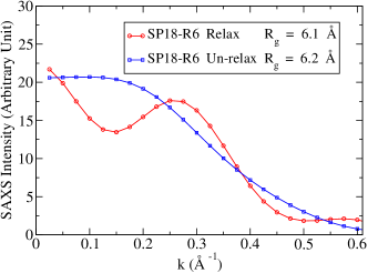
Figure 7: The effect of relaxation on the shape of the scattering curve for the model SP18-R6. The variation of the scattering intensity results from the three-dimensional restructuring of spherical void surfaces, as shown in Fig. 4(left).

III.3 Dependence of SAXS intensity on the size and volume fraction of voids

Experimental SAXS data on pure and hydrogenated a-Si suggest that the scattering intensity in the small-angle region is sensitive to the size and the total volume fraction of voids present in the samples. Williamson et al. (1995); Mahan et al. (1989a); Williamson et al. (1989); Acco et al. (1996) Here, we have studied the variation of the scattering intensity for different void volume fractions by introducing nanometer-size voids of spherical, ellipsoidal, and cylindrical shapes in model a-Si networks. Since the scattering intensity from an individual void is proportional to the volume of the void, it is necessary to choose spherical/ellipsoidal/cylindrical voids of an identical volume to ensure that any variation of the intensity can be solely attributed to the total volume fraction of the voids.

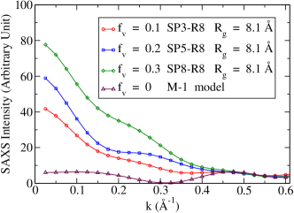
Figure 8: The variation of the scattering intensity (from Eq. 5) for four different void-volume fractions. For comparison, voids of an identical shape (i.e., spherical) and size but of different numbers were employed in the simulations. The average radii of gyration of the voids are indicated.

Following experimental observations,Williamson et al. (1995); Williamson (1995) we chose void-volume fractions in the range 0.1–0.3% by generating different number of voids of identical volumes and shapes. Figure 8 shows the intensity variation for four different values of the void-volume fraction with an identical individual volume of spherical voids. For small values of $k$, the scattering intensity strongly depends on the volume fraction of the voids and it increases steadily with increasing values of the void-volume fraction from 0.1% to 0.3%. Similar observations have been noted for ellipsoidal and cylindrical voids but are not shown here. Likewise, the effect of void sizes on the shape of the intensity curve in a-Si can be addressed in an analogous manner by introducing voids of different sizes at a given volume fraction of voids. The results for spherical and cylindrical voids for $f_{v}$ = 0.3% are presented in Fig. 9. An examination of the simulated data presented in Figs. 9(a) and 9(b) show that there is a noticeable variation in the scattering intensity in the small-$k$ region below 0.4 Å^-1 for both spherical and cylindrical voids.

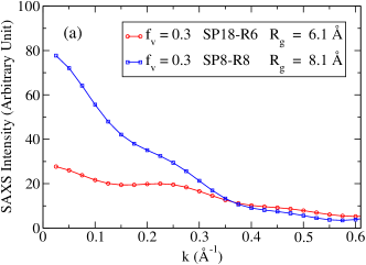
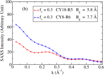
Figure 9: The simulated values of the scattering intensity for two different void sizes with 0.3% volume fraction of the voids. The results for spherical and cylindrical voids are shown in (a) and (b), respectively. The average radii of gyration ($R_{g}$) and the total volume fraction of the voids ($f_{v}$) are indicated in the plots.

III.4 Effect of void shapes on SAXS: Kratky plots for a-Si

In this section, we have studied the intensity plots for a-Si with spherical, ellipsoidal, and cylindrical voids for an identical total volume fraction of the voids to examine the effect of the shape and the spatial distribution of the voids on the scattering intensity in the small-angle region. Since the volume of an individual void can affect the scattering intensity considerably, we chose the size of the voids in such a way that the individual volumes of the voids were identical as far as the total number of missing atoms (in a void) is concerned. Figure 10 shows the variation of the scattering intensities with the wave vector for three models with different void shapes, averaged over two independent configurations for each model. Specifically, we have employed the models SP8-R8, EL8-R8, and CY8-R6. Each of the models contains 8 voids and has a total volume fraction of voids of 0.3%. Although the average radii of gyration of the voids are somewhat different in these models, the individual volume of the voids is kept constant to ensure that they contribute equally to the total scattering intensity. It is evident from Fig. 10 that the scattering intensity is not particularly sensitive to the shape of the void as long as the total volume fraction, individual void volume, and the number of voids are identical. This observation is consistent with the earlier experimental studies on a-Si:H by Mahan et al., Mahan et al. (1989a, b) Leadbetter et al., Leadbetter et al. (1981) and the study by Young et al., Young et al. (2007) where a weak dependence of the nature of the scattering curve on the shape of the voids or inhomogeneities was reported by tilting the incident beam with respect to the samples. In the next paragraph, we will see that a more effective approach to determine the effect of void shapes on the scattering intensity follows from studying Kratky plots, obtained from voids of different shapes.

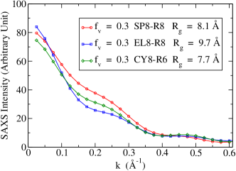
Figure 10: The dependence of the scattering intensity on the shape of the voids for a given total volume-fraction of voids in a-Si. The simulated values of the intensity for spherical (SP), ellipsoidal (EL), and cylindrical (CY) voids, having an identical value of the individual void-volume, are shown.

To examine the relationship between the shape of voids and the scattering intensity more closely, we have studied the variation of $k^{2}\,I_{c}(k)$ with $k$, which is often referred to as a Kratky plot in the literature. Glatter and Kratky (1982) Here, following the standard convention in the literature, $I_{c}(k)$ is the background-corrected intensity, which is obtained by subtracting the scattering contribution from the amorphous-silicon matrix with no voids. The quantity $k^{2}I_{c}(k)$ can be viewed as a $k$-space analog of $rG(r)$, which is more sensitive to the intensity variation than the conventional intensity $I(k)$, in the same manner as $rG(r)$ is more sensitive to structural ordering then the radial pair-correlation function $g(r)$. In recent years, Kratky plots have been used extensively in studying the structure of biological macromolecules in solution. It has been observed that, for compact and globular (i.e., spherical) proteins, the variation of $k^{2}I_{c}(k)$ with $k$ is distinctly different and stronger than for ones in the partially disordered and/or unfolded states. Kikhney and Svergun (2015); Burger et al. (2016) Specifically, a globular protein in the folded state exhibits an approximate semi-circular variation of $k^{2}I_{c}(k)$ with $k$, which gradually dissipates or flattens out as the degree of structural disorder increases and the protein becomes partially disordered by unfolding itself. Following this observation, one may expect that the shape-dependence of the scattering intensity on a Kratky plot would be more pronounced for spherical voids than that for long cylindrical or highly elongated ellipsoidal voids (see Refs. Mertens and Svergun, 2010 and not, ).

Figure 11 shows the variation of $k^{2}\,I_{c}(k)$ for spherical (SP), ellipsoidal (EL), and cylindrical (CY) voids. The results can be understood qualitatively as follows. Since the largest dimension (length) associated with the spherical, ellipsoidal, and cylindrical voids are given by $2R$, $4R$, and $2.3R$ (see Ref. Kra, ), respectively, where $R$ is the radius of a spherical void, it is not unexpected that the intensity variation is most pronounced for the spherical voids and vice versa for the (elongated) ellipsoidal voids. Deschamps and De Geuser Deschamps and De Geuser (2011) have shown that the peak position(s) ($k_{max}$) in a Kratky plot is (are) related to the pseudo-Guinier radius, $R_{pg}=\sqrt{3}/k_{max}$, in metallic systems, where the particle-size dispersion is usually large. The approach has been recently adopted by Claudio et al. Claudio et al. (2014) to estimate the size of silicon nanocrystals in bulk nanocrystalline (nc)-doped silicon from small-angle neutron-scattering data in order to study the effect of nanostructuring on the lattice dynamics of nc-doped silicon. Likewise, Diaz et al. Diaz et al. (2008) employed in situ SAXS for the detection of globular Si nanoclusters of size 20-30 Å during silicon film deposition by mesoplasma chemical vapor deposition. The SAXS intensity profiles obtained by these authors are more or less similar to the one obtained by us for the spherical voids. The pseudo-Guinier radii obtained from the peak positions in the scattering intensity for the spherical, ellipsoidal, and cylindrical voids are indicated in Fig. 11. The pseudo-Guinier radius of 6.7 Å, obtained from the Kratky plot in Fig. 11, for the spherical voids, matches closely with the initial radius of 8 Å before relaxation. For ellipsoidal and cylindrical voids, the presence of two peaks is clearly visible in the respective Kratky plots, which correspond to linear sizes of (3.8,7.7)Å and (4.3,6.9)Å, respectively. The presence of multiple peaks in a Kratky plot is indicative of a non-spherical shape of scattering objects. The lengths associated with these peaks are comparable to the ideal values of (4, 8)Å (minor and major axes) for ellipsoidal voids and (6, 9)Å (cross-sectional radius and height) for cylindrical voids before relaxation. We shall see in section 3F that the values of the pseudo-Guinier radii are also quite close to the values obtained from a conventional Guinier approximation and the average radii of gyration computed from the spatial distribution of the interface atoms in the vicinity of voids in a model.

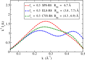
Figure 11: Kratky plots showing the variation of the background-correct $k^{2}I_{c}(k)$ with $k$ for spherical (SP), ellipsoidal (EL), and cylindrical (CY) voids of identical volumes and a total void-volume fraction. The pseudo-Guinier radii ($R_{pg}$) correspond to the $k$ values obtained from the peak position(s) of the intensities for different void shapes.

III.5 Effect of spatial distributions of voids on SAXS

In this section, we address the effect of spatial distributions of voids on the shape of the intensity curve in SAXS. Before discussing our results, we make the following observation. The application of the homogeneous-medium approximation in the dilute concentration limit of the inhomogeneities or particles, such that the particles are spatially well-separated, with a maximum linear size of $l$, suggests that the scattering intensity for monodisperse particles solely depends upon the volume ($V(l)$), number density ($N(l)$) and the shape of the particle for a given density difference ($\Delta\rho$) between the particles and the average density of the medium. Following Guinier Guinier (1994) and others, Letcher and Schmidt (1966); Moonen et al. (1989); Elliott (1990) the scattering intensity in this approximation can be expressed as,

$$I(k)=(\Delta\rho)^{2}\,V(l)\,N(l)\int_{0}^{l}4\pi r^{2}\gamma_{o}(r)\,\frac{\sin(kr)}{kr}\,dr,$$ (7)

where $\gamma_{o}(r)$ is a characteristic shape function of the particle whose value lies between 0 and 1. The expression in Eq. (7) suggests that the scattering intensity is independent of the atomic-scale structure of the embedding medium, provided that the maximum linear size of the particles ($l$) is significantly larger than the length scale ($R$) associated with the atomistic structure of the medium, i.e., $l>>R$. Given that $l\approx R\approx$ 10-18 Å in the present study, it thus follows that the criterion for the homogeneous-medium approximation is not satisfied adequately and that a dependence of the scattering intensity on the spatial distribution of voids may be expected.

The effect of the spatial distribution of the voids on the scattering intensity can be studied conveniently by generating a number of suitable isolated and clustered distributions of voids in real space. Since the microstructure of thin-film amorphous silicon is characterized by the presence of voids, which cause local fluctuations in the (mass) density, it is important to examine to what extent a sparse or interconnected distribution of voids can affect the scattering intensity in pure and hydrogenated amorphous silicon. Using implanted helium-effusion measurements, Beyer et al. Beyer (2004); Beyer et al. (2011) have shown that the presence of He-effusion peaks at low and high temperatures are associated with the diffusion of He atoms through an interconnected void region and the trapping of He atoms in a network of isolated voids, respectively. These authors have further noted that unhydrogenated samples of a-Si, prepared by vacuum evaporation, can have a high concentration of isolated voids. To examine this, we have studied a number of models with different spatial distributions of voids. By using three different surface-to-surface distances ($D$ = 1, 8, 14 Å), we have produced three void distributions consisting of 18 voids and of radius 6 Å. Each distribution corresponds to a volume-fraction density of 0.3% of voids and is reflective of a sparse distribution of voids, as one observes in hot-wire or plasma-deposited films of a-Si:H at low concentrations of hydrogen. Figure 12 shows the scattering intensity as a function of the wave vector obtained for these void distributions. While it is apparent that the intensity is not strongly sensitive to the void distribution, it is quite pronounced in the region of $k$ below 0.1 Å^-1 and in the vicinity of 0.26 Å^-1 for smaller values of $D$. A similar observation has been noted for the model CY18-R6 but the results are not shown here. This dependence can be attributed to the local density fluctutaions and the interaction between neighboring voids, which can originate from a clustered or interconnected distribution of voids produced by a small value of $D$. This is particularly likely in a-Si:H at high concentrations of hydrogen, where the void distribution has been observed to be highly interconnected both from experiments Beyer (2004); Beyer et al. (2011) and ab initio simulations. Biswas et al. (2017); Biswas and Elliott (2015) However, since the values of the intensity for $k<$ 0.1 Å^-1 is sensitive to the numerical noise in $G(r)$ and the real-space cutoff $R_{c}$, it is difficult to determine the behavior of the scattering intensity for wave vectors below 0.1 Å^-1. Thus, it would not be inappropriate to conclude that the scattering intensity is noticeably affected by the spatial distribution of voids, especially for a sparse distribution, for a given void-volume fraction in the small-angle region of $k\geq$ 0.1 Å^-1.

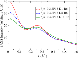
Figure 12: The dependence of the scattering intensity on the spatial distribution of the voids in a-Si for a given volume fraction and size of the voids. The surface-to-surface distance ($D$) between the voids is indicative of the degree of sparseness of the void distribution. Higher values of $D$ correspond to a more scattered or sparse distribution of voids.

III.6 Guinier approximation and the size of the inhomogeneities from SAXS

In writing Eq. (2) from (1) in section IIB, we have noted that a peak in $S(k)$, represented by a delta function,del at $k=0$ was excluded explicitly to arrive at the expression for the static structure factor. The exclusion of the central peak can be readily justified in experiments by recognizing that the (central) peak, being dependent on the external shape of the sample, is extremely narrow and thus it practically coincides with the incident beam. Analogously, one may invoke a similar assumption in the computer simulation of SAXS by employing a large but finite-size model of amorphous solids so that the computed values of the intensity at small $k$ are minimally affected. Guinier Guinier (1994) has shown that, for a homogeneous distribution of particles (e.g., voids) in the dilute limit, the scattering intensity for small values of $k$ can be approximated as, Guinier (1994)

$$I(k)=I(0)\exp\left(-\frac{k^{2}r_{g}^{2}}{3}\right),$$ (8)

provided that the particles are distributed randomly with all possible orientations and $kr_{g}<1$. In Eq. (8), $r_{g}$ is the radius of gyration of the particles and the inter-particle interaction is neglected owing to the dilute nature of their distribution. This relationship between the intensity and the wave vector in the small-angle limit is widely known as the Guinier approximation and it is frequently used in the experimental determination of the size of scattering objects on the nanometer length scale. The approximation suggests that, as long as the voids are distributed randomly (within a large model) in a dilute environment, one should be able to estimate the size of the voids from the shape of the intensity curve for small values of $k$. In practice, the calculation of the scattering intensity from Eq. (8) is constrained by the effective cutoff distance ($R_{c}$) of the reduced pair-correlation function and the size ($l$) of the inhomogeneities, which determine the lower and upper limits of $k$ in the Guinier approximation, respectively. For the present simulations, these values translate to an approximate $k$-range from 0.1 Å^-1 to 0.5 Å^-1.

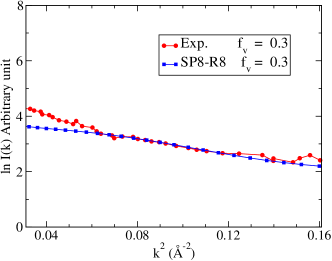
Figure 13: Guinier plots showing a comparison of the experimental SAXS data on a-Si, from Ref. Williamson, 1995, with the simulated values for a void-volume fraction of 0.3%.

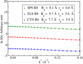
Figure 14: Guinier plots for the simulated values of the intensity for spherical (SP), ellipsoidal (EL), and cylindrical (CY) voids for a volume fraction of 0.3%. $R_{g}$ and $r_{g}$ refer to the radius of gyration obtained from the distribution of the interface atoms and the best-fit Guinier plots, respectively. For visual clarity, the results for the ellipsoidal (blue) and cylindrical (green) voids were given a vertical offset of -5 and 5 units, respectively.

Figure 13 shows a comparison of the experimental data from Ref. Williamson, 1995 with the results obtained from our simulations for a void-volume fraction of 0.3% on a Guinier plot, where, following Eq. (8), the scattering intensity is plotted on a natural log scale as a function of $k^{2}$. The simulated values of the intensity match closely with the experimental data, except for very small values of $k^{2}$ below 0.05 Å^-2. The deviation for small values of $k$ is not unexpected; it can be attributed partly to the difficulty in extracting information beyond $R_{c}$ from the reduced pair-correlation function and in part to the intrinsic differences between the simulated models and experimental samples. Since the latter generally include, depending upon the method of preparation and experimental conditions, voids of sizes from 5 Å to 15 Å, it is difficult to compare simulated data with experimental results at a quantitative level for very small values of $k$. The Guinier approximation in Eq. (8) suggests that the approximate size of the voids/inhomogeneities can be obtained from the slope of a $\ln I(k)$ vs. $k^{2}$ plot. To this end, we have plotted $\ln I(k)$ as a function of $k^{2}$ in Fig. 14 for spherical, ellipsoidal, and cylindrical voids. Since the values of the intensity are close to each other for different shapes, the results for the ellipsoidal and cylindrical voids are offset by +5 and -5 units, respectively, for the clarity of presentation. The radii of gyration obtained from the slopes of the fitted plots are indicated as $r_{g}$, whereas $R_{g}$ reflects the average value of the gyrational radius computed from the real-space distribution of the interface atoms of a void. Evidently, the latter is larger than the actual size of the void. For the purpose of comparison, we have subtracted 1.4 Å – a length equal to the half of the interface width $d$ – from the value obtained from the Guinier plot and have listed the corresponding corrected values for each model in the plots and in Table 1. It may be noted that $R_{g}$ values provide an upper bound of the average radius of gyration of the voids, whereas $r_{g}$ values of the same obtained from the Guinier plots might have been underestimated in our work owing to a possible deviation from the Guinier approximation in the scattering region of 0.1 to 0.6 Å^-1.

IV conclusions

Small-angle X-ray scattering is a powerful and versatile technique for the low-resolution structural characterization of inhomogeneities over a length scale of a few nanometers for a variety of ordered and disordered materials. In this work, we have presented a computational study of small-angle X-ray scattering in amorphous silicon, with particular emphasis on the shape, size, number density, total volume fraction, and the spatial distribution of voids in amorphous silicon. Since it is difficult to control these factors during experimental sample preparation and hence the analysis of the effect of these factors on experimental SAXS data, a direct simulation of the scattering intensity is particularly useful in studying the variation of the simulated SAXS intensity with respect to these factors using atomistic models of amorphous silicon. For the accurate simulation of the scattering intensity in the small-angle region down to 0.1 Å^-1, we have produced high-quality molecular-dynamical (MD) models containing 262,400 atoms that correspond to the experimental mass density of 2.24 g/cm³ for amorphous silicon. The MD models exhibited a narrow bond-angle distribution with an average bond angle of 109.23^∘$\pm$9.2^∘ and 97.4% four-fold coordinated atoms. The static structure factors obtained from these models agreed quite accurately with high-resolution experimental structure-factor data, obtained from transmission X-ray scattering measurements. The models exhibited a high-degree of hyperuniformity, characterized by the value of $S(k\to 0)\approx 0.0154\pm 0.0017$, which compares well with the value of 0.0075 extracted from the experimental structure-factor data.

An extensive analysis of the simulated SAXS data, obtained by varying the size, shape, and the volume fraction of voids introduced in the a-Si models, suggests that the scattering intensity is particularly sensitive to the size and the total volume fraction of the voids present in the models. The scattering intensity increases steadily with an increase of the size of the voids, irrespective of the shape and total volume fraction of the voids. While the shape dependence is less pronounced in the $I(k)$ vs. $k$ plots and is consistent with experimental SAXS data, an analysis of background-corrected $k^{2}I_{c}(k)$ vs. $k$ (Kratky) plots for spherical, ellipsoidal, and cylindrical voids reveals a clearer picture of the overall shape of the voids than the conventional intensity versus wave vector plots. The size of the voids obtained from the Guinier approximation and the Kratky plots are more or less consistent with each other and comparable with the values computed from the real-space distribution of the interface atoms, provided that the skin depth of the void-surfaces is taken into account.

V acknowledgments

This work was partially supported by the U.S. National Science Foundation under Grants No. DMR 1507166, No. DMR 1507118, and No. DMR 1506836. We acknowledge the Texas Advanced Computing Center at the University of Texas at Austin for providing HPC resources that have contributed to the results reported in this work.

References

References

- Guinier (1994) A. Guinier, X-Ray Diffraction In Crystals, Imperfect Crystals, and Amorphous Bodies (Dover Publications, Inc., New York, 1994).
- Feigin and Svergun (2013) L. Feigin and D. Svergun, Structure Analysis by Small-Angle X-Ray and Neutron Scattering (Springer US, 2013).
- Hura et al. (2009) G. L. Hura, A. L. Menon, M. Hammel, R. P. Rambo, F. L. Poole II, S. E. Tsutakawa, F. E. Jenney Jr, S. Classen, K. A. Frankel, R. C. Hopkins, S.-j. Yang, J. W. Scott, B. D. Dillard, M. W. W. Adams, and J. A. Tainer, Nature Methods 6, 606 EP (2009).
- Mertens and Svergun (2010) H. D. Mertens and D. I. Svergun, Journal of Structural Biology 172, 128 (2010).
- Glatter (1977) O. Glatter, Journal of Applied Crystallography 10, 415 (1977).
- Grant et al. (2011) T. D. Grant, J. R. Luft, J. R. Wolfley, H. Tsuruta, A. Martel, G. T. Montelione, and E. H. Snell, Biopolymers 95, 517 (2011).
- Pérez and Nishino (2012) J. Pérez and Y. Nishino, Current Opinion in Structural Biology 22, 670 (2012).
- Putnam et al. (2007) C. D. Putnam, M. Hammel, G. L. Hura, and J. A. Tainer, Quarterly Reviews of Biophysics 40, 191 285 (2007).
- Hyland et al. (2013) L. L. Hyland, M. B. Taraban, and Y. B. Yu, Soft Matter 9, 10218 (2013).
- Pollack (2011) L. Pollack, Biopolymers 95, 543 (2011).
- Doniach (2001) S. Doniach, Chemical Reviews 101, 1763 (2001).
- Bernado et al. (2007) P. Bernado, E. Mylonas, M. V. Petoukhov, M. Blackledge, and D. I. Svergun, Journal of the American Chemical Society 129, 5656 (2007).
- Bernado and Svergun (2012) P. Bernado and D. I. Svergun, Mol. BioSyst. 8, 151 (2012).
- Zheng and Doniach (2002) W. Zheng and S. Doniach, Journal of Molecular Biology 316, 173 (2002).
- Moore (1980) P. B. Moore, Journal of Applied Crystallography 13, 168 (1980).
- Shannon and Weaver (1949) C. E. Shannon and E. Weaver, The Mathematical Theory of Communication (University of Illinois Press, 1949).
- Williamson et al. (1989) D. L. Williamson, A. H. Mahan, B. P. Nelson, and R. S. Crandall, Journal of Non-Crystalline Solids 114, 226 (1989).
- Mahan et al. (1991) A. H. Mahan, Y. Chen, D. L. Williamson, and G. D. Mooney, Journal of Non-Crystalline Solids 137, 65 (1991).
- Mahan et al. (1989a) A. H. Mahan, D. L. Williamson, B. P. Nelson, and R. S. Crandall, Phys. Rev. B 40, 12024 (1989a).
- Acco et al. (1996) S. Acco, D. L. Williamson, P. A. Stolk, F. W. Saris, M. J. van den Boogaard, W. C. Sinke, W. F. van der Weg, S. Roorda, and P. C. Zalm, Phys. Rev. B 53, 4415 (1996).
- Biswas et al. (1989) R. Biswas, I. Kwon, A. M. Bouchard, C. M. Soukoulis, and G. S. Grest, Phys. Rev. B 39, 5101 (1989).
- Brahim and Chehaidar (2011) R. B. Brahim and A. Chehaidar, Journal of Non-Crystalline Solids 357, 2620 (2011).
- Letcher and Schmidt (1966) J. H. Letcher and P. W. Schmidt, Journal of Applied Physics 37, 649 (1966), https://doi.org/10.1063/1.1708232 .
- Moonen et al. (1989) J. Moonen, C. Pathmamanoharan, and A. Vrij, Journal of Colloid and Interface Science 131, 349 (1989).
- Ilavsky and Jemian (2009) J. Ilavsky and P. R. Jemian, Journal of Applied Crystallography 42, 347 (2009).
- Xie et al. (2013) R. Xie, G. G. Long, S. J. Weigand, S. C. Moss, T. Carvalho, S. Roorda, M. Hejna, S. Torquato, and P. J. Steinhardt, Proceedings of the National Academy of Sciences 110, 13250 (2013).
- de Graff and Thorpe (2010) A. de Graff and M. Thorpe, Acta Crystallographica Section A: Foundations and Advances 66, 22 (2010).
- S. Torquato (2016) S. Torquato, Journal of Physics: Condensed Matter 28, 414012 (2016).
- Kim and Torquato (2018) J. Kim and S. Torquato, Phys. Rev. B 97, 054105 (2018).
- Custer et al. (1994) J. S. Custer, M. O. Thompson, D. C. Jacobson, J. M. Poate, S. Roorda, W. C. Sinke, and F. Spaepen, Applied Physics Letters 64, 437 (1994).
- Stillinger and Weber (1985) F. H. Stillinger and T. A. Weber, Phys. Rev. B 31, 5262 (1985).
- Vink et al. (2001) R. L. C. Vink, G. T. Barkema, W. F. van der Weg, and N. Mousseau, Journal of Non-Crystalline Solids 282, 248 (2001).
- Nosé (1984) S. Nosé, J. Chem. Phys. 81, 511 (1984).
- Hoover (1985) W. G. Hoover, Phys. Rev. A 31, 1695 (1985).
- Martyna et al. (1996) G. J. Martyna, M. E. Tuckerman, D. J. Tobias, and M. L. Klein, Mol. Phys. 87, 1117 (1996).
- Nocedal (1980) J. Nocedal, Mathematics of Computation 35, 773 (1980).
- Liu and Nocedal (1989) D. C. Liu and J. Nocedal, Mathematical Programming 45, 503 (1989).
- Damaschun et al. (1968) G. Damaschun, J. J. Muller, and H. V. Purschel, Monatshefte fur Chemie 99, 2343 (1968).
- Levashov et al. (2005) V. A. Levashov, S. J. L. Billinge, and M. F. Thorpe, Phys. Rev. B 72, 024111 (2005).
- Wilson (1993) A. J. C. Wilson, Acta Crystallographica Section A 49, 371 (1993).
- Doyle and Turner (1968) P. A. Doyle and P. S. Turner, Acta Crystallographica Section A 24, 390 (1968).
- Smith and Burge (1962) G. H. Smith and R. E. Burge, Acta Crystallographica 15, 182 (1962).
- Debye (1913) P. Debye, Annalen der Physik 348, 49 (1913).
- Waller (1923) I. Waller, Zeitschrift für Physik 17, 398 (1923).
- Williamson (1995) D. L. Williamson, NREL/TP-411-8122.UC Category 1262. DE95009273 , 1262 (1995).
- Chabal and Patel (1987) Y. J. Chabal and C. K. N. Patel, Rev. Mod. Phys. 59, 835 (1987).
- Mahan et al. (1989b) A. Mahan, D. Williamson, B. Nelson, and R. Crandall, Solar Cells 27, 465 (1989b).
- Muramatsu et al. (1994) S. Muramatsu, R. Suzuki, L. Wei, and S. Tanigawa, Solar Energy Materials and Solar Cells 34, 525 (1994).
- Wang et al. (2016) X. Wang, X. He, W. Mao, Y. Zhou, S. Lv, and C. He, Materials Science in Semiconductor Processing 56, 344 (2016).
- Melskens et al. (2017) J. Melskens, S. W. H. Eijt, M. Schouten, A. S. Vullers, A. Mannheim, H. Schut, B. Macco, M. Zeman, and A. H. M. Smets, IEEE Journal of Photovoltaics 7, 421 (2017).
- Beyer (2004) W. Beyer, Physica Status Solidi (c) 1, 1144 (2004).
- Beyer et al. (2011) W. Beyer, D. Lennartz, P. Prunici, and H. Stiebig, MRS Proceedings 1321 (2011).
- (53) Since the volume of a spherical void and a cylindrical void is identical (in the models with an equal number of voids) and the height of a cylinder is three times its cross-sectional radius , this gives or and a cylindrical height of .
- (54) The term ‘void atoms’ refer to the atoms which were removed from the model to form a cavity or void. Likewise, the surface atoms indicate those atoms that lie within a spherical shell of radius and for a spherical void. The corresponding surface atoms for ellipsoidal and cylindrical voids can be similarly defined.
- Laaziri et al. (1999) K. Laaziri, S. Kycia, S. Roorda, M. Chicoine, J. L. Robertson, J. Wang, and S. C. Moss, Phys. Rev. Lett. 82, 3460 (1999).
- Filipponi et al. (1989) A. Filipponi, F. Evangelisti, M. Benfatto, S. Mobilio, and C. R. Natoli, Phys. Rev. B 40, 9636 (1989).
- Štich et al. (1991) I. Štich, R. Car, and M. Parrinello, Phys. Rev. B 44, 11092 (1991).
- Wooten et al. (1985) F. Wooten, K. Winer, and D. Weaire, Phys. Rev. Lett. 54, 1392 (1985).
- Barkema and Mousseau (1996) G. T. Barkema and N. Mousseau, Phys. Rev. Lett. 77, 4358 (1996).
- (60) To our knowledge, we are not aware of any MD studies of a-Si – ab initio or otherwise – that have produced ultra-large CRN models of a-Si, consisting of 105 or more atoms, with four-fold coordination above 97% and a root-mean-square deviation of the bond angles below 10∘ on the length scale discussed here. In a recent study Deringer et al. (2018) on a-Si, based on machine-learning interatomic potentials, the requirements above were satisfied but on a much smaller length scale. A few ab initio studies, addressing up to 200 atoms, reported values of the four-fold coordination in the vicinity of 95-96% but at the expense of a high RMS deviation ( 15 ∘) of the bond-angle distribution. Experimental values Filipponi et al. (1989) of the latter typically lie betwen 9∘ and 11∘.
- Hejna et al. (2013) M. Hejna, P. J. Steinhardt, and S. Torquato, Phys. Rev. B 87, 245204 (2013).
- Biswas et al. (2017) P. Biswas, D. Paudel, R. Atta-Fynn, D. A. Drabold, and S. R. Elliott, Phys. Rev. Applied 7, 024013 (2017).
- Biswas et al. (2014) P. Biswas, D. A. Drabold, and R. Atta-Fynn, Journal of Applied Physics 116, 244305 (2014).
- Biswas and Elliott (2015) P. Biswas and S. R. Elliott, Journal of Physics: Condensed Matter 27, 435201 (2015).
- Williamson et al. (1995) D. L. Williamson, S. Roorda, M. Chicoine, R. Tabti, P. A. Stolk, S. Acco, and F. W. Saris, Applied Physics Letters 67, 226 (1995).
- Leadbetter et al. (1981) A. J. Leadbetter, A. A. M. Rashid, N. Colenutt, A. F. Wright, and J. C. Knights, Solid State Communications 38, 957 (1981).
- Young et al. (2007) D. L. Young, P. Stradins, Y. Xu, L. M. Gedvilas, E. Iwaniczko, Y. Yan, H. M. Branz, Q. Wang, and D. L. Williamson, Applied Physics Letters 90 (2007).
- Glatter and Kratky (1982) O. Glatter and O. Kratky, Small Angle X-ray Scattering (Academic Press, London, UK, 1982).
- Kikhney and Svergun (2015) A. G. Kikhney and D. I. Svergun, FEBS Letters 589, 2570 (2015).
- Burger et al. (2016) V. M. Burger, D. J. Arenas, and C. M. Stultz, Scientific Reports 6, 29040 EP (2016).
- (71) As far as the shape of scattering objects is concerned, the problem of determining the SAXS intensity profile, produced by a distribution of compact globular (or spherical) proteins in solution and a dilute random distribution of spherical voids in a homogeneous environment, can be treated approximately as a primal and its dual problem. In both cases, the scattering is due to the difference of mass density of the scattering objects from the surrounding medium. Likewise, a partially disordered or an unfolded protein – characterized by a large end-to-end distance or radius of gyration – can be approximated by an elongated scattering object in SAXS. Such an approximation is frequenctly employed in coarse-grained representation of proteins on a lattice.
- Deschamps and De Geuser (2011) A. Deschamps and F. De Geuser, Journal of Applied Crystallography 44, 343 (2011).
- Claudio et al. (2014) T. Claudio, N. Stein, D. G. Stroppa, B. Klobes, M. M. Koza, P. Kudejova, N. Petermann, H. Wiggers, G. Schierning, and R. P. Hermann, Phys. Chem. Chem. Phys. 16, 25701 (2014).
- Diaz et al. (2008) J. M. A. Diaz, M. Kambara, and T. Yoshida, Journal of Applied Physics 104, 013536 (2008).
- Elliott (1990) S. R. Elliott, Physics of Amorphous Materials (Longman Scientific & Technical, Harlow, UK, 1990).
- (76) For finite-size systems or samples with boundary surfaces, it can be shown, following Guinier Guinier (1994), that the central peak at =0 is represented by an integral involving a delta function modulated by a shape-dependent term, describing the distribution of boundary points. The peak does not contain any structural information and it coincides with the incident beam in experiments.
- Deringer et al. (2018) V. L. Deringer, N. Bernstein, A. P. Bartók, M. J. Cliffe, R. N. Kerber, L. E. Marbella, C. P. Grey, S. R. Elliott, and G. Csányi, “Realistic atomistic structure of amorphous silicon from machine-learning-driven molecular dynamics,” (2018), arXiv:1803.02802 .