A survey for variable young stars with small telescopes: First results from HOYS-CAPS

Abstract

Variability in Young Stellar Objects (YSOs) is one of their primary characteristics. Long-term, multi-filter, high-cadence monitoring of large YSO samples is the key to understand the partly unusual light-curves that many of these objects show. Here we introduce and present the first results of the HOYS-CAPS citizen science project which aims to perform such monitoring for nearby ($d$ $<$ 1 kpc) and young (age $<$ 10 Myr) clusters and star forming regions, visible from the northern hemisphere, with small telescopes. We have identified and characterised 466 variable (413 confirmed young) stars in 8 young, nearby clusters. All sources vary by at least 0.2 mag in V, have been observed at least 15 times in V, R and I in the same night over a period of about 2 yrs and have a Stetson index of larger than 1. This is one of the largest samples of variable YSOs observed over such a time-span and cadence in multiple filters. About two thirds of our sample are classical T-Tauri stars, while the rest are objects with depleted or transition disks. Objects characterised as bursters show by far the highest variability. Dippers and objects whose variability is dominated by occultations from normal interstellar dust or dust with larger grains (or opaque material) have smaller amplitudes. We have established a hierarchical clustering algorithm based on the light-curve properties which allows the identification of the YSOs with the most unusual behaviour, and to group sources with similar properties. We discuss in detail the light-curves of the unusual objects V2492 Cyg, V350 Cep and 2MASS J21383981$+$5708470.

1 Introduction

Time-domain observations of star forming regions are a reliable source of information about the formation and early evolution of stars. Historically, young stars were first discovered based on their irregular and large-amplitude optical variability (Joy, 1945). Starting in the late 1980s, the prevalent rotational flux modulation observed in young stars has been used to measure thousands of rotation periods ranging from hours to weeks, a great foundation for studies of angular momentum evolution during the protostellar stages and beyond (see Protostars and Planets reviews by Herbst et al. (2007), Bouvier et al. (2014)). In addition to rotation, optical fluxes of young stars are affected by variable excess emission from accretion shocks, variable emission from the inner disk, and variable extinction along the line of sight (Carpenter et al., 2001), and can therefore give insights into the structure and evolution of the environment of young stellar objects (YSOs).

While the interplay of these variability causes can lead to very complicated light-curves and render the interpretation difficult, several prototypical phenomena have been successfully attributed to a physical cause. AA Tau is now the prototype for a category of ’dippers’, a contingent of young stars temporarily eclipsed by portions of the inner disks which are warped by the star’s magnetic field (Bouvier et al., 2014; McGinnis et al., 2015). FU Ori and EX Lupi are prototypes for stars which experience sharp increases in their mass accretion rates (Audard et al., 2014), a phenomenon that is now known to occur on a wide range of timescales (Stauffer et al., 2016), including objects with continuous accretion rate changes and consequently stochastic light-curves (Stauffer et al., 2014, 2016). While the detailed physics behind the variety of accretion bursts is still under debate, the episodic and unstable nature of accretion is now established as a primary characteristic of the early stellar evolution. Many variable young stars still defy classification and are complicated to understand (e.g., the recent dimmings of RW Aur, see Bozhinova et al. (2016)).

The ’gold standard’ for optical studies of YSO variability are space-based observing campaigns with COROT and Kepler/K2. The combined COROT/Spitzer monitoring of NGC2264 is unprecedented in cadence, multi-wavelength coverage, and photometric precision. Complemented by ground-based observations, it has led to a new comprehensive overview about the phenomenology of young variable stars and the underlying causes (Cody et al., 2014). Kepler/K2 has observed large numbers of young stars continuously over campaigns of 70 d; its archive is a treasure trove for detailed studies of rotation periods, dippers, bursters, and related phenomena (Ansdell et al., 2016).

So far, these studies have been mostly limited to individual regions, to baselines of weeks to months, or to one optical band. While the astrometry mission Gaia will add time-domain information over 5 yr for thousands of young stars, it will only provide sparse cadence. The same is true for the LSST coverage. There is a definite need for long-term monitoring, quasi-simultaneous in multiple bands, similar to the pioneering studies by Grankin et al. (2007), but extending to a large and unbiased sample of young stars, to capture the full range of YSO variability and to put the known phenomena in context. This can be done from the ground and with modestly sized telescopes.

This is the goal of the HOYS-CAPS project, presented for the first time in this paper. Primarily we publish a large catalog of variable young stars in regions across the northern hemisphere, including many clusters previously unstudied on long timescales. For all variable stars, we derive a range of metrics that are used to classify the stars and to provide clues about the origin of the variability. So far, the survey covers baselines up to 2 years. This project will continue to extend the time window and will provide a foundation for detailed studies of specific phenomena.

This paper is organised as follows. In Sect.  2 we introduce the HOYS-CAPS project and present details of the utilised observatories and data calibration. Section 3 presents the selection of young clusters and YSOs and discusses the data analysis procedures applied to their light-curves. Finally, in Sect. 4 we discuss the results of our analysis.

2 Data

2.1 The HOYS-CAPS Project

HOYS-CAPS stands for Hunting Outbursting Young Stars with the Centre of Astrophysics and Planetary Science. This citizen science project has been run by the University of Kent since October 2014. It currently involves amateur astronomers from the UK, as well as from Europe. It is also supported by additional professional observatories (see Sect. 2.3 for observatory details). The participants take images of objects on our target list, perform a basic data reduction (dark/bias and flat-field correction) and submit these reduced images for inclusion into our database via our web-interface.

The aim of HOYS-CAPS is the long term, multi-filter optical photometric monitoring of young (age less than 10 Myr), nearby (distances typically within 1 kpc) star clusters or star forming regions visible from the northern hemisphere with small telescopes. There are no restrictions given to the participants in terms of observing cadence, target priority, field of view, integration times or filter selection.

At the time of writing, the HOYS-CAPS target list contains 17 young clusters/regions as well as several additional targets selected from the Gaia Photometric Alerts, some of which are within the HOYS-CAPS target regions. In total almost 3200 images have been taken for the project, with a total of almost 970 hrs of observing time. About 80 % of the HOYS-CAPS images (corresponding to 90 % of the observing time) have been obtained with the Beacon Observatory.

2.2 The Beacon Observatory

The majority of the data presented in this paper has been taken by post-graduate student observers at the University of Kent’s Beacon Observatory. The Beacon Observatory consists of a 17″ Planewave Corrected Dall-Kirkham (CDK) Astrograph telescope situated at the University of Kent (51.296633^∘ North, 1.053267^∘ East, 69 m elevation). The telescope is equipped with a 4k $\times$ 4k Peltier-cooled CCD camera and a B, V, R, I, H$\alpha$ filter set. The pixel scale of the detector is 0.956″, giving the camera a field of view of about 1^∘ $\times$ 1^∘. Due to the optical system of the telescope the corners of the detector are heavily vignetted. Hence the usable field of view of the detector is a circular area with a diameter of approximately 1^∘.

The observatory has, despite its location, a good record for observations. Over the first two years of operations an average of 10 nights per month were used for science observations, with an average of 50 hrs per month usable, i.e. just above 50 % of the time is used in each night with clear skies. The typical seeing in the images is about 3″ – 4″.

Images taken by the observatory for the HOYS-CAPS project are typically taken in the following sequence: 120 s integrations are done in V, R, and I and this sequence is repeated 8 times. Including filter changes and CCD readout, this sequence takes one hour. All individual images are dark and bias subtracted and flat-fielded using sky-flats. All images taken of a particular target during a sequence are median averaged using the Montage software package.

2.3 Details on additional Observatories used

Here we give a brief description of the other observatories and telescopes used to obtain data for the HOYS-CAPS project.

Selztal-Observatory: The observatory is located in Friesenheim, approximately 20 km South of Mainz in Germany. The telescope is a 20″ Newton, with f = 2030 mm and an ASA corrector and an ASA DDM 85 Pro mount. The CCD used is a STL 11000M with anti-blooming gate and a set of RGB filters is available. Twilight flats are taken to correct for variations in pixel sensitivity and image processing is performed with the Maxim DL software. Typical exposure times are 120 – 300 s and observations are guided with an accuracy of less than one pixel and seeing of about 3″. Due to surrounding street lights, there are some gradients left in the images not corrected for by the flat- field, but they do not influence the photometry.

Ponteland Observatory: The observatory is based in Ponteland (about 10 km North-West of Newcastle upon Tyne, UK) at 55.0525^∘ North, 1.73889^∘ West. The telescope used is a 235 mm SCT (f/6.3) with an Atik460 mono camera and Bessel B, V, R, I, C filters. This provided a plate scale of approx 0.63″/pixel and a field of view of 29′ $\times$ 23′. Typical seeing in the images is around 3″ and exposures times range from 30 s to 120 s depending on target and filter.

Steyning Observatory: The observatory is situated in Steyning, West Sussex, UK. The telescope is an 8″(200 mm) Ritchey Chretien (f/8.0) operating at a focal length of 1600 mm with a Santa Barbara Instrument Group (SBIG) STF-8300M mono camera, and a ’green’ filter from a tri-colour imaging set made by Astronomik. Using 2 x 2 binned pixels, this provides a plate scale of about 1.4″/pixel with a field of view of 39′ $\times$ 29′. Integration times for the images range from 60 s to 240 s. Image calibration (darks, flat-fields and stacking) is carried out with the AstroArt software.

Piers Sellers Observatory: The observatory is run by the Cranbrook and District Science and Astronomy Society (CADSAS) situated in Cranbrook in Kent – about 20 km East of Royal Tunbridge Wells. The telescope is the 0.57 m ’Alan Young’ f/4.7 Newtonian reflector which uses a ZWO ASI 174 MM (mono-cooled) camera at prime focus. Typically images are taken as 10 $\times$ 10 s integrations and are co-added. Calibration is performed using the Deep Sky Stacker or AIP4WIN software (Berry & Burnell, 2005).

Astcote Observatory: The observatory is situated about 15 km South-West of Northampton. The telescope is a C9.25″ (f/6.3) with a Starlight Xpress MX916 CCD and EQ6 mount. Typically images are taken with a V-Band filter with 35 s integration time. Basic calibrations with darks and sky flats are performed using the AIP4Win image processing software.

High Halden Observatory: This observatory situated 15 km South-West of Ashford, Kent. The telescope is a Takahashi Epsilon 180ED 8″ (f/2.8) hyperbolic Newtonian. The camera used is a Canon 350D digital single-lens reflex camera (DSLR) with all internal filters removed and a Baader IR/UV cut filter is used in conjunction. Integration times for the images range from 80 min to 180 min in 5 min sub-exposures. Image calibration (flats, darks, bias and stacking) is performed with Christian Buil’s IRIS software.

Shobdon Observatory: The observatory is situated in Herefordshire about 8 km from the UK/Wales Border. It houses a Meade LX200 35 cm SCT (f/7.7) operating at a focal length of 2500 mm with a Starlight XPress SXV-H9 CCD and a set of Johnson-Cousins B, V, R and I filters. Integration times are typically 60 s and darks and flats are applied using AIP4WIN software.

University of Leicester Observatory: The University of Leicester runs a 0.5 m telescope (the University of Leicester 50cm, or UL50). This is a 20″ Planewave CDK telescope with a SBIG ST2000XM camera. It is equipped with a Johnson-Cousins B, V, R, I filter-set. Data were reduced using dark, bias and flat-frames taken the same night as science observations, using an IRAF pipeline.

Thuringian State Observatory: The Thüringer Landessternwarte is operating its Alfred-Jensch 2-m telescope near Tautenburg (50.980111^∘ North, 11.711167^∘ East, 341 m elevation). For HOYS-CAPS the telescope is used in its Schmidt configuration (clear aperture 1.34 m, mirror diameter 2.00 m, focal length 4.00 m). It is equipped with a 2k $\times$ 2k liquid nitrogen-cooled CCD camera and with a B, V, R, I, H$\alpha$ filter set. The employed SITe CCD has 24 $\mu$m $\times$ 24 $\mu$m pixels, leading to a field of view of 42′ $\times$ 42′. Single exposures of 20 to 120 s integration time – depending on the filter – are obtained, and several consecutive frames may be co-added. Dark frames and dome-flats are used for image calibration.

LCO telescopes: In addition, some of the amateur astronomers used access to the range of telescopes from the Las Cumbres Observatory (LCO). LCO provides a range of 2 m, 1 m and 0.4 m telescopes located at various sites around the Earth to allow complete longitudinal coverage. The two 2 m telescopes are the Faulkes telescopes built by Telescope Technologies Ltd. which are f/10 Ritchey-Cretien optical systems. The 1 m telescopes are also Ritchey-Cretien systems with f/7.95, while the 0.4 m telescopes are Meade 16″ RCX telescopes. Data included in this work has been taken on Haleakala Observatory (0.4 m, 2 m), Siding Spring Observatory (0.4 m, 1 m) and Tenerife (0.4 m). All data from LCO are returned reduced with dark and flat-field corrections applied. Integration times are typically 60 s but depend on the target and telescope size.

2.4 General data calibration

The astrometric solutions for all images obtained for the HOYS-CAPS project are determined using the astrometry.net software (Hogg et al., 2008). Photometry for all images is performed using the Source Extractor (Bertin & Arnouts, 1996).

As indicated above, the data included in the analysis for this paper comes mostly from the Beacon Observatory but is supported by a variety of other telescopes. Hence, a mix of CCD cameras and DSLRs was used to capture these supporting images. All data included in the analysis of this paper has either been taken in a standard Johnson or Cousins optical or I-band filter or as part of a tri-colour RGB filter from a DSLR.

All photometry obtained from each image has been calibrated relative to one of the Beacon Observatory datasets. Hence, for each target (see Sect. 3.1) and filter (VRI) we identified a deep image taken under photometric conditions as instrumental magnitude reference frame. All other magnitudes from all other images have been calibrated relative to these references. This has been done by matching all stars in the images to the respective reference frame. Only stars detected with a flag of ’0’ from the Source Extractor (see Bertin & Arnouts (1996) for details), indicating no problems with the photometry, have been used to obtain the calibration equation. To convert the instrumental magnitudes ($m^{i}$) of each image into the calibrated instrumental magnitudes ($m$) of the reference frame the following steps are performed: i) For all stars determine the magnitude difference ($\Delta m=m^{i}-m^{r}$) between the instrumental magnitudes and the magnitudes in the reference frame ($m^{r}$) and plot against $m^{i}$ (see top panel in Fig. 1); ii) Using a least-square optimization find the best fitting eight parameters for the function $f(m^{i})$ that minimize $m^{r}-f(m^{i})$. Equation 1 shows the parameterisation of $f(m^{i})$, where $\mathcal{P}_{4}(m^{i})$ denotes a 4^th order polynomial and the other term is a photocurve function proposed by Bacher et al. (2005) and Moffat (1969); iii) Determine the calibrated magnitudes for all stars using $m=f(m^{i})$; iv) Plot the difference $m-m^{r}$ against the calibrated magnitudes to check if the calibration has been successful (see bottom panel in Fig. 1).

$$f(m^{i})=A\cdot\log\left(10^{B\cdot(m^{i}-C)}+1\right)+\mathcal{P}_{4}(m^{i})$$ (1)

Typically the calibration has an accuracy of a few percent for stars brighter than 14^th or 15^th magnitude, which rises to 0.2 mag for the faintest detected stars. See Fig. 1 for an example of how the calibration works for data from IC 348 taken in a green (TG) filter at the Seltztal-Observatory when calibrated into the V-Band reference data. When the calibration has not resulted in these typical uncertainties (less than 0.2 mag scatter for the faintest objects and less than 0.05 mag for the brighter stars), the images have been removed from the analysis in this paper. The reasons for these exclusions are usually strongly non-photometric observing conditions which alter the observed colour of stars or the use of filters which are too different for an accurate calibration without the inclusion of colour terms.

The absence of colour terms in the calibration will not influence the results obtained in this work. As indicated in Sect. 2.1, the vast majority of data has been taken with a single instrument - the Beacon Observatory. All images with a large scatter in the calibration where removed from the analysis. For the investigation we only select stars with more than 0.2 mag variability (see Sect. 3.1). To further ensure that no variability in the sources is induced by colour effects, all parameters determined for individual sources in the paper are based on observations in the standard V, R and I-Band filters only. We demonstrate in Fig. 2 that there are no significant systematic trends of the calibrated instrumental V-band magnitudes and V-I colours between different telescope and filter combinations.

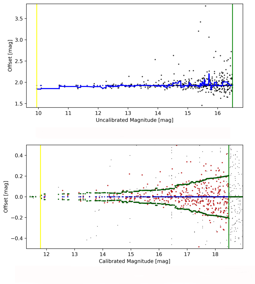
Figure 1: Example of the calibration of an image of IC 348 in a green (TG) filter into the V filter. Top panel: Difference ($m^{i}-m^{r}$) of the instrumental magnitudes between the TG image and the V-Band reference dataset. The blue line indicates the running median of the data-points and the two vertical lines indicate the range of instrumental magnitudes considered. Bottom panel: Difference ($m-m^{r}$) between the calibrated TG data and the V-Band reference frame. The larger (red) dots indicate stars with no problems in the photometry, while the remaining stars are shown as smaller (black) dots. The dotted (green) data points indicate the one sigma scatter for stars within 0.5 mag and the two vertical lines the range of magnitudes in which stars are included in the calibration.

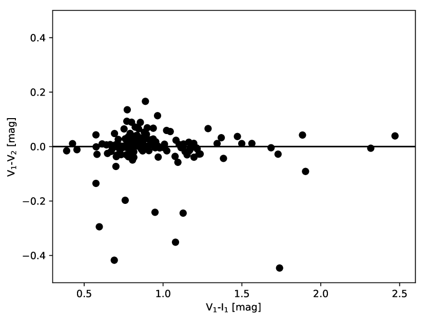
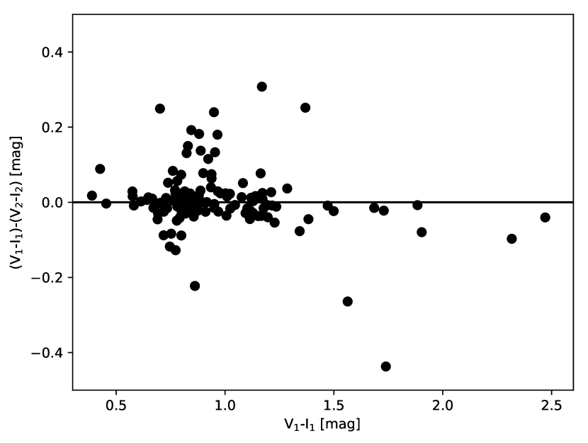
Figure 2: Differences of calibrated instrumental V-Band magnitudes and V-I colours for one of our targets. An index of 1 indicates data taken with the Beacon Observatory, while an index of 2 indicates data taken with the LCO. There are no significant and systematic trends of these differences with the V-I colour of the stars. Note that the V and I data for each telescope has been taken on the same night, but there is an observing time difference of several weeks between the two datasets, thus the outlier data-points represent variable stars.

Table 1: Properties of star forming regions and clusters investigated in this work. In the Table we list the following: name; position in RA/DEC (J2000) as used in the HOYS-CAPS project; total number of potential YSOs detected in at least 15 images; number of variable stars selected (total number, number of YSO candidates and number of other variable stars with high Stetson index); fraction of YSO candidates that are variable; fraction of variable objects that are classified as CTTSs (f${}^{\rm var}_{\rm CTTS}$) or transition/depletion disk objects (f${}^{\rm var}_{\rm WTTS}$); distance in [pc]; age in [Myr]; The references for distances and ages for the different regions are indicated in the name column and are from: ⁽¹⁾ Sicilia-Aguilar et al. (2005); ⁽²⁾ Contreras et al. (2002); ⁽³⁾ Bally et al. (2008); ⁽⁴⁾ Reipurth & Schneider (2008); ⁽⁵⁾ Guieu et al. (2009); ⁽⁶⁾ Harvey et al. (2008); ⁽⁷⁾ Scholz et al. (2013); ⁽⁸⁾ Román-Zúñiga & Lada (2008); ⁽⁹⁾ Dahm (2008); ⁽¹⁰⁾ Straižys et al. (2014). Typically the distance uncertainties are 10 – 20 %, but they are probably much higher for IC 5146.

Name	RA	DEC	Ntot	Nvar			f${}^{\rm YSO}_{\rm var}$	f${}^{\rm var}_{\rm CTTS}$	f${}^{\rm var}_{\rm WTTS}$	d	age
	(J2000)		YSO	tot	YSO	var	[$\%$]	[$\%$]	[$\%$]	[pc]	[Myr]
IC 1396 A(1,2)	21 36 35	+57 30 36	68	56	42	14	62	34	66	900	1 – 5
IC 348(3)	03 44 34	+32 09 48	88	37	36	1	41	49	51	300	2 – 4
IC 5070(4,5)	20 51 00	+44 22 00	152	107	105	2	69	87	13	600	3
IC 5146(6)	21 53 29	+47 16 01	166	67	58	9	35	57	43	950	1 – 5
NGC 1333(7)	03 29 02	+31 20 54	30	19	17	2	57	74	26	300	1 – 3
NGC2244(8)	06 31 55	+04 56 30	544	65	54	11	10	34	66	1400 – 1700	2 – 3
NGC2264(9)	06 40 58	+09 53 42	124	79	73	6	59	67	33	760	1 – 5
NGC 7129(10)	21 42 56	+66 06 12	35	36	28	8	80	39	61	1150	3

3 Data analysis

3.1 Selection of Young Clusters and their variable YSOs

For the analysis presented in this paper we selected the eight clusters/regions from the HOYS-CAPS target list which had the most observations available as of May 2017. These are: NGC 7129, IC 5070, NGC 2264, IC 1396 A, IC 348, NGC 1333, IC 5146 and NGC 2244. We present the basic data for these clusters (positions, distances, ages, number variable stars selected etc.) in Table 1.

In this paper we aim to generally characterise all variable YSOs in the above selected eight clusters. To achieve this we first cross-matched the optical photometry catalogues for our observed fields with catalogues of known and suspected members for each of the regions. In particular we used the following lists: Luhman et al. (2016) for NGC 1333 and IC 348; Dahm & Hillenbrand (2015) and Stelzer & Scholz (2009) for NGC 7129; Sicilia-Aguilar et al. (2005) for IC 1396 A; Dahm & Simon (2005) and Cody et al. (2014) for NGC 2264; Balog et al. (2007) for NGC 2244; Rebull et al. (2011) for IC 5070; and Harvey et al. (2008) for IC 5146. These catalogues are inhomogeneous in completeness, depth and selection criteria. In this work, they are only used to select variable young stars in these clusters which are detected in our optical data.

We then investigated the light-curves of all these YSO candidate members in each region. As we are trying to analyse the statistical behaviour of variable young stars, only objects which fulfilled the following criteria where selected for further analysis: i) There are more than 15 nights of data with photometry in V, R and I (or equivalent filter) taken in the same night; ii) The difference in magnitude between the brightest and faintest V-band measurement has to be larger than 0.2 mag (corresponding to about 5$\sigma$ for the brighter stars); iii) The Stetson index (Stetson, 1996) has to be larger than one. These criteria ensure that our sample is not significantly contaminated by non-variable stars with large photometric errors. The numbers of targets selected by our criteria in each region are listed in Table 1. In each cluster/region we analysed some additional objects which are not in one of the catalogues but fulfill the above criteria for variability. Their numbers are indicated separately in Table 1.

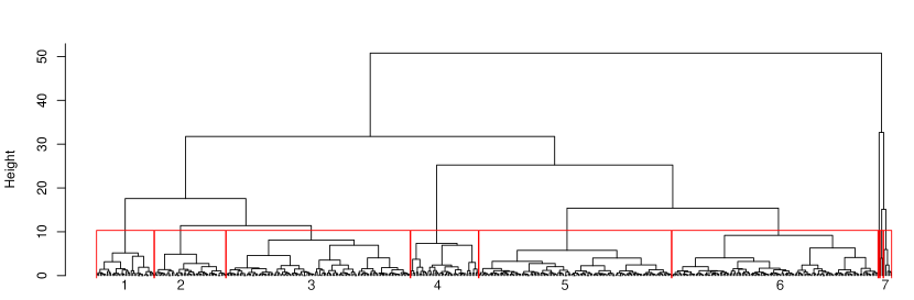
Figure 3: Resulting dendrogram of our hierarchical clustering analysis of the YSOs light-curves in our sample. The groups of YSOs identified are labeled at the bottom. All outliers on the right hand side of the dendrogram are combined into group 7. The main Table LABEL:yso_data_table in the Appendix lists the group number for each individual YSO.

3.2 Determination of light-curve properties

For each selected individual star we determined a number of light-curve properties from the available data. An example of some sets of light-curves can be found in Figs. 7, 8, and 9. These properties are the following:

• We fit a linear function (see Eq. 2) to the $N$ data-points in the V-I vs. V colour-magnitude diagram to determine the slope ($\alpha$) – indicated as green lines in the right hand side panels of Figs. 7, 8, and 9. This has been done by minimising the sum over all perpendicular distances of the data-points to the line of best fit (see Eq. 3) to ensure that for all extreme cases (colour independent magnitude changes and magnitude independent colour changes), the correct slope is determined. We determine the $rms$ value of all perpendicular distances to the line of best fit. We remove any outliers further than three times the $rms$ away from the line of best fit iteratively. These $rms$ values are almost exclusively larger than the photometric uncertainties of the individual data-points on both axes and thus only real outliers, such as in the case of V 350 Cep (Fig. 8) are removed. To ensure the procedure has worked for all objects, we manually inspected the graphs for all targets. For ease of presentation of the $\alpha$-values, we have converted them into degrees as otherwise some of the slopes have very large numerical values. Note that the photometric uncertainties of the data-points on both axes are correlated. This, however, has the effect of shifting data-points parallel to the $\alpha=45^{\circ}$ directions, and has thus no significant influence on the determined values.

  $$V=V_{0}+\alpha(V-I)$$ (2)

  $$\sum\limits^{N}_{i=1}\frac{\left|V_{0}(V-I)+\alpha-V\right|}{\sqrt{V_{0}^{2}+1}}$$ (3)

• After the calculation of the line of best fit and removal of outlying data-points, we determine the scatter ($rms$) of the data-points in the V-I vs V colour-magnitude diagram perpendicular to the line of best fit.

• Following Cody et al. (2014) we determine the asymmetry metric ($M$) for the V-Band light-curve using $M=\left(\left<d_{10\,\%}\right>-d_{\rm med}\right)/\sigma_{d}$, where $\left<d_{10\,\%}\right>$ is the mean of all magnitudes in the top and bottom ten percent of the V-Band light-curve, $d_{\rm med}$ the median of all magnitudes and $\sigma_{d}$ the overall rms of the V-Band data-points from the mean.

• Following Stetson (1996) we determine the Stetson index for the V-Band light-curve.

• We determine a cumulative distribution function (CDF) for the V-Band magnitudes after subtracting the median magnitude from each data-point.

We then use a two-sided, two sample Kolmogorov-Smirnov (KS) test to compare the CDFs of all objects against each other pairwise and record the KS statistics (D_KS) and resulting $p$-value. This value indicates the probability that the two samples (V-Band CDFs) are drawn from the same parent distribution. Hence, large $p$-values indicate pairs of stars with very similar distribution of V-Band magnitudes and vice versa.

3.3 YSO near and mid-IR SEDs

We have cross matched the objects investigated here with the WISE All-sky catalogue (Cutri & et al., 2013) and the 2MASS catalogue (Skrutskie et al., 2006). For some of our target regions there are Spitzer observations which are deeper than the WISE data. However, they are not available for all fields to a homogeneous depth, which we have for our optical data. Since more than 90 % of our objects have a WISE match in all four filters, we do not include the Spitzer data in our analysis. The WISE data has been used to determine the slope of the spectral energy distribution ($\alpha_{\rm SED}$) between 3.4 $\mu$m and 22 $\mu$m. Following Majaess (2013) we use:

$$\alpha_{\rm SED}=0.36\cdot(w1-w2)+0.58\cdot(w2-w3)+0.41\cdot(w3-w4)-2.90$$ (4)

Traditionally, objects with positive slopes $\alpha_{\rm SED}$ are classified as protostars, while negative slopes between $-2$ and zero indicate classical T-Tauri stars (CTTSs). Koenig & Leisawitz (2014) have presented a colour selection scheme in WISE to differentiate Class I protostars and Class II CTTSs based not just on $\alpha_{\rm SED}$ but considering all WISE colours (excluding the W4 magnitudes). There is no specific WISE colour selection for Weak-Line T-Tauri Stars (WTTS) as their colours overlap too much with normal stars as well as other objects such as AGB stars.

3.4 Hierarchical clustering of YSO light-curve properties

We aim to identify objects with similar light-curve properties automatically via a hierarchical clustering method. Here we briefly describe the methods involved. A more detailed discussion of them can be found in Campbell-White et al. (2018, subm.).

As a first step we establish a dissimilarity matrix which contains the pairwise distances ($d_{\rm(i,j)}$) between each pair of YSOs (i,j) for each of the properties. From the KS-test we already have $d^{\rm KS}_{\rm(i,j)}$ which is identical to the KS statistic D_KS. We also determine these distances for each of the other properties, i.e. $d^{\alpha}_{\rm(i,j)}=\left|\alpha_{\rm i}-\alpha_{\rm j}\right|$ for the slopes in the V-I vs V colour magnitude diagram; $d^{rms}_{\rm(i,j)}=\left|rms_{\rm i}-rms_{\rm j}\right|$ for the scatter of the data-points from the line of best fit in the same diagram, and $d^{M}_{\rm(i,j)}=\left|M_{\rm i}-M_{\rm j}\right|$ for the asymmetry metric of the V-Band light-curves.

To account for the different ranges in these four parameters, all the individual distances are normalised by the mean of all pairwise distances for the respective parameter. The final pairwise dissimilarity between two stars, considering all of the parameters is then calculated as:

$$d_{\rm(i,j)}=\sqrt{\left(\frac{d^{\rm KS}_{\rm(i,j)}}{\overline{d^{\rm KS}}}\right)^{2}+\left(\frac{d^{\alpha}_{\rm(i,j)}}{\overline{d^{\alpha}}}\right)^{2}+\left(\frac{d^{rms}_{\rm(i,j)}}{\overline{d^{rms}}}\right)^{2}+\left(\frac{d^{M}_{\rm(i,j)}}{\overline{d^{M}}}\right)^{2}}$$ (5)

An Euclidean distance matrix is then calculated from the $d_{\rm(i,j)}$-values (see Campbell-White et al. (2018, subm.) for details) and hierarchical clustering is performed on it to identify groups of YSOs with similar properties. Note that we will use ’groups’ throughout the paper when referring to these statistical associations, rather than ’cluster/region’ which refers to the investigated young clusters from which the YSOs are selected.

Groups are created from hierarchical clustering by considering, in the first instance, the distance between pairs of objects. Pairs with the smallest distances are joined, forming the first groups. Recursive merging then takes place, where at each stage, new inter-group distances are determined. The manner in which this happens depends on which hierarchical method is used. We have used Ward’s agglomerative method to form groups (Murtagh & Legendre, 2014), which seeks to minimise the distance between the centres of groups in Euclidean space, and has been shown to outperform other hierarchical methods (Ferreira & Hitchcock, 2009). Groups are iteratively formed until the final two groups merge. This process is represented by a dendrogram. Figure 3 shows all individual YSOs along the bottom, and groups are seen as the horizontal merges. The height on the dendrogram corresponds to the distance at which a merge was made, for pairs of YSOs, this was the Euclidean distance we have described, for all higher level groups, the height was taken from the value obtained with Ward’s method.

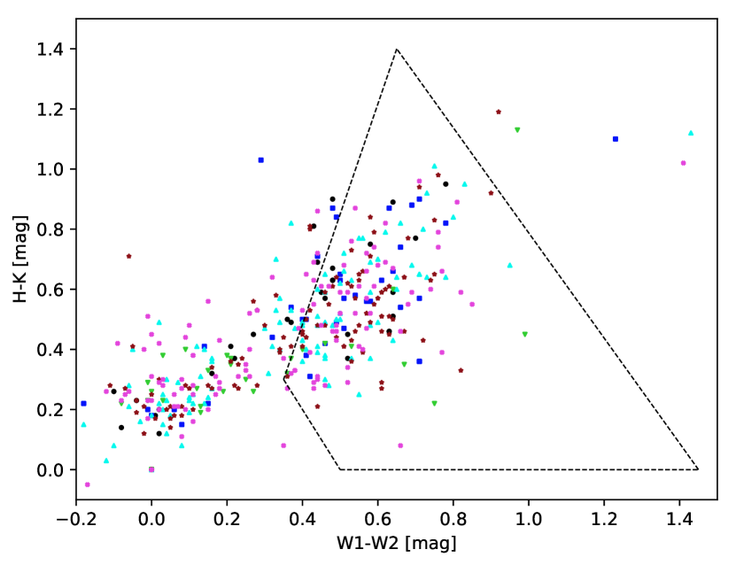
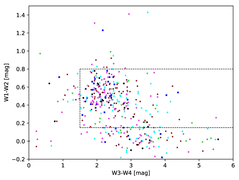
Figure 4: NIR/MIR colour-colour diagrams of the variable objects investigated. Left: WISE W1-W2 vs H-K 2MASS colour-colour plot. The dashed black lines enclose the region of CTTSs from Koenig & Leisawitz (2014). Class I protostars would be situated towards the top-right part of the diagram. Right: WISE W3-W4 vs W1-W2 diagram. The dashed black lines enclose the region for transition disks from Koenig & Leisawitz (2014). The two distinct groups of sources, separated by W1-W2 = 0.3 mag, can be clearly seen in both panels. The colours and symbols indicate membership in each of the groups identified with the hierarchical clustering: G 1 – black circles; G 2 – dark blue squares; G 3 – light blue triangles up; G 4 – green triangles down; G 5 – brown stars; G 6 – pink x’s; All outliers in G 7 are not shown.

4 Results and Discussion

4.1 Selection of variable YSOs

Our selection criteria for variable YSOs in the eight investigated regions have identified 466 objects which are included in the analysis in this paper. Of these, 413 (89 %) are included in one of the catalogues of potential cluster members, the remaining 53 objects (11 %) are included solely due to their variability. Hence, the sample of variables investigated will only contain a very small fraction of potentially non-YSO variables such as background giant stars. In Table 1 we detail the number of investigated variable stars in each of the clusters, split by their mode of selection. This table can be used as a compendium of variable YSOs in future studies, together with the main Table LABEL:yso_data_table in the Appendix where all individual stars and their properties are listed.

We estimate the fraction of variable stars (f${}^{\rm YSO}_{\rm var}$) amongst the detected YSOs. These fractions are also listed in Table 1. The mean fraction of variable stars is 52 % with a rms variation of 22 % between the individual regions. The highest fraction of variables (with 80 %) occurs in NGC 7129. In NGC 2244 the fraction is the lowest with only 10 % of the detected stars classified as variable. These numbers are only included here for completeness reasons, since (as indicated above) the strong variations in them are most likely a reflection of the our selection method and biases than that they are intrinsic to the properties of the regions (such as the age). Variability is expected to decline with the age of the region, and our ability to detect it will depend on the distance and extinction.

The colour-colour diagrams shown in Fig. 4 reveal that there are two distinct groups of objects in our sample of variable YSOs. The left panel of Fig. 4 shows the W1-W2 vs H-K diagram. It indicates the typical colours of CTTS from Koenig & Leisawitz (2014) and a large number of objects fall in or near the CTTS region. Note that protostars would be situated towards redder colours along both axes. A second group of objects with almost zero W1-W2 colour is also evident. The same two groups of objects can be identified in the right panel of Fig. 4 which shows the W3-W4 vs W1-W2 colour-colour diagram. One finds that the objects with low W1-W2 colours, falling below the marked box, show in part large W3-W4 values, thus indicating the presence of some cold disk material. These objects are thus most likely either transition disks with inner gaps or depleted disks.

Thus, for the purpose of this paper we characterise all sources with W1-W2 $>$ 0.3 mag as CTTS and all other sources as transition/depleted disks (referred to as WTTS, hereafter). Note that this criterion is only applicable as the vast majority of our sources are selected as known YSOs which are also variable, hence there is almost no contamination of non-YSOs in the sample. The fraction of CTTSs amongst the variables has been listed as f${}^{\rm var}_{\rm CTTS}$ in Table  1. The mean CTTS fraction in the full sample is 64 % (271 objects). The highest value in an individual region (87 %) is found in IC 5070 and the lowest (34 %) in IC 1396 A and NGC 2244. There are no apparent trends between these fractions and the age of the cluster/region they are in.

Table 2: Table with data of number/fraction of YSOs per region/cluster and group in dendrogram. We list the number ($N$) of objects in each of the groups from each young region/cluster. The first number in the brackets indicates what fraction $N$ represents in the region/cluster expressed in percent. The second number indicates what fraction $N$ represents in the group. For example for IC 5070 in G2 we find 13 (12,31), which means there are 13 objects in the region IC 5070 which are part of G 2 and these sources represent 12 % of all the objects in IC 5070 and 31 % of all the objects in G 2. The numbers in brackets in the ’Total’ row and column indicate the fraction of the total number of source in the sample. Note that due to rounding errors the fractions do not necessarily add up to 100 %.

Cluster	G1	G2	G3	G4	G5	G6	G7	Total
IC 1396 A	4 ( 7,12)	7 (13,17)	17 (30,16)	4 ( 7,10)	11 (20,10)	12 (21,10)	1 ( 2,13)	56 (12)
IC 348	0 ( 0, 0)	2 ( 5, 5)	6 (16, 6)	7 (19,18)	6 (16, 5)	14 (38,12)	2 ( 5,25)	37 ( 8)
IC 5070	4 ( 4,12)	13 (12,31)	20 (19,19)	5 ( 5,13)	40 (37,35)	25 (23,21)	0 ( 0, 0)	107 (23)
IC 5146	10 (15,29)	5 ( 7,12)	16 (24,15)	1 ( 1, 3)	18 (27,16)	17 (25,14)	0 ( 0, 0)	67 (14)
NGC 1333	3 (16, 9)	2 (11, 5)	4 (21, 4)	0 ( 0, 0)	2 (11, 2)	7 (37, 6)	1 ( 5,13)	19 ( 4)
NGC 2244	5 ( 8,15)	4 ( 6,10)	18 (28,17)	6 ( 9,15)	15 (23,13)	17 (26,14)	0 ( 0, 0)	65 (14)
NGC 2264	8 (10,24)	9 (11,21)	20 (25,19)	8 (10,20)	14 (18,12)	20 (25,17)	0 ( 0, 0)	79 (17)
NGC 7129	0 ( 0, 0)	0 ( 0, 0)	7 (19, 6)	9 (25,23)	7 (19, 6)	9 (25, 7)	4 (11,50)	36 ( 8)
Total	34 ( 7)	42 ( 9)	108 (23)	40 ( 9)	113 (24)	121 (26)	8 ( 2)	466

4.2 YSO groups from the Hierarchical Clustering

The hierarchical clustering results are presented in the dendrogram in Fig. 3. Usually the dendrogram is cut at a specific, albeit arbitrary, height to select groups of objects. We have chosen a value of 10 as the height at which the cut is made. This results in 6 clear groups (referred to as G hereafter) and some outliers. In Table LABEL:yso_data_table we list for each individual YSO which group it belongs to. One way of justifying the choice of the cut value is to read the dendrogram from the top down and to investigate if the identified groups share any physical properties.

The first branch that separates from the majority of objects is seen on the right hand side and contains 8 objects. These objects have basically no common properties with all of the remaining sources and are hence placed in G 7 (labeled in Fig. 3 together with all the other groups). The next separation in the dendrogram splits Gs 1, 2, 3 from Gs 4, 5, 6. As will be discussed later and indicated in Fig. 5, this splits the light-curves with dips from the light-curves which are symmetric or have outbursts.

The next split in the objects with dipper light-curve separates G 1 from the rest. According to Fig. 5, G 1 contains the most extreme dippers. The final split into G 2 and G 3 separates the objects with almost colour-independent dips (G 3) from the remaining dippers (G 2). Similarly, the first split of the burster light-curves separates the most extreme bursters (G 4) from the rest, which is then split into less extreme burster and symmetric light-curves (Gs 6, 5).

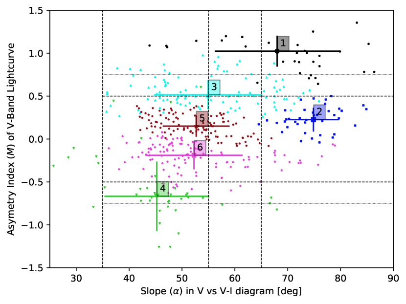
Figure 5: Figure showing the slope $\alpha$ in the V vs V-I diagram and the asymmetry index $M$ for the YSOs in our sample. The larger symbols and error bars indicate the mean and $rms$ of all stars in the different groups. The group number is also indicated. All outliers (summarised in G 7) are not shown as they are partly outside the parameter space of the plot (e.g. at negative slope values). The colours and symbols are the same as in Fig. 4. The dashed horizontal lines separate the dippers (top) from the symmetric light-curves (middle) and the bursters (bottom). The thin dashed horizontal lines separate the most extreme bursters and dippers. The dashed vertical lines indicate the three regions for $\alpha$ discussed in the text.

4.3 $\alpha$-values and $M$-values

In Fig. 5 we have plotted the positions of all variable objects (except the outliers in G 7) in the $\alpha$ – $M$ plane of the parameter space. Objects from the different groups are indicated by different colours and symbols. We also indicate the average values and $rms$ of all objects in each group. As one can see from this diagram and the discussion above, the hierarchical clustering seems to have separated the groups most clearly in this part of the parameter space. There is only minimal overlap between the groups with the exception of some scattered objects in G 4. The groups are (with the exception of G 2), separated by the asymmetry parameter $M$. Furthermore, the parameter space is not filled homogeneously. There are almost no sources with $\alpha$-values lower than 40^∘ and objects with negative $M$-values and high $\alpha$-values are extremely rare.

The value of the $\alpha$ parameter indicates the amount of colour change during brightness change. Objects with large values (close to 90^∘) basically do not change their colour at all. These objects can for example be eclipsing binaries where both components have similar colours. Changes in brightness due to variability in the amount of absorbing and scattering material along the line of sight (e.g. from the accretion disk) generally changes the colour in a determinable way. If the disk material is made from normal ISM dust then the $\alpha$-value should be between 60^∘ ($R_{V}=3.1$) and 66^∘ ($R_{V}=5.0$) if one uses a standard reddening law (Mathis, 1990). Higher values of $\alpha$ are possible if the obscuring material consists of larger dust grains than in the normal ISM or the objects undergo eclipse events by optically thick material.

Light-curves with $\alpha<55$^∘ are thus not consistent with variability due to changes in extinction alone. Objects that show $\alpha\approx 45$^∘ change their brightness in the V-Band but not at a detectable level in the I-Band. This can in principle be caused by non-variable red sources which are at the detection limit in V but detected at high signal-to-noise in the I-Band. However, our selection criteria for the variable sources will have removed these reliably. Alternatively, these objects can be interpreted as sources with large fluctuations at visual wavelengths and small, undetected variations in the infrared. Hence, the most likely cause for the variability in objects with $\alpha<55$^∘ is changes in the accretion rate or the properties of large hot/cold spots. Thus, based on the $\alpha$-value we can classify the sources in the following three categories:

• 65^∘$\leq\alpha\leq 90$^∘: Light-curves consistent with variable extinction due to larger grains or eclipses by optically thick material

• 55^∘$\leq\alpha\leq 65$^∘: Light-curves consistent with variable extinction due to normal ISM dust grains

• 35^∘$\leq\alpha\leq 55$^∘: Light-curves not consistent with variable extinction, thus most likely caused by changes in accretion rates or hot/cold surface spots

Naturally there will be sources whose properties are a mix of more than one of these physical reasons for variability. Hence these categories will only be indicative of what the main reason for the variability in a group of objects might be if it falls within one of the specified regions for the $\alpha$-values. In total there are 252 objects whose $\alpha$-value is in agreement of their variability being dominated by accretion rate changes or spots. In the group that is dominated by variable ISM extinction there are 94 sources, and in the group of objects which are most likely due to variable extinction by larger grains or eclipses we have 108 sources. The remaining objects fall outside this part of the parameter space.

We can also split the sample of sources according to the asymmetry metric $M$. As detailed in Cody et al. (2014) objects with negative values are bursters, i.e. objects that show short duration increases in brightness compared to their normal magnitudes. On the other hand, objects with positive values for $M$ are dippers, which have short duration decreases in brightness compared to normal. Cody et al. (2014) use $\pm 0.25$ as thresholds for $M$ to identify bursters and dippers. Here we employ a slightly more conservative value and will identify an object as burster if $M<-0.5$, while objects with $M>0.5$ are considered dippers. Objects with $M$-values in-between these borders are considered to have a symmetric behaviour. In total our sample contains 41 bursters, 101 dippers and 324 symmetric variables. If we use an even more conservative threshold of $M\pm 0.75$ to select the most extreme bursters and dippers we find 10 and 51, respectively.

From this discussion and from Fig. 5 it is clear that our objects do not fill the parameter space homogeneously. In particular there is not a single object whose properties are in agreement with variability due to eclipse events ($\alpha$ near 90^∘), which at the same time belongs into the burster group. This is understandable, since almost all eclipsing binary objects spend most of their time outside the eclipse state and eclipsing binaries that also show outbursts might be characterised as having a ’symmetric’ light-curve.

As already briefly discussed in Sect. 4.2 the groups of YSOs generated by the hierarchical clustering, do not have a simple one-to-one matching with any one of the physical characteristics, but there are clear trends. Most of the objects in G 4 fall into the burster category and most of them also are in agreement with having variable accretion rates or spots. Indeed more than 50 % of the G 4 members are in the accretion burst/spot category. Similarly, members in G 1 are almost exclusively in agreement with dipper light-curves, most of them in the extreme category. Most of the light-curves in G 1 are either in agreement with variable extinction or eclipses, only four sources fall into the variable accretion rate/spot category. All the sources in G 2 fall into the eclipse category, and all of the light-curves are symmetric. The objects sorted into the other groups (G 3, 5, 6) are all a mix of accretion/spot and extinction variability, where G 3 contains objects with slightly dipping light-curves. G 5/G 6 contain symmetric light-curves with slightly positive $M$-values in G 5 and negative ones in G 6.

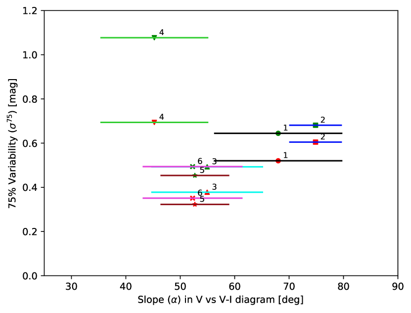
Figure 6: Figures showing the 75 % variability ($\sigma^{75}$) in V and R for the groups identified with the hierarchical clustering. The green symbols indicate $\sigma^{75}_{V}$ and the red symbols $\sigma^{75}_{R}$. The symbol types, numbers and colour of the lines are the same as in Fig. 4.

4.4 Variability

We determine the typical variability in the V-Band and R-Band for groups of YSOs identified in the hierarchical clustering. This utilises the total CDF for all magnitudes determined as the average of all individual CDFs of all stars in each group. We then determine the magnitude range around the median value within which 75 % of the brightness measurements are situated and refer to this from here on as 75 % variability or $\sigma^{75}$.

In Fig. 6 we show $\sigma^{75}$ of all groups in the V and R-Band plotted against the average $\alpha$-value. In all cases, $\sigma^{75}_{V}$ is larger than $\sigma^{75}_{R}$ by at least about 0.1 mag. The lowest variability (about 0.5 mag in V and 0.4 mag in R) is measured for Gs 3, 5, 6 which represent the symmetric light-curves. Slightly higher variability (0.7 mag in V and 0.6 mag in R) is found for Gs 1, 2. These are all objects whose light-curves can be characterised as dippers and all of them are also in agreement with variable extinction or eclipse behaviour.

The most variable sources (about 1.1 mag in V and 0.7 mag in R) are the objects in G 4, i.e. the objects most likely in agreement with outbursts due to variable accretion rates (the magnitudes of the variability in this group exclude spots as causes in most cases). Objects in this group also show the largest difference $\sigma^{75}_{V}-\sigma^{75}_{R}$. While for all other groups there is only a 0.1 mag difference between the V and R filters, for G 4 the difference is 0.4 mag. This can only in part be explained by the low $\alpha$-values of the sources, as especially Gs 5, 6 have similar values, but the difference in variability from R and V is much smaller, both in absolute and relative terms.

4.5 YSO properties in Clusters/SF Regions

In Table 2 we have indicated for each group from the hierarchical clustering the number of members and how they are distributed amongst the investigated young clusters and SF regions. We find that there are three groups (Gs 2, 5, 6) which roughly contain one quarter of all the sources each. The remaining three groups (Gs 1, 2, 4) each roughly contain 10 % of all the objects. The fraction of sources considered outliers (summarised in G 7) is extremely small with less than 2 % but this group naturally contains the most unusual objects in the sample.

We have checked if any cluster or SF region has an abnormally high/low representation of objects in a particular group. There are a two notable cases: i) A quarter of all objects from NGC 7129 are in G 4, while this group only contains 9 % of all objects; ii) Half of all objects in G 7 are from NGC 7129, while this region/cluster only represents 8 % of all objects. Thus, NGC 7129 seems to be unusual in that it contains a larger fraction of YSOs whose light-curves can be characterised as bursters caused by accretion rate variations. The cluster also seems to contain a high fraction of objects with unusual light-curves. However, small number statistics as well as selection biases could be responsible for these abnormalities.

An investigation into potential differences in the light-curve properties of CTTSs and WTTSs in our sample has not led to any significant results. There are hints that the fraction of objects whose light-curves can be interpreted as being caused by occultations by material made up of larger dust grains is increased amongst the WTTS population. This is not statistically significant, however it does warrant a more detailed investigation in future.

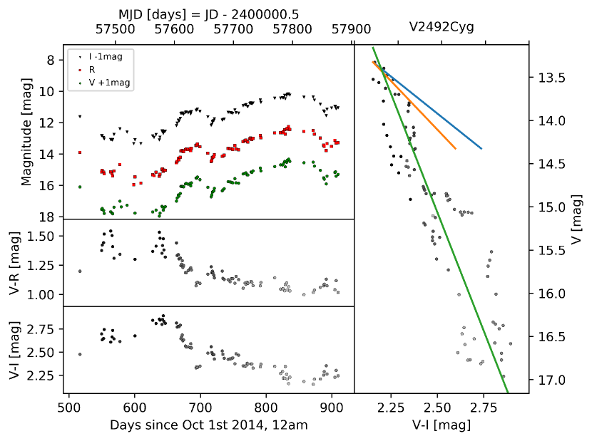
Figure 7: Light-curve of the star V 2492 Cyg. In the top left panel we show the instrumental magnitudes (shifted to approximately correspond to the apparent magnitude) for the V, R and I filters. Note that images taken in a different filter have been calibrated into the VRI system. The two panels in the bottom left show the evolution of V-R and V-I colour of the source. The colour of the data-points represents the V-Band magnitude. Black symbols correspond to the faintest magnitudes and light-gray symbols to brighter magnitudes. The right panel shows the position of all observations in the V-I vs V colour-magnitude diagram. Here the colour of the symbols corresponds to the time of the observations. The darkest points correspond to the most recent data. The green line is the line of the best linear fit to the data after removing outliers. The red and blue line indicate extinction vectors for $A_{V}=1$ mag for $R_{V}=3.1$ (blue) and $R_{V}=5.0$ (red).

4.6 Discussion of selected individual Sources

In this section we discuss three selected objects – V 2492 Cyg, V 350 Cep, 2MASS J21383981$+$5708470 in more detail. The determined properties for all individual sources are listed in Table LABEL:yso_data_table in the Appendix.

4.6.1 V 2492 Cyg in IC 5070

The light-curve of V 2492 Cyg is shown in Fig. 7. The source is also known as IRAS 20496$+$4354, WISE J205126.22$+$440523.8 or PTF 10 nvg. On 2016-02-22 it was also published as Gaia 16 aft. In Table LABEL:yso_data_table the source is called R11 T1 205126.22$+$440523.7, as this is the designation in the YSO list from Rebull et al. (2011), which we used to select objects in IC 5070.

The object has been studied by numerous authors in the past, e.g. Kun et al. (2011); Aspin (2011); Covey et al. (2011); Kóspál et al. (2011); Hillenbrand et al. (2013); Kóspál et al. (2013); Scholz et al. (2013); Giannini et al. (2017). It also was subject of many Astronomer’s Telegrams, e.g. Arkharov et al. (2015); Munari et al. (2017); Ibryamov & Semkov (2017); Froebrich et al. (2017). The object is considered an embedded Class I protostar that shows stochastic high amplitude variations in brightness. This variability is driven by changes in accretion rate as well as extinction (up to $\Delta A_{V}$ = 30 mag), i.e. restructuring of the inner disk. Near infrared spectra are similar to McNeil’s Nebula (V 1647 Ori) and the source might be considered as a young, embedded analogue to UX Ori type stars. Typical variations in brightness occur over timescales of months to years, with a $\sim$220 day quasi-periodic signal reported in Hillenbrand et al. (2013).

All of the data in our light-curve has been included in Froebrich et al. (2017). There is no indication of the 220 day quasi-periodic signal identified in Hillenbrand et al. (2013). Instead, after a minimum brightness between April and July 2016, the object has steadily increased its brightness to a maximum at the end of January 2017. The object then declined in brightness and the total variations observed in our data are $\Delta$V $\approx$ 4 mag. The colour-magnitude diagram indicates that the variations are consistent with changing extinction from larger dust grains. However, there are large and systematic deviations from this simplistic picture, which indicate changes in accretion rate as well as changes in the properties of the occulting material.

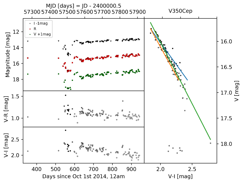
Figure 8: As Fig. 7 but for the object V 350 Cep

4.6.2 V 350 Cep in NGC 7129

We show the light-curve of V 350 Cep in Fig. 8. The source is also known as 2MASS J21430000$+$6611279, NGC 7129 IRS 1 or NGC 7129 FIR 3. In Table LABEL:yso_data_table the source is called HBC$\_$732, as this is the designation in the YSO list from Stelzer & Scholz (2009), which we used to select objects in NGC 7129.

The long term light-curve of this object (Ibryamov et al., 2014) shows an about 5 mag increase in the Blue/pg magnitude between 1965 and 1975, and the source has remained at this level since with typical variations of about 0.5 mag. The data presented in Ibryamov et al. (2014) suggest a ’dip’ of up to 1 mag in V for several months during 2009. The source has been interpreted as both FU-Ori and EX-Lup (EX-Or) candidate by several authors (Dahm & Hillenbrand, 2015; Magakian et al., 1999; Miranda et al., 1994). Typical FU-Ori spectral features are missing while EX-Or features are present, however the duration of the burst of now approximately 45 yrs seems atypical for an EX-Or.

On 2016-04-23 the object was reported as Gaia 16 alt. It showed two Gaia data-points clearly below its usual brightness. This event was also reported by Semkov et al. (2017) who covered the occultation event with 7 BVRI data-points. Our light-curve in Fig. 8 shows the event at an even higher time resolution. In total 13 VRI measurements are taken during the occultation event. When combining our data with Semkov et al. (2017) we find that the object has been detected in occultation between 2016-04-12 and 2016-05-25. Considering the closest data-points outside the occultation we estimate a duration of 51 – 83 days for the event. The light-curve shows that there are at least two ’dips’ with an intermittent maximum on 2016-04-17.

After the occultation the object returned to maximum brightness, just to drop again by about 0.5 mag in V, from which it has then recovered steadily. We find the depth of the minimum to be $\Delta$V = 2.05 mag, $\Delta$R = 1.80 mag and $\Delta$I = 1.90 mag. These are slightly deeper than reported in Semkov et al. (2017). The colour-magnitude plot shows that the first magnitude of decrease during the occultation, as well as the steady recovery of the flux after it, are in good agreement with a variation caused by changes in extinction due to normal ISM dust grains. During the deeper part of the occultation, the change in brightness turns completely free of colour change. Hence, the denser part of the occulting material responsible for this seems to have consisted of larger dust grains or the obscuring material was optically thick.

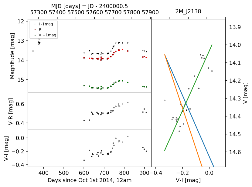
Figure 9: As Fig. 7 but for the object 2MASS J21383981$+$5708470

4.6.3 2MASS J21383981$+$5708470 in IC 1396 A

The light-curve of the source 2MASS J21383981$+$5708470, also known as $[$NSW2012$]$ 284 is shown in Fig. 9. This star is listed as Emission Line star in SIMBAD and has been identified in Nakano et al. (2012). In Table LABEL:yso_data_table the source is called Variable$\_$V$\_$324.665863$\_$57.146301, as it was added as a variable source due to its large Stetson index in the V-Band and was not included in the YSO candidate list from Sicilia-Aguilar et al. (2005), which we used to select objects in IC 1396 A.

The object shows a smooth brightness increase over about 150 days in all three filters. At the peak the brightness increase in V is about 0.4 mag, while in the I-Band the star got about 0.6 mag brighter. The Stetson index of the source is 1.36 and the asymmetry index -0.74, i.e. the object is classified as burster. What is highly unusual about this source is the change in colour towards red during the outburst. The angle in the V vs. V-I diagram is -59^∘. This is the only source in the entire sample with such a behaviour and consequently the object has been made part of the outlier group G 7 by the hierarchical clustering algorithm. The older I-Band (only) data suggests that there might have been another such burst about 600 days prior to the one covered by our survey. But only a small part of this potential burst is covered. If this is a periodic behaviour, then the next burst should occur at about MJD = 58300 d – which is early 2018. The nature of this source is unclear. Usually objects in outburst are bluer in the bright state. Hence, the object has either an unusual burst, or we see only scattered light from this source.

5 Conclusions

We are describing and presenting the first results of our optical survey of nearby clusters and star forming regions with small telescopes. All observations are obtained with the University of Kent’s 17″ Beacon Observatory or as part of the HOYS-CAPS citizen science project. In this paper we present the analysis of variable stars in eight target fields for which V, R and I-Band data has been taken over a period of about two years.

In our dataset we have identified 466 variable stars, 413 of which are confirmed YSOs, based on the Stetson index of their light-curves. For all objects light-curve properties such as the the asymmetry metric and slope ($\alpha$) in the V-I vs. V colour-magnitude diagram are determined. This sample is one of the largest samples of variable YSOs in the northern hemisphere with multi colour observations of such a time span and cadence, with additional archival multi-wavelength data and which is well suited for follow up observations. We find that the number of protostars in our sample is negligible, while about 65 % of the objects are CTTSs and about 35 % are sources with transition or depleted disks.

A detailed investigation of the asymmetry index $M$ and the $\alpha$-values of the light-curves has been performed. We can use the $\alpha$-value to characterise the most likely mechanism responsible for the variability in the stars. These range from occultations by material composed of large dust grains or optically thick material (including eclipses) to occultations by material consistent with normal ISM dust to changes in mass accretion rates or dark/bright spots. Dipper light-curves consistent with changes in accretion rates or spots are rare, there are virtually no burster objects that are consistent with occultations or eclipses. Burster light-curves also show by far the highest variability (of the order of 1.1 mag in V), followed by dippers and eclipsing objects (0.7 mag), and the symmetric light-curves have the lowest variations (0.5 mag).

We used a hierarchical clustering algorithm to identify groups of YSOs with similar light-curve properties. This clustering algorithm allows us to identify the most unusual objects in our sample. We further find that clustering results in groups of YSOs that correspond to dippers, bursters or symmetric light-curves and they also have different $\alpha$-values. Thus, grouping variable YSOs via hierarchical clustering using their light-curve properties is a promising approach for future studies of larger samples of YSOs that will become available e.g. from GAIA or the LSST.

Appendix A Data of Individual Sources

Table 3: This table lists the individual properties of all stars investigated in the papers. We list the catalogue name of the source, the name of the cluster/region it is in, the Right Ascention and Declination (J2000), the number of points in the lightcurve used to determine the slope $\alpha$ in the V vs V-I diagram, the slope $\alpha$ of a linear fit in the V vs V-I; the $rms$ of the datapoints from the fit, the Asymmetry index $M$, the Stetson index $S$, the group in the dendrogram the source is associated with, the range of magnitudes and the $rms$ of the V, R and I-Band lightcurve.

Source Name	Region	RA	DEC	Nvar	$\alpha$	$rms$	$M$	$S$	G	$\Delta{\rm V}$	$\sigma_{\rm V}$	$\Delta{\rm R}$	$\sigma_{\rm R}$	$\Delta{\rm I}$	$\sigma_{\rm I}$
		(J2000) [deg]			[deg]	[mag]				[mag]	[mag]	[mag]	[mag]	[mag]	[mag]
2MASS$\_$J03281101$+$3117292	NGC1333	52.045917	31.29147	19	44.0	0.013	-0.24	1.72	6	0.80	0.19	0.14	0.04	0.05	0.02
2MASS$\_$J03283692$+$3117353	NGC1333	52.153833	31.29317	18	45.4	0.047	0.04	2.09	6	0.96	0.24	0.31	0.08	0.24	0.06
2MASS$\_$J03283692$+$3117353	NGC1333	52.153833	31.29317	19	46.0	0.046	0.28	1.66	5	0.60	0.18	0.32	0.07	0.24	0.06
2MASS$\_$J03285101$+$3118184	NGC1333	52.212542	31.30514	23	72.1	0.101	0.90	2.33	1	1.21	0.26	1.06	0.23	1.28	0.26
2MASS$\_$J03285216$+$3122453	NGC1333	52.217333	31.37925	24	71.3	0.048	0.91	2.37	1	0.79	0.22	0.73	0.20	0.57	0.16
2MASS$\_$J03285741$+$3119505	NGC1333	52.239208	31.33072	17	46.6	0.021	0.87	1.02	3	0.71	0.15	0.23	0.06	0.13	0.03
2MASS$\_$J03285954$+$3121467	NGC1333	52.248125	31.36300	23	78.5	0.107	-0.06	6.62	6	3.09	0.75	2.74	0.66	2.49	0.62
2MASS$\_$J03290386$+$3121487	NGC1333	52.266083	31.36353	25	50.7	0.085	0.39	1.23	3	0.55	0.14	0.53	0.15	0.44	0.12
2MASS$\_$J03291037$+$3121591	NGC1333	52.293250	31.36644	25	58.7	0.139	0.32	4.28	3	1.41	0.42	0.99	0.30	1.04	0.28
2MASS$\_$J03292187$+$3115363	NGC1333	52.341125	31.26008	23	77.1	0.062	0.41	7.48	2	3.34	0.84	2.72	0.66	2.86	0.68
2MASS$\_$J03292204$+$3124153	NGC1333	52.341833	31.40428	24	51.2	0.149	-0.07	6.41	6	2.66	0.71	1.79	0.52	0.95	0.23
2MASS$\_$J03292591$+$3126401	NGC1333	52.358000	31.44447	24	-89.9	0.041	0.50	2.63	7	1.33	0.30	1.40	0.32	1.39	0.31
2MASS$\_$J03292889$+$3058418	NGC1333	52.370375	30.97828	20	51.7	0.089	-0.15	1.63	6	0.66	0.17	0.40	0.11	0.39	0.12
2MASS$\_$J03292925$+$3118347	NGC1333	52.371917	31.30967	19	45.8	0.025	0.48	1.12	3	0.61	0.14	0.14	0.05	0.12	0.03
2MASS$\_$J03294592$+$3104406N	NGC1333	52.441208	31.07811	16	48.9	0.018	-0.53	1.06	6	0.50	0.13	0.19	0.05	0.10	0.03
2MASS$\_$J03294592$+$3104406S	NGC1333	52.441750	31.07750	19	49.1	0.022	-0.55	1.31	6	0.50	0.13	0.22	0.06	0.12	0.03
2MASS$\_$J03295403$+$3120529	NGC1333	52.475125	31.34806	23	56.4	0.049	0.03	2.37	5	0.80	0.21	0.54	0.16	0.27	0.08
Variable$\_$R$\_$52.557724$\_$31.280481	NGC1333	52.557721	31.28048	24	83.1	0.037	1.36	1.07	1	0.59	0.14	0.45	0.13	0.48	0.13
Variable$\_$R$\_$52.647858$\_$31.266247	NGC1333	52.647854	31.26624	17	79.7	0.090	0.35	2.66	2	0.96	0.27	0.93	0.21	0.81	0.24
Cl$\_$NGC$\_$7129$\_$EGM$\_$8	NGC7129	325.635000	66.08308	41	35.7	0.100	0.32	1.71	3	0.73	0.18	0.49	0.12	0.48	0.11
SS2009$\_$NGC$\_$7129$-$S3$-$X41	NGC7129	325.662125	66.11908	76	48.1	0.101	-0.04	5.22	6	2.15	0.54	3.41	0.70	0.89	0.15
2MASS$\_$J21424023$+$6613287	NGC7129	325.667625	66.22464	18	69.4	0.182	-0.19	3.02	6	1.02	0.29	1.10	0.31	1.25	0.33
2MASS$\_$J21424608$+$6605562	NGC7129	325.692000	66.09894	29	43.7	0.064	-0.15	2.08	6	1.59	0.29	0.92	0.17	0.60	0.10
2MASS$\_$J21424613$+$6613460	NGC7129	325.692167	66.22939	22	43.3	0.071	0.12	1.70	5	0.59	0.17	0.47	0.13	0.34	0.08
2MASS$\_$J21424687$+$6606574	NGC7129	325.695292	66.11594	26	47.9	0.367	0.43	10.94	4	4.44	1.21	4.26	1.15	2.27	0.51
2MASS$\_$J21424705$+$6604578	NGC7129	325.696042	66.08272	108	56.3	0.054	0.09	1.43	5	1.01	0.16	0.72	0.11	0.58	0.09
2MASS$\_$J21424790$+$6606530	NGC7129	325.699583	66.11472	63	42.3	0.342	0.01	12.11	4	4.08	1.22	2.82	0.89	1.76	0.43
2MASS$\_$J21425092$+$6606036	NGC7129	325.712167	66.10100	68	44.2	0.218	-0.68	5.94	4	4.10	0.72	4.16	0.60	1.31	0.28
2MASS$\_$J21425234$+$6605350	NGC7129	325.717917	66.09314	39	44.9	0.343	-0.43	12.92	4	3.99	1.28	4.65	1.39	1.87	0.44
MMN2004b$\_$$\_$6	NGC7129	325.719208	66.11589	40	34.6	0.964	0.25	11.56	7	5.37	1.27	3.01	0.74	3.24	1.05
2MASS$\_$J21425321$+$6607207	NGC7129	325.721708	66.12244	67	16.6	2.392	0.86	8.86	7	4.13	0.98	2.73	0.55	4.88	1.42
MMN2004b$\_$$\_$9	NGC7129	325.722875	66.13481	88	47.9	0.128	-0.65	4.51	4	3.55	0.51	2.58	0.56	0.95	0.19
MMN2004b$\_$11	NGC7129	325.734375	66.10058	98	45.1	0.092	0.20	3.71	5	2.51	0.41	0.95	0.17	0.72	0.12
2MASS$\_$J21425719$+$6606346	NGC7129	325.738125	66.10969	100	48.7	0.178	-0.58	5.89	4	3.83	0.70	2.25	0.44	1.37	0.26
2MASS$\_$J21425836$+$6605273	NGC7129	325.743167	66.09092	31	23.1	0.636	0.79	4.58	7	1.98	0.50	1.50	0.44	2.33	0.55
SS2009$\_$NGC$\_$7129$-$S3$-$X17	NGC7129	325.744875	66.11022	66	43.4	0.390	-0.57	8.72	4	4.18	0.97	3.01	0.57	2.36	0.48
HBC$\_$731	NGC7129	325.748375	66.07606	29	48.0	0.115	-0.50	3.93	6	2.09	0.45	3.06	0.80	0.74	0.16
2MASS$\_$J21425997$+$6601010	NGC7129	325.749875	66.01694	18	42.7	0.062	-0.35	1.57	6	0.62	0.16	0.34	0.09	0.36	0.08
HBC$\_$732	NGC7129	325.750000	66.19108	93	67.4	0.065	0.88	4.21	3	2.43	0.54	2.25	0.49	2.13	0.45
2MASS$\_$J21430188$+$6606447	NGC7129	325.757833	66.11242	95	50.8	0.267	-0.65	4.92	4	3.52	0.61	2.91	0.51	1.92	0.36
2MASS$\_$J21430343$+$6605264	NGC7129	325.764292	66.09067	83	47.7	0.636	0.92	10.60	7	4.33	1.14	2.79	0.58	3.11	0.76
EM$\_$LkHA$\_$$\_$234	NGC7129	325.778417	66.11506	69	63.1	0.052	0.76	1.23	3	0.90	0.17	0.84	0.14	0.69	0.13
2MASS$\_$J21431141$+$6612555	NGC7129	325.797542	66.21542	62	52.0	0.073	0.07	2.17	5	1.06	0.23	0.79	0.16	0.62	0.12
MMN2004b$\_$19	NGC7129	325.820125	66.09683	56	43.7	0.069	0.28	2.01	5	1.07	0.21	0.69	0.12	0.42	0.09
MMN2004b$\_$20	NGC7129	325.882583	66.14739	64	50.7	0.077	0.57	2.20	3	0.92	0.21	1.05	0.15	0.93	0.14
MMN2004b$\_$22	NGC7129	325.931000	66.12522	57	44.9	0.051	0.14	1.53	5	0.78	0.17	0.44	0.10	0.26	0.06
2MASS$\_$J21440634$+$6604231	NGC7129	326.026417	66.07308	29	72.1	0.104	-0.28	4.35	6	1.56	0.42	1.22	0.37	1.02	0.32
Variable$\_$V$\_$325.765320$\_$65.914452	NGC7129	325.765292	65.91444	87	49.2	0.069	-0.40	1.33	6	0.80	0.15	0.45	0.10	0.47	0.10
Variable$\_$V$\_$326.092896$\_$65.714478	NGC7129	326.092875	65.71447	75	25.7	0.146	-0.31	1.01	4	2.55	0.25	0.39	0.07	0.62	0.12
Variable$\_$R$\_$325.348419$\_$65.927155	NGC7129	325.348417	65.92714	115	65.7	0.036	0.29	3.46	3	1.52	0.36	1.28	0.30	0.83	0.20
Variable$\_$R$\_$326.391418$\_$66.144142	NGC7129	326.391417	66.14414	99	64.7	0.049	-0.05	1.75	5	0.82	0.17	0.64	0.14	0.48	0.11
Variable$\_$R$\_$325.269501$\_$65.916420	NGC7129	325.269500	65.91642	72	43.8	0.101	-0.19	1.65	6	0.78	0.18	0.71	0.15	0.75	0.13
Variable$\_$R$\_$324.865295$\_$65.864845	NGC7129	324.865292	65.86483	62	38.1	0.132	-0.35	1.39	6	0.93	0.16	0.85	0.19	0.82	0.16
Variable$\_$I$\_$325.387939$\_$66.372276	NGC7129	325.387917	66.37225	101	74.1	0.026	0.57	2.30	3	1.22	0.25	1.01	0.21	0.84	0.17
Variable$\_$I$\_$325.059357$\_$66.457283	NGC7129	325.059333	66.45728	98	66.0	0.059	0.72	1.92	3	1.36	0.21	1.23	0.18	1.11	0.17
2MASS$\_$J21351745$+$5748223	IC1396A	323.822708	57.80619	17	44.9	0.046	-0.10	1.23	6	0.50	0.14	0.34	0.08	0.22	0.06
2MASS$\_$J21351861$+$5734092	IC1396A	323.827542	57.56922	22	65.5	0.035	0.56	1.34	3	0.60	0.15	0.39	0.12	0.36	0.10
2MASS$\_$J21353021$+$5731164	IC1396A	323.875875	57.52122	23	46.9	0.052	0.01	1.32	5	0.50	0.14	0.29	0.09	0.26	0.07
2MASS$\_$J21364941$+$5731220	IC1396A	324.205875	57.52278	26	52.7	0.067	-0.39	1.69	6	0.62	0.17	1.10	0.33	0.35	0.09
2MASS$\_$J21365579$+$5736533	IC1396A	324.232458	57.61481	19	46.1	0.045	0.51	1.11	3	0.43	0.13	0.17	0.05	0.26	0.06
2MASS$\_$J21365767$+$5727331	IC1396A	324.240292	57.45919	23	72.5	0.062	-0.28	3.25	6	1.51	0.34	1.15	0.30	0.91	0.23
2MASS$\_$J21370088$+$5725224	IC1396A	324.253667	57.42289	19	50.8	0.092	0.50	1.70	3	0.77	0.17	0.64	0.15	0.77	0.15
2MASS$\_$J21371031$+$5730189	IC1396A	324.292958	57.50525	16	51.0	0.049	-0.63	1.07	4	0.43	0.12	0.40	0.11	0.24	0.06
2MASS$\_$J21371054$+$5731124	IC1396A	324.293917	57.52011	25	56.6	0.067	0.27	1.24	5	0.46	0.13	0.31	0.09	0.41	0.10
2MASS$\_$J21371183$+$5724486	IC1396A	324.299292	57.41350	20	52.7	0.048	0.09	1.05	5	0.46	0.12	0.29	0.08	0.26	0.07
2MASS$\_$J21371215$+$5727262	IC1396A	324.300625	57.45728	19	62.0	0.058	1.08	1.40	1	0.63	0.17	0.40	0.10	0.42	0.11
2MASS$\_$J21371591$+$5726591	IC1396A	324.316292	57.44975	25	66.4	0.045	1.12	2.44	1	1.42	0.33	1.07	0.25	0.96	0.21
2MASS$\_$J21373420$+$5726154	IC1396A	324.392500	57.43761	18	46.8	0.060	0.62	1.33	3	0.47	0.13	0.24	0.07	0.35	0.09
2MASS$\_$J21374486$+$5724135	IC1396A	324.436917	57.40375	22	71.4	0.071	0.20	2.04	2	0.70	0.19	0.56	0.17	0.58	0.15
2MASS$\_$J21374514$+$5719423	IC1396A	324.438083	57.32842	19	62.0	0.086	-0.33	2.07	6	0.82	0.21	0.60	0.18	0.70	0.17
2MASS$\_$J21375018$+$5733404	IC1396A	324.459083	57.56122	23	69.3	0.050	0.47	1.53	3	0.63	0.15	0.48	0.13	0.46	0.11
2MASS$\_$J21375022$+$5725487	IC1396A	324.459250	57.43019	23	54.0	0.074	-0.17	1.23	6	0.55	0.14	0.47	0.11	0.42	0.10
2MASS$\_$J21375107$+$5727502	IC1396A	324.462792	57.46394	20	52.5	0.065	0.50	1.08	3	0.69	0.14	0.39	0.10	0.42	0.10
2MASS$\_$J21375812$+$5731199	IC1396A	324.492167	57.52219	24	62.6	0.039	-0.21	2.04	6	0.57	0.18	0.39	0.14	0.29	0.10
2MASS$\_$J21375841$+$5718046	IC1396A	324.493375	57.30128	19	48.8	0.088	0.31	1.22	5	0.64	0.14	0.57	0.12	0.51	0.13
2MASS$\_$J21380350$+$5741349	IC1396A	324.514583	57.69303	25	78.2	0.045	0.50	3.77	2	1.52	0.39	1.27	0.34	1.18	0.30
2MASS$\_$J21381731$+$5731220	IC1396A	324.572125	57.52278	24	69.5	0.029	0.33	2.90	2	1.14	0.28	0.92	0.23	0.77	0.19
2MASS$\_$J21381749$+$5741019	IC1396A	324.572875	57.68386	16	50.9	0.087	-0.18	1.67	6	0.72	0.18	0.48	0.12	0.51	0.12
2MASS$\_$J21382596$+$5734093	IC1396A	324.608167	57.56925	22	72.1	0.038	0.49	2.16	3	0.65	0.19	0.64	0.18	0.53	0.15
2MASS$\_$J21382742$+$5731081	IC1396A	324.614250	57.51892	21	60.9	0.095	-0.05	1.56	5	0.45	0.14	0.54	0.16	0.56	0.17
2MASS$\_$J21382743$+$5727207	IC1396A	324.614292	57.45575	23	58.5	0.101	0.79	2.55	3	0.91	0.27	0.87	0.21	0.63	0.17
2MASS$\_$J21384038$+$5738374	IC1396A	324.668250	57.64372	23	50.3	0.061	0.52	1.26	3	0.69	0.15	0.30	0.08	0.36	0.09
2MASS$\_$J21384446$+$5718091	IC1396A	324.685250	57.30253	24	63.5	0.078	0.50	1.56	3	0.83	0.18	0.78	0.18	0.78	0.16
2MASS$\_$J21384544$+$5728230	IC1396A	324.689333	57.47306	19	47.4	0.039	-0.63	1.83	6	1.12	0.23	0.25	0.06	0.22	0.06
2MASS$\_$J21385542$+$5735299	IC1396A	324.730917	57.59164	25	57.9	0.040	0.29	1.36	5	0.56	0.13	0.47	0.11	0.28	0.08
2MASS$\_$J21390346$+$5730527	IC1396A	324.764417	57.51464	20	36.2	0.145	-0.11	2.33	6	0.87	0.24	0.65	0.16	0.75	0.18
2MASS$\_$J21390390$+$5731037	IC1396A	324.766250	57.51769	19	54.7	0.110	0.11	1.96	5	0.65	0.19	0.58	0.18	0.73	0.18
2MASS$\_$J21391213$+$5736164	IC1396A	324.800542	57.60456	25	67.5	0.029	0.60	2.06	3	1.00	0.23	0.80	0.18	0.66	0.15
2MASS$\_$J21391424$+$5722129	IC1396A	324.809333	57.37025	21	57.9	0.052	0.79	1.03	3	0.66	0.14	0.35	0.10	0.31	0.07
2MASS$\_$J21392957$+$5733417	IC1396A	324.873208	57.56158	24	67.5	0.043	0.50	1.56	3	0.45	0.14	0.40	0.12	0.30	0.09
2MASS$\_$J21393480$+$5723277	IC1396A	324.895000	57.39103	16	72.5	0.088	0.46	4.61	2	1.59	0.46	1.15	0.34	1.17	0.34
2MASS$\_$J21393612$+$5731289	IC1396A	324.900500	57.52469	16	59.3	0.064	-0.60	1.68	6	0.84	0.21	0.57	0.15	0.67	0.14
2MASS$\_$J21394643$+$5705072	IC1396A	324.943458	57.08533	23	35.8	0.095	0.54	1.26	3	0.73	0.15	0.41	0.09	0.50	0.11
2MASS$\_$J21395861$+$5728404	IC1396A	324.994208	57.47789	17	56.9	0.067	0.85	2.72	3	1.11	0.29	0.53	0.12	0.50	0.14
2MASS$\_$J21400273$+$5735050	IC1396A	325.011375	57.58472	18	53.9	0.055	0.21	1.97	5	0.68	0.18	0.43	0.12	0.41	0.10
2MASS$\_$J21401182$+$5740121	IC1396A	325.049250	57.67003	19	48.3	0.092	0.00	2.18	6	0.87	0.23	0.86	0.18	0.53	0.13
2MASS$\_$J21402274$+$5746240	IC1396A	325.094750	57.77333	19	54.9	0.193	0.21	1.97	5	1.29	0.25	1.39	0.27	1.95	0.36
Variable$\_$V$\_$323.829987$\_$57.610565	IC1396A	323.829958	57.61056	27	76.0	0.015	0.97	2.30	1	1.09	0.26	0.92	0.23	0.81	0.20
Variable$\_$V$\_$324.665863$\_$57.146301	IC1396A	324.665833	57.14628	27	-59.2	0.035	-0.74	1.36	7	0.43	0.14	0.54	0.17	0.60	0.22
Variable$\_$V$\_$324.920380$\_$57.615208	IC1396A	324.920375	57.61519	22	78.8	0.070	0.05	1.33	2	0.47	0.13	0.50	0.14	0.69	0.16
Variable$\_$V$\_$324.962250$\_$57.604664	IC1396A	324.962250	57.60464	24	49.2	0.051	0.24	1.49	5	0.64	0.16	0.34	0.10	0.25	0.07
Variable$\_$V$\_$323.422943$\_$57.563210	IC1396A	323.422917	57.56319	19	45.9	0.140	0.13	2.16	5	0.92	0.22	0.73	0.20	0.84	0.19
Variable$\_$V$\_$324.702820$\_$57.503262	IC1396A	324.702792	57.50325	17	44.8	0.091	-0.63	3.51	4	1.56	0.39	0.80	0.20	0.49	0.12
Variable$\_$V$\_$324.572449$\_$57.765049	IC1396A	324.572417	57.76503	18	76.0	0.147	-0.04	2.18	2	0.74	0.22	0.92	0.23	1.01	0.27
Variable$\_$R$\_$324.174927$\_$57.180046	IC1396A	324.174917	57.18003	25	59.7	0.017	-0.27	1.60	6	0.75	0.18	0.52	0.11	0.32	0.07
Variable$\_$R$\_$324.676453$\_$57.507717	IC1396A	324.676417	57.50769	23	67.9	0.078	-0.82	7.04	4	2.47	0.75	1.70	0.54	1.48	0.46
Variable$\_$R$\_$324.920410$\_$57.615208	IC1396A	324.920375	57.61519	22	78.8	0.070	0.05	1.33	2	0.47	0.13	0.50	0.14	0.69	0.16
Variable$\_$R$\_$323.535614$\_$57.405205	IC1396A	323.535583	57.40519	22	67.8	0.057	0.34	1.13	3	0.40	0.12	0.42	0.12	0.44	0.11
Variable$\_$I$\_$324.549133$\_$57.353069	IC1396A	324.549125	57.35306	25	84.5	0.036	0.78	2.24	1	0.75	0.22	0.75	0.21	0.75	0.20
Variable$\_$I$\_$324.854065$\_$57.757702	IC1396A	324.854042	57.75769	16	28.5	0.168	-0.22	1.02	4	0.42	0.12	0.55	0.16	0.56	0.15
Variable$\_$I$\_$324.873871$\_$57.757866	IC1396A	324.873833	57.75786	18	36.5	0.082	0.39	1.10	3	0.46	0.12	0.20	0.06	0.39	0.09
2MASS$\_$J03432820$+$3201591	IC348	55.867583	32.03311	25	59.2	0.072	-0.33	2.49	6	1.06	0.24	0.87	0.19	0.70	0.15
2MASS$\_$J03434939$+$3210398	IC348	55.955792	32.17778	19	51.7	0.032	-0.11	1.07	6	0.37	0.11	0.25	0.07	0.26	0.06
2MASS$\_$J03435856$+$3217275	IC348	55.993958	32.29103	21	48.1	0.031	-0.05	2.02	6	0.77	0.19	0.85	0.17	0.21	0.05
2MASS$\_$J03435890$+$3211270	IC348	55.995458	32.19086	22	59.7	0.073	0.17	2.42	5	0.94	0.25	0.65	0.16	0.54	0.13
2MASS$\_$J03440410$+$3207170	IC348	56.017125	32.12142	19	44.2	0.032	0.15	1.70	5	0.65	0.18	0.39	0.10	0.18	0.04
2MASS$\_$J03441143$+$3219401	IC348	56.047667	32.32781	21	48.8	0.044	-0.83	2.96	4	2.78	0.50	1.10	0.18	0.48	0.09
2MASS$\_$J03442129$+$3211563	IC348	56.088708	32.19900	17	47.4	0.033	-0.73	1.69	4	0.87	0.20	0.44	0.11	0.15	0.04
2MASS$\_$J03442155$+$3210174	IC348	56.089833	32.17150	19	49.4	0.044	-0.33	1.85	6	0.88	0.21	0.49	0.13	0.25	0.06
2MASS$\_$J03442191$+$3212115	IC348	56.091292	32.20322	17	46.5	0.028	-0.52	1.99	6	0.88	0.24	0.24	0.07	0.24	0.05
2MASS$\_$J03442228$+$3205427	IC348	56.092875	32.09519	18	54.5	0.178	0.03	2.38	5	0.92	0.25	0.86	0.23	0.95	0.26
2MASS$\_$J03442232$+$3212007	IC348	56.093000	32.20022	21	49.8	0.038	0.50	1.83	3	0.67	0.18	0.32	0.10	0.22	0.06
2MASS$\_$J03442257$+$3201536	IC348	56.094042	32.03158	20	46.6	0.024	0.69	1.11	3	0.61	0.13	0.20	0.04	0.13	0.03
2MASS$\_$J03442557$+$3212299	IC348	56.106542	32.20833	26	67.6	0.038	-0.26	1.43	6	0.52	0.14	0.48	0.13	0.37	0.10
2MASS$\_$J03442812$+$3216002	IC348	56.117167	32.26675	22	47.8	0.122	-1.26	5.52	4	5.03	0.97	0.72	0.16	1.36	0.24
2MASS$\_$J03442972$+$3210398	IC348	56.123833	32.17772	21	46.5	0.152	0.31	11.51	3	3.11	1.12	2.26	0.80	1.08	0.28
2MASS$\_$J03443257$+$3208558	IC348	56.135750	32.14883	18	46.6	0.097	-0.15	10.12	6	3.45	1.07	1.27	0.35	0.88	0.18
2MASS$\_$J03443276$+$3209157	IC348	56.136542	32.15439	19	45.9	0.546	0.63	10.19	7	3.79	1.07	2.90	0.62	1.63	0.60
2MASS$\_$J03443398$+$3208541	IC348	56.141583	32.14836	24	49.7	0.098	-0.05	8.06	6	2.60	0.78	1.21	0.30	0.63	0.16
2MASS$\_$J03443426$+$3210497	IC348	56.142792	32.18047	17	51.2	0.171	-0.68	11.54	4	4.54	1.39	2.74	1.01	0.99	0.32
2MASS$\_$J03443588$+$3215533	IC348	56.149542	32.26483	17	45.8	0.019	0.55	1.14	3	0.40	0.12	0.43	0.09	0.09	0.02
2MASS$\_$J03443719$+$3209161	IC348	56.154958	32.15447	25	41.7	0.650	1.05	8.00	7	3.09	0.88	2.35	0.58	2.36	0.68
2MASS$\_$J03443741$+$3209009	IC348	56.155875	32.15025	22	53.6	0.332	0.61	7.72	4	3.40	0.89	1.99	0.52	2.53	0.55
2MASS$\_$J03443788$+$3208041	IC348	56.157875	32.13450	23	48.4	0.075	-0.56	3.02	6	1.25	0.32	0.81	0.18	0.60	0.12
2MASS$\_$J03443798$+$3203296	IC348	56.158292	32.05828	25	77.2	0.065	0.46	4.10	2	1.45	0.40	1.36	0.37	1.30	0.33
2MASS$\_$J03443838$+$3212597	IC348	56.159958	32.21661	24	49.4	0.031	0.17	1.07	5	0.47	0.12	0.22	0.05	0.19	0.04
2MASS$\_$J03443845$+$3207356	IC348	56.160292	32.12658	25	68.5	0.037	0.58	1.13	3	0.74	0.15	0.37	0.10	0.27	0.07
2MASS$\_$J03443854$+$3208006	IC348	56.160625	32.13353	23	44.4	0.070	0.27	1.63	5	0.82	0.19	0.71	0.14	0.54	0.11
2MASS$\_$J03443869$+$3208567	IC348	56.161250	32.14908	21	46.2	0.104	0.08	7.78	6	2.77	0.82	1.56	0.37	0.76	0.16
2MASS$\_$J03443871$+$3208420	IC348	56.161333	32.14500	23	46.3	0.062	0.03	11.57	6	3.16	1.13	1.61	0.51	0.38	0.09
2MASS$\_$J03443916$+$3209182	IC348	56.163250	32.15511	26	45.8	0.025	-0.84	4.91	4	1.75	0.46	0.49	0.11	0.14	0.03
2MASS$\_$J03443924$+$3207355	IC348	56.163542	32.12653	22	72.3	0.035	0.24	1.58	2	0.53	0.14	0.47	0.13	0.49	0.12
2MASS$\_$J03444472$+$3204024	IC348	56.186333	32.06742	23	57.5	0.025	-0.45	1.32	6	0.74	0.16	0.44	0.11	0.25	0.06
2MASS$\_$J03444881$+$3213218	IC348	56.203458	32.22281	17	42.1	0.043	-0.58	1.06	4	0.51	0.13	0.27	0.07	0.32	0.07
2MASS$\_$J03445096$+$3216093	IC348	56.212375	32.26933	20	50.2	0.029	0.30	1.14	5	0.73	0.15	0.24	0.07	0.16	0.05
2MASS$\_$J03451634$+$3206199	IC348	56.318125	32.10553	24	60.8	0.052	0.55	2.73	3	1.26	0.32	0.78	0.21	0.63	0.17
2MASS$\_$J03452514$+$3209301	IC348	56.354792	32.15839	17	49.9	0.022	-0.42	2.59	6	0.76	0.25	0.39	0.12	0.22	0.05
Variable$\_$V$\_$55.796165$\_$32.296207	IC348	55.796163	32.29621	23	64.3	0.020	-0.21	1.36	6	0.54	0.14	0.37	0.10	0.24	0.07
2MASS$\_$J20482150$+$4441150	IC5070	312.089538	44.68749	30	47.5	0.063	0.23	2.51	5	1.24	0.27	0.39	0.10	0.37	0.08
2MASS$\_$J20482880$+$4424115	IC5070	312.119996	44.40321	75	48.4	0.036	0.20	1.02	5	0.45	0.11	0.30	0.06	0.34	0.05
2MASS$\_$J20483546$+$4353133	IC5070	312.147738	43.88702	75	57.5	0.087	-0.04	2.56	5	1.46	0.26	1.00	0.21	0.81	0.16
2MASS$\_$J20485169$+$4351014	IC5070	312.215333	43.85038	19	43.9	0.117	-0.72	3.16	4	2.60	0.49	1.23	0.27	0.73	0.16
2MASS$\_$J20491176$+$4412329	IC5070	312.299104	44.20916	19	49.0	0.089	0.46	2.44	3	0.97	0.24	0.69	0.16	0.55	0.14
2MASS$\_$J20492323$+$4434373	IC5070	312.346833	44.57699	29	57.8	0.072	0.43	2.00	3	1.14	0.23	0.64	0.16	0.48	0.13
2MASS$\_$J20493219$+$4417031	IC5070	312.384096	44.28423	48	65.3	0.144	0.26	3.53	3	2.18	0.38	1.78	0.35	1.24	0.29
2MASS$\_$J20503307$+$4415387	IC5070	312.637754	44.26075	31	55.7	0.063	0.15	1.81	5	0.75	0.19	0.61	0.14	0.39	0.11
2MASS$\_$J20503695$+$4421408	IC5070	312.653900	44.36134	57	64.5	0.077	0.17	2.96	2	1.45	0.30	1.09	0.24	1.21	0.21
2MASS$\_$J20504029$+$4430490	IC5070	312.667908	44.51362	81	75.5	0.025	0.28	1.45	2	1.22	0.18	0.95	0.15	0.77	0.12
2MASS$\_$J20504053$+$4420506	IC5070	312.668917	44.34744	31	46.5	0.041	-0.36	1.50	6	0.79	0.16	3.23	0.86	0.23	0.05
2MASS$\_$J20504353$+$4415518	IC5070	312.681333	44.26439	74	57.6	0.083	-0.77	2.05	4	1.51	0.25	1.40	0.29	0.87	0.16
2MASS$\_$J20504608$+$4419100	IC5070	312.691954	44.31949	70	48.4	0.045	0.29	1.10	5	0.86	0.14	0.78	0.16	0.38	0.07
2MASS$\_$J20504880$+$4419233	IC5070	312.703371	44.32318	63	48.1	0.041	0.34	1.40	5	0.79	0.15	1.61	0.28	0.26	0.06
2MASS$\_$J20505039$+$4450115	IC5070	312.710054	44.83653	81	75.7	0.047	-0.30	3.75	6	1.76	0.41	1.71	0.36	1.49	0.31
2MASS$\_$J20505317$+$4423535	IC5070	312.721558	44.39824	42	42.0	0.070	0.26	1.78	5	0.93	0.20	1.25	0.28	0.48	0.10
2MASS$\_$J20505357$+$4421008	IC5070	312.723237	44.35020	69	79.9	0.033	1.02	5.03	1	1.94	0.51	1.44	0.39	1.47	0.40
2MASS$\_$J20505563$+$4417502	IC5070	312.731812	44.29724	78	62.2	0.033	-0.08	1.06	5	0.77	0.13	0.58	0.10	0.41	0.08
2MASS$\_$J20505870$+$4417308	IC5070	312.744567	44.29189	83	69.7	0.037	0.23	1.45	2	0.68	0.15	0.58	0.13	0.47	0.11
2MASS$\_$J20505901$+$4419542	IC5070	312.745850	44.33177	20	42.1	0.073	0.11	1.62	5	0.77	0.18	0.44	0.11	0.35	0.09
2MASS$\_$J20505948$+$4419390	IC5070	312.747896	44.32748	30	53.1	0.120	0.11	1.55	5	0.74	0.17	0.76	0.19	0.59	0.16
2MASS$\_$J20505974$+$4440491	IC5070	312.748900	44.68033	72	48.2	0.037	-0.08	1.04	6	0.71	0.13	0.29	0.06	0.19	0.05
2MASS$\_$J20510089$+$4431497	IC5070	312.753783	44.53051	81	72.3	0.032	0.77	2.74	1	1.54	0.31	1.33	0.25	1.09	0.21
2MASS$\_$J20510222$+$4413521	IC5070	312.759308	44.23112	46	50.4	0.026	0.13	1.32	5	0.59	0.14	0.28	0.07	0.15	0.04
2MASS$\_$J20510310$+$4424028	IC5070	312.762817	44.40073	30	60.1	0.129	0.33	4.34	3	1.63	0.45	2.31	0.49	0.99	0.27
2MASS$\_$J20510333$+$4424155	IC5070	312.763946	44.40428	75	56.1	0.062	0.19	2.11	5	1.20	0.23	1.19	0.20	0.80	0.12
2MASS$\_$J20510465$+$4423501	IC5070	312.769379	44.39725	85	77.7	0.029	0.33	2.08	2	1.25	0.26	1.03	0.21	0.96	0.20
2MASS$\_$J20510570$+$4416322	IC5070	312.773775	44.27555	80	74.8	0.036	0.31	2.90	2	1.37	0.31	1.15	0.26	1.04	0.23
2MASS$\_$J20510805$+$4431505	IC5070	312.783600	44.53068	40	58.4	0.144	0.03	2.80	5	0.97	0.26	0.85	0.22	0.85	0.23
2MASS$\_$J20510950$+$4433296	IC5070	312.789550	44.55823	39	47.2	0.023	-0.14	1.16	6	0.51	0.13	0.30	0.06	0.14	0.03
2MASS$\_$J20511455$+$4413379	IC5070	312.810671	44.22716	37	45.8	0.031	-0.06	1.54	6	0.74	0.16	0.56	0.12	0.21	0.04
2MASS$\_$J20511513$+$4418176	IC5070	312.813108	44.30485	72	62.1	0.042	0.71	2.26	3	1.80	0.26	1.52	0.21	1.15	0.16
2MASS$\_$J20511771$+$4418298	IC5070	312.823821	44.30823	43	69.9	0.084	0.14	4.35	2	1.51	0.42	1.34	0.36	1.08	0.29
2MASS$\_$J20511824$+$4413082	IC5070	312.825929	44.21899	81	67.6	0.030	-0.19	1.35	6	0.54	0.13	0.45	0.10	0.34	0.08
2MASS$\_$J20511945$+$4419306	IC5070	312.830962	44.32514	43	66.4	0.099	-0.08	3.50	5	2.08	0.38	1.54	0.33	1.10	0.26
2MASS$\_$J20511985$+$4423065	IC5070	312.832704	44.38506	24	57.5	0.075	0.28	3.01	5	1.03	0.26	0.91	0.23	0.55	0.15
2MASS$\_$J20512099$+$4426196	IC5070	312.837463	44.43879	85	73.3	0.034	0.19	1.89	2	0.89	0.19	0.77	0.16	0.61	0.14
2MASS$\_$J20512267$+$4421077	IC5070	312.844483	44.35212	79	73.5	0.061	0.22	2.31	2	1.27	0.24	1.08	0.21	0.86	0.19
2MASS$\_$J20512307$+$4426461	IC5070	312.846129	44.44607	51	41.4	0.035	-0.65	1.22	4	0.91	0.15	0.43	0.08	0.25	0.05
2MASS$\_$J20512360$+$4415425	IC5070	312.848329	44.26182	16	49.7	0.044	0.41	1.98	3	0.72	0.19	0.39	0.09	0.23	0.06
2MASS$\_$J20512369$+$4435226	IC5070	312.848633	44.58961	21	56.7	0.115	0.03	2.94	5	1.26	0.30	0.81	0.23	0.73	0.19
2MASS$\_$J20512441$+$4413043	IC5070	312.851717	44.21786	25	61.7	0.074	0.25	2.47	5	1.13	0.27	0.84	0.23	0.75	0.18
R11$\_$T1$\_$205126.22$+$440523.7	IC5070	312.859283	44.08994	86	79.7	0.075	0.24	9.07	2	3.64	1.01	3.21	0.88	2.95	0.83
2MASS$\_$J20512654$+$4436287	IC5070	312.860504	44.60798	21	61.5	0.108	0.02	3.89	5	1.24	0.36	0.99	0.22	0.91	0.23
2MASS$\_$J20512667$+$4404246	IC5070	312.861175	44.07348	77	58.5	0.036	-0.27	1.54	6	0.90	0.17	1.00	0.21	0.42	0.08
2MASS$\_$J20512845$+$4426011	IC5070	312.868500	44.43359	36	68.9	0.091	-0.36	3.31	6	1.44	0.35	1.11	0.29	0.89	0.24
2MASS$\_$J20513089$+$4406594	IC5070	312.878754	44.11647	79	66.6	0.059	0.75	2.02	3	1.20	0.22	1.18	0.18	0.90	0.16
2MASS$\_$J20513278$+$4423480	IC5070	312.886658	44.39666	72	62.5	0.050	0.03	1.94	5	0.98	0.20	0.70	0.15	0.52	0.11
2MASS$\_$J20513340$+$4434543	IC5070	312.889158	44.58180	78	70.6	0.063	0.34	1.72	3	0.91	0.19	0.89	0.17	0.75	0.16
2MASS$\_$J20513370$+$4410145	IC5070	312.890379	44.17070	24	42.2	0.083	0.81	1.77	3	0.73	0.18	0.47	0.11	0.36	0.10
2MASS$\_$J20513865$+$4403409	IC5070	312.911042	44.06131	58	50.0	0.089	-0.01	2.13	6	1.06	0.22	0.64	0.14	0.54	0.12
2MASS$\_$J20513925$+$4424281	IC5070	312.913604	44.40778	86	73.0	0.033	0.54	2.52	3	0.90	0.25	0.82	0.22	0.67	0.18
2MASS$\_$J20513996$+$4433143	IC5070	312.916412	44.55392	47	72.5	0.077	-0.02	3.85	2	1.35	0.37	1.35	0.34	1.08	0.28
2MASS$\_$J20514141$+$4415071	IC5070	312.922575	44.25199	52	62.0	0.085	-0.03	4.55	5	1.82	0.48	1.57	0.37	1.16	0.26
2MASS$\_$J20514599$+$4428353	IC5070	312.941650	44.47644	19	52.7	0.070	0.61	2.44	3	0.98	0.26	0.53	0.12	0.41	0.11
2MASS$\_$J20514698$+$4425389	IC5070	312.945742	44.42747	72	67.5	0.035	-0.16	1.77	6	0.74	0.17	0.51	0.12	0.46	0.12
2MASS$\_$J20514755$+$4425106	IC5070	312.948179	44.41956	86	85.3	0.036	1.11	2.44	1	0.85	0.23	0.79	0.21	0.78	0.22
2MASS$\_$J20514855$+$4405196	IC5070	312.952333	44.08876	49	44.5	0.047	-0.07	2.35	6	0.97	0.23	0.61	0.12	0.31	0.06
2MASS$\_$J20514886$+$4411027	IC5070	312.953583	44.18407	37	44.9	0.049	0.45	1.24	3	0.64	0.13	0.40	0.09	0.21	0.06
2MASS$\_$J20515568$+$4433526	IC5070	312.982117	44.56462	76	71.9	0.055	1.10	3.05	1	1.83	0.33	1.72	0.27	1.33	0.22
2MASS$\_$J20515722$+$4402161	IC5070	312.988342	44.03775	16	50.8	0.189	0.51	2.86	3	0.74	0.25	1.05	0.30	0.89	0.26
2MASS$\_$J20515864$+$4414568	IC5070	312.994325	44.24910	54	52.0	0.049	-0.03	1.92	6	1.31	0.21	0.57	0.11	0.40	0.08
2MASS$\_$J20520017$+$4419590	IC5070	313.000671	44.33301	17	43.7	0.031	0.22	2.08	5	0.75	0.20	0.28	0.08	0.19	0.04
2MASS$\_$J20520099$+$4428413	IC5070	313.004150	44.47819	59	48.7	0.032	-0.24	1.30	6	0.65	0.15	0.54	0.09	0.42	0.06
2MASS$\_$J20520672$+$4427553	IC5070	313.027925	44.46533	50	56.2	0.103	0.90	2.26	3	1.48	0.26	1.03	0.19	1.12	0.23
2MASS$\_$J20521294$+$4420534	IC5070	313.053833	44.34816	32	74.9	0.073	0.47	6.46	2	2.43	0.64	2.07	0.57	1.68	0.48
2MASS$\_$J20521545$+$4428107	IC5070	313.064392	44.46967	72	53.2	0.060	0.15	1.55	5	0.76	0.16	0.54	0.10	0.47	0.09
2MASS$\_$J20521841$+$4416305	IC5070	313.076750	44.27511	35	59.2	0.068	0.36	3.05	3	1.40	0.34	0.93	0.21	0.71	0.17
2MASS$\_$J20522802$+$4403311	IC5070	313.116850	44.05867	75	84.9	0.079	0.35	4.66	2	1.63	0.47	1.71	0.46	1.81	0.46
2MASS$\_$J20522831$+$4421145	IC5070	313.118042	44.35408	73	54.7	0.061	-0.00	1.60	5	1.39	0.20	0.98	0.14	0.63	0.11
2MASS$\_$J20523089$+$4420115	IC5070	313.128725	44.33649	70	55.3	0.084	0.19	1.86	5	1.37	0.22	0.90	0.17	0.86	0.16
2MASS$\_$J20523437$+$4417402	IC5070	313.143158	44.29452	55	56.8	0.051	-0.05	1.85	5	0.99	0.21	0.86	0.16	0.51	0.10
2MASS$\_$J20523531$+$4433193	IC5070	313.147096	44.55537	24	50.1	0.049	-0.20	2.36	6	0.95	0.24	0.40	0.11	0.27	0.08
2MASS$\_$J20523647$+$4411463	IC5070	313.151887	44.19621	45	49.8	0.093	0.01	3.73	6	2.04	0.40	0.82	0.21	0.74	0.15
2MASS$\_$J20524866$+$4419507	IC5070	313.202821	44.33069	33	46.6	0.049	0.34	1.96	5	0.82	0.19	0.29	0.06	0.31	0.07
2MASS$\_$J20525430$+$4352165	IC5070	313.226258	43.87121	51	55.6	0.121	0.73	2.77	3	1.28	0.28	1.04	0.22	1.41	0.22
2MASS$\_$J20525728$+$4440463	IC5070	313.238800	44.67954	48	44.2	0.036	0.18	1.54	5	0.86	0.18	0.32	0.07	0.17	0.04
2MASS$\_$J20530179$+$4419058	IC5070	313.257508	44.31826	29	55.5	0.070	0.46	2.31	3	0.88	0.22	0.63	0.16	0.39	0.12
2MASS$\_$J20530329$+$4439488	IC5070	313.263700	44.66358	24	46.3	0.040	-0.52	1.51	6	0.64	0.16	0.31	0.08	0.19	0.05
2MASS$\_$J20530817$+$4405143	IC5070	313.284087	44.08725	16	38.2	0.120	0.27	2.27	3	0.67	0.20	0.67	0.18	0.48	0.13
2MASS$\_$J20531400$+$4412577	IC5070	313.308350	44.21606	55	54.9	0.069	0.03	2.07	5	1.00	0.21	0.58	0.16	0.46	0.12
2MASS$\_$J20531456$+$4429061	IC5070	313.310608	44.48510	31	44.4	0.037	0.08	2.28	5	1.15	0.26	0.54	0.16	0.17	0.04
2MASS$\_$J20531707$+$4438343	IC5070	313.321229	44.64284	34	46.1	0.054	0.18	1.89	5	0.96	0.21	0.41	0.09	0.23	0.07
R11$\_$T1$\_$205317.49$+$442802.1	IC5070	313.322875	44.46726	36	45.3	0.053	0.20	1.90	5	0.76	0.18	0.43	0.10	0.25	0.06
2MASS$\_$J20532772$+$4410345	IC5070	313.365571	44.17627	24	49.1	0.108	0.01	2.08	6	0.88	0.21	0.48	0.11	0.54	0.14
2MASS$\_$J20532968$+$4423566	IC5070	313.373688	44.39904	19	57.9	0.161	0.20	2.37	5	0.85	0.23	0.79	0.20	0.72	0.23
2MASS$\_$J20533044$+$4426435	IC5070	313.376892	44.44545	17	51.1	0.069	0.13	2.23	5	0.75	0.22	0.87	0.17	0.32	0.10
2MASS$\_$J20533137$+$4413345	IC5070	313.380767	44.22626	45	48.3	0.062	-0.13	1.63	6	0.79	0.17	0.47	0.11	0.35	0.08
2MASS$\_$J20533271$+$4449117	IC5070	313.386350	44.81994	79	48.4	0.058	0.10	1.17	5	0.59	0.13	0.75	0.11	0.56	0.08
R11$\_$T1$\_$205334.32$+$440740.5	IC5070	313.393004	44.12792	66	41.8	0.061	-0.21	1.14	6	0.52	0.13	0.35	0.09	0.46	0.08
2MASS$\_$J20533478$+$4429179	IC5070	313.394900	44.48826	42	54.5	0.058	0.10	2.75	5	1.35	0.29	1.88	0.35	0.45	0.11
2MASS$\_$J20533544$+$4427481	IC5070	313.397738	44.46335	51	55.1	0.101	-0.01	2.76	5	1.22	0.30	0.81	0.20	0.68	0.17
2MASS$\_$J20534014$+$4410455	IC5070	313.417237	44.17936	43	53.1	0.088	0.38	2.87	3	1.20	0.28	0.92	0.19	0.76	0.16
2MASS$\_$J20534270$+$4403486	IC5070	313.427979	44.06351	83	67.5	0.064	0.43	2.42	3	1.55	0.28	1.11	0.22	1.01	0.19
2MASS$\_$J20535690$+$4451319	IC5070	313.487150	44.85888	16	35.4	0.413	-0.56	5.41	4	1.82	0.55	2.12	0.45	1.82	0.48
2MASS$\_$J20502359$+$4451264	IC5070	312.598237	44.85727	54	45.9	0.060	-0.15	1.47	6	0.71	0.15	0.40	0.08	0.29	0.07
2MASS$\_$J20503699$+$4420498	IC5070	312.654054	44.34718	51	60.3	0.052	-0.05	1.30	5	1.09	0.17	0.89	0.20	0.63	0.12
2MASS$\_$J20504280$+$4421554	IC5070	312.678283	44.36551	20	53.0	0.058	-0.12	2.38	6	0.90	0.24	0.52	0.13	0.36	0.09
2MASS$\_$J20505418$+$4438083	IC5070	312.725863	44.63563	72	55.9	0.062	0.15	1.68	5	0.84	0.18	0.53	0.12	0.37	0.09
2MASS$\_$J20505429$+$4417526	IC5070	312.726258	44.29794	56	49.2	0.048	0.12	1.92	5	0.87	0.19	0.54	0.11	0.29	0.06
2MASS$\_$J20505747$+$4424456	IC5070	312.739442	44.41274	32	46.2	0.057	-0.19	2.00	6	0.85	0.21	0.75	0.17	0.36	0.08
2MASS$\_$J20510146$+$4415344	IC5070	312.756042	44.25957	67	53.3	0.048	-0.13	1.32	6	0.71	0.14	0.37	0.09	0.37	0.08
2MASS$\_$J20511606$+$4415000	IC5070	312.816954	44.25000	18	52.7	0.102	-0.03	1.49	6	0.71	0.17	0.46	0.13	0.87	0.18
2MASS$\_$J20534261$+$4353536	IC5070	313.427521	43.89823	20	33.8	0.285	-0.20	3.13	4	1.15	0.31	1.04	0.25	1.11	0.30
LkHa$\_$170	IC5070	313.053225	44.32392	87	78.5	0.036	0.02	1.14	2	0.63	0.13	0.53	0.12	0.51	0.11
Variable$\_$R$\_$312.743500$\_$44.548256	IC5070	312.743500	44.54826	36	42.5	0.042	0.25	1.31	5	0.66	0.14	1.08	0.26	0.22	0.05
Variable$\_$I$\_$312.708221$\_$44.043568	IC5070	312.708221	44.04357	54	47.5	0.077	-0.07	1.66	6	0.88	0.19	0.43	0.11	0.36	0.10
H08$\_$21505112$+$4748130	IC5146	327.713000	47.80361	22	64.3	0.093	0.65	13.02	1	3.97	1.38	2.98	0.97	2.16	0.71
H08$\_$21523075$+$4714064	IC5146	328.128125	47.23511	27	57.7	0.077	0.24	2.43	5	1.33	0.26	0.99	0.20	0.87	0.17
H08$\_$21523264$+$4713460	IC5146	328.136000	47.22944	28	51.1	0.089	-0.18	2.01	6	1.05	0.22	0.63	0.13	0.66	0.15
H08$\_$21523277$+$4714096	IC5146	328.136542	47.23600	27	50.4	0.062	0.11	3.14	5	1.03	0.29	0.64	0.14	0.40	0.09
H08$\_$21523456$+$4714407	IC5146	328.144000	47.24464	21	47.0	0.038	1.09	2.03	1	0.77	0.20	0.45	0.10	0.33	0.06
H08$\_$21523658$+$4714368	IC5146	328.152417	47.24356	27	45.3	0.036	0.53	1.80	3	0.97	0.21	0.41	0.08	0.20	0.05
H08$\_$21524122$+$4712521	IC5146	328.171750	47.21447	23	57.2	0.049	0.30	1.46	5	0.47	0.14	0.38	0.10	0.38	0.09
H08$\_$21524273$+$4710131	IC5146	328.178042	47.17031	24	84.3	0.041	0.39	2.44	2	0.84	0.23	0.81	0.22	0.76	0.21
H08$\_$21530397$+$4723307	IC5146	328.266542	47.39186	26	69.8	0.041	0.47	1.01	3	0.52	0.12	0.36	0.09	0.38	0.08
H08$\_$21532035$+$4712579	IC5146	328.334792	47.21608	17	46.9	0.052	0.64	2.16	3	0.84	0.22	0.93	0.30	0.31	0.07
H08$\_$21532305$+$4714087	IC5146	328.346042	47.23575	19	49.2	0.067	0.48	3.43	3	1.43	0.38	1.27	0.34	0.48	0.11
H08$\_$21532581$+$4715514	IC5146	328.357542	47.26428	20	60.4	0.043	-0.08	1.48	5	0.61	0.16	0.57	0.16	0.34	0.09
H08$\_$21532961$+$4713542	IC5146	328.373375	47.23172	28	61.4	0.036	1.19	1.04	1	1.04	0.19	1.08	0.18	0.74	0.13
H08$\_$21533050$+$4714440	IC5146	328.377083	47.24556	21	69.5	0.059	0.20	2.28	2	0.77	0.22	0.77	0.23	0.58	0.17
H08$\_$21533820$+$4714590	IC5146	328.409167	47.24972	25	51.8	0.065	-0.58	2.27	6	0.99	0.24	1.48	0.35	0.42	0.10
H08$\_$21534187$+$4717503	IC5146	328.424458	47.29731	24	47.2	0.051	1.07	2.01	1	1.07	0.24	0.45	0.11	0.21	0.06
H08$\_$21534215$+$4715535	IC5146	328.425625	47.26486	26	60.4	0.044	0.44	1.64	3	0.63	0.16	0.42	0.12	0.40	0.10
H08$\_$21534250$+$4718250	IC5146	328.427083	47.30694	24	52.5	0.043	0.27	1.14	5	0.48	0.12	0.79	0.17	0.39	0.08
H08$\_$21534653$+$4714357	IC5146	328.443875	47.24325	26	43.1	0.099	0.30	1.00	5	0.72	0.14	0.65	0.15	0.43	0.12
H08$\_$21535748$+$4659442	IC5146	328.489500	46.99561	24	78.9	0.057	-0.08	5.68	6	1.94	0.58	2.10	0.55	1.75	0.49
H08$\_$21540032$+$4725221	IC5146	328.501333	47.42281	25	61.5	0.055	0.01	3.65	5	1.61	0.38	1.10	0.27	0.69	0.19
H08$\_$21540878$+$4713575	IC5146	328.536583	47.23264	16	47.6	0.110	0.30	1.18	5	0.48	0.13	0.61	0.15	0.48	0.14
H08$\_$21553579$+$4704446	IC5146	328.899125	47.07906	19	51.3	0.072	-0.22	1.12	6	0.45	0.12	0.25	0.08	0.42	0.11
H08$\_$21521962$+$4713515	IC5146	328.081750	47.23097	30	82.8	0.033	0.16	1.12	2	0.37	0.11	0.35	0.11	0.36	0.11
H08$\_$21522246$+$4713077	IC5146	328.093583	47.21881	25	55.0	0.150	0.49	1.93	3	0.80	0.21	0.60	0.15	0.67	0.19
H08$\_$21522282$+$4710550	IC5146	328.095083	47.18194	19	41.5	0.063	0.38	1.25	5	0.72	0.16	0.29	0.07	0.29	0.08
H08$\_$21523075$+$4714064	IC5146	328.128125	47.23511	27	57.7	0.077	0.24	2.43	5	1.33	0.26	0.99	0.20	0.87	0.17
H08$\_$21523168$+$4713451	IC5146	328.132000	47.22919	25	51.7	0.090	0.09	1.60	5	0.75	0.18	0.43	0.14	0.54	0.13
H08$\_$21523264$+$4713460	IC5146	328.136000	47.22944	28	51.1	0.089	-0.18	2.01	6	1.05	0.22	0.63	0.13	0.66	0.15
H08$\_$21523277$+$4714096	IC5146	328.136542	47.23600	27	50.4	0.062	0.11	3.14	5	1.03	0.29	0.64	0.14	0.40	0.09
H08$\_$21523278$+$4711386	IC5146	328.136583	47.19406	27	86.4	0.076	0.78	1.03	1	0.42	0.11	0.49	0.17	0.48	0.14
H08$\_$21523456$+$4714407	IC5146	328.144000	47.24464	21	47.0	0.038	1.09	2.03	1	0.77	0.20	0.45	0.10	0.33	0.06
H08$\_$21523512$+$4710097	IC5146	328.146333	47.16936	19	46.3	0.138	-0.28	2.67	6	1.14	0.28	0.94	0.31	0.66	0.17
H08$\_$21523545$+$4711286	IC5146	328.147708	47.19128	16	47.8	0.052	-0.05	1.07	6	0.45	0.12	0.17	0.05	0.27	0.07
H08$\_$21523658$+$4714368	IC5146	328.152417	47.24356	27	45.3	0.036	0.53	1.80	3	0.97	0.21	0.41	0.08	0.20	0.05
H08$\_$21523731$+$4712344	IC5146	328.155458	47.20956	20	40.2	0.068	0.82	1.52	3	0.44	0.14	0.41	0.09	0.33	0.08
H08$\_$21524122$+$4712521	IC5146	328.171750	47.21447	23	57.2	0.049	0.30	1.46	5	0.47	0.14	0.38	0.10	0.38	0.09
H08$\_$21524273$+$4710131	IC5146	328.178042	47.17031	24	84.3	0.041	0.39	2.44	2	0.84	0.23	0.81	0.22	0.76	0.21
H08$\_$21531683$+$4715299	IC5146	328.320125	47.25831	22	47.3	0.021	-0.26	1.01	6	0.41	0.12	0.35	0.09	0.12	0.03
H08$\_$21531963$+$4716029	IC5146	328.331792	47.26747	19	41.8	0.058	-0.04	3.02	6	0.94	0.28	1.09	0.23	0.25	0.07
H08$\_$21531996$+$4715399	IC5146	328.333167	47.26108	20	41.7	0.065	0.34	3.00	3	1.05	0.30	1.40	0.30	0.28	0.07
H08$\_$21532035$+$4712579	IC5146	328.334792	47.21608	17	46.9	0.052	0.64	2.16	3	0.84	0.22	0.93	0.30	0.31	0.07
H08$\_$21532120$+$4714025	IC5146	328.338333	47.23403	26	47.3	0.031	0.65	4.23	3	1.70	0.47	1.27	0.31	0.23	0.06
H08$\_$21532135$+$4716018	IC5146	328.338958	47.26717	24	45.8	0.039	0.36	3.64	3	1.41	0.37	1.46	0.47	0.19	0.05
H08$\_$21532159$+$4714137	IC5146	328.339958	47.23714	17	50.6	0.075	0.48	3.81	3	1.43	0.37	0.59	0.16	0.41	0.11
H08$\_$21532175$+$4713329	IC5146	328.340625	47.22581	19	44.3	0.095	-0.44	4.01	6	1.22	0.38	1.47	0.39	0.49	0.11
H08$\_$21532250$+$4714175	IC5146	328.343750	47.23819	27	55.5	0.066	0.17	2.06	5	0.93	0.21	1.10	0.23	0.40	0.11
H08$\_$21532305$+$4714087	IC5146	328.346042	47.23575	19	49.2	0.067	0.48	3.43	3	1.43	0.38	1.27	0.34	0.48	0.11
H08$\_$21532368$+$4719052	IC5146	328.348667	47.31811	20	39.2	0.055	-0.27	1.50	6	0.67	0.17	0.89	0.19	0.25	0.06
H08$\_$21532525$+$4714576	IC5146	328.355208	47.24933	18	44.4	0.023	-0.24	1.32	6	0.53	0.14	0.28	0.08	0.12	0.03
H08$\_$21532581$+$4715514	IC5146	328.357542	47.26428	20	60.4	0.043	-0.08	1.48	5	0.61	0.16	0.57	0.16	0.34	0.09
H08$\_$21532961$+$4713542	IC5146	328.373375	47.23172	28	61.4	0.036	1.19	1.04	1	1.04	0.19	1.08	0.18	0.74	0.13
H08$\_$21533050$+$4714440	IC5146	328.377083	47.24556	21	69.5	0.059	0.20	2.28	2	0.77	0.22	0.77	0.23	0.58	0.17
H08$\_$21533820$+$4714590	IC5146	328.409167	47.24972	25	51.8	0.065	-0.58	2.27	6	0.99	0.24	1.48	0.35	0.42	0.10
H08$\_$21534187$+$4717503	IC5146	328.424458	47.29731	24	47.2	0.051	1.07	2.01	1	1.07	0.24	0.45	0.11	0.21	0.06
H08$\_$21534215$+$4715535	IC5146	328.425625	47.26486	26	60.4	0.044	0.44	1.64	3	0.63	0.16	0.42	0.12	0.40	0.10
H08$\_$21534250$+$4718250	IC5146	328.427083	47.30694	24	52.5	0.043	0.27	1.14	5	0.48	0.12	0.79	0.17	0.39	0.08
H08$\_$21534653$+$4714357	IC5146	328.443875	47.24325	26	43.1	0.099	0.30	1.00	5	0.72	0.14	0.65	0.15	0.43	0.12
Variable$\_$V$\_$328.709503$\_$47.687569	IC5146	328.709500	47.68756	30	57.5	0.023	1.15	3.03	1	0.97	0.29	0.64	0.19	0.45	0.11
Variable$\_$V$\_$327.827057$\_$47.577053	IC5146	327.827042	47.57703	24	57.6	0.094	-0.18	1.87	6	0.71	0.18	0.52	0.14	0.67	0.16
Variable$\_$V$\_$328.520294$\_$47.114960	IC5146	328.520292	47.11494	24	53.5	0.120	-0.22	2.60	6	0.97	0.27	0.81	0.22	0.72	0.19
Variable$\_$V$\_$328.435669$\_$47.595562	IC5146	328.435667	47.59556	24	34.2	0.273	-0.28	2.03	4	0.73	0.20	0.94	0.24	0.86	0.25
Variable$\_$V$\_$327.769348$\_$47.164249	IC5146	327.769333	47.16422	22	42.0	0.197	-0.04	2.24	6	0.95	0.23	0.79	0.22	0.79	0.22
Variable$\_$V$\_$328.568512$\_$46.892048	IC5146	328.568500	46.89203	20	58.6	0.127	-0.27	2.19	6	1.08	0.26	0.69	0.22	0.88	0.21
Variable$\_$V$\_$328.074066$\_$47.578243	IC5146	328.074042	47.57822	22	63.1	0.136	0.03	3.10	5	0.94	0.28	0.80	0.20	0.80	0.23
Variable$\_$R$\_$328.864716$\_$47.158390	IC5146	328.864708	47.15839	24	73.2	0.054	1.03	1.47	1	0.90	0.20	0.85	0.21	0.66	0.16
Variable$\_$I$\_$328.783020$\_$47.446239	IC5146	328.783000	47.44622	19	42.1	0.236	0.30	2.63	3	0.94	0.26	0.62	0.15	1.11	0.28
2MASS$\_$J06411725$+$0954323	NGC2264	100.321875	9.90897	37	60.7	0.030	0.50	1.95	3	0.82	0.19	0.53	0.13	0.39	0.10
2MASS$\_$J06410934$+$0956081	NGC2264	100.288917	9.93558	18	53.4	0.058	0.35	2.33	3	0.97	0.24	0.34	0.11	0.34	0.09
2MASS$\_$J06410896$+$0933460	NGC2264	100.287333	9.56278	21	42.5	0.022	-0.16	1.03	6	0.48	0.12	0.26	0.06	0.13	0.03
2MASS$\_$J06412100$+$0933361	NGC2264	100.337500	9.56003	36	66.9	0.026	0.01	1.10	5	0.60	0.13	0.46	0.11	0.37	0.09
2MASS$\_$J06405783$+$0941201	NGC2264	100.240958	9.68892	32	71.2	0.044	0.42	1.98	3	0.89	0.21	0.70	0.18	0.68	0.16
2MASS$\_$J06404927$+$0923503	NGC2264	100.205292	9.39731	33	65.9	0.038	0.49	1.60	3	0.56	0.17	0.53	0.14	0.36	0.10
2MASS$\_$J06414287$+$0925084	NGC2264	100.428625	9.41900	33	50.6	0.075	-0.28	1.83	6	0.75	0.18	0.48	0.11	0.40	0.10
2MASS$\_$J06411185$+$0926314	NGC2264	100.299375	9.44206	36	66.9	0.119	-0.68	3.95	4	1.99	0.42	1.60	0.41	1.20	0.30
2MASS$\_$J06410050$+$0945031	NGC2264	100.252083	9.75086	34	75.3	0.033	0.71	2.20	1	0.88	0.23	0.80	0.19	0.64	0.17
2MASS$\_$J06414422$+$0925024	NGC2264	100.434250	9.41733	31	45.8	0.043	0.33	1.17	5	0.67	0.14	0.40	0.08	0.30	0.06
2MASS$\_$J06411837$+$0939411	NGC2264	100.326542	9.66142	31	47.6	0.067	-0.72	1.28	4	0.60	0.15	0.41	0.10	0.40	0.09
2MASS$\_$J06412119$+$0932146	NGC2264	100.338292	9.53739	20	44.0	0.050	0.01	1.48	6	0.65	0.16	0.18	0.05	0.34	0.07
2MASS$\_$J06404100$+$0927543	NGC2264	100.170833	9.46508	31	23.4	0.237	-0.08	1.23	4	0.65	0.14	0.46	0.10	0.70	0.18
2MASS$\_$J06405867$+$0936132	NGC2264	100.244458	9.60367	24	47.6	0.032	0.77	1.42	3	0.66	0.15	0.35	0.08	0.15	0.04
2MASS$\_$J06405059$+$0954573	NGC2264	100.210792	9.91592	35	74.9	0.029	0.90	1.85	1	1.05	0.23	0.79	0.20	0.67	0.16
2MASS$\_$J06404516$+$0928444	NGC2264	100.188167	9.47900	38	73.6	0.016	1.00	2.16	1	0.87	0.22	0.76	0.19	0.63	0.16
2MASS$\_$J06405882$+$0939187	NGC2264	100.245083	9.65519	28	48.9	0.037	0.25	1.03	5	0.65	0.13	0.35	0.09	0.33	0.06
2MASS$\_$J06412700$+$0930131	NGC2264	100.362500	9.50364	26	43.5	0.059	0.47	1.01	3	0.34	0.11	0.41	0.11	0.26	0.07
2MASS$\_$J06405426$+$0949203	NGC2264	100.226083	9.82231	32	54.0	0.029	0.13	1.14	5	0.59	0.13	0.39	0.08	0.26	0.06
2MASS$\_$J06410908$+$0930090	NGC2264	100.287833	9.50250	35	60.9	0.098	0.36	2.57	3	0.98	0.27	0.74	0.22	0.73	0.19
2MASS$\_$J06405292$+$0944544	NGC2264	100.220500	9.74844	35	74.2	0.028	0.57	1.12	3	0.52	0.12	0.49	0.12	0.41	0.10
2MASS$\_$J06410497$+$0950460	NGC2264	100.270708	9.84611	36	74.0	0.018	0.71	3.53	1	1.42	0.37	1.22	0.33	0.99	0.26
2MASS$\_$J06405968$+$0928438	NGC2264	100.248667	9.47883	33	55.5	0.036	0.07	1.69	5	0.62	0.17	0.50	0.11	0.34	0.08
2MASS$\_$J06404711$+$0932401	NGC2264	100.196292	9.54447	35	56.5	0.043	-0.33	1.92	6	0.87	0.19	0.62	0.13	0.44	0.09
2MASS$\_$J06411485$+$0925550	NGC2264	100.311875	9.43194	23	60.4	0.097	0.87	3.25	3	1.90	0.39	3.10	0.71	1.24	0.26
2MASS$\_$J06411521$+$0937576	NGC2264	100.313375	9.63267	24	48.5	0.052	-0.31	1.55	6	1.06	0.19	0.55	0.11	0.38	0.08
2MASS$\_$J06411668$+$0929522	NGC2264	100.319500	9.49783	37	69.3	0.031	0.61	2.64	3	1.74	0.32	1.55	0.28	1.23	0.22
2MASS$\_$J06410111$+$0934522	NGC2264	100.254625	9.58117	30	49.9	0.076	-0.06	1.40	6	0.69	0.15	0.57	0.13	0.41	0.10
2MASS$\_$J06404114$+$0933578	NGC2264	100.171417	9.56606	32	64.4	0.050	-0.00	2.66	5	1.10	0.26	1.02	0.21	0.76	0.16
2MASS$\_$J06405616$+$0936309	NGC2264	100.234000	9.60858	23	74.4	0.080	0.74	11.12	1	3.79	1.18	3.38	1.03	3.25	0.94
2MASS$\_$J06410429$+$0924521	NGC2264	100.267875	9.41447	37	62.5	0.034	-0.32	1.23	6	0.58	0.14	0.61	0.12	0.35	0.08
2MASS$\_$J06405639$+$0935533	NGC2264	100.234958	9.59814	31	57.8	0.037	0.20	1.78	5	0.91	0.19	0.40	0.11	0.30	0.08
2MASS$\_$J06405932$+$0946165	NGC2264	100.247167	9.77125	34	55.5	0.066	0.27	2.02	5	1.00	0.22	0.63	0.15	0.60	0.14
2MASS$\_$J06411475$+$0934134	NGC2264	100.311458	9.57039	23	78.8	0.089	0.28	2.77	2	1.18	0.30	0.98	0.26	0.90	0.24
2MASS$\_$J06404884$+$0943256	NGC2264	100.203500	9.72378	31	67.9	0.078	0.19	2.62	2	1.06	0.28	0.85	0.23	0.94	0.21
2MASS$\_$J06404921$+$0957387	NGC2264	100.205042	9.96075	22	49.7	0.070	0.55	1.54	3	0.87	0.19	0.69	0.13	0.39	0.09
2MASS$\_$J06405949$+$0929517	NGC2264	100.247875	9.49769	31	52.3	0.034	0.36	1.14	5	0.54	0.13	0.29	0.06	0.22	0.05
2MASS$\_$J06410051$+$0929159	NGC2264	100.252125	9.48775	37	74.9	0.034	0.28	5.00	2	2.02	0.51	1.67	0.43	1.43	0.37
2MASS$\_$J06414780$+$0934096	NGC2264	100.449167	9.56933	35	73.2	0.023	0.34	1.75	2	1.04	0.20	0.87	0.17	0.76	0.14
2MASS$\_$J06413111$+$0926582	NGC2264	100.379625	9.44950	36	71.7	0.025	1.00	3.24	1	1.84	0.38	1.61	0.33	1.29	0.27
2MASS$\_$J06411511$+$0926443	NGC2264	100.312958	9.44564	32	76.5	0.045	-0.20	2.05	6	0.89	0.21	0.75	0.17	0.72	0.17
2MASS$\_$J06404837$+$0948385	NGC2264	100.201542	9.81069	25	43.2	0.082	-0.18	2.14	6	1.18	0.24	0.76	0.15	0.60	0.11
2MASS$\_$J06405884$+$0930573	NGC2264	100.245167	9.51592	32	76.2	0.021	0.04	2.48	2	0.98	0.25	0.88	0.22	0.74	0.19
2MASS$\_$J06404321$+$0947072	NGC2264	100.180042	9.78533	33	47.3	0.113	-0.79	4.68	4	2.09	0.53	1.39	0.31	0.68	0.15
2MASS$\_$J06411329$+$0931503	NGC2264	100.305375	9.53064	18	45.7	0.044	-1.26	1.48	4	0.71	0.18	0.56	0.15	0.27	0.06
2MASS$\_$J06405255$+$0952059	NGC2264	100.218958	9.86831	29	49.9	0.065	0.02	2.83	6	1.51	0.32	0.57	0.13	0.52	0.10
2MASS$\_$J06404989$+$0936494	NGC2264	100.207875	9.61372	35	63.6	0.038	0.06	1.09	5	0.61	0.12	0.36	0.09	0.26	0.07
2MASS$\_$J06401515$+$1001578	NGC2264	100.063125	10.03272	17	75.7	0.105	0.64	5.94	1	1.94	0.61	1.54	0.50	1.54	0.48
2MASS$\_$J06404131$+$0951023	NGC2264	100.172125	9.85064	37	57.4	0.070	-0.16	2.02	6	0.93	0.22	0.60	0.13	0.59	0.13
2MASS$\_$J06403911$+$0950586	NGC2264	100.162958	9.84961	37	52.7	0.065	-0.43	2.19	6	0.95	0.23	0.51	0.14	0.45	0.11
2MASS$\_$J06403086$+$0934405	NGC2264	100.128583	9.57792	37	73.3	0.047	0.07	4.45	2	2.03	0.50	1.66	0.42	1.43	0.36
2MASS$\_$J06402262$+$0949462	NGC2264	100.094250	9.82950	22	46.5	0.067	0.45	1.83	3	1.28	0.24	0.82	0.16	0.72	0.13
2MASS$\_$J06400266$+$0935242	NGC2264	100.011083	9.59006	19	44.9	0.026	0.61	1.51	3	0.51	0.15	0.30	0.08	0.14	0.03
2MASS$\_$J06404113$+$0952565	NGC2264	100.171375	9.88236	32	61.0	0.030	-0.55	1.68	6	0.91	0.17	0.46	0.10	0.38	0.08
2MASS$\_$J06403652$+$0950456	NGC2264	100.152167	9.84600	29	53.8	0.051	0.38	1.59	5	0.81	0.18	0.44	0.10	0.32	0.09
2MASS$\_$J06402416$+$0934124	NGC2264	100.100667	9.57011	29	58.8	0.112	0.50	3.50	3	1.81	0.40	1.40	0.29	1.10	0.24
2MASS$\_$J06403819$+$0929524	NGC2264	100.159125	9.49789	21	60.9	0.040	0.91	2.33	3	1.29	0.28	0.95	0.20	0.69	0.14
2MASS$\_$J06403934$+$0934455	NGC2264	100.163917	9.57931	29	60.2	0.089	0.18	2.90	5	1.30	0.32	0.90	0.22	0.84	0.19
2MASS$\_$J06393339$+$0952017	NGC2264	99.889125	9.86714	32	64.4	0.038	0.41	1.41	3	0.57	0.14	0.45	0.09	0.30	0.08
2MASS$\_$J06393441$+$0954512	NGC2264	99.893375	9.91422	32	50.5	0.034	-0.24	1.51	6	0.80	0.16	0.37	0.10	0.17	0.05
2MASS$\_$J06403446$+$0935182	NGC2264	100.143583	9.58839	25	41.9	0.039	0.36	1.36	5	0.75	0.18	0.34	0.08	0.24	0.05
2MASS$\_$J06402309$+$0927423	NGC2264	100.096208	9.46175	32	70.3	0.075	0.24	5.67	2	2.57	0.60	2.08	0.50	1.77	0.42
2MASS$\_$J06403059$+$0950147	NGC2264	100.127458	9.83742	16	44.1	0.055	-0.11	2.13	6	0.98	0.22	0.26	0.06	0.42	0.09
2MASS$\_$J06403787$+$0934540	NGC2264	100.157792	9.58167	31	29.5	0.363	-0.11	2.48	4	1.55	0.28	1.19	0.41	0.96	0.30
2MASS$\_$J06401370$+$0956305	NGC2264	100.057083	9.94181	33	53.4	0.042	-0.12	1.26	6	0.43	0.12	0.51	0.11	0.39	0.07
2MASS$\_$J06404184$+$0951445	NGC2264	100.174333	9.86236	35	72.3	0.043	-0.25	4.86	6	1.72	0.49	1.44	0.41	1.15	0.34
2MASS$\_$J06402881$+$0948240	NGC2264	100.120042	9.80667	34	46.5	0.034	-0.09	3.88	6	1.37	0.38	0.72	0.20	0.24	0.05
2MASS$\_$J06403665$+$0952032	NGC2264	100.152708	9.86756	33	64.8	0.043	-0.50	1.96	6	0.74	0.19	0.64	0.14	0.48	0.12
2MASS$\_$J06400600$+$0949426	NGC2264	100.025000	9.82850	24	66.1	0.071	0.22	2.03	2	0.94	0.21	0.64	0.20	0.62	0.16
2MASS$\_$J06401113$+$0938059	NGC2264	100.046375	9.63497	29	68.9	0.046	0.08	3.97	2	1.52	0.42	1.38	0.36	1.05	0.27
2MASS$\_$J06400552$+$0922260	NGC2264	100.023000	9.37389	23	47.6	0.079	-0.44	2.28	6	1.56	0.29	1.54	0.27	0.61	0.12
2MASS$\_$J06395924$+$0927245	NGC2264	99.996833	9.45681	30	67.9	0.062	0.56	1.24	3	0.62	0.14	0.60	0.12	0.95	0.15
2MASS$\_$J06392550$+$0931394	NGC2264	99.856250	9.52761	20	69.0	0.071	0.69	2.91	3	0.99	0.29	0.90	0.24	0.71	0.21
Variable$\_$V$\_$100.273689$\_$9.905152	NGC2264	100.273687	9.90515	34	47.9	0.032	0.05	2.30	5	0.85	0.22	0.32	0.09	0.16	0.04
Variable$\_$R$\_$99.998466$\_$9.586287	NGC2264	99.998463	9.58629	29	67.5	0.030	0.38	1.43	3	0.74	0.15	0.71	0.14	0.47	0.09
Variable$\_$R$\_$100.204742$\_$9.626748	NGC2264	100.204742	9.62675	28	56.7	0.056	0.82	2.00	3	0.96	0.23	0.61	0.15	0.62	0.13
Variable$\_$R$\_$100.220932$\_$9.883164	NGC2264	100.220929	9.88316	27	45.8	0.093	-0.98	7.13	4	5.01	0.95	0.89	0.22	0.43	0.12
Variable$\_$R$\_$100.217537$\_$9.875288	NGC2264	100.217533	9.87529	24	49.9	0.074	-0.70	5.32	4	1.97	0.57	0.94	0.25	0.65	0.14
Variable$\_$I$\_$99.914108$\_$9.755966	NGC2264	99.914104	9.75596	33	76.0	0.042	0.85	2.49	1	1.45	0.29	1.26	0.26	1.01	0.21
B07$\_$0006	NGC2244	97.830000	5.07306	21	40.8	0.056	0.74	1.25	3	0.63	0.15	0.57	0.14	0.33	0.07
B07$\_$0055	NGC2244	97.866250	4.83417	21	62.7	0.054	-0.24	2.63	6	0.98	0.25	0.82	0.19	0.64	0.15
B07$\_$0066	NGC2244	97.870417	4.87028	18	67.8	0.036	0.68	1.40	3	0.54	0.14	0.34	0.09	0.25	0.08
B07$\_$0094	NGC2244	97.891250	4.77417	21	42.3	0.050	0.32	1.51	5	0.62	0.16	0.37	0.09	0.25	0.06
B07$\_$0098	NGC2244	97.893333	4.68333	19	40.3	0.040	0.62	1.21	3	0.47	0.14	0.17	0.06	0.20	0.05
B07$\_$0116	NGC2244	97.903750	4.85111	19	67.6	0.095	-0.14	5.47	6	1.84	0.53	1.38	0.42	1.07	0.32
B07$\_$0119	NGC2244	97.906250	4.95111	18	47.6	0.078	0.12	2.03	5	0.68	0.20	0.46	0.12	0.37	0.10
B07$\_$0147	NGC2244	97.920833	4.91333	18	46.8	0.046	0.67	1.03	3	0.46	0.12	0.24	0.06	0.18	0.05
B07$\_$0152	NGC2244	97.922083	4.76722	22	35.8	0.085	0.52	1.05	3	0.50	0.12	0.44	0.11	0.38	0.10
B07$\_$0180	NGC2244	97.932917	5.04917	21	57.5	0.066	-0.45	1.45	6	0.58	0.15	0.60	0.12	0.46	0.11
B07$\_$0236	NGC2244	97.952083	5.03472	23	59.3	0.095	0.03	1.35	5	0.81	0.16	0.75	0.18	0.51	0.15
B07$\_$0247	NGC2244	97.955417	4.95028	18	80.2	0.056	0.33	2.91	2	0.81	0.27	0.70	0.23	0.79	0.23
B07$\_$0265	NGC2244	97.960833	4.93139	22	51.5	0.056	0.42	1.96	3	0.83	0.20	0.27	0.07	0.44	0.10
B07$\_$0269	NGC2244	97.961667	4.90972	20	56.9	0.061	0.96	1.68	3	0.57	0.16	0.51	0.12	0.35	0.10
B07$\_$0307	NGC2244	97.971250	5.02472	19	37.1	0.381	0.45	5.69	4	2.31	0.65	1.98	0.48	1.34	0.43
B07$\_$0369	NGC2244	97.989167	4.89500	21	51.6	0.129	0.08	1.68	5	0.69	0.17	0.36	0.10	0.60	0.17
B07$\_$0370	NGC2244	97.989583	4.93333	22	49.4	0.074	-0.22	3.62	6	1.42	0.36	0.78	0.20	0.42	0.11
B07$\_$0373	NGC2244	97.989583	4.94472	28	49.3	0.090	0.72	4.20	3	1.43	0.42	0.62	0.17	0.53	0.14
B07$\_$0391	NGC2244	97.995417	4.91806	21	47.9	0.054	0.36	1.49	5	0.60	0.15	0.34	0.08	0.23	0.07
B07$\_$0397	NGC2244	97.997083	5.02139	20	62.9	0.053	0.54	2.00	3	0.69	0.19	0.52	0.15	0.44	0.11
B07$\_$0423	NGC2244	98.004167	4.86556	25	52.7	0.060	0.38	1.77	5	0.73	0.20	0.42	0.11	0.43	0.10
B07$\_$0454	NGC2244	98.014167	4.87667	23	71.9	0.053	0.17	2.54	2	1.23	0.27	0.76	0.21	0.70	0.18
B07$\_$0471	NGC2244	98.019167	4.89028	21	49.1	0.089	0.43	1.22	3	0.71	0.16	0.63	0.15	0.58	0.13
B07$\_$0473	NGC2244	98.019583	4.79611	17	53.8	0.081	0.08	2.06	5	0.81	0.21	0.49	0.14	0.42	0.12
B07$\_$0477	NGC2244	98.021250	4.79417	21	43.7	0.032	-0.11	1.41	6	0.46	0.14	0.41	0.10	0.20	0.04
B07$\_$0494	NGC2244	98.024583	4.95139	23	58.8	0.038	0.21	1.15	5	0.51	0.12	0.34	0.08	0.25	0.07
B07$\_$0498	NGC2244	98.025000	4.84194	24	61.7	0.041	-0.24	1.84	6	0.61	0.16	0.36	0.11	0.43	0.10
B07$\_$0507	NGC2244	98.027083	4.79861	25	76.5	0.016	0.21	2.52	2	0.96	0.25	0.85	0.21	0.73	0.19
B07$\_$0511	NGC2244	98.027917	4.92528	20	54.5	0.051	0.11	1.47	5	0.76	0.16	0.28	0.07	0.32	0.07
B07$\_$0530	NGC2244	98.032500	4.88833	17	54.2	0.130	0.11	5.22	5	2.19	0.56	1.18	0.38	0.87	0.24
B07$\_$0539	NGC2244	98.035833	4.69000	22	49.3	0.085	-1.10	1.03	4	0.49	0.13	0.37	0.10	0.59	0.14
B07$\_$0546	NGC2244	98.037917	4.83361	27	52.7	0.174	1.14	2.66	1	1.49	0.33	0.78	0.24	0.95	0.26
B07$\_$0595	NGC2244	98.057500	4.94278	23	43.9	0.040	1.09	2.55	1	1.10	0.26	0.65	0.13	0.37	0.07
B07$\_$0596	NGC2244	98.057917	4.82667	21	39.5	0.099	-0.04	1.08	6	0.72	0.15	0.43	0.11	0.61	0.13
B07$\_$0607	NGC2244	98.061667	4.84000	21	33.2	0.137	-0.79	1.18	4	0.49	0.14	0.37	0.10	0.54	0.14
B07$\_$0642	NGC2244	98.073333	4.88556	19	37.7	0.055	0.83	1.11	3	0.55	0.13	0.26	0.06	0.23	0.06
B07$\_$0656	NGC2244	98.079583	4.84278	26	53.9	0.085	0.98	3.23	3	1.77	0.41	0.78	0.18	0.67	0.14
B07$\_$0659	NGC2244	98.080417	4.95944	21	44.5	0.053	0.36	2.09	5	1.11	0.23	0.86	0.21	0.29	0.07
B07$\_$0684	NGC2244	98.087083	4.86111	29	66.6	0.129	-0.75	1.99	4	0.93	0.21	1.01	0.25	0.99	0.23
B07$\_$0691	NGC2244	98.089583	4.84083	26	46.2	0.045	0.01	1.42	6	0.84	0.16	0.25	0.06	0.25	0.06
B07$\_$0696	NGC2244	98.092500	4.64250	23	54.0	0.052	-0.69	1.38	4	0.77	0.17	0.71	0.16	0.45	0.10
B07$\_$0705	NGC2244	98.095417	4.84583	24	43.7	0.072	0.60	1.11	3	0.55	0.13	0.43	0.08	0.42	0.10
B07$\_$0709	NGC2244	98.096667	5.01583	23	46.7	0.079	0.08	1.25	5	0.60	0.14	0.39	0.10	0.36	0.10
B07$\_$0788	NGC2244	98.131667	4.92361	22	46.7	0.049	0.80	1.78	3	0.85	0.19	0.34	0.08	0.31	0.07
B07$\_$0795	NGC2244	98.136250	4.74889	24	58.3	0.047	1.20	1.42	1	0.72	0.18	0.47	0.08	0.46	0.09
B07$\_$0851	NGC2244	98.158750	4.68111	18	44.1	0.020	-0.12	1.18	6	0.54	0.13	0.15	0.04	0.15	0.03
B07$\_$0877	NGC2244	98.169583	4.69028	22	40.6	0.075	-0.21	1.06	6	0.56	0.12	0.35	0.08	0.30	0.08
B07$\_$0878	NGC2244	98.170000	4.77278	20	42.2	0.031	-0.72	1.26	4	0.52	0.13	0.18	0.05	0.20	0.04
B07$\_$0903	NGC2244	98.181667	4.90500	21	47.1	0.082	-0.00	1.56	6	0.65	0.16	0.46	0.09	0.43	0.10
B07$\_$0913	NGC2244	98.184583	4.85472	24	56.5	0.051	-0.28	1.23	6	0.62	0.15	0.46	0.10	0.31	0.08
B07$\_$0917	NGC2244	98.187917	4.75639	18	55.6	0.057	-0.14	1.78	6	0.88	0.20	0.54	0.14	0.46	0.11
B07$\_$1012	NGC2244	98.262083	5.00194	21	38.8	0.048	0.03	1.11	6	0.49	0.12	0.31	0.08	0.22	0.05
B07$\_$1016	NGC2244	98.267083	4.79833	20	47.0	0.047	0.25	1.32	5	0.68	0.15	0.47	0.11	0.32	0.07
B07$\_$1081	NGC2244	98.320417	4.80000	22	55.0	0.055	0.37	1.85	3	0.82	0.19	0.76	0.19	0.37	0.10
Variable$\_$V$\_$98.078979$\_$4.987689	NGC2244	98.078750	4.98750	23	52.5	0.071	-0.11	3.08	6	1.15	0.32	1.94	0.51	0.44	0.12
Variable$\_$V$\_$98.083717$\_$4.990977	NGC2244	98.083333	4.99083	19	51.6	0.051	0.34	1.52	5	0.81	0.17	1.69	0.41	0.43	0.09
Variable$\_$V$\_$98.232353$\_$5.158825	NGC2244	98.232083	5.15861	23	47.2	0.079	0.46	1.87	3	0.73	0.19	0.80	0.21	0.40	0.10
Variable$\_$V$\_$98.072853$\_$5.332977	NGC2244	98.072500	5.33278	20	75.9	0.052	0.44	2.10	3	0.61	0.20	0.66	0.19	0.60	0.18
Variable$\_$V$\_$97.672302$\_$4.921392	NGC2244	97.672083	4.92139	19	54.0	0.143	0.19	3.01	5	0.99	0.29	1.81	0.45	0.76	0.20
Variable$\_$R$\_$97.555557$\_$4.934767	NGC2244	97.555417	4.93472	30	74.6	0.034	0.01	1.55	2	0.54	0.15	0.59	0.14	0.40	0.12
Variable$\_$R$\_$97.881714$\_$5.161102	NGC2244	97.881667	5.16083	19	47.2	0.030	-0.12	2.49	6	0.94	0.25	0.49	0.16	0.16	0.04
Variable$\_$R$\_$97.841774$\_$5.156316	NGC2244	97.841667	5.15611	23	44.9	0.056	0.72	1.13	3	0.48	0.12	0.55	0.17	0.30	0.07
Variable$\_$I$\_$97.755608$\_$4.936305	NGC2244	97.755417	4.93611	24	74.8	0.014	1.25	1.66	1	0.70	0.21	0.66	0.19	0.53	0.16
Variable$\_$I$\_$97.655006$\_$4.900779	NGC2244	97.655000	4.90056	17	69.1	0.051	0.90	3.14	1	1.03	0.29	0.92	0.24	0.67	0.20
Variable$\_$I$\_$97.703323$\_$4.875570	NGC2244	97.702917	4.87556	18	70.3	0.125	-0.27	2.00	6	0.76	0.20	2.00	0.50	0.90	0.23

References

- Ansdell et al. (2016) Ansdell M., Gaidos E., Rappaport S. A., Jacobs T. L., LaCourse D. M., Jek K. J., Mann A. W., Wyatt M. C., Kennedy G., Williams J. P., Boyajian T. S., 2016, ApJ, 816, 69
- Arkharov et al. (2015) Arkharov A. A., Lorenzetti D., Giannini T., Antoniucci S., Di Paola A., Vitali F., Larionov V. M., 2015, The Astronomer’s Telegram, 7436
- Aspin (2011) Aspin C., 2011, AJ, 141, 196
- Audard et al. (2014) Audard M., Ábrahám P., Dunham M. M., Green J. D., Grosso N., Hamaguchi K., Kastner J. H., Kóspál Á., Lodato G., Romanova M. M., Skinner S. L., Vorobyov E. I., Zhu Z., 2014, Protostars and Planets VI, pp 387–410
- Bacher et al. (2005) Bacher A., Kimeswenger S., Teutsch P., 2005, MNRAS, 362, 542
- Bally et al. (2008) Bally J., Walawender J., Johnstone D., Kirk H., Goodman A., 2008, The Perseus Cloud. p. 308
- Balog et al. (2007) Balog Z., Muzerolle J., Rieke G. H., Su K. Y. L., Young E. T., Megeath S. T., 2007, ApJ, 660, 1532
- Berry & Burnell (2005) Berry R., Burnell J., 2005, The handbook of astronomical image processing
- Bertin & Arnouts (1996) Bertin E., Arnouts S., 1996, A&AS, 117, 393
- Bouvier et al. (2014) Bouvier J., Matt S. P., Mohanty S., Scholz A., Stassun K. G., Zanni C., 2014, Protostars and Planets VI, pp 433–450
- Bozhinova et al. (2016) Bozhinova I., Scholz A., Costigan G., Lux O., Davis C. J., Ray T., Boardman N. F., Hay K. L., Hewlett T., Hodosán G., Morton B., 2016, MNRAS, 463, 4459
- Carpenter et al. (2001) Carpenter J. M., Hillenbrand L. A., Skrutskie M. F., 2001, AJ, 121, 3160
- Cody et al. (2014) Cody A. M., Stauffer J., Baglin A., Micela G., Rebull L. M., Flaccomio E., et al. 2014, AJ, 147, 82
- Contreras et al. (2002) Contreras M. E., Sicilia-Aguilar A., Muzerolle J., Calvet N., Berlind P., Hartmann L., 2002, AJ, 124, 1585
- Covey et al. (2011) Covey K. R., Hillenbrand L. A., Miller A. A., Poznanski D., Cenko S. B., Silverman J. M., Bloom J. S., Kasliwal M. M., Fischer W., et al. 2011, AJ, 141, 40
- Cutri & et al. (2013) Cutri R. M., et al. 2013, VizieR Online Data Catalog, 2328
- Dahm (2008) Dahm S. E., 2008, The Young Cluster and Star Forming Region NGC 2264. p. 966
- Dahm & Hillenbrand (2015) Dahm S. E., Hillenbrand L. A., 2015, AJ, 149, 200
- Dahm & Simon (2005) Dahm S. E., Simon T., 2005, AJ, 129, 829
- Ferreira & Hitchcock (2009) Ferreira L., Hitchcock D. B., 2009, Communications in Statistics-Simulation and Computation, 38, 1925
- Froebrich et al. (2017) Froebrich D., Campbell-White J., Zegmott T., Billington S. J., Makin S. V., Donohoe J., 2017, The Astronomer’s Telegram, 10259
- Giannini et al. (2017) Giannini T., Munari U., Antoniucci S., Lorenzetti D., Arkharov A. A., Dallaporta S., Rossi A., Traven G., 2017, ArXiv e-prints
- Grankin et al. (2007) Grankin K. N., Melnikov S. Y., Bouvier J., Herbst W., Shevchenko V. S., 2007, A&A, 461, 183
- Guieu et al. (2009) Guieu S., Rebull L. M., Stauffer J. R., Hillenbrand L. A., Carpenter J. M., Noriega-Crespo A., Padgett D. L., et al. 2009, ApJ, 697, 787
- Harvey et al. (2008) Harvey P. M., Huard T. L., Jørgensen J. K., Gutermuth R. A., Mamajek E. E., Bourke T. L., Merín B., et al. 2008, ApJ, 680, 495
- Herbst et al. (2007) Herbst W., Eislöffel J., Mundt R., Scholz A., 2007, Protostars and Planets V, pp 297–311
- Hillenbrand et al. (2013) Hillenbrand L. A., Miller A. A., Covey K. R., Carpenter J. M., Cenko S. B., Silverman J. M., Muirhead P. S., et al. 2013, AJ, 145, 59
- Hogg et al. (2008) Hogg D. W., Blanton M., Lang D., Mierle K., Roweis S., 2008, in Argyle R. W., Bunclark P. S., Lewis J. R., eds, Astronomical Data Analysis Software and Systems XVII Vol. 394 of Astronomical Society of the Pacific Conference Series, Automated Astrometry (Invited). p. 27
- Ibryamov & Semkov (2017) Ibryamov S., Semkov E., 2017, The Astronomer’s Telegram, 10170
- Ibryamov et al. (2014) Ibryamov S., Semkov E., Peneva S., 2014, Research in Astronomy and Astrophysics, 14, 1264
- Joy (1945) Joy A. H., 1945, ApJ, 102, 168
- Koenig & Leisawitz (2014) Koenig X. P., Leisawitz D. T., 2014, ApJ, 791, 131
- Kóspál et al. (2013) Kóspál Á., Ábrahám P., Acosta-Pulido J. A., Arévalo Morales M. J., Balog Z., Carnerero M. I., Szegedi-Elek E., et al. 2013, A&A, 551, A62
- Kóspál et al. (2011) Kóspál Á., Ábrahám P., Acosta-Pulido J. A., Arévalo Morales M. J., Carnerero M. I., Elek E., Kelemen J., et al. 2011, A&A, 527, A133
- Kun et al. (2011) Kun M., Szegedi-Elek E., Moór A., Ábrahám P., Acosta-Pulido J. A., Apai D., Kelemen J., et al. 2011, ApJ, 733, L8
- Luhman et al. (2016) Luhman K. L., Esplin T. L., Loutrel N. P., 2016, ApJ, 827, 52
- Magakian et al. (1999) Magakian T. Y., Movsesian T. A., Hovhannesian E. R., 1999, Astrophysics, 42, 121
- Majaess (2013) Majaess D., 2013, Ap&SS, 344, 175
- Mathis (1990) Mathis J. S., 1990, ARA&A, 28, 37
- McGinnis et al. (2015) McGinnis P. T., Alencar S. H. P., Guimarães M. M., Sousa A. P., Stauffer J., Bouvier J., Rebull L., et al. 2015, A&A, 577, A11
- Miranda et al. (1994) Miranda L. F., Eiroa C., Fernandez M., Gomez de Castro A. I., 1994, A&A, 281, 864
- Moffat (1969) Moffat A. F. J., 1969, A&A, 3, 455
- Munari et al. (2017) Munari U., Traven G., Dallaporta S., Lorenzetti D., Giannini T., Antoniucci S., 2017, The Astronomer’s Telegram, 10183
- Murtagh & Legendre (2014) Murtagh F., Legendre P., 2014, Journal of Classification, 31, 274
- Nakano et al. (2012) Nakano M., Sugitani K., Watanabe M., Fukuda N., Ishihara D., Ueno M., 2012, AJ, 143, 61
- Rebull et al. (2011) Rebull L. M., Guieu S., Stauffer J. R., Hillenbrand L. A., Noriega-Crespo A., Stapelfeldt K. R., Carey S. J., et al. 2011, ApJS, 193, 25
- Reipurth & Schneider (2008) Reipurth B., Schneider N., 2008, Star Formation and Young Clusters in Cygnus. p. 36
- Román-Zúñiga & Lada (2008) Román-Zúñiga C. G., Lada E. A., 2008, Star Formation in the Rosette Complex. p. 928
- Scholz et al. (2013) Scholz A., Froebrich D., Wood K., 2013, MNRAS, 430, 2910
- Scholz et al. (2013) Scholz A., Geers V., Clark P., Jayawardhana R., Muzic K., 2013, ApJ, 775, 138
- Semkov et al. (2017) Semkov E. H., Ibryamov S. I., Peneva S. P., 2017, Bulgarian Astronomical Journal, 27, 75
- Sicilia-Aguilar et al. (2005) Sicilia-Aguilar A., Hartmann L. W., Hernández J., Briceño C., Calvet N., 2005, AJ, 130, 188
- Skrutskie et al. (2006) Skrutskie M. F., Cutri R. M., Stiening R., Weinberg M. D., Schneider S., Carpenter J. M., et al. 2006, AJ, 131, 1163
- Stauffer et al. (2014) Stauffer J., Cody A. M., Baglin A., Alencar S., Rebull L., Hillenbrand L. A., Venuti L., et al. 2014, AJ, 147, 83
- Stauffer et al. (2016) Stauffer J., Cody A. M., Rebull L., Hillenbrand L. A., Turner N. J., Carpenter J., Carey S., et al. 2016, AJ, 151, 60
- Stelzer & Scholz (2009) Stelzer B., Scholz A., 2009, A&A, 507, 227
- Stetson (1996) Stetson P. B., 1996, PASP, 108, 851
- Straižys et al. (2014) Straižys V., Maskoliūnas M., Boyle R. P., Prada Moroni P. G., Tognelli E., Zdanavičius K., Zdanavičius J., et al. 2014, MNRAS, 438, 1848