Einstein-Podolsky-Rosen steering, depth of steering and planar spin squeezing in two-mode Bose-Einstein condensates

Abstract

We show how one can prepare and detect entanglement and Einstein-Podolsky-Rosen (EPR) steering between two distinguishable groups (modes) of atoms in a Bose-Einstein condensate (BEC) atom interferometer. Our paper extends previous work that developed criteria for two-mode entanglement and EPR steering based on the reduced variances of two spins defined in a plane. Observation of planar spin squeezing will imply entanglement, and sufficient planar spin squeezing implies EPR steering, between the two groups of atoms. By using a two-mode dynamical model to describe BEC interferometry experiments, we show that the two-mode entanglement and EPR steering criteria are predicted to be satisfied for realistic parameters. The reported observation of spin squeezing in these parameter regimes suggests it is very likely that the criteria can be used to infer an EPR steering between mesoscopic groups of atoms, provided the total atom number can be determined to sub-Poissonian uncertainty. The criteria also apply to a photonic Mach-Zehnder interferometer. Finally, we give a method based on the amount of planar spin squeezing to determine a lower bound on the number of particles that are genuinely comprise the two-mode EPR steerable state $-$ the so-called two-mode EPR steering depth.

I Introduction

The detection of entanglement between mesoscopic groups of atoms is an important milestone. Two systems are entangled if the overall wavefunction cannot be factorised into parts associated solely with each system. While there has been significant progress in entangling microscopic systems bellexp-1 , it is the entanglement of macroscopic massive systems that provides some of the strangest predictions of quantum mechanics Schrodinger-1-2 . This has motivated experiments that report entanglement and quantum correlations for massive systems, such as thermal atomic ensembles, cooled atoms, and Bose-Einstein condensates (BEC) esteve-2 ; GrossTutorial-1 ; Gross2010-1 ; herald3000-1 ; Philipp2010-1 ; eprenthiedel-1 ; treutlein-exp-bell ; sciencepairsent ; mitchell ; neweprbec ; epranubec-1 ; jo ; eprnaturecommun ; milestonewhy-1 ; bell-kasevich . Very recently, entanglement has been detected between spatially separated clouds formed from a BEC EntAtoms ; SteerAt-obert ; treu-matteo .

A subtlety exists with the interpretation of multi-atom experiments: detecting entanglement within an atomic group (or between two groups) does not strictly imply that more than two atoms are entangled. In light of this, efforts have been made to calibrate the number of atoms that genuinely comprise the entangled state, the so-called “depth of entanglement” sm-2 ; toth-planar-ent . This has led to experimental evidence for large numbers of atoms genuinely entangled at one location Gross2010-1 ; Philipp2010-1 . However, so far, the methods of calibration have mainly focused on the entanglement between particles that are in principle distinguishable sorzollcirac-1 ; sm-2 . This contrasts with the notion of the “depth of the entanglement” between two groups of indistinguishable bosonic atoms, such as occurs for a Bose-Einstein condensate.

The detection of mesoscopically entangled atomic states also leads to the question: what type of entanglement is certified? A subset of entangled states gives rise to nonlocal effects, such as the Einstein-Podolsky-Rosen (EPR) paradox and failure of local hidden variable theories eprbell-1 ; bell-1 ; Schrodinger-1-2 ; schrod-steering . EPR steerable states are generalisations of the states considered by EPR in their 1935 paradox, which reveal an inconsistency between local realism and the completeness of quantum mechanics hw-1-1 ; schrod-steering ; eprbell-1 ; eprmrrmp ; eric-steer . EPR steerable states are important from a fundamental perspective and also have applications for quantum information processing collapsewave-1 ; steerapp-1 . EPR steering is required for Bell’s form of nonlocality, which leads to a falsification of all local hidden variable theories hw-1-1 .

There has been a growing experimental interest in EPR steering correlations for atoms. Collective measurements have been used to indicate the presence of Bell correlations (and hence EPR steering) within a BEC or thermal ensemble of atoms treutlein-exp-bell ; acinnonlocal-1 ; bell-kasevich . Experiments have reported observation of entanglement and EPR steering correlations between distinguishable atomic groups SteerAt-obert ; treu-matteo ; eprnaturecommun ; eprenthiedel-1 ; Gross2010-1 ; EntAtoms . The issue of whether entanglement occurs between particles or modes for identical particle systems has become topical, and has been analysed in some recent theoretical papers bryan-reviews ; PlenioInd (see also Appendix D herein). There has however, to our knowledge, been as of yet no quantification given of the number of atoms genuinely involved in an EPR steerable state.

In this paper, we introduce the concept of “depth of EPR steering”. We derive criteria to give evidence of two-mode EPR steerable states genuinely comprised of many atoms, and further show how such steerable states are predicted to be created in a two-mode BEC interferometer. Methods to generate entangled and steering correlations have been proposed based on four- or two-component BECs using either dynamical evolution or cooling to a ground state hesteer-1 ; asineprbec ; bogdaneprbec ; bryanlibby-1 . Recent EPR steering experiments exploit four-component BECs to generate the correlations SteerAt-obert ; treu-matteo . Here, we provide a different approach, based on the dynamical evolution of a two-component BEC.

Entanglement and EPR-steering between two modes can be inferred from the observation of planar quantum spin squeezing (PQS). The criteria of this paper are based on the sum of two spin variances, as given by the Hillery-Zubairy parameter hillzub-1

$$E_{HZ}\equiv\frac{(\Delta\hat{S}_{x})^{2}+(\Delta\hat{S}_{y})^{2}}{\langle\hat{N}\rangle/2}$$ (1)

Using the Schwinger representation, the spins are associated with two modes. Denoting the boson annihilation operators for each mode by $\hat{a}$ and $\hat{b}$, the total number operator $\hat{N}$ and spin $S$ are $\hat{N}=\hat{a}^{\dagger}\hat{a}+\hat{b}^{\dagger}\hat{b}$ and $S=\langle\hat{N}\rangle/2$. Hillery and Zubairy showed that a sufficient condition for entanglement between the two modes is $E_{HZ}<1$ hillzub-1 . On the other hand, the similar condition for EPR-steering is $E_{HZ}<0.5$ hesteer-1 ; bryan-epr-steer . Planar quantum spin squeezing occurs when the noise in both spins is sufficiently reduced, so that the sum of the variances is below the shot noise level cj-2 ; toth-planar-ent . For a single spin, spin squeezing is achieved when $(\Delta\hat{S}_{y})^{2}<|\langle\hat{S}_{x}\rangle|/2$ ueda-1 . When the magnitude of the spin $S_{x}$ is maximised, so that $\langle\hat{S}_{x}\rangle=\langle N\rangle/2$, this corresponds to a variance below the shot noise level, $(\Delta\hat{S}_{y})^{2}<S/2$. PQS occurs for $(\Delta\hat{S}_{x})^{2}+(\Delta\hat{S}_{y})^{2}<|\langle S_{||}\rangle|$ where $|\langle S_{||}\rangle|=\sqrt{\langle\hat{S}_{x}\rangle^{2}+\langle\hat{S}_{y}\rangle^{2}}$ toth-planar-ent , which when $|\langle S_{||}\rangle|$ is maximised at $\langle\hat{N}\rangle/2$ corresponds to $E_{HZ}<1$.

In this paper, we show that EPR steering correlations can be certified using the Hillery-Zubairy parameter, and that a method similar to that developed by Sørensen and Mølmer sm-2 can be used to calibrate the number of atoms in the steerable state. Our calibration of a lower bound on how many atoms are involved in the two-mode steerable state is based on the tight value $C_{S}$ for the minimum of the sum of the planar spin variances ($(\Delta\hat{S}_{x})^{2}+(\Delta\hat{S}_{y})^{2}\geq C_{S}$) given a fixed spin $S$ value, as derived by He et al cj-2 . We also explain how the sensitivity of the estimate might be improved, if $\langle S_{||}\rangle$ is also measured, based on the lower bound of the functions $(\Delta\hat{S}_{x})^{2}+(\Delta\hat{S}_{y})^{2}$ for a given $S$ and $\langle S_{||}\rangle$, recently derived by Vitagliano et al toth-planar-ent . Although the $E_{HZ}$ signature involves collective spin measurements, thereby not directly testing nonlocality, we note that the criteria can be rewritten in terms of quadrature phase amplitudes to give a method that allows local measurements on individual subsystems eprenthiedel-1 .

By analysing the predictions for a simple two-mode BEC interferometer in the limit of stationary wavefunctions, we follow Li et al yun-li ; yunli-2 to show that spin squeezing of the spin vector $\hat{S}_{\theta}$ in the $yz$ plane is possible for certain $\theta$. We then show that this implies entanglement between suitably rotated modes that can be created in the interferometer using the atom-optics equivalent of phase shifts and beam splitters. In fact, entanglement can be created without the BEC nonlinearity hesteer-1 . However, the nonlinearity is required to create sufficient spin squeezing to allow detection of steering via the Hillary-Zubairy parameter. A spin squeezing of $S_{\theta}$ has been observed in the experiments of Riedel et al Philipp2010-1 , which suggests that the observation of EPR steering is also possible, provided one can also detect the predicted reduction in the variance of the spin $S_{x}$ which describes the Bloch vector. This requires control of the number fluctuations of the total atom number $\hat{N}$.

In the conclusion, we discuss the effect of the dynamical spatial variation of the wavefunction, as given in Li et al yunli-2 and accounted for in the multi-mode models of a BEC interferometer by Opanchuk et al bogdanepl ; Egorov-1 . The atom interferometer is realisable in different forms including where the modes are associated with two hyperfine atomic levels confined to the potential wells of an optical lattice esteve-2 ; Gross2010-1 ; are the outputs of a BEC beam splitter on an atom chip Philipp2010-1 ; Egorov-1 ; and where large numbers of atoms and/ or spatial separations are possible anu-exp-1 ; stanford-exp-1 ; Egorov-1 . Planar spin squeezing has been observed for thermal atomic ensembles with significant applications mitchell-newj-ourn ; timpaper-2 ; pssexp . The methods of this paper can also be applied to optical experiments based on polarisation squeezing pol-sq .

II Criteria for EPR steering and entanglement

II.1 Entanglement and EPR steering

Consider two systems $A$ and $B$ described by a quantum density operator $\rho$. Assuming each system is a single mode, we define the boson creation and destruction operators $\hat{a}^{\dagger}$, $\hat{a}$, $\hat{b}^{\dagger}$, $\hat{b}$ for $A$ and $B$ respectively. The two systems are said to be entangled if the combined system cannot be described by a separable density operator

$$\rho=\sum_{R}P_{R}\rho_{A}^{R}\rho_{B}^{R}$$ (2)

wernerperes-2 . In this notation, $\rho_{A}^{R}$ and $\rho_{B}^{R}$ are density operators for systems $A$ and $B$ respectively, and $P_{R}$ are probabilities satisfying $\sum_{R}P_{R}=1$ and $P_{R}>0$. Where the systems $A$ and $B$ are spatially separated, the entangled state can give rise to nonlocality bell-1 ; eprbell-1 . EPR steering of $B$ by $A$ is certified if there is a failure of all local hidden state (LHS) models, where the averages for locally measured observables $\hat{X}_{A}$ and $\hat{X}_{B}$ are given as hw-1-1

$$\langle\hat{X}_{B}\hat{X}_{A}\rangle=\int_{\lambda}P(\lambda)d\lambda\langle\hat{X}_{B}\rangle_{\rho,\lambda}\langle\hat{X}_{A}\rangle_{\lambda}$$ (3)

The states symbolised by $\lambda$ are the hidden variable states introduced in Bell’s local hidden variable theories. Here, $P(\lambda)$ is the the probability density satisfying $\int_{\lambda}P(\lambda)d\lambda=1$ bell-1 and $\langle X_{A}\rangle_{\lambda}$ is the average of $\hat{X}_{A}$ given the system is in the hidden state $\lambda$. To test for steering, an additional constraint has been introduced. This is symbolised by the subscript $\rho$ for the averages calculated for $B$. The average $\langle\hat{X}_{B}\rangle_{\rho,\lambda}$ is constrained to be consistent with that of a local quantum density operator $\rho_{B}^{\lambda}$. The states can be steerable “one-way” ($B$ by $A$) as evidenced by failure of the above model (3). Alternatively, by exchanging $A\longleftrightarrow B$ in the model, failure of the LHS model

$$\langle\hat{X}_{B}\hat{X}_{A}\rangle=\int_{\lambda}P(\lambda)d\lambda\langle\hat{X}_{A}\rangle_{\rho,\lambda}\langle\hat{X}_{B}\rangle_{\lambda}$$ (4)

implies steering of $A$ by $B$. It is also possible to demonstrate steering “two-ways” ($B$ by $A$, and $A$ by $B$) oneway-1 .

II.2 Criterion for EPR steering based on spin variances

All separable models (2) imply the Hillery-Zubairy inequality hillzub-1

$$|\langle\hat{a}^{\dagger}\hat{b}\rangle|^{2}\leq\langle\hat{a}^{\dagger}\hat{a}\hat{b}^{\dagger}\hat{b}\rangle$$ (5)

The LHS model (3) implies the inequality

$$|\langle\hat{a}^{\dagger}\hat{b}\rangle|^{2}\leq\langle\hat{a}^{\dagger}\hat{a}\hat{b}^{\dagger}\hat{b}\rangle+\langle\hat{b}^{\dagger}\hat{b}\rangle/2$$ (6)

derived by Cavalcanti et al cavalunified-1 . These inequalities if violated confirm entanglement and EPR-steering (of $B$ by $A$) respectively. The inequalities can be expressed in terms of Schwinger spin observables $\hat{S}_{z}=(\hat{a}^{\dagger}\hat{a}-\hat{b}^{\dagger}\hat{b})/2$, $\hat{S}_{x}=(\hat{a}^{\dagger}\hat{b}+\hat{a}\hat{b}^{\dagger})/2$, $\hat{S}_{y}=(\hat{a}^{\dagger}\hat{b}-\hat{a}\hat{b}^{\dagger})/2i$ and $\hat{N}=\hat{a}^{\dagger}\hat{a}+\hat{b}^{\dagger}\hat{b}$ ($\hbar=1$) to give the conditions

$$E_{HZ}<1$$ (7)

and

$$E_{HZ}<\frac{\langle\hat{a}^{\dagger}\hat{a}\rangle}{\langle\hat{N}\rangle}$$ (8)

sufficient to certify entanglement hillzub-1 and EPR-steering ($B$ by $A$) respectively bryan-epr-steer . States that are not steerable will satisfy both LHS models (3) and (4), defined to test steering of system $A$ or steering of system $B$. Hence non-steerable states satisfy both $E_{HZ}\geq\frac{\langle\hat{a}^{\dagger}\hat{a}\rangle}{\langle\hat{N}\rangle}$ and $E_{HZ}\geq\frac{\langle\hat{b}^{\dagger}\hat{b}\rangle}{\langle\hat{N}\rangle}$, which implies that $E_{HZ}\geq 0.5$. Thus, the condition

$$E_{HZ}<0.5$$ (9)

will imply EPR steering hesteer-1 ; bryan-epr-steer .

III depth of two-mode entanglement and EPR steering

In this section, we show that the degree of reduction in the value of $E_{HZ}$ will place a lower bound on the minimum number of bosons in the two-mode entangled or EPR steerable state. For a system of fixed spin $S$, He et al determine the bounds $C_{S}$ of the quantum uncertainty relation (for $S\neq 0$) cj-2 : $(\Delta\hat{S}_{x})^{2}+(\Delta\hat{S}_{y})^{2}\geq C_{S}$. We normalise this expression, to write

$$\frac{(\Delta\hat{S}_{x})^{2}+(\Delta\hat{S}_{y})^{2}}{S}\geq\frac{C_{S}}{S}\equiv\tilde{C_{S}}$$ (10)

The $\tilde{C}_{S}$ is a coefficient that determines the tight minimum value of the sums of the two variances: The values are found in cj-2 and are plotted in Figure 1. He et al compute $C_{S}$ using a numerical optimisation procedure. The lower bounds for $S=1/2$ and $S=1$ were derived in Ref. hofmann2 . He et al also determine a precise asymptotic dependence $C_{S}\sim a_{0}S^{2/3}$ for large $S$ by analytic means. The relation indicates the amount of noise reduction that is possible in just two spin components and has been used for the derivation of entanglement criteria cj-2 , interferometry and phase estimation timpaper-2 , and for placing ultimate constraints on levels of planar spin squeezing pssexp ; mitchell-newj-ourn .

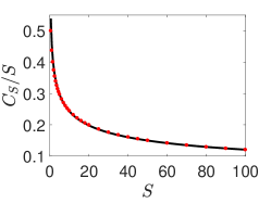
Figure 1: Values of $\tilde{C}_{S}$ for a system of fixed spin $S$. Results are taken from He et al cj-2 .

III.1 Depth of two-mode entanglement

The curves of Figure 1 can be used in a similar way to the Sørensen-Mølmer curves sm-2 to determine a lower bound on the number of boson particles that genuinely comprise a pure two-mode entangled state. This we refer to as the “two-mode entanglement depth”. We note that the number of particles in the entangled state is not simply given by the mean $\langle\hat{N}\rangle$, because in general an experimental system will be a mixture of pure states. It is therefore possible that mixed entangled states with large $\langle\hat{N}\rangle$ arise from highly populated separable states. Such states need only have a small number of particles in the states that are entangled.

As summarised in Section II, the observation $E_{HZ}<1$ implies entanglement between the two modes (and hence the two groups of atoms), which we will refer to as $a$ and $b$ in keeping with the notation for the associated boson operator symbols. Our first result is as follows:

Result (1): If $E_{HZ}$ is measured experimentally, one can determine the maximum value $s_{0}$ such that the following holds:

$$\frac{E_{HZ}}{r}<\tilde{C}_{s_{0}}$$ (11)

where $r=\frac{|\langle\vec{S}\rangle|}{\langle\hat{N}\rangle/2}$. Here we introduce the Bloch vector $\langle\vec{S}\rangle=(\langle\hat{S}_{x}\rangle,\langle\hat{S}_{y}\rangle,\langle\hat{S}_{z}\rangle)$. Hence $|\langle\vec{S}\rangle|=\sqrt{\langle\hat{S}_{x}\rangle^{2}+\langle\hat{S}_{y}\rangle^{2}+\langle\hat{S}_{z}\rangle^{2}}$. We restrict to regimes where $|\langle\vec{S}\rangle|$ is measured to be non-zero. The conclusion from the measurements is that the two-mode entanglement depth is at least $2s_{0}$.

The statement of Result (1) can be clarified for the different contexts of pure and mixed states. If the system were a pure state, then the conclusion is that the system is in a pure bosonic two-mode entangled state which has a mean particle number $\hat{N}$ of at least $2s_{0}$. If the system is in a probabilistic mixture of pure entangled and non-entangled states, then the conclusion is that the system exists, with a nonzero probability $P_{R}$, in a pure two-mode bosonic entangled state $|\psi_{R}\rangle$ of at least $2s_{0}$ particles.

The criteria we derive in this paper apply to all two-mode systems, including photonic systems, for which a mixed state analysis is important. Bose-Einstein condensates prepared experimentally have a high degree of purity, but are nonetheless subject to interactions with the environment that result in a loss of atoms from the condensate. There are hence fluctuations of the atom number $N$ of the condensate. A complete treatment therefore requires consideration of mixed states. Analyses of Bose-Einstein condensates often assume pure states with a fixed atom number $N$. This would imply $P_{R}\sim 1$.

Proof of Result (1): The system is described by a density matrix $\rho=\sum_{R}P_{R}|\psi_{R}\rangle\langle\psi_{R}|$ where $|\psi_{R}\rangle$ is a pure state and $P_{R}$ are probabilities ($\sum_{R}P_{R}=1$, $P_{R}>0$). Each $|\psi_{R}\rangle$ either satisfies a separable model or not. We can write the density operator in the form $\rho=P_{sep}\rho_{sep}+P_{ent}\rho_{ent}$ where $P_{sep}$, $P_{ent}$ are probabilities such that $P_{sep}+P_{ent}=1$. Here $\rho_{sep}$ is a density operator for states described by the separable model. The entangled part of the density operator that does not satisfy the separable model is written

$$\rho_{ent}=\sum_{R^{\prime}}P_{R^{\prime}}|\psi_{R^{\prime}}\rangle\langle\psi_{R^{\prime}}|$$ (12)

where $\sum_{R^{\prime}}P_{R^{\prime}}=1$ and each $|\psi_{R^{\prime}}\rangle$ is an entangled pure two-mode state with $n_{R^{\prime}}$ particles. The expression for $\rho$ that gives the decomposition into a separable and nonseparable part is not required to be unique, as the following proof holds for any such decomposition. Genuine lower bounds can thus be established.

For a mixture the following is true hofmann2

$$(\Delta\hat{S}_{x})^{2}+(\Delta\hat{S}_{y})^{2} \geq \sum_{R}P_{R}\{(\Delta_{R}\hat{S}_{x})^{2}+(\Delta_{R}\hat{S}_{y})^{2}\}$$

where $(\Delta_{R}\hat{S}_{x})^{2}+(\Delta_{R}\hat{S}_{y})^{2}$ is the sum of the variances for the pure state $|\psi_{R}\rangle$. Each state $|\psi_{R}\rangle$ may be written as a linear combination of spin eigenstates $|Sm\rangle$ of $\hat{S}^{2}$ and $\hat{S}_{z}$ (which form a basis). We note however that where $|\psi_{R}\rangle$ is a superposition of states with different $S$, the averages $\langle\hat{S}^{2}\rangle$ and $\langle\hat{S}_{x/y}\rangle$ are equal to those of the corresponding mixtures (because states with different $S$ will be orthogonal) and hence we do not treat this as a special case: It suffices to take a fixed $s_{R}$ for each $|\psi_{R}\rangle$.

We next denote $s_{0}$ as the maximum value of the set $\{s_{R^{\prime}}\neq 0\}$ over the entangled states. If all $s_{R^{\prime}}=0$, then we take $s_{0}=1/2$. Some states may have a zero spin $s_{R}=0$. However, we need only consider the sum over states with $s_{R}\neq 0$ and use the definition $\tilde{C}_{s}=C_{s}/s$, to write:

$$(\Delta\hat{S}_{x})^{2}+(\Delta\hat{S}_{y})^{2} \geq \sum_{R}P_{R}\{\Delta_{R}(\hat{S}_{x})^{2}+(\Delta_{R}\hat{S}_{y})^{2}\}$$ (14)

$$\geq \sum_{R}P_{R}s_{R}\tilde{C}_{s_{R}}$$

The first step remains valid with the restriction to $R$ such that $s_{R}\neq 0$. In the second step, and in all summations over $R$ written below, we take this restriction as implicit. Now we apply the result $\frac{(\Delta\hat{S}_{x})^{2}+(\Delta\hat{S}_{y})^{2}}{|\langle\vec{S}\rangle|}\geq 1$ that holds for the separable states, based on $|\langle\vec{S}\rangle|\leq\langle\hat{N}\rangle/2$ and that separable states satisfy $E_{HZ}\geq 1$. We find

$$(\Delta\hat{S}_{x})^{2}+(\Delta\hat{S}_{y})^{2} \geq P_{sep}\sum_{R^{\prime\prime}}P_{R^{\prime\prime}}s_{R^{\prime\prime}}$$

$$+P_{ent}\sum_{R^{\prime}}P_{R^{\prime}}s_{R^{\prime}}\tilde{C}_{s_{R^{\prime}}}$$

The $C_{S}/S$ functions are monotonically decreasing with $S\neq 0$. This implies that $\sum_{R^{\prime}}P_{R^{\prime}}s_{R^{\prime}}\tilde{C}_{s_{R^{\prime}}}\geq\tilde{C}_{s_{0}}\sum_{R^{\prime}}P_{R^{\prime}}s_{R^{\prime}}$. Hence

$$(\Delta\hat{S}_{x})^{2}+(\Delta\hat{S}_{y})^{2} \geq P_{sep}\sum_{R^{\prime\prime}}P_{R^{\prime\prime}}s_{R^{\prime\prime}}$$

$$+P_{ent}\tilde{C}_{s_{0}}\sum_{R^{\prime}}P_{R^{\prime}}s_{R^{\prime}}$$

Hence

$$(\Delta\hat{S}_{x})^{2}+(\Delta\hat{S}_{y})^{2} \geq \tilde{C}_{s_{0}}\sum_{R}P_{R}s_{R}$$ (15)

$$\geq \tilde{C}_{s_{0}}|\langle\vec{S}\rangle|$$

In the last step we use $\sum_{R}P_{R}s_{R}\geq\sum_{R}P_{R}|\langle\hat{S}_{\theta,\phi}\rangle_{R}|$ where $\langle\hat{S}_{\theta,\phi}\rangle_{R}$ (for the state denoted $R$) is the mean of an arbitrary spin component denoted by $\hat{S}_{\theta,\phi}$, including the $\theta$ and $\phi$ that define the orientation of the Bloch vector $\vec{S}_{R}=(\langle\hat{S}_{x}\rangle_{R},\langle\hat{S}_{y}\rangle_{R},\langle\hat{S}_{z}\rangle_{R})$. This implies $\sum_{R}P_{R}s_{R}\geq\sum_{R}P_{R}|\vec{S}{}_{R}|\geq|\sum_{R}P_{R}\vec{S}{}_{R}|$ and hence $\sum_{R}P_{R}s_{R}\geq|\langle\vec{S}\rangle|$ where $\langle\vec{S}\rangle=\left(\langle\hat{S}_{x}\rangle,\langle\hat{S}_{y}\rangle,\langle\hat{S}_{z}\rangle\right)=\sum_{R}P_{R}\vec{S}_{R}$ is the Bloch vector defined for the state $\rho$. Using the definition of $r$ given by (11), we obtain

$$E_{HZ}\geq r\tilde{C}_{j_{0}}$$ (16)

Thus, if we measure $E_{HZ}<r\tilde{C}_{s_{0}}$, we deduce that one of the pure entangled states $|\psi_{R^{\prime}}\rangle$ must possess a spin greater than $s_{0}$. The number of particles $n_{R^{\prime}}$ in this state $|\psi_{R^{\prime}}\rangle$ is more than $2s_{0}$. This completes the proof.

III.2 Depth of two-mode EPR steering

We note from Figure 1 that in fact $C_{S}<0.5$ for $S>1/2$. It is thus possible to extend Result (1) to include EPR steerable states. We define the two-mode EPR steering depth as the number of boson particles that comprise a pure two-mode EPR steerable state. Next we give the main result of the paper.

Result 2: If the experiment reveals $E_{HZ}<0.5$ , so that we can identify a value $s_{0}$ such that

$$E_{HZ}<r\tilde{C}_{s_{0}}<0.5$$ (17)

where $r=\frac{|\langle\vec{S}\rangle|}{\langle\hat{N}\rangle/2}$, then we deduce a two-mode EPR steering depth of at least $2s_{0}$. If the system were a pure state, the statement means that there is a minimum of $2s_{0}$ particles in the pure two-mode EPR steerable state. If the system is in a mixture $\rho$, then the statement means that (necessarily) there is a nonzero probability $P_{R}$ for the system being in a pure EPR steerable state $|\psi_{R}\rangle$ with at least $2s_{0}$ particles.

Proof of Result (2): We extend the previous proof. In any decomposition of the density operator $\rho=\sum_{R}P_{R}|\psi_{R}\rangle\langle\psi_{R}|$, each $|\psi_{R}\rangle$ either satisfies LHS models (3) and (4) (and is therefore non-steerable), or not. We can write the density operator in the form $\rho=P_{lhs}\rho_{lhs}+P_{st}\rho_{st}$ where $P_{lhs}$, $P_{st}$ are probabilities such that $P_{lhs}+P_{st}=1$. Here $\rho_{lhs}$ is a density operator for states described by the LHS models, which includes all separable states. The steerable part of the density operator that does not satisfy both LHS models (3) and (4) is written

$$\rho_{st}=\sum_{R^{\prime}}P_{R^{\prime}}|\psi_{R^{\prime}}\rangle\langle\psi_{R^{\prime}}|$$ (18)

where $\sum_{R^{\prime}}P_{R^{\prime}}=1$. Here each $|\psi_{R^{\prime}}\rangle$ is an EPR steerable pure two-mode state. Following the proof of Section III.A, we denote $s_{0}$ as the maximum value of the set $\{s_{R}\neq 0\}$ over the steerable states. If all $s_{R^{\prime}}=0$, we take $s_{0}=1/2$. Some states may have a zero spin $s_{R}=0$. However, we consider the sum over states with $s_{R}\neq 0$ and use the definition $\tilde{C}_{s}=C_{s}/s$, to write, following the lines (14), $(\Delta\hat{S}_{x})^{2}+(\Delta\hat{S}_{y})^{2}\geq\sum_{R}P_{R}\{(\Delta_{R}\hat{S}_{x})^{2}+(\Delta_{R}\hat{S}_{y})^{2}\}$. Hence

$$(\Delta\hat{S}_{x})^{2}+(\Delta\hat{S}_{y})^{2}\geq\sum_{R}P_{R}s_{R}\tilde{C}_{s_{R}}$$ (19)

For non-steerable states (which imply that both LHS models (3) and (4) hold), we know from Section II that $E_{HZ}\geq 0.5$. Thus, $\frac{\left(\Delta\hat{S}_{x}\right)^{2}+\left(\Delta\hat{S}_{y}\right)^{2}}{|\langle\vec{S}\rangle|}\geq 0.5$ must hold for the separable and nonsteerable states. We find

$$(\Delta\hat{S}_{x})^{2}+(\Delta\hat{S}_{y})^{2} \geq 0.5P_{lhs}\sum_{R^{\prime}}P_{R^{\prime\prime}}s_{R^{\prime\prime}}$$

$$+P_{st}\sum_{R^{\prime}}P_{R^{\prime}}s_{R^{\prime}}\tilde{C}_{s_{R^{\prime}}}$$

Since $\tilde{C}_{s_{R^{\prime}}}\geq\tilde{C}_{s_{0}}$, this becomes

$$(\Delta\hat{S}_{x})^{2}+(\Delta\hat{S}_{y})^{2} \geq 0.5P_{lhs}\sum_{R^{\prime\prime}}P_{R^{\prime\prime}}s_{R^{\prime\prime}}$$

$$+P_{st}\tilde{C}_{j_{0}}\sum_{R^{\prime}}P_{R^{\prime}}s_{R^{\prime}}$$

Since $\tilde{C}_{s_{0}}\leq 0.5$

$$(\Delta\hat{S}_{x})^{2}+(\Delta\hat{S}_{y})^{2} \geq \tilde{C}_{s_{0}}\sum_{R}P_{R}s_{R}$$ (20)

$$\geq \tilde{C}_{s_{0}}|\langle\vec{S}\rangle|$$

This implies $E_{HZ}\geq r\tilde{C}_{s_{0}}$. Thus, if we measure $E_{HZ}<r\tilde{C}_{s_{0}}$, we deduce an EPR steerable state with spin greater than $s_{0}$, and thus an EPR steerable state $|\psi_{R^{\prime}}\rangle$ with a total number $n_{R^{\prime}}$ of bosons of more than $2s_{0}$. The conclusion is that there is a minimum of $n_{st}=2s_{0}$ bosons involved in the two-mode EPR steerable state. This completes the proof.

III.3 Depth of two-mode EPR steering based on PQS

It is possible to obtain more sensitive criteria for the depth of two-mode steering by considering the lower bounds, derived recently by Vitagliano et al. toth-planar-ent , of $(\Delta\hat{S}_{x})^{2}+(\Delta\hat{S}_{y})^{2}$, for a given $S$ and $\langle S_{||}\rangle=\sqrt{\langle\hat{S}_{x}\rangle^{2}+\langle\hat{S}_{y}\rangle^{2}}$. These authors applied the bounds to deduce large numbers of atoms entangled in an atomic thermal ensemble. In particular, Vitagliano et al. derive convex functions $F_{S}^{(1/2)}$ such that for a fixed $S$

$$\frac{(\Delta\hat{S}_{x})^{2}+(\Delta\hat{S}_{y})^{2}}{\langle\hat{N}\rangle/2}\geq F_{S}^{(1/2)}\Bigl{(}\frac{\langle S_{||}\rangle}{\langle\hat{N}\rangle/2}\Bigr{)}$$ (21)

Here we use the superscript $(1/2)$ to indicate we restrict to spin $1/2$ particles i.e. each particle has two levels (modes) available to it. We prove the following.

Result 3: If the measurement of $E_{HZ}$ and $r_{||}=\frac{|\langle S_{||}\rangle|}{\langle N\rangle/2}$ yield values such that $E_{HZ}<F_{s_{0}}(\frac{|\langle S_{||}\rangle|}{\langle\hat{N}\rangle/2})$ where $F_{S}(x)\leq 0.5$ for all $0\leq x\leq 1$, and if the functions $F_{S}(x)$ are monotonically decreasing with $S$ for every fixed $0\leq x\leq 1$, then the EPR steering depth is (at least) $2s_{0}$. The proof is a straightforward extension of the proofs given in III.B and is given in the Appendix A.

One suitable lower bound are the functions considered by Vitagliano et al of $F_{S}^{(1/2)}(x)=x\zeta_{S}^{2}$, where $\zeta_{S}^{2}$ is the minimum planar spin squeezing value $\xi_{||}^{2}=\frac{\left(\Delta S_{y}\right)^{2}+\left(\Delta S_{z}\right)^{2}}{\left|\left\langle S_{||}\right\rangle\right|}$ over all single particle states $|\psi_{k}\rangle$ of spin $S=k/2$ . Substituting into (21) leads to the condition

$$\frac{E_{HZ}}{r_{||}}<\zeta_{s_{0}}^{2}$$ (22)

for a two-mode $s_{0}$-particle EPR steering depth. Examination of the functions $\zeta_{S}^{2}$ evaluated in Ref. toth-planar-ent reveal similarity with the $\tilde{C}_{S}$ functions (and the Result 2 of Section III.B) associated with the fact that the planar squeezed states minimising $C_{S}$ have Bloch vector orientated along $\vec{S}_{x}$ cj-2 ; hesteer-1 . The values are seen to be monotonically decreasing with $S$ and satisfy $\zeta_{S}^{2}\leq 0.5$, implying the conditions necessary for the Result 3 ($r_{||}\leq 1$).

IV two-mode BEC interferometer

IV.1 Interaction

To illustrate the usefulness of the criteria, we consider a simple model for a two-mode interferometer. For convenience, we symbolise the systems $A$ and $B$ by the notation for the associated boson operators: $a$ and $b$. The two modes become entangled when an initial state consisting of a number state $|N\rangle_{a}$ in mode $a$ and a vacuum state $|0\rangle_{b}$ in mode $b$ are coupled by a $50/50$ beam splitter (Figure 2) hesteer-1 ; noonmesopaper . The state generated after the interaction is

$$|\psi\rangle=\sum_{r}c_{r}|N-r\rangle_{a}|r\rangle_{b}$$ (23)

where $c_{r}=\sqrt{N!}/\sqrt{2^{N}r!(N-r)!}$ noonmesopaper . The state $|\psi\rangle$ is entangled. This can be certified experimentally using the HZ entanglement criterion, $E_{HZ}<1$ hesteer-1 . It was shown in reference hesteer-1 that for $|\psi\rangle$, $E_{HZ}\rightarrow 0.5$ as $N\rightarrow\infty$. This result is plotted in Figure 3. Here $\langle\hat{a}^{\dagger}\hat{a}\rangle=\langle\hat{b}^{\dagger}\hat{b}\rangle$ and hence the steering criterion given by (8) is $E_{HZ}<0.5$, which is not achieved for the simple beam splitter interaction.

The transformations illustrated in Figure 2 also apply to a two-mode BEC atom interferometer. For the details of such interferometers, the reader is referred to Refs. yun-li ; yunli-2 ; Egorov-1 ; Philipp2010-1 ; bjdtwo-mode ; bogdanepl . Here, $N$ atoms are prepared as a single component BEC in the hyperfine atomic level denoted $|1\rangle$. A second atomic hyperfine level is denoted $|2\rangle$. The beam splitter interaction symbolised $BS1$ in the Figure is achieved by a Rabi rotation. This involves application of a $\pi/2$ microwave pulse to the atomic ensemble, to prepare the atoms in a two-component BEC which is in a superposition of the two atomic levels. In a two-mode model, the components of the BEC in levels $|1\rangle$ and $|2\rangle$ are associated with stationary mode functions which we identify respectively as modes $a$ and $b$. The atoms are no longer distinguishable particles but are $N$ bosons of a condensate mode. Comparisons with real interferometers show good agreement with experiment in suitable parameter limits yunli-2 . The two-mode model is relevant only at low temperatures below the critical value where the thermal fraction is negligible. After the interaction denoted $BS1$, the state given by $|\psi\rangle$ can be represented on a Bloch sphere as a spin coherent state. Here, the Bloch vector is aligned along the $x$ direction and has a magnitude $N/2$, and the variances in the $yz$ plane are equal ($(\Delta\hat{S}_{y})^{2}=(\Delta\hat{S}_{z})^{2}$).

The variances required for the $E_{HZ}$ criteria can be measured in terms of number differences at the output of the BEC interferometer. The interferometer has a second beam splitter $BS2$ with the two single mode inputs $a$ and $b$ (Figure 2). Introducing a relative phase shift $\phi$, the boson destruction operators of the output modes of the second beam splitter are $\hat{c}=(\hat{a}-\hat{b}\exp^{i\phi})/\sqrt{2}$, $\hat{d}=(\hat{a}+\hat{b}\exp^{i\phi})/\sqrt{2}$. In the BEC interferometer, the second beam splitter is realised as a second microwave pulse Philipp2010-1 ; Egorov-1 . The output number difference operator is given as $\hat{M}=\hat{d}^{\dagger}\hat{d}-\hat{c}^{\dagger}\hat{c}=2\hat{S}_{x}\cos\phi+2\hat{S}_{y}\sin\phi$. Selecting $\phi=0$ or $\phi=\pi/2$ enables measurements of $\hat{S}_{y}$ or $\hat{S}_{x}$. The $\langle\hat{S}_{z}\rangle$ and $(\Delta\hat{S}_{z})^{2}$ can be measured directly without the second beam splitter, or by passing the outputs $c$ and $d$ through a second transformation with $\phi=0$.

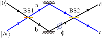
Figure 2: Entangled modes $a$ and $b$ are created when a number state $|N\rangle$ is incident on the beam splitter $BS1$. The entanglement can be detected when the modes $a$ and $b$ interfere across a beam splitter $BS2$ with a phase shift $\varphi$. The two-mode number difference $\hat{M}$ measured at the outputs depends on $\phi$, which enables measurement of the variances $\hat{S}_{x}$, $\hat{S}_{z}$ and $\hat{S}_{x}$. A nonlinear medium may be present after the first beam splitter $BS1$, as modelled by the nonlinear Hamiltonian $H_{NL}$. The description of how the beam splitters are implemented for a BEC interferometer is given in the text.

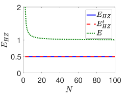
Figure 3: Entanglement between the two modes $a$ and $b$ of the interferometer of Figure 2 in the absence of nonlinearity ($\chi=0$) is detectable by measurement of the Hillary-Zubairy parameter $E_{HZ}$. Also plotted is the value $E_{HZ}^{t}$ for the rotated spin vectors defined in the text, and the ratio $E=|\langle\hat{a}^{\dagger}\hat{b}\rangle|^{2}/\langle\hat{a}^{\dagger}\hat{a}\hat{b}^{\dagger}\hat{b}\rangle$. There is entanglement between the two modes $a$ and $b$ if $E_{HZ}<1$ or $E>1$. $E_{HZ}^{t}<1$ certifies entanglement between the rotated modes defined by Eq. (26).

In order to model the nonlinearity of the atomic medium in a BEC interferometer, we consider that subsequent to the initial Rabi rotation (modelled by $BS1$) the system evolves for a time $t$ according to a nonlinear Hamiltonian

$$H_{NL}=\chi(\hat{a}^{\dagger 2}\hat{a}^{2}+\hat{b}^{\dagger 2}\hat{b}^{2}+2K\hat{a}^{\dagger}\hat{a}\hat{b}^{\dagger}\hat{b}+\hat{a}^{\dagger}\hat{a}+\hat{b}^{\dagger}\hat{b})$$ (24)

Here $K$ is a constant is adjusted to model different atomic interferometers. For $K=-1$ the Hamiltonian reduces to $H_{NL}=\chi(\hat{a}^{\dagger}\hat{a}-\hat{b}^{\dagger}\hat{b})^{2}$ as studied in Refs yun-li . This Hamiltonian is a generalised form of the well-known Josephson Hamiltonian (see ref bjdtwo-mode for a discussion) based on assuming both the mode functions and their occupancy remain fixed. We may also allow $K=0$ to model the interaction $H_{NL}=\chi(\hat{a}^{\dagger}\hat{a})^{2}+(\hat{b}^{\dagger}\hat{b})^{2}$. This interaction is an approximation to the multi-mode BEC interferometer discussed in Ref. bogdanepl . After a time $t$ the state $|\psi\rangle$ evolves to

$$|\psi(t)\rangle = \sum_{r-0}^{\infty}c_{r}e^{-i\Omega(r)t/\hbar}|N-r\rangle_{a}|r\rangle_{b}$$ (25)

where $\Omega(r)=\chi\left[(N-r)^{2}+r^{2}+2Kr(N-r)\right]$ is the term due to nonlinearity. After a time $t$, the second Rabi rotation explained above allows measurement of the spins $\hat{S}_{x}$, $\hat{S}_{y}$ and $\hat{S}_{z}$ and their variances. In the atom interferometer, the number difference is measured by atom imaging techniques.

IV.2 Evolution of $\hat{S}_{x}$, $\hat{S}_{y}$ and $\hat{S}_{z}$

In Figure 4, we plot $E_{HZ}$ and the spin variances for $N=100$, versus $t$ for both $K=-1$ and $K=0$. The solutions show that the Bloch vector is orientated along $\hat{S}_{x}$ ($\langle\hat{S}_{y}\rangle=\langle\hat{S}_{z}\rangle=0$). Initially, $\langle\hat{S}_{x}\rangle\sim N/2$. We plot the evolution of $\langle\hat{S}_{x}\rangle$ noting the drop in value with time. For small times, the solutions show a noise reduction in $\hat{S}_{x}$ with $\Delta\hat{S}_{x}\rightarrow 0$ at $t\rightarrow 0$. Spin squeezing is defined when $(\Delta\hat{S}_{z})^{2}<|\langle\hat{S}_{x}\rangle|/2$ or $(\Delta\hat{S}_{y})^{2}<|\langle\hat{S}_{x}\rangle|/2$. The plots show there is no spin squeezing in $\hat{S}_{z}$ or $\hat{S}_{y}$. The moment $\langle\hat{S}_{z}^{2}\rangle$ is independent of time and also of $\Omega$, for both $K=0$ and $K=-1$. In fact, we find that $(\Delta\hat{S}_{z})^{2}=N/4$. The Figures show that the variance in $\hat{S}_{y}$ can exceed the level of $N/4$.

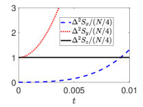
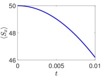
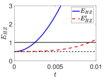
Figure 4: The graphs show the spin variances and mean spin values for the fields created in the nonlinear interferometer of Figure 2 after a time $t$ with nonlinearity present ($\chi\neq 0$). Here time $t$ is in units of $1/\chi$. $N=100$ and $K=-1$. The top left graph gives the variances of $\hat{S}_{x}$, $\hat{S}_{y}$ and $\hat{S}_{z}$. The top right graph shows $\langle\hat{S}_{x}\rangle$. The lower graph gives $E_{HZ}$ and $E_{HZ}^{t}$. Entanglement is signified if $E_{HZ}<1$ or $E_{HZ}^{t}<1$. The plots for $K=0$ are similar but with time in units of $2\chi$.

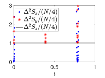
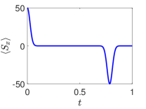
Figure 5: The graphs are as for Figure 4 showing the periodic behaviour that is evident over longer time scales.

Figure 4 also plots the Hillery-Zubairy parameter $E_{HZ}$. The $E_{HZ}$ entanglement value reduces below $1$, due to the smallness of the variance $(\Delta\hat{S}_{x})^{2}$, which is due to the precise number of atoms in the input state $|N\rangle$. This enables a certification of entanglement between modes $a$ and $b$. For longer times, the variances $(\Delta\hat{S}_{x})^{2}$ and $(\Delta\hat{S}_{y})^{2}$ increase sufficiently to destroy the entanglement signature. We also define a rotated $E_{HZ}$ parameter in terms of a different planar spin squeezing orientation, as

$$E_{HZ}^{t}=\frac{(\Delta\hat{S}_{x})^{2}+(\Delta\hat{S}_{z})^{2}}{\hat{N}/2}$$ (26)

Details of the mode transformation assoicated with $E_{HZ}^{t}$ are given in Ref. hesteer-1 . We notice that due to the noise reduction in $\hat{S}_{x}$, both $E_{HZ}<1$ and $E_{HZ}^{t}<1$ for smaller times. The signature for $E_{HZ}^{t}$ lasts longer than that of $E_{HZ}$, due to the stability of the variance $(\Delta S_{z})^{2}$. The solutions for the nonlinear Hamiltonian are periodic as evident from Figure 5, and for longer times there is a return of the entanglement signature $E_{HZ}<1$ and $E_{HZ}^{t}<1$ coinciding with the vector $|\langle\hat{S}_{x}\rangle|\rightarrow N/2$.

IV.3 Spin squeezing of a spin vector in the $yz$ plane

To optimise the detection of EPR-steering using the Hillery-Zubairy entanglement criterion, we seek the optimal spin squeezing for some $\hat{S}_{\theta}$ in the $yz$ plane. In that case, where the variance $\Delta\hat{S}_{x}\rightarrow 0$, the observation of $(\Delta\hat{S}_{\theta})^{2}<N/4$ for $\theta$ in the $yz$ plane would imply an EPR-steering between two appropriately rotated modes. In fact, such spin squeezing has been predicted for the two-mode nonlinear Hamiltonian $H_{NL}$ by Li et al yun-li and has been observed experimentally Philipp2010-1 . With this motivation, we define a spin vector in the $yz$ plane. Thus

$${\color[rgb]{0,0,0}{\color[rgb]{0,0,0}\hat{S}_{\theta}=\hat{S}_{y}\cos\theta+\hat{S}_{z}}\sin\theta}$$ (27)

Spin squeezing in $\hat{S}_{\theta}$ is observed when ueda-1

$$(\Delta\hat{S}_{\theta})^{2}<|\langle\hat{S}_{x}\rangle|/2$$ (28)

We define the spin squeezing ratio

$$\xi_{\theta}^{2}=\frac{(\Delta\hat{S}_{\theta})^{2}}{|\langle\hat{S}_{x}\rangle|/2}$$ (29)

and note that where the Bloch vector is along the $x$ axis and $\langle\hat{S}_{x}\rangle\sim N/2$, this is the definition $\bar{\xi}_{\theta}^{2}=\frac{\left\langle\hat{N}\right\rangle\left(\Delta\hat{S}_{\theta}\right)^{2}}{\left\langle\hat{S}_{x}\right\rangle^{2}}$ used in Refs. ueda-1 . More generally, where $\langle\hat{S}_{x}\rangle<N/2$, we see that $\bar{\xi}_{\theta}^{2}=\frac{\left\langle\hat{N}\right\rangle\xi_{\theta}^{2}}{2|\left\langle\hat{S}_{x}\right\rangle|}>\xi_{\theta}^{2}$ and spin squeezing as defined by $\xi_{\theta}^{2}<1$ does not imply $\bar{\xi}_{\theta}^{2}<1$, though the converse is true. Spin squeezing in $\hat{S}_{\theta}$ is observed when $\xi_{\theta}^{2}<1$. Where $\langle\hat{S}_{x}\rangle=N/2$, there is spin squeezing when $(\Delta\hat{S}_{\theta})^{2}<N/4$. Although not evident in the plots for the $\hat{S}_{z}$ and $\hat{S}_{y}$ of Figures 4 and 5, it is know that spin squeezing is created for optimal $\theta$ by the nonlinear dynamical evolution given by $H_{NL}$. Spin squeezing is predicted by the simple model given by $H_{NL}$, as has been shown in Refs yun-li ; yunli-2 .

We summarise the calculation of Li et al. yun-li ; yunli-2 . We evaluate $(\Delta\hat{S}_{\theta})^{2}=\langle\hat{S}_{\theta}^{2}\rangle-\langle\hat{S}_{\theta}\rangle^{2}$. Here the $\langle\hat{S}_{\theta}\rangle=0$ because $\langle\hat{S}_{y}\rangle=\langle\hat{S}_{z}\rangle=0$. Therefore:

$$\langle\hat{S}_{\theta}^{2}\rangle = \langle\cos\theta\hat{S}_{y}+\sin\theta\hat{S}_{z}\rangle$$ (30)

$$= \frac{1}{2}(\langle\hat{S}_{y}^{2}\rangle+\langle\hat{S}_{z}^{2}\rangle)-C\frac{\cos 2\theta}{2}$$

$$-\frac{i}{4}F\sin 2\theta$$

where we define

$$F = \langle\hat{a}^{\dagger 2}\hat{a}\hat{b}-\hat{a}\hat{b}^{\dagger}-\hat{a}^{\dagger}\hat{a}^{2}\hat{b}^{\dagger}+\hat{b}^{\dagger}\hat{b}(\hat{a}\hat{b}^{\dagger}-\hat{a}^{\dagger}\hat{b})\rangle$$

$$C = \langle\hat{S}_{z}^{2}\rangle-\langle\hat{S}_{y}^{2}\rangle$$ (31)

We wish to find the angle $\theta$ that produces the minimum value of $\langle\hat{S}_{\theta}^{2}\rangle$. We see that

$$\frac{\partial\langle\hat{S}_{\theta}^{2}\rangle}{\partial\theta} = C\sin 2\theta-\frac{iF}{2}\cos 2\theta=0$$ (32)

which implies the stationary condition $\tan 2\theta=\frac{i}{2}\frac{F}{C}$. Therefore the stationary values are at

$$\sin 2\theta = \frac{\pm iF}{\sqrt{4C^{2}+|F|^{2}}}$$

$$\cos 2\theta = \frac{\pm 2C}{\sqrt{4C^{2}+|F|^{2}}}$$ (33)

On substituting into $\langle\hat{S}_{\theta}\rangle$ we find on taking the minimum stationary value

$$\langle\hat{S}_{\theta}^{2}\rangle_{min} = \frac{1}{2}(\langle\hat{S}_{y}^{2}\rangle+\langle\hat{S}_{z}^{2}\rangle)-\frac{4C^{2}+|F|^{2}}{4\sqrt{4C^{2}+|F|^{2}}}$$

Following Li et al., we find significant spin squeezing is possible for an optimal $\theta$ and time $t$. The squeezing versus time is plotted in the Figure 6, as is the optimal angle $\theta$ for the spin squeezing. Figure 7 plots the optimal spin squeezing for a given $N$ in agreement with the plots of Li et al yunli-2 .

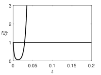
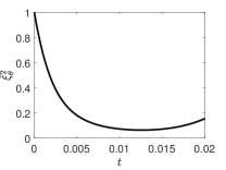
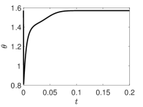
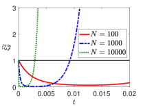
Figure 6: The graphs show the optimal spin squeezing for the fields created in the nonlinear interferometer after evolution for a time $t$, as in the refs. Li et al. yun-li ; yunli-2 . Here time $t$ is in units of $1/\chi$. Top figures show the evolution of spin squeezing as defined by the spin squeezing parameter $\bar{\xi}_{\theta}^{2}$ for $K=-1$ and $N=100$. Spin squeezing is obtained if $\bar{\xi}_{\theta}^{2}<1$. The right graph shows the detail over shorter timescales. The plots of $\xi_{\theta}^{2}$ are indistinguishable from those of $\bar{\xi}_{\theta}^{2}$ over the timescales for squeezing. The lower left graph shows the angle $\theta$ for the optimal squeezing where $N=100$. The lower right graph shows the timescales for higher atom numbers.

The paper Li et al makes a careful comparison between the simplistic two-mode model and more complete models that account for the dynamical changes in the wave function yunli-2 . They evaluate $\chi$ for Rb condensates. Figures 2 and 3 of their paper identify parameter regimes for $N\sim 1000$ atoms where the predictions given by Figure 6 correspond to timescales of order milliseconds and seconds and are in good agreement with the more accurate models.

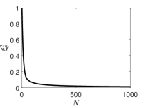
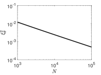
Figure 7: The optimum spin squeezing as defined by the parameter $\bar{\xi}_{\theta}^{2}$ for each value of $N$. Parameters are as for Figure 6. The optimisation is done with respect to time $t$ and angle $\theta$ that defines the squeezing direction.

IV.4 Two-mode EPR steering

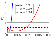
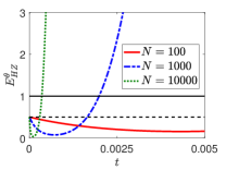
Figure 8: The EPR-steering for optimally rotated modes $c_{\theta}$ and $d_{\theta}$ of the nonlinear interferometer after evolution for a time $t$. The plots show $E_{HZ}^{\theta}$ for the optimal value of $\theta$ at each time $t$ for $N=100,$ $1000$ and $10^{4}$ atoms. Here $K=-1$ and $t$ is in units of $1/\chi$. Entanglement is signified if $E_{HZ}^{\theta}<1$. Steering is signified if $E_{HZ}^{\theta}<0.5$. This implies entanglement and steering between the rotated modes $c_{\theta}$ and $d_{\theta}$ as defined in the text.

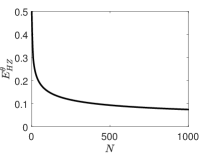
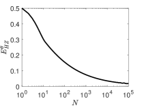
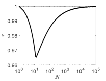
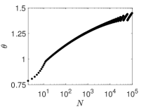
Figure 9: The optimum EPR-steering created in the nonlinear interferometer for a given $N$. Here we optimise with respect to both time $t$ and angle $\theta$. Figures show the optimal value $E_{HZ}^{\theta}$ (top) and the corresponding value of $r=\frac{|\langle\vec{S}\rangle|}{\langle\hat{N}\rangle/2}$ (lower left) for those optimised parameters (right). Here $K=-1$. Entanglement is signified if $E_{HZ}^{\theta}<1$. EPR steering is signified if $E_{HZ}^{\theta}<0.5$. The lower right graph gives the angle $\theta$ that corresponds to the optimal $E_{HZ}^{\theta}$ value for each $N$.

Choosing the direction $\theta$ for optimal squeezing, we can now define the planar spin variance parameter in the plane defined by $x$ and $\theta$ as

$$E_{HZ}^{\theta}=\frac{(\Delta\hat{S}_{x})^{2}+(\Delta\hat{S}_{\theta})^{2}}{\langle\hat{N}\rangle/2}$$ (35)

The $E_{HZ}^{\theta}$ is plotted in Figure 8. The plots show $E_{HZ}^{\theta}<0.5$ indicating EPR steering (see below). However, the EPR steering signature implies EPR steering between two modes $c_{\theta}$ and $d_{\theta}$ that are rotated with respect to $a$ and $b$. We need to define those modes in terms of $a$ and $b$, so that they can spatially separated in a future experiment that may measure an actual EPR steering. In fact, the rotated modes are defined according to boson operators

$$\hat{c}_{\theta} = \cos(\theta/2)\hat{a}+i\sin(\theta/2)\hat{b}$$

$$\hat{d}_{\theta} = i\sin(\theta/2)\hat{a}+\cos(\theta/2)\hat{b}$$

This rotation can be achieved physically by first applying a phase shifting to mode $a$ by $\pi/2$ so that $\hat{a}\rightarrow i\hat{a}$ followed by a rotation of angle $\theta$, to give new modes $\hat{c}^{\prime}=i\cos(\theta/2)\hat{a}-\sin(\theta/2)\hat{b}$ and $\hat{d}^{\prime}=i\sin(\theta/2)\hat{a}+\cos(\theta/2)\hat{b}$. A second phase shift of $-\pi/2$ is applied to the mode $\hat{c}^{\prime}$ so that $\hat{c}^{\prime}\rightarrow-i\hat{c}^{\prime}$ and the final transformation is given by $\hat{c}_{\theta}=\cos(\theta/2)\hat{a}+i\sin(\theta/2)\hat{b}$. Defining spin operators in the new modes: $\hat{S}_{x}^{\theta}=(\hat{c}_{\theta}^{\dagger}\hat{d}_{\theta}+\hat{c}_{\theta}\hat{d}_{\theta}{}^{\dagger})/2$, $\hat{S}_{y}^{\theta}=(\hat{c}_{\theta}^{\dagger}\hat{d}_{\theta}-\hat{c}_{\theta}\hat{d}_{\theta}{}^{\dagger})/(2i)$, $\hat{S}_{z}^{\theta}=(\hat{c}_{\theta}^{\dagger}\hat{c}_{\theta}-\hat{d}_{\theta}{}^{\dagger}\hat{d}_{\theta})/2$, we find

$$\hat{S}_{x}^{\theta} = \hat{S}_{x}$$

$$\hat{S}_{z}^{\theta} = \hat{S}_{z}\cos\theta-\hat{S}_{y}\sin\theta$$

$$\hat{S}_{y}^{\theta} = \hat{S}_{z}\sin\theta+\hat{S}_{y}\cos\theta$$ (36)

We note $\hat{S}_{y}^{\theta}=\hat{S}^{\theta}$ where $\hat{S}^{\theta}$ is defined above by Eq. (27) and thus $(\Delta\hat{S}_{\theta})^{2}=(\Delta\hat{S}_{y}^{\theta})^{2}$. Applying the results summarised in Section II for two-mode systems, we see that entanglement is certified between the modes $c_{\theta}$ and $d_{\theta}$ if one can verify

$$E_{HZ}^{\theta}<1$$ (37)

An EPR-steering ($d$ by $c$) is certified if $E_{HZ}^{\theta}<\frac{\langle\hat{c}^{\dagger}\hat{c}\rangle}{\langle\hat{N}\rangle}$ or ($c$ by $d$) if $E_{HZ}^{\theta}<\frac{\langle\hat{d}^{\dagger}\hat{d}\rangle}{\langle\hat{N}\rangle}$. Since $\langle\hat{c}^{\dagger}\hat{c}\rangle=\langle\hat{N}\rangle/2+\langle\hat{S}_{z}^{\theta}\rangle$ and $\langle\hat{d}^{\dagger}\hat{d}\rangle=\langle\hat{N}\rangle/2-\langle\hat{S}_{z}^{\theta}\rangle$, these criteria for steering can be rewritten as

$$E_{HZ}^{\theta}<\frac{1}{2}\pm\frac{\langle\hat{S}_{z}^{\theta}\rangle}{\langle\hat{N}\rangle}$$ (38)

EPR steering will always be confirmed in at least one direction if $E_{HZ}^{\theta}<0.5$. Hence, since the plots of Figure 8 show $E_{HZ}^{\theta}<0.5$, EPR steering is predicted possible. In fact, we can confirm that in this case, $\langle\hat{c}^{\dagger}\hat{c}\rangle=\langle\hat{d}^{\dagger}\hat{d}\rangle$ and the observation of $E_{HZ}^{\theta}<0.5$ certifies a two-way steering. Figure 9 shows the optimal $E_{HZ}^{\theta}$ values for each $N$.

V Mesoscopic steerable states

We now apply the criterion developed in Sections II and III, to infer the depth of two-mode EPR steering. Figures 10-11 give the calibration showing the effectiveness of the criterion versus $N$, for the steerable states produced by the nonlinear model. The states generated by the Hamiltonian are pure steerable states with a total number of atoms given by $N$. The criterion is used to place a rigorous lower bound based only on the observed experimental variances, without the assumption of a pure state. However a maximally effective criterion would detect a depth of steering of $n_{st}\sim N$. This value is not detected with the criteria, because the states of the interferometer are not the maximal planar spin squeezed states cj-2 . Summarising the Result 2 proved in Section III.B, if we measure $\frac{E_{HZ}}{r}<\tilde{C}_{s_{0}}$ where $\tilde{C}_{s_{0}}=C_{s_{0}}/s_{0}$ and $r=\frac{|\langle\vec{S}\rangle|}{\langle\hat{N}\rangle/2}$, we deduce a depth of EPR steering of (at least) $n_{st}\sim 2s_{0}$.

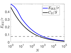
Figure 10: The value of $\frac{E_{HZ}^{\theta}}{r}$ for the interferometer with $N$ atoms is shown by the upper blue line. Here we have evaluated $\frac{E_{HZ}^{\theta}}{r}$ using the angle $\theta$ and time $t$ that minimises the value of $E_{HZ}^{\theta}$ for a given $N$, as displayed in Figure 9. Here $K=-1$. This value may be compared with the fundamental lower value given by the plot of $\tilde{C}_{S}=C_{S}/S$ with $S=N/2$ (lower black line).

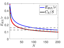
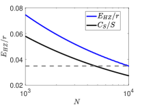
Figure 11: Curves are as in Figure 10. For the left graph, the top horizontal dashed line cuts the $C_{S}/S$ curve just below $C_{S}/S=0.1581$. We see that this value corresponds to $N=2S=42$. Hence if the value $E_{Hz}/r$ is indeed measured, we deduce a steerable state with $n_{st}=42$ atoms. A similar line is drawn for $N=200$ The right graph show the calibration for higher $N$.

In the Figures 10 -12 we plot the predictions for $\frac{E_{HZ}^{\theta}}{r}$ versus $N$ that are shown in Figure 9 for the two-mode BEC atom interferometer. The graphs also show the calibration curves based on the results for $C_{S}/S$ as given in Ref. cj-2 where we have put $N=2S$. These curves extend Figure 1 to larger $S$ and give the fundamental lower bound of the Hillery-Zubairy planar spin squeezing parameter $E_{HZ}/r$. This fundamental lower bound is determined by quantum mechanics. Figure 10 plots the comparison for large values of $N$ based on the analytical expressions given in the paper He et al cj-2 . For high $N$ the lines become indistinguishable on the linear scale for the variances.

$N$	$\frac{E_{HZ}^{\theta}}{r}$	${\color[rgb]{1,0,0}{\color[rgb]{0,0,0}2}}S$	$\tilde{C}_{S}=\frac{C_{S}}{S}$
$50$	$0.1951$	$21$	$0.1952$
$100$	$0.1572$	$42$	$0.1581$
$200$	$0.1261$	$87$	$0.1262$
$500$	$0.0936$	$223$	$0.0938$
$1000$	$0.07457$	$456$	$0.07459$
$10000$	$0.034775$	$4772$	$0.034776$

Table 1: Value of the ratio $\frac{E_{HZ}^{\theta}}{r}$ for different values of $N$. Values of $C_{S}$ for different values of $S$ using the analytical expressions given in the paper He et al cj-2 that corresponds to the minimum value where the condition $\frac{E_{HZ}}{r}<\tilde{C}_{S}$ is satisfied.

Figure 11 gives the close-up of the predictions of $\frac{E_{HZ}^{\theta}}{r}$ for the BEC intereferometer for $N\sim 100-200$ atoms. For a given value of $N$, the predictions may be compared with the plot of $\tilde{C}_{S}=C_{S}/S$ with $N=2S$ given by the lower black line. At $N=100$, we see that $E_{HZ}^{\theta}/r=0.1572$. The horizontal grey dashed line on the graph gives for $N=100$ the minimum value $\tilde{C}_{S}=0.1581$ satisfying the condition (11). We see that this corresponds to $N=2S=42$ on the calibration curve. Hence if the value $E_{HZ}^{\theta}/r$ is indeed measured, one can infer an EPR steerable state with at least $n_{st}=42$ atoms. A similar line is drawn for $N=200$ indicating $n_{st}\geq 87$. The right graph of Figure 11 gives the same analysis but for $N=1000-10,000$ atoms. If the predicted amount of planar spin squeezing $E_{HZ}$ can be observed at $N=10,000$, then it would be possible to deduce mesoscopic steerable states with thousands of atoms. The link between the observed value $\frac{E_{HZ}^{\theta}}{r}$ and the number of atoms that can be inferred is given in the Table I for the range of $N$ that are typical of the spin squeezing experiments.

VI Discussion

There are two main assumptions of the theory given in Section IV of this paper. First, the interferometer is modelled using a simple two-mode Hamiltonian that ignores loss of atoms into other modes, and also ignores the spatial dynamics of the mode functions. More complete treatments show the validity of the approximation, at least for calculations of the spin squeezing, over certain regimes yunli-2 ; bogdanepl ; asinatra . A treatment allowing for changes in both mode occupancy and the mode functions is set out in Ref. bjdtwo-mode . Li et al give a detailed comparison between the two-mode model and more complete models that account for the spatial dynamics. The predictions of the simple model are found to be achievable for Rb condensates of $N\sim 10^{4}$ atoms yunli-2 . The conclusion of the present paper is that one can expect an evolution of the EPR steering correlations over similar timescales as the evolution of spin squeezing. The full calculation however involves the dynamics of the variance associated with the Bloch vector, which was not studied earlier.

At higher temperatures and for larger numbers of atoms, a multi-mode model will be necessary. EPR steering correlations are known to be sensitive to thermal noise, which has not been included in this paper thermal . A multimode treatment that fully accounts for spatial variation of the wavefunctions has been given by Opanchuk et al bogdanepl . The depth of EPR steering criterion used in this paper gives a lower bound of the number of atoms in the two-mode steerable state. Where other modes are present, we point out it is possible to extract the relevant two-mode condensate moments from experimental data, so that the criteria can be applied. This will be discussed in another paper.

The second assumption made in the theory is that there is a fixed number $N$ of atoms incident on the interferometer. While this is typical of many models that have successfully described the evolution of spin squeezing, in practice the fluctuating number input and the inability to fully resolve the atom number on measurement will introduce deviations from the theory. Current experimental strategies do not allow precise control of the number inputs. The effect of number fluctuations on the Hillery-Zubairy entanglement parameter has been studied in the Refs. timpaper-2 ; bogdaneprbec . The variance of $\hat{S}_{x}$ (the Bloch vector) is directly related to the variance of the number input and will increase with increased number fluctuations. Yet, a reduction in the variance for $\hat{S}_{x}$ below the Poissonian level is required for the Hillery-Zubairy EPR steering signature. However, it was also shown in the papers timpaper-2 ; bogdaneprbec that the Hillery-Zubairy criterion can be modified by a normalisation with respect to total number, to give greater sensitivity in the presence of number fluctuations. If the total number of atoms can be accurately counted on detection, then postselection of states with definite $N$ is possible.

VII Conclusion

In summary, we have analysed theory for a two-mode nonlinear interferometer and shown that entanglement and EPR steering correlations between the two modes are predicted. The correlations may be signified by measuring noise reduction in the sum of two spin variances (planar spin squeezing) in accordance with a two-mode Hillery-Zubairy parameter. The required moments are measurable as the population differences at the output of the interferometer, after appropriate phase shifts and re-combinations of the modes. These interactions are realised in atom interferometers as Rabi rotations using microwave pulses.

In principle, it is possible to spatially separate the two modes that show the EPR steering correlations. It is also possible in principle to measure the steering correlations by performing local measurements. This can be seen by expanding the two-mode moments of eqs. (5) and (6) in terms of the local quadrature phase amplitudes. However, the proposal of this paper is to give preliminary evidence of the EPR steering correlations, by recombining the modes at the final beam splitter of the interferometer.

Recent experiments report detection of EPR steering for Bose-Einstein condensates, including for spatial separations. The purpose of our work is to provide a method to extend such analyses, to quantify the number of atoms genuinely comprising the EPR steerable state. The method we give here is based on the lower bounds derived in Ref. cj-2 for an uncertainty relation involving two spins, and would be useful where the steering is identified via planar spin squeezing, or the Hillery-Zubairy parameter.

Appendix A Proof of two-mode depth of steering criterion

Proof: We follow the steps and definitions of the previous proof III.B to arrive at the inequality $(\Delta\hat{S}_{y})^{2}+(\Delta\hat{S}_{z})^{2}\geq\sum_{R}P_{R}\{(\Delta_{R}\hat{S}_{y})^{2}+(\Delta_{R}\hat{S}_{z})^{2}\}$. We find, using (21) and the result for all non-steerable states

$$(\Delta\hat{S}_{y})^{2}+(\Delta\hat{S}_{z})^{2} \geq P_{lhs}0.5\sum_{R^{\prime\prime}}P_{R^{\prime\prime}}s_{R^{\prime\prime}}$$

$$+P_{st}\sum_{R^{\prime}}P_{R^{\prime}}s_{R^{\prime}}F_{s_{R^{\prime}}}\Bigl{(}\frac{\langle S_{||}\rangle_{R^{\prime}}}{s_{R^{\prime}}}\Bigr{)}$$

where here we let $s_{R}=\langle\hat{N}\rangle_{R}/2$. Using that the functions $F_{S}\Bigl{(}\frac{\langle S_{||}\rangle}{S}\Bigr{)}$ are monotonically decreasing with $S,$ for fixed $\frac{\langle S_{||}\rangle_{R^{\prime}}}{s_{R^{\prime}}}$, it follows that

$$(\Delta\hat{S}_{y})^{2}+(\Delta\hat{S}_{z})^{2} \geq P_{lhs}0.5\sum_{R^{\prime\prime}}P_{R^{\prime\prime}}s_{R^{\prime\prime}}$$

$$+P_{st}\sum_{R^{\prime}}P_{R^{\prime}}s_{R^{\prime}}F_{s_{0}}\Bigl{(}\frac{\langle S_{||}\rangle_{R^{\prime}}}{s_{R^{\prime}}}\Bigr{)}$$

(40)

where $s_{0}$ is defined in III.B, as the maximum value of the spins of the set of steerable states. Following the proofs of Refs. sm-2 , we use that the functions $F_{S}$ are convex. Hence they satisfy the inequality $\sum_{k}c_{k}F(x_{k})\geq F(\sum_{k}c_{k}x_{k})$ sm-2 where $c_{k}$ are real numbers. Thus, on introducing $k=\langle\hat{N}\rangle/2$

$$P_{st}\sum_{R^{\prime}}P_{R^{\prime}}s_{R^{\prime}}F_{s_{0}}\Bigl{(}\frac{\langle S_{||}\rangle_{R^{\prime}}}{s_{R^{\prime}}}\Bigr{)} = P_{st}k\sum_{R^{\prime}}\frac{P_{R^{\prime}}s_{R^{\prime}}}{k}F_{s_{0}}\Bigl{(}\frac{\langle S_{||}\rangle_{R^{\prime}}}{s_{R^{\prime}}}\Bigr{)}$$

$$\geq kF_{s_{0}}\Bigl{(}\sum_{R^{\prime}}P_{st}P_{R^{\prime}}\frac{\langle S_{||}\rangle_{R^{\prime}}}{k}\Bigr{)}$$

Thus

$$(\Delta\hat{S}_{y})^{2}+(\Delta\hat{S}_{z})^{2} \geq k\Bigl{(}\sum_{R^{\prime\prime}}P_{lhs}P_{R^{\prime\prime}}\frac{s_{R^{\prime\prime}}}{k}0.5\Bigr{)}$$

$$+kF_{s_{0}}\Bigl{(}\sum_{R^{\prime}}P_{st}P_{R^{\prime}}\frac{\langle S_{||}\rangle_{R^{\prime}}}{k}\Bigr{)}$$

We have taken the case where it is true that $F_{S}\Bigl{(}x\Bigr{)}\leq 0.5$ for all $x$ toth-planar-ent . Thus

$$(\Delta\hat{S}_{y})^{2}+(\Delta\hat{S}_{z})^{2} \geq k\Bigl{(}\sum_{R^{\prime\prime}}P_{lhs}P_{R^{\prime\prime}}\frac{s_{R^{\prime\prime}}}{k}F_{s_{0}}(\frac{\langle S_{||}\rangle_{R^{\prime\prime}}}{s_{R^{\prime\prime}}}\Bigr{)})$$

$$+kF_{s_{0}}\Bigl{(}\sum_{R^{\prime}}P_{st}P_{R^{\prime}}\frac{\langle S_{||}\rangle_{R^{\prime}}}{k}\Bigr{)}$$

Using convexity, we find

$$(\Delta\hat{S}_{y})^{2}+(\Delta\hat{S}_{z})^{2} \geq kF_{s_{0}}(\sum_{R^{\prime\prime}}P_{lhs}P_{R^{\prime\prime}}\frac{\langle S_{||}\rangle_{R^{\prime\prime}}}{k}\Bigr{)}$$ (44)

$$+kF_{s_{0}}\Bigl{(}\sum_{R^{\prime}}P_{st}P_{R^{\prime}}\frac{\langle S_{||}\rangle_{R^{\prime}}}{k}\Bigr{)}$$

$$\geq kF_{s_{0}}\Bigl{(}\sum_{R}P_{st}P_{R}\frac{\langle S_{||}\rangle_{R}}{k}\Bigr{)}$$

$$= \frac{\langle\hat{N}\rangle}{2}F_{s_{0}}\Bigl{(}\frac{\langle S_{||}\rangle}{\langle\hat{N}\rangle/2}\Bigr{)}$$

The last line can be rewritten

$$E_{HZ}^{yz}\geq F_{s_{0}}\Bigl{(}\frac{\langle S_{||}\rangle}{\langle\hat{N}\rangle/2}\Bigr{)}$$ (45)

Violation of this inequality implies the existence of a steerable state with spin $s>s_{0}$, which implies a state with greater than $2s_{0}$ atoms.

Appendix B Evaluation of moments

Here, we show the expressions for the moments evaluated from the Hamiltonian $H_{NL}$ given in Eq. (24). Using the state $|\psi(t)\rangle$ we evaluate the moments needed in the expressions for the variances, $E_{HZ}$ and spin squeezing of Section IV.

$$\langle\hat{a}^{\dagger}\hat{b}\rangle = \sum_{k=0}\sum_{r=0}c_{k}^{*}c_{r}e^{i\left(\Omega(k)-\Omega(r)\right)t/\hbar}\sqrt{N-r+1}\sqrt{r}\times$$

$$\langle N-k|N-r+1\rangle_{a}\langle k|r-1\rangle_{b}$$

$$= \sum_{k=0}c_{k}^{*}c_{k+1}e^{i[\Omega(k)-\Omega(k+1)]t/\hbar}\sqrt{N-k}\sqrt{k+1}$$

$$\langle\hat{a}^{\dagger}\hat{a}\rangle = \langle\hat{b}^{\dagger}\hat{b}\rangle$$

$$= \sum_{r,k=0}c_{k}^{*}c_{r}e^{i\left(\Omega(k)-\Omega(r)\right)t/\hbar}r\langle N-k|N-r\rangle_{a}\langle k|r\rangle_{b}$$

$$= \sum_{r=0}|c_{r}|^{2}r$$

$$\langle\hat{a}^{\dagger}\hat{a}\hat{b}^{\dagger}\hat{b}\rangle = \sum_{r=0}\sum_{k=0}c_{k}^{*}c_{r}e^{i\left(\Omega(k)-\Omega(r)\right)t/\hbar}(N-r)r\times$$

$$\langle(N-k|N-r\rangle_{a}\langle k|r\rangle_{b}$$

$$= \sum_{r=0}c_{r}^{2}(N-r)r$$

$$\langle\hat{a}^{\dagger 2}\hat{a}\hat{b}\rangle = \sum_{r=0}\sum_{k=0}c_{k}^{*}c_{r}e^{i\left(\Omega(k)-\Omega(r)\right)t/\hbar}\left(N-r\right)\times$$

$$\sqrt{N-r+1}\sqrt{r}\langle N-k|N-r+1\rangle_{a}\langle k|r-1\rangle_{b}$$

$$= \sum_{k=0}^{N-1}c_{k}^{*}c_{k+1}e^{i\left(\Omega(k)-\Omega(k+1)\right)t/\hbar}\left(N-k-1\right)C(k)$$

Here we have defined $C(k)=\sqrt{\left(k+1\right)\left(N-k\right)}$.

$$\langle\hat{a}^{\dagger}\hat{a}^{2}\hat{b}^{\dagger}\rangle = \sum_{r=0}\sum_{k=0}c_{k}^{*}c_{r}e^{i\left(\Omega(k)-\Omega(r)\right)t/\hbar}\left(N-r-1\right)\times$$

$$\sqrt{N-r}\sqrt{r+1}\langle(N-k|N-r-1\rangle_{a}\langle k|r+1\rangle_{b}$$

$$= \sum_{r=0}^{N-1}c_{r+1}^{*}c_{r}e^{i\left(\Omega(r+1)-\Omega(r)\right)t/\hbar}\left(N-r-1\right)C(r)$$

Here we have defined $C(r)=\sqrt{N-r}\sqrt{r+1}$.

$$\langle\hat{b}^{\dagger}\hat{b}\hat{a}\hat{b}^{\dagger}\rangle = \sum_{r=0}\sum_{k=0}c_{k}^{*}c_{r}e^{i\left(\Omega(k)-\Omega(r)\right)t/\hbar}\left(r+1\right)\times$$

$$\sqrt{N-r}\sqrt{r+1}\langle(N-k|N-r-1\rangle_{a}\langle k|r+1\rangle_{b}$$

$$= \sum_{r=0}^{N-1}c_{r+1}^{*}c_{r}e^{i\left(\Omega(r+1)-\Omega(r)\right)t/\hbar}\left(r+1\right)C(r)$$

Appendix C Analytical expression for the spin squeezing ratio

Here we show the analytical expressions in order to evaluate the spin squeezing ratio given in Eq. (29) or $\bar{\xi}_{\theta}^{2}=\frac{\left\langle N\right\rangle\left(\Delta S_{\theta}\right)^{2}}{\left\langle S_{x}\right\rangle^{2}}$. Here we used the expression given in Appendix B:

$$\langle\hat{S}_{x}\rangle = \frac{1}{2}(\langle\hat{a}^{\dagger}\hat{b}\rangle+\langle\hat{a}\hat{b}^{\dagger}\rangle)$$

$$= \sum_{r=0}^{N-1}C_{n}C_{n+1}C(r)\cos\left[2(1-K)(N-2r-1)t/\hbar\right]$$

$$= \sum_{r=0}^{N-1}\frac{N!}{2^{N}}\frac{e^{i2\chi(K-1)(N-1-2r)t/\hbar}}{r!(N-r-1)!}\times$$

$$\cos\left[2(1-K)(N-2r-1)t/\hbar\right]$$

$$= \frac{Ne^{-2it(K(N-1)-N-1)}}{2^{N}\left(e^{4iKt}+e^{4it}\right)}\left(e^{4i(K-1)t}+1\right)^{N}$$

Here we have used the definition of $\Omega(r)$, $C_{r}$ and $C(r)=\sqrt{N-r}\sqrt{r+1}$, as well as

$$\langle\hat{a}^{\dagger}\hat{b}\rangle = \sum_{r=0}^{N-1}C_{r}^{*}C_{r+1}e^{i\left[\Omega(r)-\Omega(r+1)\right]t/\hbar}\sqrt{(r+1)(N-r)}$$

$$\Omega(r)-\Omega(r+1)=2(1-K)(N-2r-1)$$

Next, $(\Delta\hat{S}_{\theta})^{2}$ for the optimal angle is $(\Delta\hat{S}_{\theta})^{2}=\langle\hat{S}_{min}\rangle.$ From Eq. (LABEL:eq:mins) we get:

$$\langle\hat{S}_{\theta}^{2}\rangle_{min}=\frac{1}{2}(\langle\hat{S}_{y}^{2}\rangle+\langle\hat{S}_{z}^{2}\rangle)-\frac{\sqrt{4C^{2}+|F|^{2}}}{4}$$

Similar to the case of $\langle\hat{S}_{x}\rangle,$ we use the definition of $\Omega(r)$ and $C_{r}$ as well as the evaluation of the moments given in Appendix A. On simplifying terms we find:

$$\langle\hat{S}_{y}^{2}\rangle = -\frac{1}{4}\langle\hat{a}^{\dagger}\hat{a}^{\dagger}\hat{b}\hat{b}-\hat{a}^{\dagger}\hat{a}\hat{b}\hat{b}^{\dagger}-\hat{a}\hat{a}^{\dagger}\hat{b}^{\dagger}\hat{b}+\hat{a}\hat{a}\hat{b}^{\dagger}\hat{b}^{\dagger}\rangle$$

$$= \frac{1}{8}\{N^{2}+N-4\sum_{r=0}^{N-2}\frac{2^{-N}N!}{r!(N-r-2)!}\times$$

$$\exp\left[-it4(K-1)(N-2(r+1))\right]\}$$

$$= \frac{1}{8}\{N^{2}+N-$$

$$\frac{(N-1)Ne^{4it(-K(N-2)+N+2)}\left(1+e^{8i(K-1)t}\right)^{N}}{2^{N-2}\left(e^{8iKt}+e^{8it}\right)^{2}}\}$$

$$\langle\hat{S}_{z}^{2}\rangle = \frac{1}{4}\langle(\hat{a}^{\dagger}\hat{a}-\hat{b}^{\dagger}\hat{b})\rangle=\frac{N}{4}$$

$$F=\langle\hat{a}^{\dagger 2}\hat{a}\hat{b}-\hat{a}\hat{b}^{\dagger}-\hat{a}^{\dagger}\hat{a}^{2}\hat{b}^{\dagger}+\hat{b}^{\dagger}\hat{b}(\hat{a}\hat{b}^{\dagger}-\hat{a}^{\dagger}\hat{b})\rangle$$

$$=\frac{2^{-N}(N-1)N\left(e^{4it}-e^{4iKt}\right)e^{-2i(K+1)(N-1)t}}{\left(e^{4iKt}+e^{4it}\right)^{2}}\times$$

$$\left(e^{4iKNt}\left(1+e^{4i(1-K)t}\right)^{N}+e^{4iNt}\left(1+e^{4i(K-1)t}\right)^{N}\right)$$

$$C = \langle\hat{S}_{z}^{2}\rangle-\langle\hat{S}_{y}^{2}\rangle$$

$$= \frac{1}{8}[-N^{2}+N+$$

$$\frac{(N-1)Ne^{4it(-K(N-2)+N+2)}\left(1+e^{8i(K-1)t}\right)^{N}}{2^{N-2}\left(e^{8iKt}+e^{8it}\right)^{2}}]$$

If we consider the case where $K=-1$ and $\chi=1$, the above terms can be simplified:

$$\langle\hat{S}_{x}\rangle = (N/2)\cos^{N-1}(4t).$$

$$\langle\hat{S}_{y}^{2}\rangle = \frac{1}{8}\left[N^{2}+N-(N-1)N\left(\cos^{N-2}(8t)\right)\right]$$

$$F = iN(N-1)\left(\cos^{N-2}(4t)\right)\sin(4t)$$

$$C = -\frac{1}{8}\left[N^{2}-N-(N-1)N\left(\cos^{N-2}(8t)\right)\right]$$

Appendix D Discussion of mode entanglement

Entanglement is a feature applying to quantum systems which are composites of two or more physically distinguishable sub-systems. Both the overall system and its sub-systems can be prepared in physically distinct quantum states. For two sub-systems $A,B$, typical pure states for these sub-systems can be listed as $\left|A\right\rangle,\left|B\right\rangle$. Pure states of the overall system are separable if they can be written as $\left|A\right\rangle\otimes\left|B\right\rangle$, otherwise they are entangled. Hence in general $(\left|A_{1}\right\rangle\otimes\left|B_{1}\right\rangle+$ $\left|A_{2}\right\rangle\otimes\left|B_{2}\right\rangle)$ is an entangled state. The definition can be generalised to mixed states, where $\widehat{\rho}_{A},\widehat{\rho}_{B}$ are typical sub-system mixed states. Mixed states are separable if they can be written as $\widehat{\rho}_{A}\otimes\widehat{\rho}_{B}$, otherwise they are entangled. Hence in general $\widehat{\rho}_{A_{1}}\otimes\widehat{\rho}_{B_{1}}+\widehat{\rho}_{A_{2}}\otimes\widehat{\rho}_{B_{2}}$ is an entangled state. We have ignored normalisation. Each sub-system will also be associated with Hermitian operators $\widehat{\Omega}_{A},\widehat{\Omega}_{B}$ representing physical observables for the sub-system, and there will also be Hermitian operators $\widehat{\Omega}$ involving operators from both sub-systems (such as $\widehat{\Omega}_{A}\otimes\widehat{1}_{B}+\widehat{1}_{A}\otimes\widehat{\Omega}_{B})$ that will represent physical observables for the combined system.

In order to define entanglement in many particle systems three issues arise - (1) How do we distinguish sub-systems from each other? (2) Are there requirements that the states and observables for the sub-systems and for the combined system must comply with? (3) How are cases where the number of particles is not definite to be treated? In regard to the third question, experimental situations do in fact arise (such as in BECs) where particle numbers are not well-defined. The second question is underpinned by the requirement that the states for the sub-systems must be physically preparable and the observables physically measureable. The first question reflects the idea that in regard to sub-systems we are referring to an entity which has its own set of physically preparable quantum states and observable quantities, and which can exist independently without reference to other sub-systems. It is particularly important to be precise about what sub-systems are being referred to when discussing entanglement. A quantum state which is entangled when referring to one choice of sub-systems may well be separable when another choice is made - an example is given below. With regard to these questions, there are two extreme situations that could be involved. In the first situation the overall system contains particles that are all identical. In the second situation the overall system contains particles that are all different.

To treat systems of different particles the standard approach is to use the first quantization formalism. Each distinct particle is associated with a set of orthogonal one particle states (or modes) that it can occupy. Note that the choice of modes is not unique - original sets of orthogonal one particle states (modes) may be replaced by other orthogonal sets. However, the single particle states for different particles are obviously distinct from each other. Modes can often be categorized as localized modes, where the corresponding single particle wavefunction is confined to a restricted spatial region, or may be categorized as delocalized modes, where the opposite applies. Single particle harmonic oscillator states are an example of localized modes, momentum states are an example of delocalized modes. Basis states for the overall system or for sub-systems can be obtained as products of the single particle states for each of the different particles involved. Subject to certain restrictions discussed below, general states are quantum superpositions of the basis states. These can represent physically preparable states for either the overall system or for a particular sub-system. Symmetrization principles applying for systems of identical particles are irrelevant, and physical quantities for each sub-system would be based on operators specific to the particles involved (such as the momentum being the sum of momentum operators for each particle), and hence being symmetrical under particle interchange does not apply (Issue 2). Sub-systems are distinguished from each other by just specifying which of the different particles they contain (Issue 1), so sub-systems are defined by particles. Each sub-system would therefore contain just one particle of each of the type involved. Cases where the number of particles differ would be regarded as different systems and each would have its own set of states. Compliance with super-selection rules such as forbidding quantum states that involve coherent superpositions of quantum states for different particles (for example a linear combination of a neutron state with a proton state) can be achieved by simply excluding such states as being unphysical (Issue 2). Although the system is defined by the distinct particles it contains, cases where the number of each particle is not definite can be described via density operators involving statistical mixtures of states with each having precise numbers ($0$ or $1$) of particles of each type (Issue 3).

To treat systems of identical particles it is convenient to use the second quantization formalism. The system is regarded as a quantum field, which is associated with a collection of single particle states (or modes). Again, the choice of modes is not unique - original sets of orthogonal one particle states (modes) may be replaced by other orthogonal sets, and modes may be localised or delocalised. The key requirement is that the modes must be distinguishable from one another, and this enables both the overall system and its sub-systems to be specified via the modes that are involved - hence sub-systems can be distinguished from each other (Issue 1). In this approach, particles are associated with the occupancies of the various modes, so that situations with differing numbers of particles will be treated as differing quantum states of the same system, not as different systems. In second quantization, Fock states defined via the occupancies of the various modes are obtained from the vacuum state (containing no particles in any mode) via the operation of mode creation operators, and such states act as basis states for the quantum system or sub-system being considered. These can represent physically preparable states for either the overall system or a sub-system, and allowed general states are quantum superpositions of the basis states. In linking second and first quantization, the basis states are defined to be in one-one correspondence with the symmetrized products of one particle states that act as the basis states in the first quantization approach. Creation and annihilation operators for each mode are defined to link basis states where the occupancy changes by $\pm 1$. The commutation (anti-commutation) properties of the mode creation and annihilation operators for bosons (fermions) reflect the first quantization requirement that allowed physical states for these systems (and sub-systems) must be symmetric (anti-symmetric) under the interchange of identical particles. Furthermore, physical quantities in the first quantization approach that satisfy the requirement of being symmetric under interchange of identical particles are matched in second quantization by operators based on mode annihilation and creation operators that are constructed to have the same effect on the basis states (Issue 2). Compliance with super-selection rules such as forbidding quantum states that involve coherent superpositions of quantum states with differing numbers of identical particles (for example a linear conbination of a one boson state with a two boson state) can be achieved by simply excluding such states on physical grounds (Issue 2). As the system is defined by the distinct modes it contains, the case where the number of each particle is not definite can be described via density operators involving statistical mixtures of states with each having precise numbers (not restricted to $0$ or $1$, apart from the case of a single mode system for fermions) of particles (Issue 3).

Clearly, for identical particles an approach in which sub-systems are specified by which modes are involved and which is based on using the second quantization formalism is quite suitable for discussing entanglement in such systems, since all three issues are resolved. For distinguishable particles we can treat entanglement using an approach in which sub-systems are specified by which particles are involved and which is based on using the first quantization formalism. For this case the introduction of the second quantization approach would be superfluous. However, because each of the different particles is associated with its own set of single particle states, it follows that defining sub-systems via which particles they contain is actually equivalent to defining them by which modes they contain - so in the distinguishable particles case the particle approach is also equivalent to the mode approach. However, the converse question is – Could the particle approach for defining sub-systems be applied in the identical particles case based on the first quantization formalism? The first problem is that there is no physical method that enables us to distinguish one identical particle from another. In the first quantization formalism we do label each identical particle with a number, but when we then construct basis states with various numbers of particles in the different one particle states, a symmetrization operation is applied that treats them all the same. Similarly, all the physical quantities are based on expressions in which each labelled identical particle is included in the same way. Hence, if sub-systems are defined by which labelled identical particles they contain, then there is an immediate conflict with the requirement of being physically distinguishable from another sub-system which has the same number of differently labelled identical particles. There are of course no numerical labels physically attached to each identical particles - this is just a mathematical fiction. As a result of not being based on distinguishable sub-systems, the labelled identical particle based specification of sub-systems leads to states described in first quantization being regarded as being entangled, whilst exactly the same state described in second quantization (with sub-systems specified by modes) would be regarded as separable. A simple illustration of this contradiction occurs for a system of two bosons, in which one boson occupies a single particle state $\left|\phi_{A}\right\rangle$ and the other occupies a different single particle state $\left|\phi_{B}\right\rangle$. With mode creation operators $\widehat{c}_{A}^{{\dagger}}$ and $\widehat{c}_{B}^{{\dagger}}$, in second quantization the quantum state is given by $\left|\Psi\right\rangle=\widehat{c}_{A}^{{\dagger}}$ $\left|0\right\rangle_{A}\otimes\widehat{c}_{B}^{{\dagger}}$ $\left|0\right\rangle_{B}=\left|1\right\rangle_{A}\otimes\left|1\right\rangle_{B}$, which is a separable state for the combined system consisting of sub-systems specified as modes $\phi_{A}$ and $\phi_{B}$. In first quantization the same state is $\left|\Psi\right\rangle=\left(\left|\phi_{A}(1)\right\rangle\otimes\left|\phi_{B}(2)\right\rangle+\left|\phi_{B}(1)\right\rangle\otimes\left|\phi_{A}(2)\right\rangle\right)/\sqrt{2}$, which would be regarded as an entangled state for the combined system consisting of sub-systems specified by labelled identical particles $1$ and $2$. As the labelled identical particle based specification of sub-systems is in conflict with requirement for sub-systems to be physically distinguishable, we believe that the mode based specification of sub-systems is the correct one to apply in the case of systems consisting of identical particles, and hence it is the approach used in the present paper.

Some confusion can occur when discussing the effect of mode couplers such as beam splitters on a quantum state. In general, the new state may have a different entanglement status for the same pair of sub-system to that of the original state. For the state $\left|\Psi\right\rangle$ above, it is well-known that the effect of a suitable beam splitter could be described by a unitary operator $\widehat{U}$ such that $\widehat{U}\widehat{c}_{A}^{{\dagger}}\widehat{U}^{-1}=(\widehat{c}_{A}^{{\dagger}}+\widehat{c}_{B}^{{\dagger}})/\sqrt{2}$, $\widehat{U}\widehat{c}_{B}^{{\dagger}}\widehat{U}^{-1}=(-\widehat{c}_{A}^{{\dagger}}+\widehat{c}_{B}^{{\dagger}})/\sqrt{2}$. In this case $\widehat{U}$ $\left|\Psi\right\rangle=\left(-\left|2\right\rangle_{A}\otimes\left|0\right\rangle_{B}+\left|0\right\rangle_{A}\otimes\left|2\right\rangle_{B}\right)/\sqrt{2}$, which is now an entangled state for sub-systems specified as modes $\phi_{A}$ and $\phi_{B}$. Thus in general, mode coupling creates entanglement. For a different separable state given by $\left|\Phi\right\rangle=(1/\sqrt{N!})(\widehat{c}_{A}^{{\dagger}})^{N}$ $\left|0\right\rangle_{A}\otimes\left|0\right\rangle_{B}=\left|N\right\rangle_{A}\otimes\left|0\right\rangle_{B}$ the new state for the same beam splitter would be $\widehat{U}\left|\Phi\right\rangle=(1/\sqrt{N!})((\widehat{c}_{A}^{{\dagger}}+\widehat{c}_{B}^{{\dagger}})/\sqrt{2})^{N}(\left|0\right\rangle_{A}\otimes\left|0\right\rangle_{B})$, and again the new state is an entangled state for sub-systems specified as modes $\phi_{A}$ and $\phi_{B}$. However, if we introduce two new orthogonal modes defined by the one particle states $\left|\phi_{C}\right\rangle=(\left|\phi_{A}\right\rangle+\left|\phi_{B}\right\rangle)/\sqrt{2}$ and $\left|\phi_{D}\right\rangle=(-\left|\phi_{A}\right\rangle+\left|\phi_{B}\right\rangle)/\sqrt{2}$, then we see that the new state is also a separable state for sub-systems specified as modes $\phi_{C}$ and $\phi_{D}$, having $N$ bosons in sub-system $\phi_{C}$ and none in sub-system $\phi_{D}$. This is a clear example of a quantum state that is entangled for one choice of sub-systems yet is separable for another choice.

There is however, one situation for a system of identical particles where the particle approach for defining sub-systems is appropriate. This is where the sub-systems each consist of one or more localised modes and the only states considered are where each sub-system just contains one particle. Here each particle may be considered as distinguishable from another one because it is just associated with distinguishable localised modes. This situation applies for certain experiments in quantum information theory, such as where two state identical qubits each involving a single atom are localised by trapping in different places. Reseachers in such quantum information situations generally think of entanglement in terms of separated qubit sub-systems. However, researchers in cold quantum gases are involved with identical particles occupying delocalised modes, so here entanglements is best defined in terms of modal sub-systems.

References

- (1) B. Hensen et al., Nature 526, 682 (2015). M. Giustina et al., 115, 250401 Phys. Rev. Lett. (2015). L. K. Shalm et al., Phys. Rev. Lett. 115, 250402 (2015).
- (2) E. Schrödinger, Naturwiss. 23, 807 (1935).
- (3) B. Julsgaard, A. Kozhekin and E. S. Polzik, Nature 413, 400 (2011). K. C. Lee et al., Science 334 1253 (2011).
- (4) N. J. Engelsen, R. Krishnakumar, O. Hosten and M. A. Kasevich. Phys. Rev. Lett. 118, 140401 (2017).
- (5) J. Estève, C. Gross, A. Weller, S. Giovanazzi, and M. K. Oberthaler, Nature 455, 1216 (2008).
- (6) G. -B. Jo et al., Phys. Rev. Lett, 98 030407 (2007).
- (7) C. Gross, J. Phys. B 45, 1032001 (2012).
- (8) C. Gross, T. Zibold, E. Nicklas, J. Esteve and M. K. Oberthaler, Nature (London) 464, 1165 (2010).
- (9) M. F. Riedel, P. Böhi, Y. Li, T. W. Hänsch, A. Sinatra, and P. Treutlein, Nature (London) 464, 1170 (2010).K. Maussang et al., Phys. Rev. Lett. 105, 080403 (2010).
- (10) C. Gross, H. Strobel, E. Nicklas, T. Zibold, N. Bar-Gill, G. Kurizki and M. K. Oberthaler, Nature 480, 219 (2011).
- (11) J. Peise et al., Nat. Commun. 6, 8984 (2015).
- (12) R. Schmied, J.-D. Bancal, B. Allard, M. Fadel, V. Scarani, P. Treutlein and N. Sangouard, Science 352, 441 (2016).
- (13) B. Lücke et al., Science 334, 773 (2011).
- (14) R. Bücker et al., Nature Physics 7, 608 (2011).
- (15) R. J. Sewell, M. Koschorreck, M. Napolitano, B. Dubost, N. Behbood and M. W. Mitchell, Phys. Rev. Lett. 109, 253605 (2012).
- (16) R. McConnell, H. Zhang, J. Hu, S. Cuk and V. Vuletic, Nature 519, 439 (2015).
- (17) R. I. Khakimov, B. M. Henson, D. K. Shin, S. S. Hodgman, R. G. Dall, K. G. H. Baldwin and A. G. Truscott, Nature 540, 100 (2016).
- (18) P. Kunkel, M. Prüfer, H. Strobel, D. Linnemann, A. Frölian, T. Gasenzer, M. Gärttner and M. K. Oberthaler, Science 360, 413 (2018).
- (19) K. Lange, J. Peise, B. Lücke, I. Kruse, G. Vitagliano, I. Apellaniz, M. Kleinmann, G. Tóth and C. Klempt, Science 360, 416 (2018).
- (20) M. Fadel, T. Zibold, B. Décamps and P. Treutlein, Science 360, 409 (2018).
- (21) A. S. Sørensen and K. Mølmer, Phys. Rev. Lett. 86 4431 (2001).
- (22) G. Vitagliano, G. Colangelo, F. Martin Ciurana, M. W. Mitchell, R. J. Sewell and G. Tóth, Phys. Rev. A 97, 020301 (2018). G. Vitagliano, I. Apellaniz, M. Kleinmann, B. Lücke, C. Klempt and G. Tóth, New J. Phys. 19, 013027 (2017).
- (23) A. Sørensen, L. M. Duan, J. I. Cirac and P. Zoller, Nature 409, 63 (2001).
- (24) A. Einstein, B. Podolsky and N. Rosen, Phys. Rev. 47, 777 (1935).
- (25) J. S. Bell, Physics 1, 195 (1964). N. Brunner et al., Rev. Mod. Phys. 86, 419 (2014).
- (26) E. Schrödinger Proc. Cambridge Philos. Soc. 31, 555 (1935). E. Schrödinger, Proc. Cambridge Philos. Soc. 32, 446 (1936).
- (27) H. M. Wiseman, S. J. Jones and A. C. Doherty, Phys. Rev. Lett. 98, 140402 (2007). S. J. Jones, H. M. Wiseman and A. Doherty, Phys. Rev. A 76, 052116 (2007). D. J. Saunders, S. Jones, H. M. Wiseman and G. J. Pryde, Nature Physics 6, 845 (2010).
- (28) M. D. Reid, Phys. Rev. A 40, 913 (1989). M. D. Reid et al., Rev. Mod. Phys. 81, 1727 (2009).
- (29) E. G. Cavalcanti, S. J. Jones, H. M. Wiseman and M. D. Reid, Phys. Rev. A. 80, 032112 (2009).
- (30) M. Fuwa, S. Takeda, M. Zwierz, H. M. Wiseman and A. Furusawa, Nat. Commun. 6, 6665 (2015). S. Jones and H. M. Wiseman, Phys. Rev. A 84, 012110 (2011). R. Y. Teh, L. Rosales-Zarate, B. Opanchuk and M. D. Reid, Phys. Rev. A 94, 042119 (2016).
- (31) C. Branciard, E. G. Cavalcanti, S. P. Walborn, V. Scarani and H. M. Wiseman, Phys. Rev. A 85, 010301(R) (2012). Q. Y. He, L. Rosales-Zárate, G. Adesso and M. D. Reid, Phys. Rev. Lett. 115, 180502 (2015).
- (32) J. Tura, R. Augusiak, A. B. Sainz, T. Vértesi, M. Lewenstein and A. Acín, Science 344, 1256 (2014). J. Tura, R. Augusiak, A. B. Sainz, B. Lücke, C. Klempt, M. Lewenstein and A. Acín, Ann. Phys. 362, 370 (2015).
- (33) N. Killoran, M. Cramer and M. B. Plenio, Phys. Rev. Lett. 112, 150501 (2014).
- (34) B. J. Dalton, J. Goold, B. M. Garraway and M. D. Reid, Physica Scripta 92, 023005 (2017); ibid, Physica Scripta 92, 023004 (2017).
- (35) Q. Y. He, P. D. Drummond, M. K. Olsen and M. D. Reid, Phys. Rev. A 86 023626 (2012).
- (36) H. Kurkjian, K. Pawłowski and A. Sinatra, Phys. Rev. A 96, 013621 (2017).
- (37) Q. Y. He, M. D. Reid, T. G. Vaughan, C. Gross, M. Oberthaler and P. D. Drummond, Phys. Rev. Lett. 106, 120405 (2011). B. Opanchuk, Q. Y. He, M. D. Reid and P. D. Drummond, Phys. Rev. A 86, 023625 (2012).
- (38) B. J. Dalton, L. Heaney, J. Goold, B.M. Garraway and Th. Busch, New J. Phys., 16, 013026 (2014).
- (39) M. Hillery and M. S. Zubairy, Phys. Rev. Lett. 96, 050503 (2006).
- (40) B. J. Dalton and M. D. Reid, quant-ph arXiv: 1611.09101.
- (41) Q. Y. He, S.-G. Peng, P. D. Drummond and M. D. Reid, Phys. Rev. A 84 022107 (2011).
- (42) M. Kitagawa and M. Ueda, Phys. Rev. A, 47 5138 (1993). D. J. Wineland, J. J. Bollinger, W. M. Itano and D. J. Heinzen, Phys. Rev. A 50, 67 (1994).
- (43) Y. Li, Y. Castin and A. Sinatra, Phys. Rev. Lett. 100, 210401 (2008).
- (44) Y. Li, P. Treutlein, J. Reichel and A. Sinatra. Eur. Phys. J. B 68, 365 (2009).
- (45) B. Opanchuk, M. Egorov, S. Hoffmann, A. Sidorov and P. Drummond, Europhys. Lett., 97 50003 (2012).
- (46) M. Egorov, R. P. Anderson, V. Ivannikov, B. Opanchuk, P. Drummond, B. V. Hall, and A. I. Sidorov, Phys. Rev. A 84, 021605 (2011). M. Egorov, B. Opanchuk, P. Drummond, B. V. Hall, P. Hannaford and A. I. Sidorov, Phys. Rev. A 87, 053614 (2013).
- (47) T. Kovachy, P. Asenbaum, C. Overstreet, C. A. Donnelly, S. M. Dickerson, A. Sugarbaker, J. M. Hogan and M. A. Kasevich, Nature 528, 530 (2015).
- (48) K. S. Hardman, P. B. Wigley, P. J. Everitt, P. Manju, C. C. N. Kuhn and N. P. Robins, Opt. Lett. 41, 2505 (2016).
- (49) Q. Y. He, T. G. Vaughan, P. D. Drummond and M. D. Reid, New J. Phys. 14, 093012 (2012).
- (50) G. Puentes, G. Colangelo, R. J. Sewell and M. W. Mitchell, New J. Phys. 15, 103031 (2013).
- (51) Giorgio Colangelo, Ferran Martin Ciurana, Lorena C. Bianchet, Robert J. Sewell and Morgan W. Mitchell, Nature 543 525 (2017). G. Colangelo, G. Colangelo, F. Martin Ciurana, G. Puentes, M. W. Mitchell and R. J. Sewell, Phys. Rev. Lett. 118, 233603 (2017).
- (52) N. V. Korolkova, Natalia Korolkova, Gerd Leuchs, Rodney Loudon, Timothy C. Ralph, and Christine Silberhorn, Phys. Rev. A 65, 052306 (2002). W. Bowen, Nicolas Treps, Roman Schnabel and Ping Koy Lam, Phys. Rev. Lett. 89, 253601 (2002).
- (53) R. F. Werner, Phys. Rev. A, 40, 4277 (1989). A. Peres, Phys. Rev. Lett. 77, 1413 (1996).
- (54) V. Händchen, T. Eberle, S. Steinlechner, A. Samblowski, T. Franz, R. F. Werner and R. Schnabel, Nat. Photonics 6, 596 (2012). S. L. W. Midgley, A. J. Ferris, and M. K. Olsen, Phys. Rev. A 81, 022101 (2010). J. Bowles, T. Vértesi, M. T. Quintino and N. Brunner, Phys. Rev. Lett. 112, 200402 (2014). S.-W. Ji, M. S. Kim and H. Nha, J. Phys. A 48, 135301 (2015).
- (55) E. G. Cavalcanti, Q. Y. He, M. D. Reid and H. M. Wiseman, Phys. Rev. A84, 032115 (2011).
- (56) H. F. Hofmann and S. Takeuchi, Phys. Rev. A 68, 032103 (2013).
- (57) M. S. Kim, W. Son, V. Bužek, and P. L. Knight, Phys. Rev. A 65, 032323 (2002). B. Opanchuk, L. Rosales-Zárate, R. Y. Teh and M. D. Reid, Phys. Rev. A 94, 062125 (2016).
- (58) B. J. Dalton and S. Ghanbari, J. Mod Opt. 59, 287 (2012), ibid J. Mod. Opt 60, 602 (2013).
- (59) A. Sinatra and Y. Castin, Eur. Phys. J. D 8, 319 (2000).
- (60) Q. Y. He and M.D. Reid, Phys. Rev.A 88, 052121 (2013). L. Rosales-Zárate et al., JOSA B 32 A82 (2015). R. J. Lewis-Swan and K. V. Kheruntsyan, Phys. Rev. A 87, 063635 (2013).