Flux-driven Josephson traveling-wave parametric amplifier

Abstract

We have developed a concept for a traveling-wave parametric amplifier driven by a magnetic-flux wave. The circuit consists of a serial array of symmetric dc SQUIDs coupled inductively to a separate superconducting $LC$ transmission line carrying the pump wave. The adjusted phase velocity of the pump flux-wave of frequency $\omega_{p}$ ensures amplification of the signal ($\omega_{s}$) and the idler ($\omega_{i}$) waves, with frequencies obeying the relation $\omega_{s}+\omega_{i}=\omega_{p}$. The advantage of the proposed flux-driven linear circuit includes a large gain in a wide frequency range and overcoming of the pump depletion problem. Unlike the conventional traveling-wave amplifiers, the signal and pump in the proposed circuit are applied to different ports, what can greatly simplify the whole measurement setup. The experimental parameters and characteristics of this amplifier have been evaluated and show promise for applications in quantum information single-photon circuits.

I Introduction

Josephson parametric amplifiers (JPAs) are among the most useful tools in the field of quantum technology (see, e.g., Refs. Castellanos-Beltran2008 ; Clerk2010 ; Abdo2011 ; Vijay2011 ; Flurin2012 ; Devoret2013 ; Eichler2014 ; Vool2016 ; Lecocq2017 ; Sivak2019 ). However, the quantum-limited performance of these devices is often combined with a fairly limited bandwidth and small dynamic range. The limitation of the bandwidth is primarily due to an amplifier cavity that enhances the interaction between the signal and the pump, thereby ensuring a large parametric gain. For this reason, JPAs that are based on traveling microwaves (i.e., that have no cavity, and are thus free from the gain-bandwidth trade-off) have been extensively explored in the past several years. Mohebbi2011 ; Yaakobi2013 ; OBrien2014 ; White2015 ; Macklin2015 ; Bell-Samolov2015 ; Zorin2016 ; Zorin2017 ; Miano2018 ; WenyuanZhang2017 Moreover, the lack of a cavity enables a larger dynamic range in these amplifiers. OBrien2014

The traveling-wave JPAs (TWJPAs) have an architecture of a microwave transmission line made of periodically repeated sections, including either single Josephson junctions Mohebbi2011 ; Yaakobi2013 ; OBrien2014 ; White2015 ; Macklin2015 or various types of superconducting quantum-interference devices (SQUIDs). Bell-Samolov2015 ; Zorin2016 ; Zorin2017 ; Miano2018 ; WenyuanZhang2017 Most of these amplifiers operate in the four-wave-mixing mode (i.e., when $\omega_{s}+\omega_{i}=2\omega_{p}$, where $\omega_{s}$, $\omega_{i}$, and $\omega_{p}$ are the signal, idler and pump frequencies, respectively). This mode is possible due to the natural Kerr-like nonlinearity of the Josephson inductance $L_{J}=d\Phi(I)/dI$. This inductance, has a quadratic dependence on the reasonably small alternating current $I(t)$ (see, e.g., Refs. Yaakobi2013 ; White2015 ):

$$L_{J}(t)\approx\left[1+0.5I^{2}(t)/I_{c}^{2}\right]L_{J0},$$ (1)

where the parameter $L_{J0}=\varphi_{0}/I_{c}$ is the linear (small-signal) inductance, $\varphi_{0}=\hbar/2e$ is the reduced flux quantum, and $I_{c}$ is the critical current.

Recently, the concept of a TWJPA with three-wave mixing was proposed Zorin2016 and tested. Zorin2017 ; Miano2018 In this amplifier, the frequencies obey the relation $\omega_{s}+\omega_{i}=\omega_{p}$ and the performance is based on the noncentrosymmetric nonlinearity of type $L_{J}^{-1}(\Phi)=dI(\Phi)/d\Phi\approx(1-\beta_{L}\Phi/\varphi_{0})/L\neq L_{J}^{-1}(-\Phi)$ or, equivalently,

$$L_{J}(t)\approx\left[1+\beta_{L}^{2}I(t)/I_{c}\right]L,$$ (2)

which can be engineered with the help of the flux-biased nonhysteretic rf SQUID having linear geometrical inductance $L$ and dimensionless screening parameter $\beta_{L}\equiv LI_{c}/\varphi_{0}<1$ (or, alternatively, by using an asymmetric SQUID having a Josephson kinetic inductance in one branch Sivak2019 ; Zorin2017 ; Frattini2017 ; Frattini2018 ). Compared with the TWJPA with four-wave mixing exploiting Kerr nonlinearity, this three-wave mixing TWJPA was almost free of self-modulation and cross-modulation effects. So, the corresponding wave numbers $k_{s}$, $k_{i}$ and $k_{p}$ did not depend on the pump power $P_{p}$, which may otherwise cause a significant phase mismatch $\Delta k=k_{p}-k_{s}-k_{i}\neq 0$ Agrawal and require careful dispersion engineering (resonant phase matching). White2015 ; Macklin2015

Both these types of TWJPA were based on Josephson nonlinearity (i.e., the dependence of the Josephson inductance $L_{J}(I)$ on current $I(t)$), enabling time-variation of $L_{J}(t)$ with the pump frequency $\omega_{p}$ or the double pump frequency $2\omega_{p}$ in the three-wave-mixing and four-wave-mixing regimes, respectively. The later is the principle of operation of an optical-fiber traveling-wave parametric amplifier Agrawal (as well as a superconducting kinetic-inductance-based traveling-wave parametric amplifier Eom2012 ), where a large pump ensures modulation of the refraction index of optical medium (or kinetic inductance of the wire in the microwave transmission line) with weak Kerr nonlinearity and hence enabling a growth of a signal. Unfortunately, in Josephson parametric amplifiers, the pump power $P_{p}$ (more specifically, the pump current $I_{p}$) is limited by the critical current of the junctions, $\sqrt{P_{p}}\propto|I_{p}|\lesssim 0.5I_{c}$. In addition, the pump power is progressively depleted due to conversion into the signal power $P_{s}$ and the idler power $P_{i}$. This sets a limitation on the length and therefore on the gain of the TWJPA. Thus, similarly to the case of cavity-based JPAs, Kamal2009 ; Abdo2013 the pump depletion reduces the compression point and limits the dynamic range of the TWJPA. OBrien2014 ; Zorin2016 ; Kylemark2006 Finally, the nonlinearity may cause unwanted leakage of the pump power by converting it into power of higher harmonics. White2015 ; Zorin2016

In this paper, we propose an alternative concept for a realization of a TWJPA in which these problems can be mitigated. Our TWJPA uses the principle of straightforward modulation of the Josephson element (dc SQUID) by means of an external flux drive $\Phi_{\textrm{ext}}(t)$, that is,

$$L_{J}(t)=L_{J0}\left[\Phi_{\textrm{ext}}(t)\right],$$ (3)

applied via a separate pump line. In this case, Josephson nonlinearity is no longer used for mixing the modes, so the parametric circuit can operate in the regime with time-varying linear inductance $L_{J}(t)$ and hence have a larger dynamic range.

This fundamental principle of parametric amplification (see, e.g., Refs. Landau-Lifshitz-1 ; Migulin ) was realized by Yamamoto et al. Yamamoto2008 in a cavity-based JPA by directly modulating the flux threading the dc SQUID at twice the resonator frequency. The SQUID in this inherently linear circuit played the role of a flux-dependent inductor terminating a superconducting-transmission-line $\lambda/4$ resonator. The great advantage of this JPA was that the pump and the signal ($\omega_{s}\approx 0.5\omega_{p}$) were applied to different ports of the circuit, so the separation of the output signal from the pump was straightforward. Lately, these flux-driven cavity-based JPAs were successfully applied, for example, for microwave photon generation, Wilson2010 ; Wilson2011 readout of a flux qubit, Lin2013 ultra-sensitive thermal microwave detectors, Simbierowicz2018 and squeezing of vacuum fluctuations. Zhong2013 The nonlinear effects in flux-driven SQUID-based circuits were studied in Refs. Krantz2013 ; Boutin2017 . Another variant of a flux-modulated JPA with high gain was based on eight serially-connected dc SQUIDs that were embedded in a lumped-element $LC$ circuit and driven in phase by an rf current in the common coupling loop. Zhou2014

However, the traveling-wave case is unique in that it requires the flux-drive phases on the individual cells of the SQUID-based transmission line to be properly adjusted. Only then does the parametric amplification of a traveling signal become possible. Below we show that such flux drive is possible with the help of a separate pump transmission line; because this pump line is inductively (weakly) coupled to the signal line over its full length, the flux drive can be realized in the desired traveling-wave fashion. Importantly, in the case of sufficiently small coupling of two lines, the power transmitted in the isolated pump line is no longer limited by the critical current of the Josephson junctions (SQUIDs) inserted in the signal line, but it is limited only by the tolerance of the cryogenic setup to a generated Joule heat. Therefore, sufficiently high pump power can ensure an almost-depletion-free pump regime of parametric amplification. In this case, each elementary cell in the signal line provides the maximum possible gain.

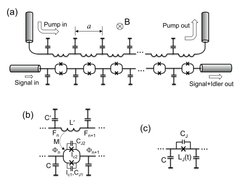
Figure 1: (a) Architecture of a TWJPA driven by means of a flux wave traveling in a separate line. The pump and signal transmission lines consist of similar number $N$ $(\gg 1)$ of identical elementary cells having similar length $a$. A homogeneous static magnetic field B applied perpendicular to the circuit plane sets the constant flux bias $\Phi_{\textrm{dc}}$ and allows adjustment of the SQUID inductances. (Alternatively, the flux bias can be set by a constant feeding current in the pump transmission line.) (b) The pair of inductively coupled elementary cells in the pump and signal lines. (c) Equivalent circuit of the signal-line cell, including ground capacitance $C$ and an effective Josephson junction with self-capacitance $C_{J}$ and time-dependent linear Josephson inductance $L_{J}(t)$.

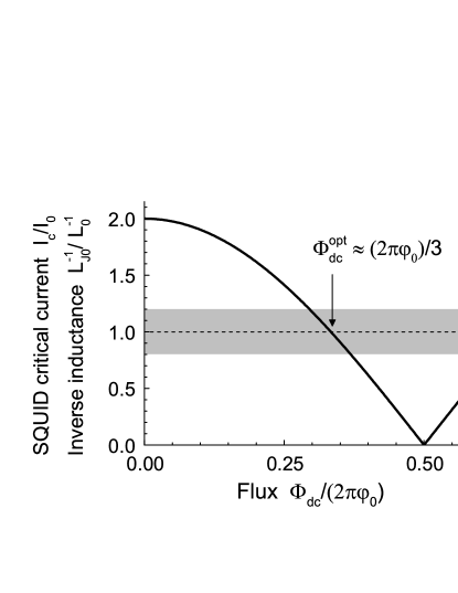
Figure 2: Inverse inductance $L^{-1}_{J0}$ (or critical current $I_{c}$) as a function of the constant flux bias. The shaded band corresponds to the $\pm$20% deviation from the optimal value $1/L_{0}\approx 1/L^{\prime}$ allowing both sufficiently large flux modulation of the inductance and a sufficiently wide range for fine adjustment of the phase velocities in two lines (see Eq. (5)).

II Wave equation and flux drive

The electric diagram of our superconducting microwave circuit with nominally vanishing losses is shown in Fig. 1. The circuit consists of two inductively coupled ladder-type transmission lines: a signal line and a pump line. Similarly to the design of the cavity-based JPA studied in Ref. Castellanos-Beltran2008 , the cells of our signal line include symmetric dc SQUIDs ($I_{c1}=I_{c2}=I_{0}$) with small geometrical inductances of the loops. In this case, the effective critical current $I_{c}=2I_{0}|\cos(\Phi/2\varphi_{0})|$ and the corresponding linear inductance of each SQUID,

$$L^{-1}_{J0}=(2I_{0}/\varphi_{0})|\cos(\Phi/2\varphi_{0})|,$$ (4)

can be efficiently controlled by magnetic flux $\Phi=\Phi_{\textrm{dc}}+\Phi_{\textrm{ac}}$. These SQUIDs are interleaved with identical ground capacitances $C$ (Fig. 1b). The pump transmission line consists of $LC$ sections with inductances $L^{\prime}$ and ground capacitances $C^{\prime}\approx C$; its impedance $Z_{0}=\sqrt{L^{\prime}/C^{\prime}}\approx 50~{}\Omega$. The coupling inductances between SQUIDs and inductors $L^{\prime}$ are equal to $M~{}(\ll L^{\prime})$ and enable ac flux drive in the SQUIDs.

The flux offset $\Phi_{\textrm{dc}}$ is set by means of an external static field B and ensures the SQUID critical current $I_{c}\sim I_{0}$ and hence the SQUID inductance $L_{J0}(\Phi_{\textrm{dc}})\sim L_{0}\equiv\varphi_{0}/I_{0}$. Then, as shown in Fig. 2, the ac component of the flux $\Phi_{\textrm{ac}}$ can result in sufficiently large modulation of the inductance, i.e., $0<L^{-1}_{J0}<2L^{-1}_{0}$. Therefore, efficient three-wave mixing is possible in such a SQUID without use of the nonlinear properties of its inductance. “Fine-tuning” of the flux $\Phi_{\textrm{dc}}$ and therefore the SQUID inductance $L_{J0}\approx L^{\prime}$ allows adjustment of frequencies $\omega_{0}$ and $\omega^{\prime}_{0}$,

$$\omega_{0}=1/\sqrt{L_{J0}C}\approx\omega^{\prime}_{0}=1/\sqrt{L^{\prime}C^{\prime}},$$ (5)

keeping the signal-line impedance $\sqrt{L_{J0}/C}\approx\sqrt{L^{\prime}/C^{\prime}}\approx 50~{}\Omega$. Ignoring for the moment small dispersion, Eq. (5) ensures that the phase velocities of the waves in the signal line,

$$v_{s}=a\omega_{0},$$ (6)

and in the pump line,

$$v_{p}=a\omega^{\prime}_{0},$$ (7)

are equal, where $a$ is the size of the cells in each transmission line. Therefore, spatial phase matching is possible, i.e., $\Delta k=k_{p}-k_{s}-k_{i}\approx 0$.

Generally, the dynamics of the electrical circuit shown in Fig. 1a is described by the set of coupled equations for the values of fluxes $F_{n}$ on the nodes of the pump line and fluxes $\Phi_{n}$ on the nodes of the signal line (see Fig. 1b). These equations are derived in Appendix A. In the case of sufficiently small dimensionless coupling, i.e.,

$$\kappa=M/L^{\prime}\ll 1,$$ (8)

and sufficiently large power $P_{p}$, the pump remains undepleted and presents a traveling flux wave having constant amplitude $A_{p0}\propto\sqrt{P_{p}}$. Then, the equations for these two transmission lines decouple. Eventually, the equation of motion for the signal line in the continuum limit (valid for $\omega\ll\omega_{0},\omega_{J}$) reads

$$\frac{\partial^{2}\phi}{\partial x^{2}}-\omega^{-2}_{0}\frac{\partial^{2}\phi}{\partial t^{2}}+\omega^{-2}_{J}\frac{\partial^{4}\phi}{\partial t^{2}\partial x^{2}}-\gamma\frac{\partial}{\partial x}\left[\left(\frac{\partial\phi}{\partial x}\right)^{3}\right]$$

$$+\frac{\partial}{\partial x}\left[m\sin(k_{p}x-\omega_{p}t)\frac{\partial\phi}{\partial x}\right]=0.~{}~{}$$ (9)

Here, $x$ is the dimensionless coordinate normalized on the cell size $a$; the normalized magnetic flux $\phi(x,t)=\Phi(x,t)/\varphi_{0}$, where the continuous flux variable $\Phi(x,t)$ coincides with flux values $\Phi_{n}$ on the nodes $x=n$. Frequency

$$\omega_{J}=1/\sqrt{L_{J0}C_{J}}$$ (10)

is the plasma frequency of the SQUID, which has total capacitance $C_{J}=C_{J1}+C_{J2}$ (see Fig. 1b) and effective inductance $L_{J0}$. The dimensionless wave numbers of the pump wave in the pump line, $k_{p}$, and of any wave (including signal $\omega_{s}$ and idler $\omega_{i}$) in the signal line, $k$, obey the dispersion relations (see Appendix A)

$$k_{p}\approx\frac{\omega_{p}}{\omega^{\prime}_{0}}\left(1+\frac{\omega_{p}^{2}}{24\omega^{\prime 2}_{0}}\right)\approx\frac{\omega_{p}}{\omega^{\prime}_{0}}\ll 1$$ (11)

and

$$k \approx \frac{\omega}{\omega_{0}}\left(1+\frac{\omega^{2}}{2\omega^{2}_{J}}+\frac{\omega^{2}}{24\omega^{2}_{0}}\right)$$ (12)

$$\approx \frac{\omega}{\omega_{0}}\left(1+\frac{\omega^{2}}{2\omega^{2}_{J}}\right)\ll 1,$$

respectively. The latter relation includes the small term $\omega^{2}/2\omega^{2}_{J}$ which stems from the Josephson plasma resonance in the SQUIDs. Yaakobi2013 The small terms $\omega_{p}^{2}/24\omega^{\prime 2}_{0}$ and $\omega^{2}/24\omega^{2}_{0}$ in Eqs. (11) and (12), respectively, are merely the consequence of the fact that the transmission lines are made of lumped elements. In the practical case of $\omega^{2}_{J}\lesssim\omega^{2}_{0}$, these small terms can be omitted.

The fourth, Kerr-like term (with coefficient $\gamma=1/6$) on the left-hand side of Eq. (9) describes nonlinear effects, Yaakobi2013 which are normally negligibly small (unless the signal amplitude or, more specifically, the Josephson phase difference on the SQUIDs approaches appreciable values, $\varphi(x)=k_{s,i}\Phi(x)/\varphi_{0}\sim 1$; see Section V for more details). For reasonably small input signal, the signal wave can approach such large amplitude only at the transmission-line output. So counting of this term is important only for evaluation of the gain compression.

The fifth term on the left-hand side of the wave equation (9) stems from the time-dependent distributed inductance $L(x,t)$, which is varied in a traveling-wave fashion:

$$L^{-1}(x,t)=[1+m\sin(k_{p}x-\omega_{p}t)]L^{-1}_{J0}.$$ (13)

The dimensionless coefficient $m$,

$$m=\frac{\kappa}{2}A_{p0}k_{p}\tan\frac{\Phi_{\textrm{dc}}}{2\varphi_{0}}\approx\kappa\frac{\sqrt{Z_{0}P_{p}}}{\sqrt{2}\varphi_{0}\omega_{0}}\tan\frac{\Phi_{\textrm{dc}}}{2\varphi_{0}},$$ (14)

determines the depth of the inductance modulation and depends on the strength of coupling $\kappa$ and the pump power $P_{p}$. Here the product $A_{p0}k_{p}$ is equal to $A_{p0}\omega_{p}/\omega_{0}=V_{p}/\varphi_{0}\omega_{0}$, where $V_{p}=\sqrt{2Z_{o}P_{p}}$ is the voltage amplitude in the pump wave.

The time-dependent inductance (13) enables parametric amplification of the signal, Tien1958 ; Cullen1960 ; Boyd2008 given in the ideal case by White2015 ; Zorin2016

$$G = \frac{P^{\textrm{out}}_{s}}{P^{\textrm{in}}_{s}}=\cosh^{2}gN\approx\frac{1}{4}e^{2gN},$$ (15)

$$G_{i} = \frac{P^{\textrm{out}}_{i}}{P^{\textrm{in}}_{s}}=\frac{\omega_{i}}{\omega_{s}}\sinh^{2}gN\approx\frac{\omega_{i}}{4\omega_{s}}e^{2gN},$$ (16)

where both the direct power gain $G~{}(\gg 1)$ and the intermodulation power gain $G_{i}~{}(\gg 1)$ depend exponentially on length $N$ and the gain factor $g\propto m\omega_{p}/\omega_{0}$. Its inverse value,

$$g^{-1}\equiv N_{g},$$ (17)

is therefore the $e$ folding length of the amplitude gain.

III Phase-matching consideration

In the general case, an inherently broadband flux-driven transmission line allows multiwave-mixing processes. Specifically, the basic three-wave mixing process involving conventional idler frequency

$$\omega_{i}=\omega_{p}-\omega_{s},$$ (18)

can be accompanied by two additional mixing processes (frequency up-conversion) involving the idlers  Erickson2017

$$\omega_{1} = \omega_{p}+\omega_{s},$$ (19)

and

$$\omega_{2} = \omega_{p}+\omega_{i}=2\omega_{p}-\omega_{s}.$$ (20)

The latter expression for idler frequency $\omega_{2}$ allows us to interpret the process in Eq. (20) as a four-wave mixing. These three types of mixing [Eqs. (18), (19), and (20)], are schematically shown in Fig. 3a.

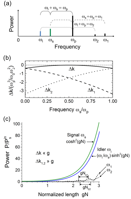
Figure 3: (a) The mixing processes involving the pump frequency ($\omega_{p}$), signal frequency ($\omega_{s}$) and one of three idler frequencies; that is $\omega_{i}$ (solid brackets), $\omega_{1}$ (dashed brackets), and $\omega_{2}$ (dotted brackets). (b) Normalized phase mismatches for the mixing processes (18), (19), and (20) in the case of optimal dc flux offset (ensuring fulfilment of the relation $\omega_{0}-\omega^{\prime}_{0}=\omega^{2}_{p}\omega_{0}/8\omega^{2}_{J}$) as a function of the reduced signal frequency $\omega_{s}/\omega_{p}$. (c) Normalized power of the signal $\omega_{s}$ given by Eq. (15) (solid green line), the idler $\omega_{i}$ given by Eq. (16) (solid blue line) and the idlers $\omega_{1}$ (dashed line) and $\omega_{2}$ (dotted line), as a function of the TWJPA length. Negligibly small phase mismatch $\Delta k$ for the basic process (see Eq. (35)) and large phase mismatches $\Delta k_{1}$ and $\Delta k_{2}$ for the unwanted mixing processes (see Eq. (36)) are assumed. For clarity, the signal frequency is close to $\omega_{p}/2$ (i.e., $\omega_{s}=0.55\omega_{p}$.)

.

If the processes in expressions (19) and (20) are not sufficiently suppressed, they may degrade the amplifier performance. In this general case, the Manley-Rowe relations Manley-Rowe1956 for a pure three-wave-mixing process [Eq. (18)] are modified. Specifically, the original relations for the wave powers, Boyd2008

$$\frac{P_{s}-P^{\textrm{in}}_{s}}{\omega_{s}}=\frac{P_{i}}{\omega_{i}}=-\frac{P_{p}-P^{\textrm{in}}_{p}}{\omega_{p}},$$ (21)

or, equivalently, the relations for the corresponding photon numbers,

$$n_{s}-n_{s}^{\textrm{in}}=n_{i}=n_{p}^{\textrm{in}}-n_{p},$$ (22)

take the form

$$\frac{P_{s}-P^{\textrm{in}}_{s}}{\omega_{s}} = \frac{P_{i}}{\omega_{i}}-\frac{P_{1}}{\omega_{1}}+\frac{P_{2}}{\omega_{2}}$$ (23)

$$= -\frac{P_{p}-P^{\textrm{in}}_{p}}{\omega_{p}}-\frac{2P_{1}}{\omega_{1}}-\frac{P_{2}}{\omega_{2}},$$

or, in terms of the photon numbers,

$$n_{s}-n_{s}^{\textrm{in}}=n_{i}-n_{1}+n_{2}=n_{p}^{\textrm{in}}-n_{p}-2n_{1}-n_{2},$$ (24)

where $P_{1,2}$ and $n_{1,2}$ are the powers and the photon numbers of the modes $\omega_{1,2}$, respectively. Because of large photon energies, $\hbar\omega_{1,2}>\hbar\omega_{p}$, both complementary processes, $\omega_{s,i}+\omega_{p}\rightarrow\omega_{1,2}$ and $\omega_{1,2}\rightarrow\omega_{s,i}+\omega_{p}$, are possible, Yariv1967 so the amplified power of the signal/idler flows repeatedly from mode $\omega_{s,i}$ to mode $\omega_{1,2}$ and vice versa. Boyd2008 ; Yariv1967 This scenario leads to reduction of the direct (intermodulation) gain $G=P^{\textrm{out}}_{s}/P^{\textrm{in}}_{s}$ ($G_{i}=P^{\textrm{out}}_{i}/P^{\textrm{in}}_{s}$). As we show below, suppression of unwanted modes $\omega_{1}$ and $\omega_{2}$ is possible by properly choosing the circuit parameters, i.e., without modification of the circuit architecture.

Using expression (11) for pump-wave number $k_{p}$ and expression (12) for wave numbers $k_{s}$, $k_{i}$, $k_{1}$, and $k_{2}$ of the waves $\omega_{s}$, $\omega_{i}$, $\omega_{1}$, and $\omega_{2}$, respectively, the corresponding phase mismatches for the processes (18), (19), and (20) can be written as

$$\Delta k = k_{p}-k_{i}-k_{s}=\nu-(1/3+\delta^{2})\eta,$$ (25)

$$\Delta k_{1} = k_{p}-k_{1}+k_{s}=\nu-(13/3+4\delta+\delta^{2})\eta,$$ (26)

$$\Delta k_{2} = k_{p}-k_{2}+k_{i}=\nu-(13/3-4\delta+\delta^{2})\eta.$$ (27)

Here the dimensionless frequency detuning is

$$\delta=\frac{2\omega_{s}-\omega_{p}}{\omega_{p}}=\frac{\omega_{p}-2\omega_{i}}{\omega_{p}}.$$ (28)

In Eqs. (25), (26), and (27), we have introduced two small parameters:

$$\eta=3\omega^{3}_{p}/8\omega_{0}\omega^{2}_{J}$$ (29)

and

$$\nu=\omega_{p}/\omega^{\prime}_{0}-\omega_{p}/\omega_{0}\approx\Delta\omega\>\omega_{p}/\omega^{2}_{0},$$ (30)

where $\Delta\omega=\omega_{0}-\omega^{\prime}_{0}\ll\omega_{0}$ is a small mismatch of the cutoff frequencies in two transmission lines (see Eq. (5)). Therefore, properly designing the plasma frequency of the SQUIDs $\omega_{J}$ (see Eq. (10)) and setting a small cutoff-frequency difference, $\Delta\omega>0$, allow effective control of all three phase mismatches (25), (26) and (27). Specifically, fixing the frequency difference as

$$\Delta\omega=\omega^{2}_{p}\omega_{0}/8\omega^{2}_{J},$$ (31)

or, equivalently, taking $\nu=\eta/3$, one can achieve nearly perfect phase matching ($\Delta k\approx 0$) in the basic mixing process (18) for frequencies $\omega_{s}\approx\omega_{i}\approx\omega_{p}/2$ (or small detuning $|\delta|\ll 1$), while keeping appreciable phase mismatches in unwanted processes (19) and (20): that is,

$$\Delta k = -\delta^{2}\eta,$$ (32)

$$\Delta k_{1} = -(4+4\delta+\delta^{2})\eta,$$ (33)

$$\Delta k_{2} = -(4-4\delta+\delta^{2})\eta.$$ (34)

The dependencies of these values on the normalized signal frequency are shown in Fig. 3b.

In the case of sufficiently small $|\Delta k|$, or, equivalently, large coherence length $N_{c}$ in the basic process,

$$N_{c}\equiv\frac{\pi}{|\Delta k|}=\frac{\pi}{\delta^{2}\eta}\gg\frac{1}{g}=N_{g},$$ (35)

and sufficiently short coherence lengths $N_{c1}$ and $N_{c2}$ in two additional mixing processes, i.e.,

$$N_{c1,c2}\equiv\frac{\pi}{|\Delta k_{1,2}|}\approx\frac{\pi}{4\eta}\ll\frac{1}{g}=N_{g},$$ (36)

the unwanted processes (19) and (20) are safely suppressed. So amplification of the signal ($\omega_{s}$) and idler ($\omega_{i}$) frequencies is described by Eqs. (15) and (16), respectively. This favorable case is illustrated in Fig. 3c.

IV Signal gain

To quantify the effect of multiwave mixing (shown schematically in Fig. 3a) we apply the coupled-mode equation method Agrawal . The solution of Eq. (9) is then found in the form of four waves propagating in the forward direction,

$$\phi(x,t)=\frac{A_{s}(x)}{2}e^{i(k_{s}x-\omega_{s}t)}+\frac{A_{i}(x)}{2}e^{i(k_{i}x-\omega_{i}t)}$$

$$+\frac{A_{1}(x)}{2}e^{i(k_{1}x-\omega_{1}t)}+\frac{A_{2}(x)}{2}e^{i(k_{2}x-\omega_{2}t)}+\textrm{c.c.},$$ (37)

where $A_{s}(x)$, $A_{i}(x)$, $A_{1}(x)$, and $A_{2}(x)$ are slowly varying complex amplitudes of the signal and three idlers, obeying the condition Yaakobi2013 ; Zorin2016

$$\left|\frac{\partial^{2}A_{s,i,1,2}}{\partial x^{2}}\right|\ll k_{s,i,1,2}\left|\frac{\partial A_{s,i,1,2}}{\partial x}\right|\ll k_{s,i,1,2}^{2}\left|A_{s,i,1,2}\right|.$$ (38)

After incorporation of Eq. (37) into Eq. (9) with the omitted Kerr term ($\propto\gamma$), the coupled linear equations for $A_{s}$, $A_{i}$, $A_{1}$, and $A_{2}$, take the form

$$\frac{dA_{s}}{dx} = \frac{m}{2}k_{i}A^{*}_{i}e^{i\Delta kx}+\frac{m}{2}k_{1}A_{1}e^{-i\Delta k_{1}x},$$ (39)

$$\frac{dA_{i}}{dx} = \frac{m}{2}k_{s}A^{*}_{s}e^{i\Delta kx}+\frac{m}{2}k_{2}A_{2}e^{-i\Delta k_{2}x},$$ (40)

$$\frac{dA_{1}}{dx} = -\frac{m}{2}k_{s}A_{s}e^{i\Delta k_{1}x},$$ (41)

$$\frac{dA_{2}}{dx} = -\frac{m}{2}k_{i}A_{i}e^{i\Delta k_{2}x}.$$ (42)

The first terms on the left-hand-sides of Eqs. (39) and (40), describe the basic parametric mixing (18). Agrawal

In the case of sufficient suppression of modes $\omega_{1}$ and $\omega_{2}$ (see Eq. (36) or, equivalently, the inequality $\pi g/4\eta\ll 1$) small amplitudes $A_{1}$ and $A_{2}$ can be omitted and the decoupled pair of equations (39) and (40) for solely amplitudes $A_{s,i}$ has a simple analytical solution. Specifically, the solution with initial conditions $A_{s}(0)=A_{s0}$ and $A_{i}(0)=0$ reads White2015 ; Zorin2016

$$A_{s} = A_{s0}\left[\cosh gx-i\frac{\Delta k}{2g}\sinh gx\right]e^{i\Delta kx/2},~{}~{}$$ (43)

$$A_{i} = 2\frac{g_{0}\omega_{s}}{g\omega_{p}}A_{s0}\sinh(gx)e^{i\Delta kx/2}.$$ (44)

Here the exponential gain factor is

$$g=\sqrt{(1-\delta^{2})g_{0}^{2}-(\Delta k/2)^{2}},$$ (45)

and its maximum value,

$$g_{0}=\frac{mk_{p}}{4}\approx\frac{m\omega_{p}}{4\omega_{0}},$$ (46)

is achieved at perfect phase matching, $\Delta k=0$, and zero detuning, $\delta=0$.

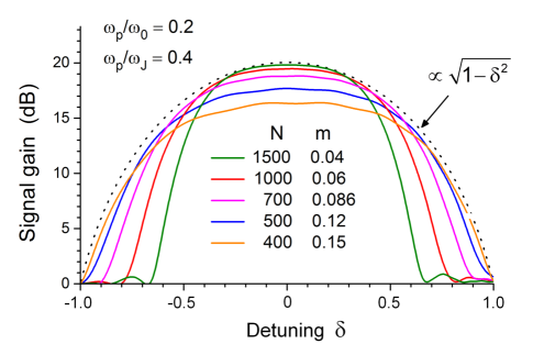
Figure 4: Signal gain as a function of frequency $\omega_{s}$ at fixed pump frequency $\omega_{p}=0.2\omega_{0}$ and Josephson plasma frequency $\omega_{J}=0.5\omega_{0}$ (yielding $\eta=0.012$, see Eq. (29)). Solid curves correspond to several combinations of length $N$ (in decreasing order from top to bottom) and modulation parameter $m$ with fixed product $g_{0}N=m\omega_{p}N/4\omega_{0}=3$ (yielding nominal maximum gain of $G=\cosh^{2}g_{0}N\approx 10^{2}$). The dotted curve shows the ultimate gain versus frequency given by Eq. (48).

The power gain $G$ of the line of length $N$ is then given by formula White2015

$$G=\frac{|A_{s}(N)|^{2}}{|A_{s0}|^{2}}=\cosh^{2}gN-\left(\frac{\Delta k}{2g}\right)^{2}\sinh^{2}gN,$$ (47)

which for zero phase mismatch, $\Delta k=0$, and large gain, $gN\gg 1$, is reduced to Eq. (15) with $g=g_{0}\sqrt{1-\delta^{2}}$, i.e.,

$$G=\cosh^{2}(g_{0}\sqrt{1-\delta^{2}}N)\approx\frac{1}{4}\exp\left(\frac{\omega_{p}\sqrt{1-\delta^{2}}}{2\omega_{0}}mN\right).$$ (48)

The frequency dependence of $\log G$ has a typical semicircle shape, $y=\sqrt{1-\delta^{2}}$, with the maximum at $\delta=0$. Tien1958 ; Cullen1960 For example, the amplifier with this ideal shape of the power gain with maximum value of 20 dB has a 3-dB bandwidth of $\sqrt{1-(17/20)^{2}}\,\omega_{p}\approx 0.5\omega_{p}$, which is centered at $\omega_{s}=0.5\omega_{p}$ (see the dotted line in Fig. 4). Cullen1960 ; Zorin2016 .

In the case of insufficiently short coherence lengths $N_{c1}$ and $N_{c2}$ [i.e. only slightly less than or approximately equal to $N_{g}$; see Eq. (36)], that is, a not sufficiently small value of the dimensionless parameter

$$\xi=\frac{N_{c1,c2}}{N_{g}}=\frac{\pi g_{0}\sqrt{1-\delta^{2}}}{4\eta}\approx\frac{m\omega^{2}_{J}\sqrt{1-\delta^{2}}}{2\omega^{2}_{p}}\lesssim 1,$$ (49)

the power conversion to the modes $\omega_{1}$ [Eq. (19)] and $\omega_{2}$ [Eq. (20)] becomes appreciable. So, redistribution of power between the signal, the idler and the unwanted idler modes $\omega_{1}$ and $\omega_{2}$ may lead to substantial suppression of the signal gain. To quantify this effect, which is most pronounced at large detuning, $|\delta|\geq 0.5$, we numerically solve the set of differential equations (39)-(42).

Figure 4 shows the frequency dependence of $\log G$ obtained by numerical integration of Eqs. (39)-(42) with initial conditions

$$A_{s}(0)=A_{s0},~{}~{}~{}A_{i}(0)=A_{1}(0)=A_{2}(0)=0,$$ (50)

for five TWJPAs having different lengths $N$ (the set of solid curves), but nominally the same maximum gain of 20 dB (adjusted by a proper pump power, $P_{p}\propto 1/N^{2}$, keeping $m\propto 1/N$). We find $\xi$ is approximately equal to 0.13, 0.19, 0.27, 0.38, and 0.47 (in the order of the curves from top to bottom in the central part of the plot) which cover the range from the relatively small value of 0.13 up to the value 0.47 close to unity. For comparison, the dotted curve illustrates the case of $\xi=0$, yielding the maximum possible gain given by Eq. (48).

One can see two features in the behavior of these circuits. Firstly, the gain suppression in the TWJPAs with relatively small values of $\xi$ ($\xi<0.3$ or $m<0.1$) is rather small ($<2$ dB) for detuning $|\delta|\lesssim 0.5$, whereas for $0.5\lesssim|\delta|\leq 1$ the gain suppression is significant. This behavior is due to increase of the phase mismatch $|\Delta k|=\delta^{2}\eta$ and hence violation of inequality (35) occurring at relatively large $|\delta|$. Secondly, the signal gain for rather large values of $\xi$ ($\xi>0.3$ or $m>0.1$) is notably less than the nominal value given by the dotted line, especially for small detuning, $|\delta|\lesssim 0.5$. That suppression of the gain for larger detuning, $|\delta|\gtrsim 0.5$, is not so dramatic as in the case of small $\xi$. So, we can conclude that for our set of characteristic frequencies, a TWJPA length $N$ of about 1000 ensures both sufficiently large bandwidth of about $0.47\omega_{p}$ and sufficiently small unwanted power conversion to the high-frequency idler modes.

V Possible circuit design

The design of the practical circuit obviously depends on specific applications of the TWJPA. Below we focus on the set of parameters typical for the TWJPAs (both with three-wave mixing and four-wave mixing) that were earlier developed for the quantum-information applications including superconducting qubits. OBrien2014 ; White2015 ; Macklin2015 ; Bell-Samolov2015 ; Zorin2016 ; Zorin2017 ; Miano2018 ; WenyuanZhang2017 These parameters include an operation frequency on the order of 10 GHz, relatively large Josephson junctions having critical current on the order of several microamperes (and hence sufficiently low charging energy $E_{c}=e^{2}/2C_{J}\sim 10^{-3}\varphi_{0}I_{0}$, ensuring classical behavior of the Josephson phase $\varphi$), a standard line impedance of 50 $\Omega$, and a nominal gain of 20 dB.

Taking a relatively high target value of the cutoff frequency $\omega_{0}/2\pi=100$ GHz and the standard transmission-line impedance $Z_{0}=50~{}\Omega$, we obtain the following basic circuit parameters,

$$C^{\prime}=C=1/\omega_{0}Z_{0}\approx 32~{}\textrm{fF}$$ (51)

and

$$L^{\prime}=L_{J0}=Z_{0}/\omega_{0}\approx 80~{}\textrm{pH}.$$ (52)

For a typical size of an elementary cell $a\sim 30~{}\mu$m (see possible circuit layout, for example, in Ref. Zorin2017 ) the phase velocity of microwaves in these transmission lines $v_{s}=a\omega_{0}$ is reduced to about 2$\times 10^{7}$ m/s. The wavelength of the pump $\lambda_{p}$ for the designed frequency of $\omega_{p}/2\pi=20$ GHz (i.e., $\omega_{p}/\omega_{0}=0.2$) is equal to the length of $N_{p}=2\pi\omega_{0}/\omega_{p}\approx 31$ elementary cells.

In the optimal working point the constant magnetic flux $\Phi^{\textrm{opt}}_{\textrm{dc}}/2\varphi_{0}\approx\pi/3$ yields about 50 % suppression of the maximum critical current of the SQUIDs, so the Josephson inductance [Eq. (52)] corresponds to the critical current of a single junction, i.e., $I_{0}=\varphi_{0}/L_{J0}\approx 4~{}\mu$A (see Fig. 2). Such Josephson junctions can be fabricated using either multilayer niobium technology (see, e.g., Refs. Dolata2005 ; Tolpygo2017 ) or shadow-evaporation aluminum technology. Niemeyer1974 The Josephson plasma frequency of a bare Josephson junction with critical current density of, say, $j_{c}=3~{}\mu\textrm{A}/\mu\textrm{m}^{2}$ and specific barrier capacitance about $c_{J}=50$ fF/$\mu\textrm{m}^{2}$ is $\sqrt{j_{c}/\varphi_{0}c_{J}}/2\pi\approx 70$ GHz. van-der-Zant1994 Therefore, the plasma frequency of the flux-biased SQUID with a partially suppressed critical current is $\omega_{J}/2\pi\approx 70\sqrt{\cos(\pi/3)}~{}\textrm{GHz}\approx 50$ GHz, i.e., $\omega_{p}/\omega_{J}=0.4$. Taking the total number of elementary cells $N=1000$, one can achieve sufficiently large gain in a reasonably large bandwidth (see Fig. 4). Possible deterioration of performance due to imperfect flux setting and inhomogeneity of the transmission-line parameters (including those due to regular and irregular inhomogeneities of the critical current density on the chip) should be sufficiently small. The corresponding estimations are given in Appendix B.

According to formula (14), the target value of the modulation parameter $m=0.06$ can be achieved by engineering a reasonably small dimensionless coupling $\kappa=M/L^{\prime}$ (e.g., on the order of 0.02) and applying sufficiently large pump power,

$$P_{p}=2\cot^{2}(\pi/3)\frac{(m\varphi_{0}\omega_{0})^{2}}{\kappa^{2}Z_{0}}\approx-53~{}\textrm{dBm}.$$ (53)

This power passing though the superconducting transmission line is not immediately dissipated on the chip, but can cause some heating of cold attenuators installed in the base-temperature stage. However, this level of power is seemingly acceptable for the most of setups with dilution refrigerators.

In conventional TWJPAs operating on the basis of wave mixing with the aid of Josephson nonlinearity, a relatively small pump power (limited by the nonlinear-element characteristics, i.e., the critical current) propagates together with the signal and idler waves in the common transmission line. Because of parametric interaction of these traveling waves the pump power is gradually converted into the signal and the idler. The resulting pump depletion leads to gradual reduction of the signal gain and, finally, to gain saturation. This effect dramatically limits the amplifier dynamic range. OBrien2014 ; Zorin2016 The important feature of the proposed TWJPA driven by relatively large power (53) fed into a separate port of an isolated $LC$ line and only partly converted into the signal and idler is almost constant pump power (i.e., the absence of pump depletion). This remarkable property enables ultimate mixing in all section of the signal line and, hence, a steady gain. Only at sufficiently large signal amplitude achieved in the output sections of the line (i.e., for ac amplitude amounting to about $I_{0}$) is its further growth impeded by the SQUID nonlinearity.

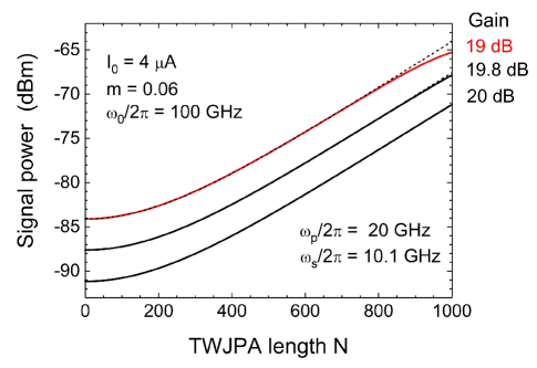
Figure 5: Increasing power of the signal waves of frequency $\omega_{s}=0.505\omega_{p}$ with input powers of $-91$ dBm, $-87.7$ dBm, and $-84$ dBm (solid lines in the order from bottom to top, respectively) as a function of the cell number [found by numerical solution of the coupled-mode nonlinear equations (54) and (55)]. The actual gain for different input powers is given in the right column. The topmost solid curve (red) corresponds to decrease of the nominal 20-dB gain by 1 dB, which occurs at input power $P_{1\textrm{dB}}=-84$ dBm. For comparison, the dashed lines show the signal-power growth ignoring the nonlinear effects ($\gamma=0$); that is, applying the formula $P_{s}=P^{\textrm{in}}_{s}\cosh^{2}g_{0}N$ (see Eq. (48)).

To evaluate this effect in the limit of pure three-wave mixing ($|A_{1,2}|\ll|A_{s,i}|$), we derive from Eq. (9) the pair of coupled nonlinear equations for complex amplitudes $A_{s}$ and $A_{i}$:

$$\frac{dA_{s}}{dx}=\frac{m}{2}k_{i}A^{*}_{i}e^{i\Delta kx}+i\frac{3}{8}\gamma k_{s}A_{s}(k_{s}^{2}|A_{s}|^{2}+2k_{i}^{2}|A_{i}|^{2}),\;$$ (54)

$$\frac{dA_{i}}{dx}=\frac{m}{2}k_{s}A^{*}_{s}e^{i\Delta kx}+i\frac{3}{8}\gamma k_{i}A_{i}(k_{i}^{2}|A_{i}|^{2}+2k_{s}^{2}|A_{s}|^{2}).\;\;$$ (55)

The self-Kerr ($\propto\gamma A_{s,i}|A_{s,i}|^{2}$) and the cross-Kerr ($\propto\gamma A_{s,i}|A_{i,s}|^{2}$) nonlinear terms both cause the effect of phase modulation Agrawal and hence phase mismatch, $\Delta k\neq 0$, White2015 ; Macklin2015 ; Bell-Samolov2015 ; Zorin2016 rising with the growth of the signal and the idler. As result, the total gain of TWJPA is reduced. We solve Eqs. (54) and (55) with initial conditions $A_{s}(0)=A^{\textrm{in}}_{s}=\sqrt{2Z_{0}P^{\textrm{in}}_{s}}/\omega_{s}\varphi_{0}$ and $A_{i}(0)=0$ numerically and present the results in Fig. 5.

The plot shows almost exponential growth of the signal power propagating in the array of SQUIDs with effective critical current $I_{0}=4~{}\mu$A and driven by the flux wave ensuring the modulation-parameter value $m=0.06$. One can see that for sufficiently small input power the amplifier shows a nominal gain of about 20 dB (see the bottom curve, corresponding to $P^{\textrm{in}}_{s}\approx-91$ dBm and $P^{\textrm{out}}_{s}\approx-71$ dBm). For somewhat larger input power values (see, e.g., the middle curve with $P^{\textrm{in}}_{s}\approx-88$ dBm the suppression of the nominal gain is still rather small (i.e., about $-0.2$ dB). In this case, the amplitude of current oscillations in the output sections of the signal transmission line approaches approximately $0.7I_{0}$, whereas the Josephson phase oscillations are about $\pi/4$.

The upper solid curve, calculated for the largest input power of $P_{\textrm{1dB}}\approx-84$ dBm, exhibits 1-dB suppression of the nominal gain of 20 dB and hence corresponds to the amplifier compression point. In this case, the signal current amplitude in the output sections of the line approaches approximately $0.9I_{0}$ leading to an amplitude of the Josephson phase oscillations of about 1.1 rad. At such large amplitude the cubic approximation of the Josephson nonlinearity in the original wave equation (9) is no longer strictly valid, so the above-mentioned value of $-84$ dBm can be considered only as an estimate of the gain compression point. Still, this value is broadly larger than that achievable in nonlinearity-based TWJPAs with almost similar electrical parameters (both with four-wave mixing and three-wave mixing). For example, the gain compression points reported in Refs. OBrien2014 ; Zorin2016 are $-98$ dBm (for $I_{0}=3.29~{}\mu$A) and $-96$ dBm (for $I_{0}=5~{}\mu$A), respectively.

The reason for the notable increase of the amplifier dynamic range is the almost absence of pump depletion. In the above example, the maximum output signal power is sufficiently small (i.e., $P^{\textrm{out}}_{s}+P^{\textrm{out}}_{i}\approx 2P^{\textrm{out}}_{s}\approx-62~{}\textrm{dBm}\ll P_{p}=-53~{}\textrm{dBm}$) and is set by saturation in the last sections of the line, as one can conclude from comparison of the solid and dashed lines in Fig. 5. This property allows us to achieve signal gain in the most-efficient way.

VI Conclusion and prospects

We develop a concept for a flux-driven TWJPA with a large dynamic range. Due to the separate transmission-line, fed through an isolated input port by sufficiently large pump power, the amplifier is practically free of the pump-depletion effect. Moreover, the linear regime of its operation ensures small distorsions of signal, which prevents the generation of shock waves. Landauer1960 Because of good phase matching in a rather broad bandwidth, these properties allow parametric amplifiers to be designed with rather large number of elementary cells $N$ and therefore larger gain (e.g., 40 dB). In combination with ultimately quantum-limited performance over a wide frequency range, such a TWJPA could be an indispensable device for amplifying weak signals from quantum sources, including qubits.

When required, even larger output signals can be achieved by using in each elementary cell not of a single SQUID but of a group of several serially connected SQUIDs (as reported in Ref. Zhou2014 ) designed with Josephson junctions having larger critical currents and therefore weaker (unwanted) Kerr nonlinearity. In this case, the need for a cold HEMT preamplifier with typical noise figure of several kelvins, which is usually unavoidable in high-fidelity microwave measurements, is eliminated. The latter feature may be especially useful in quantum-information processing and, in particular, in quantum-interference and quantum-correlation measurements with single microwave photons. Bozyigit2010 ; Peng2016

The proposed circuit may also operate in the quantum regime enabling efficient production of entangled photon pairs. As recently demonstrated by Lahteenmäki et al., Lahteenmaki2013 a similar array of 250 dc SQUIDs, embedded in a microwave resonator and pumped by homogeneous alternating flux at the double resonant frequency of $2\omega_{\textrm{res}}=2\pi\times 10.8$ GHz, gave rise to the generation of biphotons at frequencies $\omega_{a}$ and $\omega_{b}$. The corresponding photon conversion, $\hbar\omega_{p}=\hbar\omega_{a}+\hbar\omega_{b}$, was, however, possible only in a rather narrow bandwidth of about 200 MHz around $\omega_{\textrm{res}}\approx 0.5\omega_{p}\approx\omega_{a}\approx\omega_{b}$. In this experiment, periodic modulation of the refractive index of the SQUID metamaterial embedded in the cavity ensured the photon conversion similar to that occurring in the case of periodic modulation of the resonator boundary impedance (the mirror position) in the microwave-resonator version of the dynamical Casimir effect. Wilson2011 In our case of pumping by means of a traveling flux wave, the parametric down-conversion should produce biphotons in a broad frequency range; that is, like in the recent experiment on production of Casimir photons due to time-varying boundary impedance of a semi-infinite transmission line. Schneider2018 The generated entangled pairs of photons can be used in quantum sensing circuits, quantum cryptography and other fields of quantum-information science.

Finally, the design of our circuit could be useful for implementation of the superconducting-circuit analog Nation2009 of the event horizon and emission of Hawking radiation. Hawking1974 ; Nation2012 The steplike pulse propagating in the separate transmission line instead of continuous pump wave can induce a locally decreased speed of light in the SQUID array with location of the horizon where the propagation velocities in the two transmission lines coincide. As proposed by Nation et al.,Nation2009 at sufficient steepness of the flux steplike pulse (corresponding to sufficiently high Hawking temperature ensuring visibility of nonclassical radiation above the thermal radiation background) the circuit should emit detectable (see a possible measuring strategy in, e.g., Ref. Besse2018 ) microwave photons in the two-mode squeezed state.

Appendix A Equation of motion

A.1 The circuit Lagrangian

Our circuit consists of a linear $LC$ transmission pump line formed by $N$ identical elements $L^{\prime}$ and $C^{\prime}$ and a signal transmission line formed by the identical symmetric two-junction SQUIDs and the identical ground capacitances $C$ (see Fig. 1a). The critical currents and capacitances of the Josephson junctions are nominally identical, $I_{c1}=I_{c2}=I_{0}$ and $C_{J1}=C_{J2}=0.5C_{J}$ (see Fig. 1b). We assume that the geometrical inductances of the SQUID branches $L_{g1}$ and $L_{g2}$ are much smaller than the Josephson inductance of the individual junctions ($L_{J0}=\varphi_{0}/I_{0}$), and are therefore omitted. Such a SQUID is equivalent to a single junction with a flux-dependent critical current (see, e.g., Ref. Likharev1986 ),

$$I_{c}(\Phi_{e})=2I_{0}|\cos(\Phi_{e}/2\varphi_{0})|,$$ (56)

and therefore with a flux-dependent potential energy,

$$U_{\textrm{SQUID}}(\Phi_{e},\varphi)=-2E_{J0}|\cos(\Phi_{e}/2\varphi_{0})|\cos\varphi,$$ (57)

where $E_{J0}=\varphi_{0}I_{0}$ is the Josephson characteristic energy, $\Phi_{e}=\Phi_{\textrm{dc}}+\Phi_{\textrm{ac}}$ is the total external flux applied to the SQUID loop and $\varphi$ is the phase difference on the SQUID. The kinetic energy of each SQUID is associated with the charging energies of two junctions, i.e.,

$$K_{\textrm{SQUID}}=\frac{(C_{J1}+C_{J2})V^{2}}{2}=\frac{C_{J}(\varphi_{0}\dot{\varphi})^{2}}{2},$$ (58)

where $\varphi_{0}\dot{\varphi}=V$ is the voltage on the SQUID, which has total capacitance $C_{J}$ (see the equivalent electrical circuit in Fig. 1c).

To derive the equations of motion of our electrical circuit with a large number of variables, we apply Lagrangian mechanics (a similar approach was used, for example, by Wallquist et al. Wallquist2006 ) and start by constructing the Lagrangian $\mathcal{L}$ that describes the entire circuit:

$$\mathcal{L}=\mathcal{L}_{p}+\mathcal{L}_{s},$$ (59)

where $\mathcal{L}_{p}$ and $\mathcal{L}_{s}$ are the Lagrangians of the pump line and the signal line, respectively. In terms of the flux variables associated with the node values $F_{n}$ and $\Phi_{n}$ for the pump and signal lines, respectively, these Lagrangians read

$$\mathcal{L}_{p}=\sum_{n=1}^{N}\frac{C^{\prime}\dot{F}_{n}^{2}}{2}-\frac{(F_{n+1}-F_{n})^{2}}{2L^{\prime}}$$ (60)

and (see, e.g., the Lagrangian approach to the traveling-wave parametric amplifier with Kerr nonlinearity in Ref. Kochetov2016 )

$$\mathcal{L}_{s}=\sum_{n=1}^{N}\frac{C\dot{\Phi}_{n}^{2}}{2}+\frac{C_{J}(\dot{\Phi}_{n+1}-\dot{\Phi}_{n})^{2}}{2}~{}~{}~{}~{}~{}~{}$$

$$+2E_{J0}\left|\cos\frac{\Phi_{\textrm{dc}}+\kappa(F_{n+1}-F_{n})}{2\varphi_{0}}\right|\cos\frac{\Phi_{n+1}-\Phi_{n}}{\varphi_{0}}.$$ (61)

Here, the time derivatives $\dot{F}_{n}$ and $\dot{\Phi}_{n}$ are equal to the voltages on the $n$th nodes of the pump and signal transmission lines, respectively. The phase difference on the $n$th SQUID is expressed in terms of magnetic fluxes on the corresponding nodes, i.e., $\varphi_{n}=(\Phi_{n+1}-\Phi_{n})/\varphi_{0}$. The dimensionless coefficient $\kappa=M/L^{\prime}$ determines the strength of coupling of the pump and signal lines.

A.2 Pump transmission line

In the case of small coupling, $\kappa\ll 1$, compensated by sufficiently large input pump power,

$$P^{\textrm{in}}_{p}\approx P^{\textrm{out}}_{p}\gg P^{\textrm{out}}_{s}+P^{\textrm{out}}_{i},$$ (62)

where $P^{\textrm{out}}_{s}$ is the output signal power and $P^{\textrm{out}}_{i}$ is the output idler power, and the backaction of the signal line on the pump line can be ignored. Then the decoupled equation of motion for fluxes $F_{n}$ can be obtained from the Euler-Lagrange equation

$$\frac{d}{dt}\frac{\partial\mathcal{L}}{\partial\dot{F}_{n}}-\frac{\partial\mathcal{L}}{\partial F_{n}}\approx\frac{d}{dt}\frac{\partial\mathcal{L}_{p}}{\partial\dot{F_{n}}}-\frac{\partial\mathcal{L}_{p}}{\partial F_{n}}=0.$$ (63)

With use of Eq. (60), this equation reads

$$\ddot{F}_{n}+\omega^{\prime 2}_{0}(-F_{n-1}+2F_{n}-F_{n+1})=0,$$ (64)

where $\omega^{\prime}_{0}=1/\sqrt{L^{\prime}C^{\prime}}$ is the cutoff frequency of the pump transmission line. Here, the index range is $n=1,2,...,N-1,$ and the boundary values are $F_{0}=F_{\textrm{in}}$ and $F_{N}=F_{\textrm{out}}$.

The set of coupled differential equations given by (64) is the discrete analog of the partial differential equation describing plane waves. It is easy to verify by substitution that, for a sufficiently small frequency $\omega_{p}\ll\omega^{\prime}_{0}$ (i.e., when the wavelength is larger than the size of the elementary cell, $\lambda_{p}\gg a$), the solution describing the wave traveling, for example, in the right direction has the shape

$$F_{n}\propto e^{i(k_{p}n-\omega_{p}t+\chi_{p})},$$ (65)

where $k_{p}$ is the wave number normalized on the reverse size of the cell $a^{-1}$, and $\chi_{p}$ is an initial phase. Incorporation of Eq. (65) into Eq. (64) yields

$$-\left[\omega^{2}_{p}-\omega^{\prime 2}_{0}(-e^{-ik_{p}}+2-e^{ik_{p}})\right]F_{n}=0$$ (66)

or, equivalently,

$$\left[\omega^{2}_{p}-4\omega^{\prime 2}_{0}\sin^{2}(k_{p}/2)\right]F_{n}=0.$$ (67)

This equation determines the dispersion relation of the transmission line (see, for example, Ref. Martin2015 ),

$$k_{p}(\omega_{p})=\pm 2\arcsin\left(\omega_{p}/2\omega^{\prime}_{0}\right),$$ (68)

which in our case of positive small $k_{p}$ yields the relation

$$k_{p}\approx\frac{\omega_{p}}{\omega^{\prime}_{0}}\left(1+\frac{\omega^{2}_{p}}{24\omega^{\prime 2}_{0}}\right).$$ (69)

This formula describes the standard positive dispersion, $d^{2}k_{p}/d\omega_{p}^{2}>0$.

Without loss of generality, we set the pump phase $\chi_{p}$ in Eq. (65) in such a way that the pump wave has the form

$$F_{n}=\varphi_{0}A_{p0}\cos[k_{p}(n-0.5)-\omega_{p}t],$$ (70)

where dimensionless amplitude $A_{p0}$ is real and positive. In this case, current $I^{(n)}_{p}$ flowing through inductance $L^{\prime}$ in the $n$th cell is expressed as

$$I^{(n)}_{p}=-(F_{n+1}-F_{n})/L^{\prime}$$ (71)

and the flux induced in the $n$th cell of the signal transmission line is

$$MI^{(n)}_{p} = -\kappa(F_{n+1}-F_{n})$$ (72)

$$= 2\varphi_{0}\kappa A_{p0}\sin\frac{k_{p}}{2}\sin(k_{p}n-\omega_{p}t)$$

$$\approx \kappa\varphi_{0}A_{p0}k_{p}\sin(k_{p}n-\omega_{p}t).$$

This formula describes the wave of magnetic flux that ensures the necessary time variation of the SQUID inductance.

A.3 Signal transmission line

Incorporating Eq. (72) into Eq. (61), we obtain in the adiabatic approximation the equations of motion for the fluxes $\Phi_{n}$,

$$\frac{d}{dt}\frac{\partial\mathcal{L}}{\partial\dot{\Phi}_{n}}-\frac{\partial\mathcal{L}}{\partial\Phi_{n}}=\frac{d}{dt}\frac{\partial\mathcal{L}_{s}}{\partial\dot{\Phi_{n}}}-\frac{\partial\mathcal{L}_{s}}{\partial\Phi_{n}}=0,$$ (73)

or

$$C\ddot{\Phi}_{n} + C_{J}(-\ddot{\Phi}_{n-1}+2\ddot{\Phi}_{n}-\ddot{\Phi}_{n+1})$$ (74)

$$+ I^{(n)}_{c}(t)\sin[(\Phi_{n}-\Phi_{n-1})/\varphi_{0}]$$

$$- I^{(n+1)}_{c}(t)\sin[(\Phi_{n+1}-\Phi_{n})/\varphi_{0}]=0.$$

Here the time-dependent critical current of the $n$th SQUID is

$$I^{(n)}_{c}(t)=I_{c0}[1+m\sin(k_{p}n-\omega_{p}t)],$$ (75)

where magnitude $I_{c0}$ is determined by the constant flux $\Phi_{\textrm{dc}}$; that is,

$$I_{c0}=2I_{0}|\cos(\Phi_{\textrm{dc}}/2\varphi_{0})|.$$ (76)

The small, positive value of $m\ll 1$ is found by linearizing Eq. (56) in vicinity of the optimal working point $\Phi_{\textrm{dc}}=\pi\varphi_{0}/3$ (see Fig. 2),

$$m=\frac{\kappa}{2}k_{p}A_{p0}|\tan(\Phi_{\textrm{dc}}/2\varphi_{0})|\approx\frac{\sqrt{3}}{2}\kappa k_{p}A_{p0}.$$ (77)

Assuming that the phases on the SQUIDs are small, i.e., $|\varphi_{n}|\ll 1$, we make the approximation

$$\sin\varphi_{n}\approx\varphi_{n}-\varphi_{n}^{3}/6,$$ (78)

and ignore high-order cross terms $\propto m\varphi_{n}^{3}$. We thus replace the $n$th SQUID with the time-dependent (in the general case, slightly nonlinear) inverse inductance $1/L^{(n)}_{J}(t,\varphi_{n})$; that is,

$$\frac{L_{J0}}{L^{(n)}_{J}}=1+m\sin(k_{p}n-\omega_{p}t)-\frac{1}{2\varphi_{0}^{2}}(\Phi_{n+1}-\Phi_{n})^{2},$$ (79)

where $L_{J0}=\varphi_{0}/I_{0}$. Incorporating Eq. (75) into Eq. (74) and using approximation (78), we obtain

$$\omega^{-2}_{0}\ddot{\Phi}_{n}-\omega^{-2}_{J}(-\ddot{\Phi}_{n-1}+2\ddot{\Phi}_{n}-\ddot{\Phi}_{n+1})$$

$$+[1+m\sin(k_{p}n-\omega_{p}t)](\Phi_{n}-\Phi_{n-1})$$

$$-\{1+m\sin[k_{p}(n+1)-\omega_{p}t]\}(\Phi_{n+1}-\Phi_{n})$$

$$-\frac{1}{6\varphi_{0}^{2}}\left[(\Phi_{n}-\Phi_{n-1})^{3}-(\Phi_{n+1}-\Phi_{n})^{3}\right]=0.$$ (80)

Here, the cutoff frequency of the bare transmission line $\omega_{0}$ is $1/\sqrt{L_{J0}C}$ and the Josephson plasma frequency $\omega_{J}$ is $1/\sqrt{L_{J0}C_{J}}$.

For sufficiently small amplitude, $|\varphi_{n}|\ll 1$, small frequency, $\omega\ll\omega_{0},\omega_{J}$, and the absence of a pump ($m=0$), a solution of Eq. (80) has the form of the plane wave

$$\Phi_{n}\propto e^{i(kn-\omega t+\chi)},$$ (81)

where $k$ is the wave number and $\chi$ is the phase. Incorporation of this expression into Eq. (80) yields

$$-\left[\omega^{2}+\omega^{2}_{0}\left(\frac{\omega^{2}}{\omega^{2}_{J}}-1\right)(-e^{-ik}+2-e^{ik})\right]\Phi_{n}=0.$$ (82)

The corresponding dispersion equation reads

$$\omega^{2}-4\omega^{2}_{0}\left(1-\frac{\omega^{2}}{\omega^{2}_{J}}\right)\sin^{2}(k/2)=0$$ (83)

and has the solution

$$k(\omega)=\pm 2\arcsin\left(\frac{\omega/2\omega_{0}}{\sqrt{1-\omega^{2}/\omega^{2}_{J}}}\right)=0,$$ (84)

which for the wave propagating in the right direction ($k>0$) can be approximated as

$$k(\omega)\approx\frac{\omega}{\omega_{0}}\left(1+\frac{\omega^{2}}{2\omega^{2}_{J}}+\frac{\omega^{2}}{24\omega^{2}_{0}}\right).$$ (85)

In comparison with Eq. (69), this dispersion relation includes the term $\omega^{2}/2\omega^{2}_{J}$, which stems from the Josephson plasma resonance in the SQUIDs.

A.4 Continuum approximation

In the case of small frequency $\omega$ (and therefore, a large wavelength $\lambda=2\pi/k\approx 2\pi\omega_{0}/\omega\gg 1$), the equation of motion (74) can be presented in terms of partial derivatives of continuous variables (see, for example, Refs. Yaakobi2013 and  Kochetov2016 ). We introduce the flux variable $\Phi(x,t)$, whose values on the grid $x=n$ with unity step, $\Delta x=1$, coincide with $\Phi_{n}(t)$,

$$\Phi_{n}(t)\rightarrow\Phi(x,t).$$ (86)

Thus, variable $x$ is a dimensionless coordinate, whereas the genuine coordinate variable is $X=ax$, where $a$ is the cell size Zorin2016 . The parameter-modulation function $f_{n}(t)=[1+m\sin(k_{p}n-\omega_{p}t)]$ in Eq. (80) is now replaced by a continuous function; that is,

$$f_{n}(t)\rightarrow f(x,t)=[1+m\sin(k_{p}x-\omega_{p}t)].$$ (87)

Following the method derived by Yaakobi et al.,Yaakobi2013 the finite differences can be expressed by partial derivatives of a continuous function $\mathcal{F}(x)$ according to the following rules:

$$\mathcal{F}_{n+1}-\mathcal{F}_{n}=\frac{\partial\mathcal{F}}{\partial x},$$ (88)

$$\mathcal{F}_{n+1}-2\mathcal{F}_{n}+\mathcal{F}_{n-1}=\frac{\partial^{2}\mathcal{F}}{\partial x^{2}}.$$ (89)

Then, the set of the finite-difference equations (74) takes the form of a continuum wave equation,

$$\frac{\partial^{2}\Phi}{\partial x^{2}}-\omega^{-2}_{0}\frac{\partial^{2}\Phi}{\partial t^{2}}+\omega^{-2}_{J}\frac{\partial^{4}\Phi}{\partial t^{2}\partial x^{2}}-\frac{1}{6\varphi_{0}^{2}}\frac{\partial}{\partial x}\left[\left(\frac{\partial\Phi}{\partial x}\right)^{3}\right]$$

$$+\frac{\partial}{\partial x}\left[m\sin(k_{p}x-\omega_{p}t)\frac{\partial\Phi}{\partial x}\right]=0,~{}~{}~{}$$ (90)

including the wave-like variation of the distributed linear inductance of the transmission line,

$$L^{(n)}_{J}(t)\rightarrow L_{J}(x,t)=\frac{L_{J0}}{1+m\sin(k_{p}x-\omega_{p}t)}.$$ (91)

The fourth term on the left-hand-side of Eq. (90) describes nonlinear effects and it is essential only in cells where the amplitude of the signal or idler is not sufficiently small.

Appendix B Effect of parameter variations

Sufficiently small variations of the line parameters is the basic requirement for proper operation of Josephson parametric amplifies based on traveling microwaves (e.g., see the evaluation of fabrication tolerances in $LC$ cells enabling resonant phase matching in a four-wave-mixing TWJPA in Ref. OBrien2014 ). As long as in our circuit the pump and the signal (idler) waves travel along two different lines, the appreciable parameter variations in either line may cause significant phase mismatch. The signal line including the Josephson junctions and thereby having a more-complex design, is therefore more prone to such variations.

B.1 Inaccuracy of magnetic flux setting

The condition of zero phase mismatch for a small detuning, $|\delta|\ll 1$, is given by Eqs. (25), (29), and (30), i.e.,

$$\Delta k = k_{p}-k_{i}-k_{s}=\nu-\eta/3$$ (92)

$$= \frac{\omega_{p}}{\omega^{\prime}_{0}}-\frac{\omega_{p}}{\omega_{0}}\left[1+\frac{\omega^{2}_{p}}{8\omega^{2}_{J}}\right]=0.$$

Because the cutoff frequency of the bare transmission line, $\omega_{0}$, and the plasma frequency, $\omega_{J}$, are both proportional to $I_{0}^{1/2}(\Phi_{\textrm{dc}})$, this condition can be fulfilled by applying the optimal dc flux bias, $\Phi_{\textrm{dc}}=\Phi^{\textrm{opt}}_{\textrm{dc}}$. In the case of inaccurate flux setting or instability of the flux bias in time, $\Phi_{\textrm{dc}}=\Phi^{\textrm{opt}}_{\textrm{dc}}+\delta\Phi_{\textrm{dc}}$, the corresponding deviation of the Josephson critical current from the optimal value $I_{0}$ is

$$\delta I_{0}=\frac{\partial I_{c}}{\partial\Phi_{\textrm{dc}}}\delta\Phi_{\textrm{dc}}=\epsilon I_{0}.$$ (93)

Here we used the notation $\epsilon=-\sqrt{3}~{}\delta\Phi_{\textrm{dc}}/\varphi_{0}$ and applied formula (76) in the point $\Phi_{\textrm{dc}}/2\varphi_{0}=\pi/3$. The nonzero value $\delta I_{0}$ causes deviation of the cutoff and plasma frequencies, $\omega_{0,J}\rightarrow\omega_{0,J}+\delta\omega_{0,J}$, where

$$\frac{\delta\omega_{0,J}}{\omega_{0,J}}=\frac{1}{\omega_{0,J}}\frac{\partial\omega_{0,J}}{\partial I_{0}}\delta I_{0}=0.5\epsilon.$$ (94)

The corresponding phase mismatch is

$$\Delta k = \frac{\omega_{p}}{\omega^{\prime}_{0}}-\frac{\omega_{p}}{\omega_{0}(1+0.5\epsilon)}\left[1+\frac{\omega^{2}_{p}}{8\omega^{2}_{J}(1+0.5\epsilon)^{2}}\right]$$ (95)

$$\approx 0.5\epsilon~{}\omega_{p}/\omega_{0},$$

where a small term $\propto\omega^{2}_{p}/\omega^{2}_{J}$ has been omitted.

Taking the target frequency $\omega_{p}=0.2\omega_{0}$ (yielding $\Delta k=0.1\epsilon$), a modulation coefficient of $m=0.06$, an exponential gain coefficient $g_{0}$ of $0.25m\omega_{p}/\omega_{0}=0.003$, and the line length $N=1000$ (yielding a nominal gain of 20 dB), we obtain the corresponding suppression of the gain (see Eq. (47)):

$$G/G_{\textrm{max}}=1-\left(\frac{\Delta k}{2g_{0}}\right)^{2}\tanh^{2}g_{0}N\approx 1-275~{}\epsilon^{2}.$$ (96)

This formula yields the $1$-dB reduction of the gain for reasonably small value of $|\epsilon|\approx 0.02$ or, equivalently, reasonably small inaccuracy in the magnetic flux setting of $|\delta\Phi_{\textrm{dc}}|=\epsilon\varphi_{0}/\sqrt{3}\approx 0.01\varphi_{0}$.

B.2 Signal line inhomogeneity

In practical circuits, the electrical parameters can have a somewhat irregular distribution over the length of the line. This primarily concerns the Josephson inductance $L_{J0}(x)$, whose local value depends on the critical current $I_{0}$ of corresponding SQUID. This critical current depends on the area of the Josephson junction, the local critical current density $j_{c}$ and the offset magnetic flux $\Phi_{\textrm{dc}}$, whose value, under the assumption of a homogeneous magnetic field, depends on the size and shape of the SQUID loop. In fabrication, however, variations of these parameters can be controlled only within certain limits.

In our circuit, which comprises Josephson junctions with an area of about 1 $\mu$m², the parameter which is most prone to random variations is the critical current. To roughly model small variations of the critical current $\delta I_{0}(x)$ around its mean value $\langle I_{0}\rangle$ (leading to small variations of the reverse Josephson inductance $\delta L^{-1}_{J0}$ around the mean value $\langle L^{-1}_{J0}\rangle)$, we should add a corresponding small random term to the linear part of equation of motion (90), i.e.,

$$\frac{\partial^{2}\Phi}{\partial x^{2}}-\omega^{-2}_{0}\frac{\partial^{2}\Phi}{\partial t^{2}}+\omega^{-2}_{J}\frac{\partial^{4}\Phi}{\partial t^{2}\partial x^{2}}~{}~{}~{}~{}~{}~{}~{}~{}~{}~{}~{}~{}~{}~{}~{}~{}~{}~{}~{}~{}~{}~{}$$

$$+\frac{\partial}{\partial x}\left\{\left[m\sin(k_{p}x-\omega_{p}t)+\zeta(x)\right]\frac{\partial\Phi}{\partial x}\right\}=0,$$ (97)

where

$$\zeta(x)=\delta I_{0}(x)/\langle I_{0}\rangle=\delta L^{-1}_{J0}(x)/\langle L^{-1}_{J0}\rangle$$ (98)

is a random dimensionless function.

This function is defined on the nodes, $x=n$, and has, presumably, a small rms value, $\sqrt{\langle\zeta^{2}(x)\rangle}=\sigma\ll 1$ and a short correlation length ($\ell_{c}\sim 1$). Here, the sign $\langle...\rangle$ denotes averaging over the statistical ensemble. The cutoff and plasma frequencies are now defined as

$$\omega_{0}=1/\sqrt{\langle L_{J0}\rangle C}~{}~{}\textrm{and}~{}~{}\omega_{J}=1/\sqrt{\langle L_{J0}\rangle C_{J}},$$ (99)

respectively, whereas the random values $\zeta(x)$ cause local variations of these frequencies and therefore of the wave number, which leads to a phase mismatch. The small higher-order term $\propto m\zeta(x)$ describing variation of the parametric coupling is omitted here.

To roughly evaluate the random drift of the phase and therefore the resulting phase mismatch we put in Eq. (97) the zero pump, $m=0$, and find the solution in the simple wave form:

$$\Phi(x,t)=\frac{\varphi_{0}}{2}Ae^{i[kx-\omega t+\Theta(x)]}+\textrm{c.c.}$$ (100)

Here, the complex phase $\Theta(x)=\psi(x)-i\rho(x)$ includes the random phase as such, $\psi(x)$, and the logarithm of the random amplitude, $\rho(x)=\ln[A(x)/A_{0}]$. Both these variables are induced by small perturbation $|\zeta(x)|\ll k$ and slowly vary in space, i.e. $\left|\frac{\partial\psi}{\partial x}\right|,\left|\frac{\partial\rho}{\partial x}\right|\ll k$. Keeping only essential terms in Eq. (97), we obtain two decoupled equations for $\psi(x)$ and $\rho(x)$:

$$\frac{d\rho}{dx} = \frac{1}{2}\frac{d\zeta(x)}{dx},$$ (101)

$$\frac{d\psi}{dx} = -\frac{k}{2}\zeta(x).$$ (102)

Equation (101) yields the solution for the wave amplitude, $A(x)=A_{0}[1+0.5\zeta(x)]$, whose space variation mimics the local fluctuation of the transmission line admittance,

$$Y(x)=\sqrt{C/L_{J0}(x)}=\left[1+0.5\zeta(x)\right]Y_{0},$$ (103)

around its average value $Y_{0}=1/Z_{0}$.

The solution of equation (102) for the wave phase $\psi$ has the form

$$\psi(x)=-0.5k\int_{0}^{x}\zeta(x^{\prime})dx^{\prime}.$$ (104)

This formula describes the diffusion of phase $\psi(x)$ (the Brownian-motion process) and therefore yields the statistical average values $\langle\psi(x)\rangle=0$ and $\langle\psi^{2}(x)\rangle=0.25k^{2}\sigma x$. The corresponding drift of the phase on the length $x=N$ can be estimated as $\Psi=\sqrt{\langle\psi^{2}(N)\rangle}=0.5k\sqrt{\sigma N}$. For critical current variations $\sigma$ on the order of 0.05 (see, e.g., Ref.  Nakada2003 ), dimensionless wave number $k=0.1$, and line length $N=1000$, this formula yields $\Psi\approx 0.35$ rad and therefore still negligibly small suppression of the power gain due to such phase mismatch, i.e.,

$$G/G_{\textrm{max}}=1-\left(\frac{\Psi}{2g_{0}N}\right)^{2}\tanh^{2}(g_{0}N)\approx 0.997.$$ (105)

Another problem that may arise in fabrication is a notable gradient of the local critical current density $\nabla j_{c}(\textbf{r})$ of the Nb trilayer, which may account for a drop of up to 30 % in $j_{c}$ over the 3-in. wafer. Khabipov1018 In this case, inhomogeneity of the distributed inductance in the straight transmission line takes the form $L_{J0}(x)=L^{(0)}_{J0}/(1+\mu x)$. This situation can also be modeled by Eq. (97) with the regular function $\zeta(x)$ having the shape $\zeta(x)=0.5\mu x$. For example, for the total length of the line $\ell=aN\sim 5$ cm, the product $\mu N$ can be on the order of 0.1. The corresponding maximum phase drift $\Psi=0.25k\mu N^{2}$ can then approach the excessively large value of 2.5 rad. This unwanted effect resulting from linear variation of $j_{c}$ can possibly be mitigated by applying the offset magnetic field with a small gradient in the direction of the transmission line. This field should compensate the regular change in the critical currents of the junctions via a corresponding change of offset flux in the SQUIDs. Although this method leads to a more-complicated experiment, it may seemingly also work in the case when the SQUID array has a meander shape.

Finally, appreciable inhomogeneities of the circuit parameters with correlation length comparable to characteristic wavelengths (in our case, about 30-60 elementary cells) may cause partial reflections of traveling waves inside the transmission lines and hence deteriorate the TWJPA performance. Analysis of such a case, which may also occur in conventional TWJPAs based on Josephson nonlinearity, is, however, beyond the scope of this work.

References

- (1) M. A. Castellanos-Beltran, K. Irwin, G. Hilton, L. Vale, and K. Lehnert, Nat. Phys. 4, 928 (2008).
- (2) A. A. Clerk, M. H. Devoret, S. M. Girvin, F. Marquardt, and R. J. Schoelkopf, Rev. Mod. Phys. 82, 1155 (2010).
- (3) B. Abdo, F. Schackert, M. Hatridge, C. Rigetti, and M. Devoret, Appl. Phys. Lett. 99, 162506 (2011).
- (4) R. Vijay, D. H. Slichter, and I. Siddiqi, Phys. Rev. Lett. 106, 110502 (2011).
- (5) E. Flurin, N. Roch, F. Mallet, M. H. Devoret, and B. Huard, Phys. Rev. Lett. 109, 183901 (2012).
- (6) M.H. Devoret and R.J. Schoelkopf, Science 339, 1169 (2013).
- (7) C. Eichler, Y. Salathe, J. Mlynek, S. Schmidt, and A. Wallraff, Phys. Rev. Lett. 113, 110502 (2014).
- (8) U. Vool, S. Shankar, S. O. Mundhada, N. Ofek, A. Narla, K. Sliwa, E. Zalys-Geller, Y. Liu, L. Frunzio, R. J. Schoelkopf, S. M. Girvin, and M. H. Devoret, Phys. Rev. Lett. 117, 133601 (2016).
- (9) F. Lecocq, L. Ranzani, G. A. Peterson, K. Cicak, R. W. Simmonds, J. D. Teufel, and J. Aumentado, Phys. Rev. Applied 7, 024028 (2017).
- (10) V.V. Sivak, N.E. Frattini, V.R. Joshi, A. Lingenfelter, S. Shankar, and M.H. Devoret, Phys. Rev. Applied 11, 054060 (2019).
- (11) H. R. Mohebbi, PhD thesis (University of Waterloo, Ontario, Canada, 2011).
- (12) O. Yaakobi, L. Friedland, C. Macklin, and I. Siddiqi, Phys. Rev. B 87, 144301 (2013).
- (13) K. O’Brien, C. Macklin, I. Siddiqi, and X. Zhang, Phys. Rev. Lett. 113, 157001 (2014).
- (14) T. C. White, J. Y. Mutus, I.-C. Hoi, R. Barends, B. Campbell, Yu Chen, Z. Chen, B. Chiaro, A. Dunsworth, E. Jeffrey, J. Kelly, A. Megrant, C. Neill, P. J. J. O’Malley, P. Roushan, D. Sank, A. Vainsencher, J. Wenner, S. Chaudhuri, J. Gao and J. M. Martinis, Appl. Phys. Lett. 106, 242601 (2015).
- (15) C. Macklin, K. O’Brien, D. Hover, M. E. Schwartz, V. Bolkhovsky, X. Zhang, W. D. Oliver, I. Siddiqi, Science 350, 307 (2015).
- (16) M. T. Bell and A. Samolov, Phys. Rev. Applied 4, 024014 (2015).
- (17) A. B. Zorin, Phys. Rev. Applied 6, 034006 (2016).
- (18) A. B. Zorin, M. Khabipov, J. Dietel, and R. Dolata, ArXiv:1705.02859.
- (19) A. Miano and O. A. Mukhanov, IEEE Trans. Appl. Supercond. 29, 1501706 (2019); ArXiv:1811.02703.
- (20) W. Zhang, W. Huang, M. E. Gershenson, and M. T. Bell, Phys. Rev. Applied 8, 051001 (2017).
- (21) N. E. Frattini, U. Vool, S. Shankar, A. Narla, K. M. Sliwa, and M. H. Devoret, Appl. Phys. Lett. 110, 222603 (2017).
- (22) N. E. Frattini, V. V. Sivak, A. Lingenfelter, S. Shankar, and M. H. Devoret, Phys. Rev. Applied 10, 054020 (2018).
- (23) G. P. Agrawal, Nonlinear fiber optics (Academic press, San Diego, California, 2007).
- (24) B. H. Eom, P. K. Day, H. G. LeDuc, and J. Zmuidzinas, Nat. Phys. 8, 623 (2012).
- (25) A. Kamal, A. Marblestone, and M. Devoret, Phys. Rev. B 79, 184301 (2009).
- (26) B. Abdo, A. Kamal, and M. Devoret, Phys. Rev. B 87, 014508 (2013).
- (27) P. Kylemark, H. Sunnerud, M. Karlsson, and P. A. Andrekson, J. Lightwave Techn. 24, 3471 (2006).
- (28) L. D. Landau and E. M. Lifshitz, Mechanics: volume 1 of a course of theoretical physics (Pergamon Press, Oxford, 1969).
- (29) V. Migulin, V. Medvedev, E. Mustel, and V. Parygin, Basic theory of oscillations (Mir Publishers, Moscow, 1983).
- (30) T. Yamamoto, K. Inomata, M. Watanabe, K. Matsuba, T. Miyazaki, W. D. Oliver, Y. Nakamura, and J. S. Tsai, Appl. Phys. Lett. 93, 042510 (2008).
- (31) C. M. Wilson, T. Duty, M. Sandberg, F. Persson, V. Shumeiko, and P. Delsing, Phys. Rev. Lett. 105, 233907 (2010).
- (32) C. M. Wilson, G. Johansson, A. Pourkabirian, M. Simoen, J. R. Johansson, T. Duty, F. Nori, and P. Delsing, Nature 479, 376 (2011).
- (33) Z. R. Lin, K. Inomata, W. D. Oliver, K. Koshino, Y. Nakamura, J. S. Tsai, and T. Yamamoto, Appl. Phys. Lett. 103, 132602 (2013).
- (34) S. Simbierowicz, V. Vesterinen, L. Grönberg, J Lehtinen, M. Prunnila, and J. Hassel, Supercond. Sci. Technol. 31, 105001 (2018).
- (35) L. Zhong, E. P. Menzel, R. Di Candia, P. Eder, M. Ihmig, A. Baust, M. Haeberlein, E. Hoffmann, K. Inomata, T. Yamamoto, Y. Nakamura, E. Solano, F. Deppe, A. Marx, and R. Gross, New J. Phys. 15, 125013 (2013).
- (36) P. Krantz, Y. Reshitnyk, W. Wustmann, J. Bylander, S. Gustavsson, W. D. Oliver, T. Duty, V. Shumeiko, and P. Delsing, New J. Phys. 15, 105002 (2013).
- (37) S. Boutin, D. M. Toyli, A. V. Venkatramani, A. W. Eddins, I. Siddiqi, and A. Blais, Phys. Rev. Applied 8, 054030 (2017).
- (38) X. Zhou, V. Schmitt, P. Bertet, D. Vion, W. Wustmann, V. Shumeiko, and D. Esteve, Phys. Rev. B 89, 214517 (2014).
- (39) P. K. Tien, J. Appl. Phys. 29, 1347 (1958).
- (40) A. L. Cullen, Proc. IEE - Part B: Electron. and Communication Eng. 107, 101 (1960).
- (41) R. W. Boyd, Nonlinear optics (Academic Press, London, 2008).
- (42) R. P. Erickson and D. P. Pappas, Phys. Rev. B 95, 104506 (2017).
- (43) J. M. Manley and H. E. Rowe, Proc. IRE 44, 904 (1956).
- (44) A. Yariv, Quantum electronics (Wiley, New York, 1967).
- (45) R. Dolata, H. Scherer, A. B. Zorin, and J. Niemeyer, J. Appl. Phys. 97, 054501 (2005).
- (46) S. K. Tolpygo, V. Bolkhovsky, S. Zarr, T. J. Weir, A. Wynn, A. L. Day, L. M. Johnson, and M. A. Gouker, IEEE Trans. Appl. Supercond. 27, 1100815 (2017).
- (47) J. Niemeyer, PTB-Mitt. 84, 251 (1974); G. J. Dolan, Appl. Phys. Lett. 31, 337 (1977).
- (48) H. S. J. van der Zant, R. A. M. Receveur, T. P. Orlando, and A. W. Kleinsasser, Appl. Phys. Lett. 65, 2102 (1994).
- (49) R. Landauer, IBM J. Res. Develop. 4, 391 (1960).
- (50) D. Bozyigit, C. Lang, L. Steffen, J. M. Fink, C. Eichler, M. Baur, R. Bianchetti1, P. J. Leek, S. Filipp, M. P. da Silva, A. Blais, and A.Wallraff, Nat. Phys. 7, 154 (2010).
- (51) Z. H. Peng, S. E. de Graaf, J. S. Tsai, and O. V. Astafiev, Nat. Commun. 7, 12588 (2016).
- (52) P. Lahteenmäki, G. S. Paraoanu, J. Hassel and P. J. Hakonen, PNAS 110, 4234 (2013).
- (53) B. H. Schneider, A. Bengtsson, I.M. Svensson, T. Aref, G. Johansson, J. Bylander, and P. Delsing, arXiv:1802.05529.
- (54) P. D. Nation, M. P. Blencowe, A. J. Rimberg, and E. Buks, Phys. Rev. Lett. 103, 087004 (2009).
- (55) S. W. Hawking, Nature 248, 30 (1974).
- (56) P. D. Nation, J. R. Johansson, M. P. Blencowe, and F. Nori, Rev. Mod. Phys. 84, 1 (2012).
- (57) J.-C. Besse, S. Gasparinetti, M. C. Collodo, T. Walter, P. Kurpiers, M. Pechal, C. Eichler, and A. Wallraff, Phys. Rev. X 8, 021003 (2018).
- (58) K. K. Likharev, Dynamics of Josephson junctions and circuits (Gordon and Breach, New York, 1986).
- (59) M. Wallquist, V. S. Shumeiko, and G. Wendin, Phys. Rev. B 74, 224506 (2006).
- (60) B. A. Kochetov and A. Fedorov, 2016 8th International Conference on Ultrawideband and Ultrashort Impulse Signals (UWBUSIS), 5-11 Sept. 2016, Odessa, Ukraine. IEEE Xplore 112 (2016).
- (61) F. Martín, Artificial transmission lines for rf and microwave applications, Wiley Series in Microwave and Optical Engineering (Wiley, 2015).
- (62) D. Nakada, K. K. Berggren, E. Macedo, V. Liberman, and T. P. Orlando, IEEE Trans. Appl. Supercond. 13, 111 (2003).
- (63) M. Khabipov, private communication.