Abstract Geometrical Computation 10:
An Intrinsically Universal Family of Signal Machines111The authors are thankful to the Franco-Iranian PHC Gundishapur 2017 number 38071PC “Dynamique des machines à signaux” for funding this research.
1Univ. Orléans, INSA Centre Val de Loire, LIFO, France {florent.becker, jerome.durand-lose}@univ-orleans.fr
2LIX, CNRS-Inria-École Polytechnique, France
3Department of Mathematical Sciences, Sharif University of Technology, Tehran, Iran foroughmand@sharif.ir
4Faculty of New Sciences and Technologies, University of Tehran, Tehran, Iran sgoliaei@ut.ac.ir
Abstract
Signal machines form an abstract and idealised model of collision computing. Based on dimensionless signals moving on the real line, they model particle/signal dynamics in Cellular Automata. Each particle, or signal, moves at constant speed in continuous time and space. When signals meet, they get replaced by other signals. A signal machine defines the types of available signals, their speeds and the rules for replacement in collision.
A signal machine simulates another one if all the space-time diagrams of can be generated from space-time diagrams of by removing some signals and renaming other signals according to local information. Given any finite set of speeds , we construct a signal machine that is able to simulate any signal machine whose speeds belong to . Each signal is simulated by a macro-signal, a ray of parallel signals. Each macro-signal has a main signal located exactly where the simulated signal would be, as well as auxiliary signals which encode its id and the collision rules of the simulated machine.
The simulation of a collision, a macro-collision, consists of two phases. In the first phase, macro-signals are shrunk, then the macro-signals involved in the collision are identified and it is ensured that no other macro-signal comes too close. If some do, the process is aborted and the macro-signals are shrunk, so that the correct macro-collision will eventually be restarted and successfully initiated. Otherwise, the second phase starts: the appropriate collision rule is found and new macro-signals are generated accordingly.
Considering all finite set of speeds and their corresponding simulators provides an intrinsically universal family of signal machines.
Key-Words
Abstract Geometrical Computation; Collision computing; Intrinsic universality; Signal machine; Simulation
1 Introduction
Signal Machines (SM) arose as a continuous abstraction of Cellular Automata (CA) (Durand-Lose, 2008). In dimension one, the dynamics of Cellular Automata is often described as signals interacting in collisions resulting in the generation of new signals. Signals allow to store and transmit information, to start a process, to synchronise, etc. The use of signals in the context of CA is widespread in the literature: collision computing (Adamatzky, 2002), gliders Jin and Chen (2016), solitons (Jakubowski et al., 1996, 2000, 2017; Siwak, 2001), particles (Boccara et al., 1991; Mitchell, 1996; Hordijk et al., 1998), Turing-computation (Lindgren and Nordahl, 1990; Cook, 2004), synchronisation (Varshavsky et al., 1970; Yunès, 2007), geometrical constructions (Cook, 2004), signals (Mazoyer and Terrier, 1999; Delorme and Mazoyer, 2002), etc.
In signal machines, signals are dimention-less points moving on a 1-dimensional Euclidean space in continuous time. They have uniform movement and thus draw line segments on space-time diagrams. Each signal is an instance of a meta-signal among a finite given set of meta-signals. As soon as two or more signals meet, a collision happens: incoming signals are instantly replaced by outgoing signals according to collision rules, depending on the meta-signals of the incoming signals. In-between collisions, signals propagate at some uniform speed depending on their meta-signal.
A signal machine is defined by a finite set of meta-signals, a function assigning a speed to each meta-signal (negative for leftward), and a set of collision rules. A collision rule associates a set of at least two meta-signals of different speeds (incoming) with another set of meta-signals of different speeds (outgoing). Collision rules are deterministic: a set appears at most once as the incoming part of a collision rule.
In any configuration, there are finitely many signals and collisions located at distinct places on the real line. The aggregation of the configurations reachable from some (initial) configuration forms a two dimensional space-time diagram like the one in Fig. 1(a) in which the traces of signals are line segments. Signals corresponding to the same meta-signal have the same speed: their traces are parallel segments (like the dotted ). Collisions provide a discrete time scale and a directed acyclic graph structure inside each space-time diagram. This emphasises the hybrid aspect of SM: continuous steps separated by discrete steps.
Signal machines are known to be able to compute by simulating Turing machine and even to hyper-compute (Durand-Lose, 2012). As an analog model of computation they correspond exactly to the linear BSS model (Blum et al., 1989; Durand-Lose, 2007).
As with any computing dynamical system, it is natural to ask whether there is a signal machine which is able to simulate all signal machines. Intrinsic universality (being able to simulate any device of its own kind) is an important property, since it means to represent all machines and to exhibit all the behaviours available in the class. In computer science, the existence of (intrinsically) universal Turing machines is the cornerstone of computability theory. Many computing systems have intrinsically universal instances: the (full) BSS model, Cellular Automata (CA) (Albert and Čulik II, 1987; Mazoyer and Rapaport, 1998; Ollinger, 2001, 2003; Goles Ch. et al., 2011), reversible CA (Durand-Lose, 1995), quantum CA (Arrigh and Grattage, 2012), some tile assembly models at temperature (Doty et al., 2010; Woods, 2013), etc. Some tile assembly models at temperature (Meunier et al., 2014) or causal graph dynamics (Martiel and Martin, 2015) admit infinite intrinsically universal families but no single intrinsically universal instance.
One key characteristic of intrinsic universality is that it is expected to simulate according to the model. Transitive simulations across models are not enough: simulating a TM that can simulate any rational signal machine totally discards relevant aspects of the models such as directed acyclic graph representation, relative location, spatial positioning, energy levels, etc.
It should be noted that although instances of signal-based systems with Turing-computation capability are very common in the literature (Lindgren and Nordahl, 1990; Cook, 2004), to our knowledge, the present paper provides the first result about intrinsic universality in a purely signal-based continuous system.
For Cellular Automata, simulation and intrinsic universality can be defined with an operation of grouping on space-time diagrams Mazoyer and Rapaport (1998); Ollinger (2003). This operation consists of creating a space-time diagram from another one by applying a local function on blocks of the former. Because Cellular Automata are discrete, it is possible to consider the domain of this local function to be finite.
With signal machines, because space is continuous and there is no canonical scale within a diagram, decoding a space-time diagram is done by uniformly applying a local decoding function on each point of each configuration of the diagram, rather than having grouping and blocks. The notion of locality for the decoding function of the space-time diagram has to be defined by stating that the decoding function should only look at a uniformly-bounded amount of signals around a collision. Because signal machines lack the discrete time-steps of Cellular Automata, a special handling of the initial configuration is necessary, somewhat like with self-assembling systems Doty et al. (2012).
Having defined a fitting concept of simulation, the present paper provides, for any finite set of speeds , a signal machine capable of simulating all signal machines which only use speeds in .
In a simulation by one of our universal signal machines, each signal of the simulated SM is replaced by a ray of signals (shaded in Fig. 1(b)) called macro-signal. Each macro-signal has a non-zero width and contains a signal (black in the middle) which is exactly positioned as the simulated signal. The meta-signal (dot, dash or thick in Fig. 1(a)) is encoded within the macro-signal (greyed zone), as illustrated in Fig. 1(b), which is then used by the decoding function to recover the meta-signal.
Each macro-signal encodes its identity in unary together with the list of all the collision rules of the simulated signal machine. Notice that at any time, the amount of information in the macro-signal is bounded. Macro-collisions are handled locally.
The main challenge is that macro-signals and macro-collisions have non-zero width and might overlap and disturb one another. Figure 2 illustrates this problem. In Fig. 2(a) all three present macro-signals rightfully interact whereas in Fig. 2(b) the leftmost one should not participate. In the same spirit, once a collision resolution is started, other signals should be far away enough not to intersect the zone needed for its resolution.
To cope with this, as soon as the borders of two macro-signals touch, both are shrunk in order to “delay” the macro-collision resolution (right part in Figs. 2(a) and 2(b)). This delay is to be understood relative to the width of the input macro-signals: the time of the collision is not changed, but after shrinking the input signals, it becomes a larger multiple of the width of each input signal. This delay is used to check which macro-signals exactly enter the macro-collision and to ensure that non-participating macro-signals are far away enough. This checking identifies macro-signals participating in the ongoing collision and ensures that no other signal may collide with control signals, not before the collision nor after a while after collision. This zone in which no other signal might enter is called the safety zone.
If any constrain is not satisfied, the macro-collision aborts; nothing happens but the macro-signals have been shrunk and thus relatively spaced. Later on, testing will be restarted as these thinner macro-signals touch again. Eventually all correct macro-collisions will happen.
If all constraints are satisfied, the macro-collision is resolved. This is done by gathering information of id’s of all participating macro-signals and finding the appropriate collision rule. After actual collision between signals, according to the selected collision rule, macro-signals are replaced by new macro-signals representing output signals of the simulated SM.
The different phases and their relative duration in a successful macro-collision are presented in Fig. 3 where percentages are taken relative to the duration from the collision of and to the exact location of the collision, i.e. the meeting of and . These proportions are arbitrary, the only condition is that the macro-collision resolution is started before the signals and met again. The duration of the shrinking phase (10 %) is fixed. The duration of the test and check phase is at most 20 %, for success as well as failure. It is ensured that aborting or disposal is carried out before any two present macro-signals meet again (and initiate a different macro-collision).
This way the constructed signal machine is able to simulate any signal machine with speeds included in a given set. By varying this set, an intrinsically universal family of signal machines is obtained.
2 Definitions
A signal machine regroups the definitions of its meta-signals and their dynamics: rewriting rules at collisions and constant speed in-between.
Definition 1.
A signal machine (SM) is a triplet such that: is a finite set of meta-signals; is the speed function (each meta-signal has a constant speed); and is a finite set of collision rules which are denoted by where and are sets of meta-signals of distinct speeds. Each must have at least two meta-signals. is deterministic: all are different.
Let be the set . A ( -)configuration , is a map from to , that is from the points of the real line to either a meta-signal, a rule or the value (indicating that there is nothing there), with only finitely many non- locations in any configuration.
A signal machine evolution is defined in terms of dynamics. If there is a signal of speed at , then after a duration its position is , unless it enters a collision before. At a collision, all incoming signals are instantly replaced according to rules by outgoing signals in the following configurations. This is formalised as follows.
To simplify notations, the relation issued from, , is defined to be true only in the following cases:
-
•
, and
-
•
, such that .
The relation means “is equal to (some meta-signal) or belongs to the output of (a collision)”.
Definition 2 (Dynamics).
Considering a configuration , the time to the next collision, , is equal to the minimum of the positive real numbers such that:
It is if there is no such a .
Let be the configuration at time .
For (), the configuration at is defined as follows. First, signals are set according to iff . There is no collision to set ( is before the next collision) thus no ambiguity. The rest is .
For the configuration at , collisions are set first: where . Then meta-signals are set (with above condition) where there is not already a collision, and finally everywhere else.
The dynamics is uniform in both space and time. Since configurations are finite, the infimum is non-zero and is reached.
A space-time diagram of is the aggregation of configurations as times elapses, that is, a function from into the set of configurations of . It forms a two dimensional picture (time is always elapsing upwards in the figures). It is denoted or to emphasis on the signal machine and the initial configuration.
2.1 Simulations among Signal Machines
In this subsection, we define formally what the sentence “signal machine simulates signal machine ” entails.
Local functions on configurations
First, let us define how to recover a configuration of a signal machine from a configuration of another one –a putative simulator.
Let be a signal machine, and be the set of all its configurations. Let . Let , is the bi-infinite word defined by: for all , is the -th non- value in , counting from position . Pose if does not have enough non- values.
Let be a function from to some set . The function is local if the followings hold:
-
•
there is such that when , ,
-
•
there is a function on bi-infinite words such that when , and
-
•
there is such that only depends on the symbols around in its input word.
In the analogy with Cellular Automata, local functions will play a role similar to that of grouping functions.
Signal machine simulation
Let and be two signal machines; subscripts are used to identify the machine an elements belongs to. Let be a local function from the configurations of into such that . For a configuration of , we define the configuration by . Schematically, interprets sequences of signal centered around position and uses it (composed with translations) to rebuild whole configurations of the simulated signal machine.
A representation function is a function from to , such that the support of is always included in the interval . One such function will be used for encoding the signals and collisions making up the initial configuration. This function yields a configuration for each signal or collision. For a configuration , let . Then, we note for the union of the for , each translated by , and scaled by . Note that because of this translations and scaling, there are no collisions between the different .
Definition 3 (Simulation between signal machines).
and be two signal machines. Let be a local function from the configurations of into . Let be a representation function.
For a diagram of , let be the diagram of on initial configuration ( ). Then simulates if:
The reader familiar with simulations and intrinsic universality in Cellular Automata may wonder what purpose the function serves. In Cellular Automata, there is a time grouping as well as a space grouping: when some CA simulates a CA , there is a such that for all , the configuration of at time represents the configuration of at time , and indeed, any configuration of seen at a time multiple of can be used as an initial configuration for simulating the corresponding configuration of . In a signal machine, having such a periodicity would require the spacing of any auxiliary signals in to be uniform. This in turn would require that there be a positive lower bound to the distance between two signals, uniformly over configurations of , which cannot be the case. Instead, a simulator uses to get an encoding of each signal and collision at time . A similar distinction is necessary in the definition of simulation for self-assembling systems Doty et al. (2012), for the same reason of asynchronicity.
Lemma 4.
For any signal machine , simulates .
Proof.
Let . For any and we have . So we have . Then . For any , if , then , otherwise . So .
Let . Then for each and each we have . ∎
Example 5.
Let and be two signal machine such that and . We want to show that simulates . We define two functions and .
We want that for all diagram of , if , if or , and if .
We take if , otherwise ; if , otherwise ; if , otherwise .
Also, if , if , if , if , if and if .
If is a space-time diagram of , then is a space-time diagram of , because the collisions are preserved by .
Also, for each , is a space-time diagram of and has initial configuration .
So .
2.2 Intrinsically universal machines
Definition 6 (-(intrinsic) universality).
Let be a set of speeds. A signal machine , is -universal if, for any with speeds in , there is a local function and a representation function such that simulates through and .
For the rest of the paper, we fix a set of speeds, with and provide the construction of an -universal machine . Its set of speeds, its set of meta-signals and its rules only depend on . The functions and will be defined along with the construction of . By default, is undefined; in the following, we will list the cases where is defined. The number of signals that actually reads is bounded for each . The definition of will be given in Sect. 3.2.
In the rest of the paper, not all collision rules of intrinsically undefined SM are explicitly defined. They can be found online in the simulation. For a set of meta-signals which is not explicitly defined as the input of a collision rule, a collision rule is implicitly defined thus:
-
•
if , then
-
•
if there is a unique explicit collision rule such that , then , and ,
-
•
if, for all set of rules such that , is the same set , then and ,
-
•
otherwise is undefined.
In other words, unlisted rules with two inputs are blank, they output the same signal as in input. Unlisted rules can also be the “superposition” of one meta-signal in both input and output of a defined collision rule (this cover the case when a defined collision happens exactly on some irrelevant signal). It might also happen that two or more unrelated collisions happen at the same position and share some input and output signal or that two consecutive collisions become synchronous. The definition of the corresponding collision rules is straightforward from the defined collision rules and can be considered as limit cases, in the sense that a small perturbation of the input configuration gets rid of them. They are not listed to avoid unnecessary listings of collision rules.
3 Encoding of Signals and Signal Machines
3.1 Meta-Signal Notation
In the rest of the paper the names of -meta-signals are organised around a base name—in sans-serif font—decorated with parameters:
A signal noted , is instantiated for speed , and its actual speed is . A signal noted , is instantiated for speed , but its actual speed is not , but some other speed, generally computed from b, c and d. We use or when the actual value of the parameter is not relevant. A signal noted belongs to a family that is not parametrized by speeds in . For example, and are different meta-signals of respective speeds and but with the same meaning, with respect to and respectively.
Parameters c and d are used to hold a finite amount of information.
3.2 Encoding of signals and the and and functions
Let be any meta-signal of . The integer indicates that the speed of speed is and () is its index in some numbering of the meta-signals of of speed .
We define as a so-called macro-signal, i.e. a configuration with finite support, delimited by two parallel signals, here and . The space used by a macro-signal is called its support zone.
The configuration contains the following signals in the following order:
The left part is thus made of parallel signals of speed encoding in unary.
The relative position of signals of are defined with at , at , at , and other signals regularly spaced between them (before the rescaling and translation done by ; the value of is given in section 4); is the maximum absolute value of speeds of and is a very fast speed defined in section 4.2. The reason for this choice is explained in section 4.4.
The value of on collisions (rather than signals) is defined in Sect. 4.4.
All the rules of are encoded between and , one after the other. Each rule (to be read from the right) is encoded as a then-part followed by an if-part:
Let be the collision rule of where is the set of all meta-signals with maximum id for each speed. The encoding of has to appear in the rules. This is a technicality to ensures a correct decoding later one.
The number of signals between and corresponds to the index of the -meta-signal of speed which is expected as input by this rule (or zero for no -speed meta-signal). Then, the number of between and corresponds to the index of the -meta-signal of speed which is output by this rule. Figure 4 provides an example of a rule encoding.
All the needed meta-signals are defined in Fig. 5. Later in the construction, the empty set of is replaced by a subset of to store the directions to output after a collision.
| Meta-signal | speed | |
|---|---|---|
| , | ||
| , | ||
| , , | ||
| , |
| Meta-signal | speed | |
| , | ||
|---|---|---|
| , | ||
| , | ||
| , |
Let be the maximum number of signals in for a signal of . The function looks at most non- values on each side. Except for the symbol at the center of the configuration (i.e. (0)), whenever a collision rule is encountered, virtually replaces by its input signals, in the reverse order of their speeds: it effectively simulates the configuration at time for small enough . Thus, from now on, we define according to signals only (except for ).
We now define its value on some configurations, according to this section. This definition will be completed in later sections, as more meta-signals and collisions of are defined. First, is defined to be if is , and the closest signals to are in a configuration that is compatible with the neighbourhood of in . This only depends on the signals closest to on each side. When this is the case, we say that the configuration is clean at . A configuration is clean at position if its translation by is clean at . For a configuration which is clean at , we define to be width of the macro-signal at , that is the distance between the signals - closest to .
4 Macro-Collision Resolution
In the rest of the paper, we define a set of meta-signals and rules to deal with collisions in . The simulation of a collision has two phases: a check phase, which is presented in Sect. 5, and a resolution phase which is presented in this section. The simplest space-time diagrams with at least one collision are the ones with exactly one collision, and all signals in the starting configuration are inputs of that collision. This section presents the sufficient machinery for dealing with this case, and Sect. 5 completes it in order to be able to deal with a fully general diagram.
Let be a collision rule of , let be the integers such that theses are exactly the indices of the speeds in . Let be a configuration of whose signals are exactly one of each meta-signal in and the positions of these signals are such that they all meet at some point .
Let be a configuration which is clean at every , and . Define to be , with an additional signal at position . We say that is a -width checked configuration for . The signal acts as a witness that the configuration is locally good. This configuration must coincide with on a wide enough region around –and thus, also, for a long enough time. The parameter must additionally be small enough with respect to , as will be defined in Sect. 5.
In the rest of this section, we give subsets and of signals and collision rules of (depending only on ). The machine ensures that, if is small enough, there is with for a fixed and , the configuration is such that , and for any position such that , is clean at (and has width ).
4.1 Useless Information Disposal and Id Gathering
We describe the signals and collision rules of through its behaviour on -width checked configurations. The signals and rules are then listed in full.
The list of rules of the leftmost macro-signal is used to find the corresponding rule to apply. All ’s are sent onto this list to operate the rule selection. The rule lists in other macro-signals are just discarded.
This is done as in Fig. 6. Figure 6(a) depicts the signals that drive the dynamics ( then then ) while there is an actual diagram in Fig. 6(b).
Signal initiates the process. It first goes on the left to make the id of the leftmost macro-signal act on the rules. It bounces on to become . Signal crosses the whole configuration and bounces (and erases) the (rightmost) to become . The latter will select and apply the rule.
Before turning to , signal turns each (for only) into which heads right for the rule list. Together, these signals encode the id of the macro-signal of speed index . In Fig. 6, this corresponds to the signals on the bottom left that are changed to fast right-bounds signals.
While crossing the configuration, erases all the surounding signals of collaborating macro-signals. It turns each (for ) into which heads left for the rule list. Together, the signals encode the id of the macro-signal of speed index . In Fig. 6, this corresponds to the remaining signals of each macro-signals, which are changed to fast left-bounds signals.
All the needed meta-signals and collision rules are defined in Fig. 7. The constant 40 is arbitrary. It ensures that the delays in Fig. 3 are respected.
Parameter Value = = Meta-signal speed , , , , , { , } { , } , { , } { , } , { , } { } , { , } { , } , { , } { } , { , } { } , { , } { } , { , } { } , { , } { } , { , } { }
The function is refined to take account of these new signals and rules. As before, the value of is if is not some . It always ignores and If there is a before the first to the left, it looks to the left until the first (for the same value of ). If there is a before the , then it counts any before that as a . Likewise, it also counts any to the right of as a .
4.2 Applying Id’s onto Rules
The beam of signals acts on every if-part of the rules and tries to cross-out the same number of . Travelling rightward, each meet before the if-part of the rule. It gets activated as . On meeting , they are both deactivated and becomes and . This is illustrated on Fig. 8 where dotted lines indicate deactivation and dashed ones indicate failure.
If the numbers do not match, a mark is left on the rule. If the are too few, then at least one (activated) remains as in Fig. 8(a). If the are in excess, then at least one (activated) reaches the on the right. It turns it into to indicate failure of the rule as in Fig. 8(c). Signal is always deactivated on leaving the rule (on or ). Signals are destroyed after the last rule (on ). The left of Fig. 6(b) displays a real application of on the rules.
For every other present speed (), the beam of signals acts on every if-part of the rules similarly and tries to cross-out the same number of . The difference is that they enter each rule from the right: are activated (into ) by and mark the excess (of ) on (as ). Signals / are destroyed after the last rule (on after activation by the last closing ).
Figure 9 depicts the process with equality on speed number , too few on speed and too much on speed . Figure 6(b) displays a real application of id’s onto rules.
For every speed index not involved in the macro-collision, are unaffected and thus remain active. Altogether, if the if-part of a rule does not matched the incoming macro-signals, then at least one remains or is replaced by or the left is replaced by .
All the meta-signals and collision rules needed for the application are detailed in Fig. 10.
Meta-signal speed , , , , , , { , } { , } , { , } { , } , { , } { , } , { , } { , } , { , } { } , { , } { , } , { , } { , } , { , } { , } , { , } { , } , { , } { }
As above, the function has to be refined to take these new meta-signal and rules into account. It still yields if the configuration is not centred on a . If it is centred on , then it needs to recover the identity corresponding to that main signal. This is done by counting any and as a (or and when is ). This count is completed by counting the in the section encoding . This yields the correct value since the ids of the input signals in are maximal.
4.3 Selecting the Rule
After all of the and have operated on the list, since the simulated machine is deterministic at most one of the rules has no left and no nor . This rule is the one corresponding to the collision that is being simulated. (If there is no rule, then the output is empty: macro-signals just annihilate together.)
When the rule is found two things have to be done: (a) extracting a copy of the then part of the rule, and (b) recording the output speeds.
This is carried out by the coming from the right. When it meets some or or , it becomes . It is reactivated (i.e. turned back to ) on meeting . It is still active only after crossing the correct if-part.
Activated in the correct then-part, makes a slower copy to be sent on the left and stores the index of the . The output indices are collected in a set in the exponent part of , becoming where is the subset of collecting the indices of all out-speed. This subset is updated each time a is met when active. It is preserved by activation/deactivation and transmitted to (that becomes ).
Extracting a copy of the then-part is done as it is shown in Figure 11. The copy goes to the left to cross . They are then made parallel to by a faster signal . To generate it emits on meeting . On meeting , is changed to that sets on position all ’s and disappear on meeting .
All the needed meta-signals and collision rules are defined in Fig. 12.
Meta-signal speed , , , , , , , , { , } { , } , , { , } { , } , , { , } { , } , , { , } { , } , { , } { , , } , , { , } { } , , { , } { , } , { , } { } , , { , } { , , } , , { , } { , }
As above, the function has to be refined to take these new meta-signal and rules into account. It suffices to have ignore the new signals from this section, since they leave the signals used previously by unaffected.
4.4 Setting the Output Macro-Signals
Figure 13 depicts how the output macro-signals are generated. When and (and all collaborating main signals) meet, then and are sent and are generated for every of .
On the left, sends each signal on the right direction as . Then on reaching , it emits one for each of and disappears. Similarly, on the right, sends a clean copy of the rules on each speed of . Finally, on reaching , it emits one for each of and disappears.
If the simulated intersection happens at with at and at , and intersect at , while and intersect at . At time , each outgoing will be at position .
This proves that main signals will remain about in the middle of their borders (specifically, at position if the borders are at and ), and that the right part of macro-signals remains no bigger than the left part. It ensures all cross before .
After a while (given explicitly in Sect. 5.2), all the initiated macro-signals are separated and ready for macro-collision.
Knowing how the output of a macro-collision is set, we are ready to provide value of on a collision , as advertised in Sect. 3.2:
The collision is:
With the set of indices of speeds different from of input meta-signals (of ). The output ids (of ) are encoded in unary with signals. The rules are tainted with failures marks and signals, as they would be, had the ids of been applied to them, so that can recognise . The signal , and are placed respectively at positions , , and .
All the needed meta-signals and collision rules are defined in Fig. 14.
| Meta-signal | speed | |
|---|---|---|
| , | ||
| , |
| , | {{ } { | , } |
| , , | { , } { | l∈E} |
| , , , | { , } { | , } |
| , , | { , } { | } |
| , , | { , } { | } |
| , , | { , } { | } |
| , , | { , } { | } |
| , , | { , } { | } |
| , , | { , } { | } |
| , , | { , } { | } |
| , , | { , } { | l∈E} |
An exact 3-signal collision simulation is depicted in Figure 15.
Let be the signal machine defined by the above signals and collision rules, instantiated for all possible values of and in . The above arguments constitute the proof of the following lemma.
Lemma 7.
Let be a collision rule of , and let be a configuration of whose signals are exactly and the positions of these signals are such that they all meet at some point . Then for small enough , let be a -width checked configuration for . Let and be the respective space-time diagrams of and . There is such that for , the configuration satisfies , and for any position such that , is clean at .
We now refine the function in accordance with this section. If there is no or signal, then no change is needed. Otherwise, if the centre of the configuration is a collision between signals, both the input and the outputs of that collision have to be determined. This can be done by looking at the signals between and , where one of the rules has been selected. After the collision, the identity of an outgoing signal can be gathered from the right of , and the left of .
With this refinement of , the above construction gives a “conditional simulation” for configurations with one exact collision, as stated in the following lemma.
Lemma 8.
Let be a collision rule of , and let be a configuration of whose signals are exactly and the positions of these signals are such that they all meet at some point . Then for small enough , let be a -width checked configuration for . Let and be the respective space-time diagrams of and . We have that for any ,
Let be a collision rule of , and let be a configuration of whose signals are exactly and the positions of these signals are such that they all meet at the point . Then for small enough , let be a -width checked configuration for , and the associated space-time diagram. Define to be the configuration of at time 1, rescaled and translated so that is at , is at , and thus the collision of the is at .
4.5 Towards Simulating a Collision in a Larger Diagram
More generally, this construction works for the simulation of a collision when all the participating signals are identified and no other disturbing macro-signal is near.
Lemma 9.
Let be a signal machine which contains the meta-signals and rules of , where for every rule with an input signal of speed larger than , any input signal belonging to is also in its output.
Let be a collision rule of , and let be a configuration of whose signals are exactly and the positions of these signals are such that they all meet at some point . Let be the associated space-time diagram.
Then for small enough , let be a -width checked configuration for . There are , and such that for any initial configuration of which coincides with on a width around , after a time , coincides on a width with a configuration such that:
is clean at every position of a signal in , and any such position is at distance less than from .
Proof.
This follows from Lem. 7. For any value of , note . Suppose coincides with a -width checked configuration , on a width around at time , then at time , it coincides with on a width around at time . ∎
Section 5 will deal with ensuring a locally -width checked configuration before each macro-collision, with small enough with respect to the delay before the collision. This means the following must be ensured:
-
1.
the width of each macro-signal is small enough with respect to the time remaining before the support zones meet,
-
2.
any macro-signal that is not part of the collision is sufficiently away to not interfere,
-
3.
all signals intersect at the same location, where the simulated collision takes place,
-
4.
a signal is arriving on the leftmost macro-signal (index ) and is the speed index of the rightmost one. It witnesses that the resolution presented in this section is ready to start.
5 Preparing for Macro-Collision
We now define the rest of the signals and collisions of . Again, we explain first how correct diagrams work, then list explicitly the meta-signals and collision rules.
What is needed from is to make sure that before every collision of , there is a -width checked configuration for the inputs of that configuration, for small enough . This is done through the following phases:
- detection
-
of an imminence macro-collision when some and meet,
- shrinking
-
as described in Sect. 5.1 which is done by an elementary shrinking gadget, and checks appropriate sizing of width of macro-signals of both sides,
- testing around
-
described in Sect. 5.2, which ensures a safety zone around the macro-collision. This is done by checking wether any unexpected disturbing signal enters the zone, and
- check participating macro-signals
-
described in Sect. 5.3, which through checking actual position of signals around, acquires the list of actual participating signals in the ongoing macro-collision.
The bottom half of Figure 15 shows the full testing and information gathering before resolving a macro-collision. The last two phases may fail. In such a case, the whole process is cancelled to be eventually restarted later. In the rest of this section, only the positive cases are presented. Failure cases are not fully detailed.
Detection Phase
The detection phase is only one collision: any collision between a and sends a collection of signals: , , , , and , which initiate the shrinking phase.
Shrinking and Width Checking
Shrinking is done by a elementary and widely used gadget in signal machines. To ensure every controlling signal we will send for future uses passes through all the participating meta-signals and come back in a reasonable time, we ensure that width of left-most participating meta-signal is the larger one, among all participating macro-signals. Comparing width of two meta-signals is done by sending a signal from middle and waiting for the echoes. The echo that arrives first indicates the thiner macro-signal.
Testing for Safety Zone
A zone around any (potential) macro-collision is considered to not contain any disrupting signal. This property helps to ensure that no other signal may have collision with the detected meta-signals during the process of handling ongoing macro-collision. The zone is surrounded by four boarders. The existence of disturbing signals in the safety-zone is checked by sending some signals at two bottom boarders and test for any unexpected collision. Any unexpected collision cancels the process. The two other boarders have a high absolute slope, thus, no other signal may cross those.
Checking Participating Meta-signals
Once a potential macro-collision is detected, since all speeds of macro-signals are of a fixed set (), for the ongoing macro-collision, all other potentially present macro-signals could be detected. In order to check their existence, some welcoming signals ( ) are sent to the positions we expect for other meta-signals’s to be present at. Any encounter of without the corresponding welcoming signal violates the condition of safety-zone. In this case, the process is aborted. Note that, the macro-signals are already shrunk, and next collision would be processed with thiner macro-signals and, thus with a smaller safety-zone.
5.1 Shrinking for Delay and Separating Macro-Signals
In order to gain some delay macro-signals are shrunk so that either the macro-collision as presented above is processed or aborted. Aborting is just not to go to the main step; the shrunk macro-signals are operational and can restart a macro-collision.
Figure 16(b) provides an example of the shrinking process. It is started in the middle where the support zones meet. Shrinking processes are always initiated from the frontier and each half of a macro-signal is shrunk independently; this is done in order to handle concurrent shrinking on the same macro-signal.
Shrinking parallel signals is an application of proportion as illustrated in Fig. 16(a). The thick signals control the shrinking while the dotted ones undergo it. Basic geometry shows that the relative position of the intersection of the dotted signals on the segments then then then are identical. Thus they are shrink with the same relative positions and order.
The elementary shrinking process is quite an usual primitive of signal machines Durand-Lose (2006, 2009), it is not developed more in this article. Figure 17 details the signal scheme to handle the multiple shrinkings.
Process of handling macro-collision requires sending some controlling signals through all the macro-signals and gets back in a reasonable time. By ensuring that the width of the left-most macro-signal is the largest among all participating macro-signals, the width of all potential participating macro-signals could be limited. A gadget in the middle of Figs. 16(b) and 17 ensures that left macro-signal is wider than the right one. This is done by sending some signal when borders meet. This signal has speed average of and . The and bounce on and . If the two macro-collision would have the same width, then the echos and would arrive simultaneously. If the left macro is larger, then arrives first.
Otherwise, if arrives first, the right macro-signal is shrunk again and the process is cancelled, to be restarted later when the support zones meet anew, this time with a now-thinner right macro-signal. Figure 18 depicts the case where the right macro-signal is larger than the left one.
In case a new shrink is started when one is already going on, a new signal (resp. ) is sent from the collision with (resp. ) so that it will collide with (resp. ) to do the shrink after. This is not detailed in the paper, meta-signals and collision rules and the special cases later on are omitted.
Parameter Value = Meta-signal speed , , , , , , , , , , Meta-signal speed , , , , , , , , , , , ,
, { , } { , , , , } , { , } { , } , { , } { , } , { , } { , } , { , } { , } , { , } { , } , { , } { , } , { , } { , } , { , } { , } , { , } { , } , { , } { , } , { , } { , } , { , } { , } , { , } { , } , { , } { , } , { , } { , } , { , } { , , } , { , } { , , } , { , , } { , , } , { , } { , } , { , } { , } , { , } { , } , { , } { , } , { , } { , } , { , } { } , { , } { } , { , } { , } , { , } { , } , { , } { } , { , } { } , { , , } { } , { , } { } , { , } { } , { , } { , }
The function has to be refined to take the content of this section in account. For this, it is enough to count any as if it were a , and ignore the other meta-signals of this section. Note that the number of additional signals accounted for by this section for one collision is bounded, therefore is indeed defined locally.
5.2 Testing Isolation on Both Sides
It must be ensured that the macro-collision will happen far away enough from any other macro-collision or macro-signals. The outside signals to consider are of two kinds: probe signals (the ones used here and in the next sub-section) and the one that delimits macro-signals and macro-collisions. Probe signals are only testing for the presence of other signals; they are not interacting with any other signals nor collisions, so there is no use to bother with them. The delimiting ones have their speed in ( is the maximum absolute value of any speed in ), so that it is enough to consider only extreme speed on both side.
Figure 21 shows the extent of the safety zone: all the preparation and the resolution is restrained inside it. This large area can be guaranteed from the positions of and (right next to ), provided the macro-signals have not met yet, so that their width is bounded by the distances between . The extreme points on top of the collisions are when output macro-signals are separating one from the other as the point Cm for macro-signals of speed and in Fig. 21. To ensure a large enough safety zone, it will be delimited by four point: ZT , ZL , ZR and ZB such that:
-
1.
all Cm () are in the zone,
-
2.
the slope of segment from ZL to ZT correspond to the speed ,
-
3.
the slope of segment from ZR to ZT correspond to the speed ,
-
4.
ZL and ZR are low/early enough so that the whole macro-collision is wholly inside the area, and
-
5.
ZL and ZR can be reached by signals from ZB.
First, the position of ZB is the one where and meet. The position of ZT is computed from this position and the position of the simulated collision, that is the intersection of and . To compute the speed to get to the right positions, a coordinate system is introduced where these points have coordinates and respectively. We take as the width of the left macro-signal as it is an upper bound of it and induces upper bounds on the Cm.
Thanks to the choice of relative width of each half of each macro-signal, the point OL and OR have coordinates and . The point Cm has coordinates .
We take, as coordinates of ZT:
So that, at time , all the signals are separated and still within the safe zone.
By setting the point ZL and ZR to be to be on the line for a sufficiently small positive , they have coordinates and .
It is enough to ensure that no signal (except for probing ones) enters through the bottom of the safety zone since their speed prevent them from entering from the other two sides. The scheme to send signals to ZL and ZR is depicted in Fig. 22.
After the shrinking, pairs of fast enough signals are issued on both side so that they meet on the extreme points: and on the left and and on the right. The signals , and are issued from while and (later to become ) are issued from the collision between and at .
The point where and meet has coordinate . For clarity, border signals are not displays.
On the left, after crossing , if signal meets nothing before then it returns as (and is destroyed). When meet , then the later turns into to record the success on left. Otherwise, anything met on the left is either too close or participates in the macro-collision (and is not the left-most involved). In both cases, the macro-collision should be aborted. This is done by coming back as . This ones cancels and any signal returning from the right side and disappears, the macro-collision is not started. This is depicted in Fig. 26 where it can be seen that the process is restarted later with success.
On the right, tests for obvious non participating macro-signals and collects the index of the rightmost potentially participating macro-signal (next stage checks whether all potentially participating signals are rightly positioned). It verifies that are in strictly decreasing speed order. It also verifies that a is reached for any encountered by turning into in between (this is not indicated in Fig. 22). The signal also initiate a shrinking process on each macro-signal on the right when it meets a (to avoid useless macro-collision initialisation).
Signal updates the least speed index encountered when it meets (becoming ) with and at crossing becomes . When and meet, they comes back as . That way, it brings back the index of the rightmost speed. When meets , the next stage of the macro-collision starts.
The signals and head straight to ZL and ZR, so that their speed are: and () respectively. The speed of can be anything greater than the speed of , double that speed () for example.
To compute the other speed, some coordinates have to be computed (in particular ). This is straightforward once an appropriate formula is given. If the speeds ( , and ) are given as in Fig. 23, then the coordinates of the intersection point, , are:
| (1) |
Thus, the coordinates of are:
The used meta-signals and (success) collision rules are defined in Figs. 24 and 25. To be coherent with Fig. 3, the duration of with a start at is assured with the value:
Parameter Value = = = = = = = Meta-signal speed , , , , , , , , , , , , ,
, { , } { , , , } , { , } { , , } , { , } { , , } , { , } { , } , { , } { } , { , } { } , { , } { } , { , , } { , } , { , } { , , }
5.2.1 Test Failure
As depicted on Fig. 26, the test can fail because of the presence of unwanted signals on the left or on the right. Both cases are briefly presented.
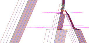
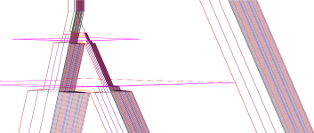
Figure 27 presents the scheme for failure of test on the left. This happens if encounters anything: it is either something that should not be involved and is too closed or just that is not the leftmost macro-signal involved, so that macro-collision has to be aborted to be started by the rightful macro-signal. Since probe signal are not concerned, the signals that can be met on the left are: , , or (for any ).
On meeting, bounces back as . It arrives back to and marks it as . When meets , it is destroyed and is restored; nothing is emitted so that the macro-collision is aborted. The signal has to be disposed of; this is done either on or on .
Figure 28 presents the scheme for failure of test on the right. The alternation of and is not indicated for clarity although they are used to detect failure. The failure might come from some with too small or from meeting , i.e. before is met. In any failure case, (or ) bounces back as . When meets , it is destroyed and is restored; nothing is emitted so that the macro-collision is aborted. The signal has to be disposed, this happens on meeting .
It might happen that the arrives before onto . It might also happen that there is failure on both side and arrival onto can be in any order. The listed rules do take this into account.
The used meta-signals and (failure) collision rules are defined in Figs. 24 and 29. The rules in Figure 29 are divided in three part: fail on left only, fail on right only and additional rules in case fail on both left and right.
, { , } { , } , { , } { , } , { , } { , } , { , } { , } , { , } { } , { , } { } , { , } { } , { , } { } , { , } { , } , { , } { , } , { , } { } , { , } { } , { , } { } , { , } { } , { , } { } , { , } { } , { , } { }
The function can be trivially extended for this section by ignoring all of its signals, as they don’t affect the identity of macro-signals. Again, the number of additional signals accounted for by this section for one collision is bounded, therefore is indeed defined locally.
5.3 Check Participating Signals
From this point, it is known that the index of involved macro-signals ranges from to (included). But it is not known whether they actually participate in one single macro-collision (the situations in Fig. 2 are not yet distinguished).
To check this, the two first ( and ) are used to organise meeting points with the all potential (). If any appear anywhere except at their assigned meeting point, then it is known that it will not pass where and intersect (and the macro-collision aborts). The meeting points are computed according to the speeds (like in Fig. 22). This constructions is presented on Fig. 30 with potential dashed. The equation (1) is used again to compute the intersection points and to deduce the speeds.
Signal and slower signal go on the right. If the first meets is , then there are only two macro-signals involved, it disappears and lets starts the next stage.
Otherwise, turns to which crosses the configuration until it meets or a mismatch. cross at and branches into several . Each time meets some , then there should also be the corresponding . And the resolution is started.
If any is met with the wrong () or without any, turns into . This latter cancels all remaining and disappears with . The resolution is not started.
The used meta-signals and collision rules are defined in Figs. 31 and 32. The speed of has to be fast enough so that occurs before intersects any . The position of and of such intersections are again obtained using (1), yielding the necessary speeds of the signals .
Once again, simply ignores the new meta-signals and collisions, which are in bounded amount for each collision.
Altogether, the devices presented in this section yield the following lemma, which states that U correctly simulates one collision from clean inputs.
Lemma 10.
Let be a collision rule of , and let be a configuration of whose signals are exactly and the positions of these signals are such that they all meet at some point . Let be the associated space-time diagram.
Let be a configuration such that , and which is clean at every position of a signal in . Then there is a and such that is a -checked configuration for .
Parameter Value = , = = = Meta-signal speed , , , , ,
, { , } { } , { , } { , } , { , } { , } , { , } { } { } , { , } { } , { , , } { , } , { , , } { , } , { , } { , } , { , , } { , } , { , } { } , { , } { } , { , } { }
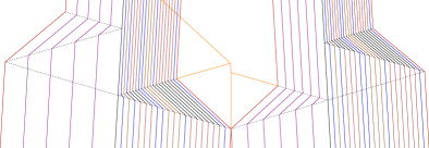
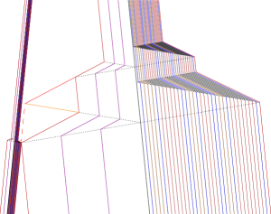
6 Simulation Examples
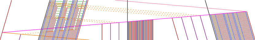
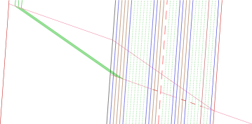
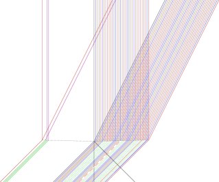
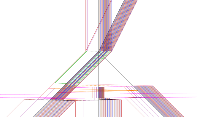
The presented construction works and has been implemented. It has been entirely programmed in an ad hoc language for signal machines. Given a signal machine, the library generate the corresponding together with a function to translate initial configurations. This has been used to generate all the pictures. Figure 33 presents a simulation of the dynamics in Fig. 1(a).
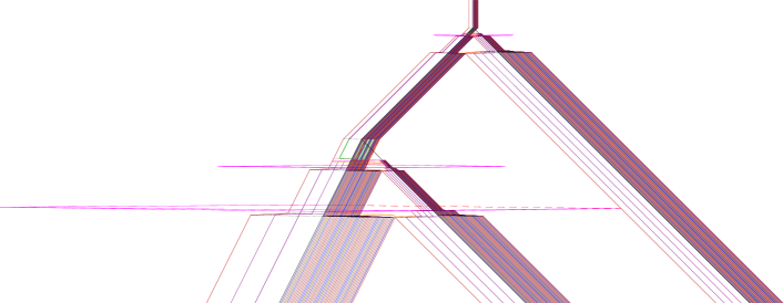
Figure 34 provides different test and check failures before resolving the correct macro-collisions as well as a 3 macro-signal collision.
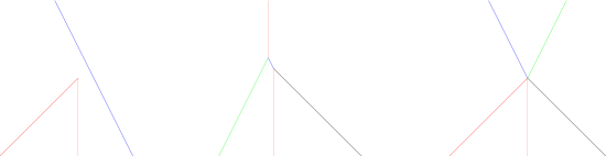
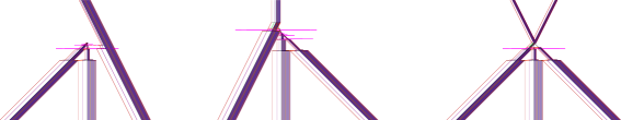
Figure 35 represents a space-time diagram with finitely many collisions with no special regularity.
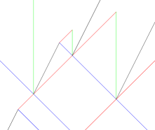
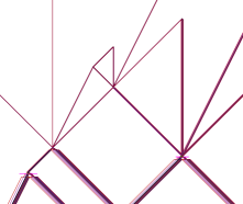
Figure 36 represents a space-time diagram with a simple accumulation on top and its simulation.
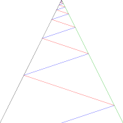
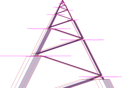
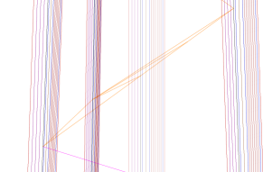
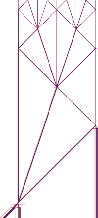
Figure 37 is the basis for firing squad synchronisation on Cellular Automaton. On signal machines, since space and time are continuous, it generates a fractal. The simulation contains more than 100,000 signals. It has been use as a test for robustness.

7 Conclusion
Altogether, the construction proves the following result.
Theorem 11.
For any finite set of real numbers , there is a -universal signal machine. The set of where ranges over finite sets of real numbers is an intrinsically universal family of signal machines.
With the definition of simulation used, there does not exist any intrinsically universal signal machine since having a signal exactly located where the simulated signals implies that the speed of the simulated signal must be available, but every signal machine has finitely many speeds. On the other hand, it might work with some other reasonable definition of simulation, maybe considering some kind of approximation.
Signal machine may produce accumulations (infinitely many collisions in a bounded part of the space-time). The simulation works up to the first accumulation (excluded) where the configuration of the simulated machine cease to be defined in Figure 37.
Using macro-signals forces to deal with width. Hopefully, macro-signals can be made as thin as needed. Nevertheless, as seen through the paper, it requires a lot of technicalities to deal with that.
In the construction, each macro-signals carries the list of rules associates with it, thus its dynamics, like a cell carries its DNA. We wonder what might happen and what kind of artefact could be created if some way to dynamically modify the table were introduced.
References
- Adamatzky (2002) Andrew Adamatzky, editor. Collision based computing. Springer, 2002.
- Albert and Čulik II (1987) Jürgen Albert and Karel Čulik II. A Simple Universal Cellular Automaton and its One-Way and Totalistic Version. Complex Systems, 1:1–16, 1987.
- Arrigh and Grattage (2012) Pablo Arrigh and Jonathan Grattage. Partitioned quantum cellular automata are intrinsically universal. Natural Computing, 11(1):13–22, 2012. doi: 10.1007/s11047-011-9277-6.
- Blum et al. (1989) Lenore Blum, Michael Shub, and Steve Smale. On a Theory of Computation and Complexity over the Real Numbers: NP-Completeness, Recursive Functions and Universal Machines. Bull Amer Math Soc, 21(1):1–46, 1989.
- Boccara et al. (1991) Nino Boccara, J. Nasser, and Michel Roger. Particle-like structures and interactions in spatio-temporal patterns generated by one-dimensional deterministic cellular automaton rules. Phys. Rev. A, 44(2):866–875, 1991.
- Cook (2004) Matthew Cook. Universality in elementary cellular automata. Complex Systems, 15:1–40, 2004.
- Delorme and Mazoyer (2002) Marianne Delorme and Jacques Mazoyer. Signals on cellular automata. In Andrew Adamatzky, editor, Collision-based computing, pages 234–275. Springer, 2002.
- Doty et al. (2010) David Doty, Jack H. Lutz, Matthew J. Patitz, Scott M. Summers, and Damien Woods. Intrinsic Universality in Self-Assembly. In Jean-Yves Marion and Thomas Schwentick, editors, 27th Int. Symposium on Theoretical Aspects of Computer Science, (STACS 2010), Nancy, France, volume 5 of LIPIcs, pages 275–286. Schloss Dagstuhl-Leibniz-Zentrum fuer Informatik, 2010. doi: 10.4230/LIPIcs.STACS.2010.2461.
- Doty et al. (2012) David Doty, Jack H. Lutz, Matthew J. Patitz, Robert T. Schweller, Scott M. Summers, and Damien Woods. The tile assembly model is intrinsically universal. In 53rd Annual IEEE Symposium on Foundations of Computer Science, FOCS 2012, New Brunswick, NJ, USA, October, 2012, pages 302–310. IEEE Computer Society, 2012. ISBN 978-1-4673-4383-1. doi: 10.1109/FOCS.2012.76.
- Durand-Lose (1995) Jérôme Durand-Lose. Reversible Cellular Automaton Able to Simulate Any Other Reversible One Using Partitioning Automata. In LATIN 1995, number 911 in LNCS, pages 230–244. Springer, 1995. doi: 10.1007/3-540-59175-3˙92.
- Durand-Lose (2006) Jérôme Durand-Lose. Abstract geometrical computation 1: Embedding black hole computations with rational numbers. Fund Inf, 74(4):491–510, 2006.
- Durand-Lose (2007) Jérôme Durand-Lose. Abstract Geometrical Computation and the Linear Blum, Shub and Smale Model. In Barry S. Cooper, Benedikt. Löwe, and Andrea Sorbi, editors, Computation and Logic in the Real World, 3rd Conf. Computability in Europe (CiE 2007), number 4497 in LNCS, pages 238–247. Springer, 2007. doi: 10.1007/978-3-540-73001-9˙25.
- Durand-Lose (2008) Jérôme Durand-Lose. The Signal Point of View: From Cellular Automata to Signal Machines. In Bruno Durand, editor, Journées Automates cellulaires (JAC ’08), pages 238–249, 2008.
- Durand-Lose (2009) Jérôme Durand-Lose. Abstract geometrical computation 3: Black holes for classical and analog computing. Nat Comput, 8(3):455–472, 2009. doi: 10.1007/s11047-009-9117-0.
- Durand-Lose (2012) Jérôme Durand-Lose. Abstract Geometrical Computation 6: a Reversible, Conservative and Rational Based Model for Black Hole Computation. Int J Unconventional Computing, 8(1):33–46, 2012.
- Goles Ch. et al. (2011) Eric Goles Ch., Pierre-Etienne Meunier, Ivan Rapaport, and Guillaume Theyssier. Communication Complexity and Intrinsic Universality in Cellular Automata. Theor. Comput. Sci., 412(1-2):2–21, 2011. doi: 10.1016/j.tcs.2010.10.005.
- Hordijk et al. (1998) Wim Hordijk, James P. Crutchfield, and Melanie Mitchell. Mechanisms of emergent computation in cellular automata. In A. E. Eiben, Thomas Bäck, Marc Schoenauer, and Hans-Paul Schwefel, editors, Parallel Problem Solving from Nature - PPSN V, 5th Int. Conf., Amsterdam, The Netherlands, volume 1498 of LNCS, pages 613–622. Springer, 1998. doi: 10.1007/BFb0056903.
- Jakubowski et al. (1996) Mariusz H. Jakubowski, Kenneth Steiglitz, and Richard K. Squier. When can solitons compute? Complex Systems, 10(1), 1996.
- Jakubowski et al. (2000) Mariusz H. Jakubowski, Kenneth Steiglitz, and Richard K. Squier. Information transfer between solitary waves in the saturable schrödinger equation. In Proceedings from the International Conference on Complex Systems on Unifying Themes in Complex Systems, pages 281–293, Cambridge, MA, USA, 2000. Perseus Books. ISBN 0-7382-0049-2. URL http://dl.acm.org/citation.cfm?id=331767.331919.
- Jakubowski et al. (2017) Mariusz H. Jakubowski, Kenneth Steiglitz, and Richard K. Squier. Computing with classical soliton collisions. In Andrew Adamatzky, editor, Advances in Unconventional Computing vol. 2: Prototypes, Models and Algorithms, volume 23 of Emergence, Complexity and Computation, pages 261–295. Springer, 2017. doi: 10.1007/978-3-319-33921-4˙12.
- Jin and Chen (2016) Weifeng Jin and Fangyue Chen. Symbolic dynamics of glider guns for some one-dimensional cellular automata. Nonlinear Dynamics, 86(2):941–952, Oct 2016. ISSN 1573-269X. doi: 10.1007/s11071-016-2935-6.
- Lindgren and Nordahl (1990) Kristian Lindgren and Mats G. Nordahl. Universal computation in simple one-dimensional cellular automata. Complex Systems, 4:299–318, 1990.
- Martiel and Martin (2015) Simon Martiel and Bruno Martin. An Intrinsically Universal Family of Causal Graph Dynamics. In Jérôme Durand-Lose and Benedek Nagy, editors, Machines, Computations, and Universality - 7th Int. Conf., Famagusta, North Cyprus, (MCU 2015), volume 9288 of LNCS, pages 129–148. Springer, 2015. doi: 10.1007/978-3-319-23111-2˙9.
- Mazoyer and Rapaport (1998) Jacques Mazoyer and Ivan Rapaport. Inducing an Order on Cellular Automata by a Grouping Operation. In 15th Annual Symposium on Theoretical Aspects of Computer Science (STACS 1998), number 1373 in LNCS, pages 116–127. Springer, 1998.
- Mazoyer and Terrier (1999) Jacques Mazoyer and Véronique Terrier. Signals in one-dimensional cellular automata. Theoret Comp Sci, 217(1):53–80, 1999. doi: 10.1016/S0304-3975(98)00150-9.
- Meunier et al. (2014) Pierre-Etienne Meunier, Matthew J. Patitz, Scott M. Summers, Guillaume Theyssier, Andrew Winslow, and Damien Woods. Intrinsic Universality in Tile Self-Assembly Requires Cooperation. In Chandra Chekuri, editor, 25th Annual ACM-SIAM Symposium on Discrete Algorithms, SODA 2014, Portland, Oregon, USA, pages 752–771. SIAM, 2014. doi: 10.1137/1.9781611973402.56.
- Mitchell (1996) Melanie Mitchell. Computation in Cellular Automata: a Selected Review. In T. Gramss, S. Bornholdt, M. Gross, M. Mitchell, and T. Pellizzari, editors, Nonstandard Computation, pages 95–140. Weinheim: VCH Verlagsgesellschaft, 1996.
- Ollinger (2001) Nicolas Ollinger. Two-States Bilinear Intrinsically Universal Cellular Automata. In Fundamentals of Computation Theory, 13th International Symposium (FCT 2001), number 2138 in LNCS, pages 369–399. Springer, 2001.
- Ollinger (2003) Nicolas Ollinger. The Intrinsic Universality Problem of One-Dimensional Cellular Automata. In 20th Annual Symposium on Theoretical Aspects of Computer Science (STACS 2003), number 2607 in LNCS, pages 632–641. Springer, 2003.
- Siwak (2001) Pawel Siwak. Soliton-like dynamics of filtrons of cycle automata. Inverse Problems, 17:897–918, 2001.
- Varshavsky et al. (1970) Victor I. Varshavsky, Vyacheslav B. Marakhovsky, and V. A. Peschansky. Synchronization of interacting automata. Math System Theory, 4(3):212–230, 1970.
- Woods (2013) Damien Woods. Intrinsic Universality and the Computational Power of Self-Assembly. In Turlough Neary and Matthew Cook, editors, Proceedings Machines, Computations and Universality 2013, MCU 2013, Zürich, Switzerland, volume 128 of EPTCS, pages 16–22, 2013. doi: 10.4204/EPTCS.128.5.
- Yunès (2007) Jean-Baptiste Yunès. Simple new algorithms which solve the firing squad synchronization problem: a 7-states 4n-steps solution. In Jérôme Durand-Lose and Maurice Margenstern, editors, Machine, Computations and Universality (MCU 2007), number 4664 in LNCS, pages 316–324. Springer, 2007.
Extra Material
An archive is available with examples, simulation source and java programs to run it at
http://www.univ-orleans.fr/lifo/Members/Jerome.Durand-Lose/Recherche/AGC_Intrinsic_Univ_SM__FILES.tgz
Figure 38 represents the same initial configuration as Fig. 35, but the speed are times faster. This is used to check that large speeds are handled correctly.
Appendix A Table of Used Symbols
Table of symbols
Symbol Definition Page