On robust stopping times for detecting changes in distribution

Abstract

Let $X_{1},X_{2},\ldots$ be independent random variables observed sequentially and such that $X_{1},\ldots,X_{\theta-1}$ have a common probability density $p_{0}$, while $X_{\theta},X_{\theta+1},\ldots$ are all distributed according to $p_{1}\neq p_{0}$. It is assumed that $p_{0}$ and $p_{1}$ are known, but the time change $\theta\in\mathbb{Z}^{+}$ is unknown and the goal is to construct a stopping time $\tau$ that detects the change-point $\theta$ as soon as possible. The existing approaches to this problem rely essentially on some a priori information about $\theta$. For instance, in Bayes approaches, it is assumed that $\theta$ is a random variable with a known probability distribution. In methods related to hypothesis testing, this a priori information is hidden in the so-called average run length. The main goal in this paper is to construct stopping times which do not make use of a priori information about $\theta$, but have nearly Bayesian detection delays. More precisely, we propose stopping times solving approximately the following problem:

$$\begin{split}&\quad\Delta(\theta;\tau^{\alpha})\rightarrow\min_{\tau^{\alpha}}\quad\textbf{subject to}\quad\alpha(\theta;\tau^{\alpha})\leq\alpha\ \textbf{ for any}\ \theta\geq 1,\end{split}$$

where $\alpha(\theta;\tau)=\mathbf{P}_{\theta}\bigl{\{}\tau<\theta\bigr{\}}$ is the false alarm probability and $\Delta(\theta;\tau)=\mathbf{E}_{\theta}(\tau-\theta)_{+}$ is the average detection delay, and explain why such stopping times are robust w.r.t. a priori information about $\theta$.

Keywords: stopping time, false alarm probability, average detection delay, Bayes stopping time, CUSUM method, multiple hypothesis testing.

2000 Mathematics Subject Classification: Primary 62L10, 62L15; secondary 60G40.

1 Introduction

Let $X_{1},X_{2},\ldots$ be independent random variables observed sequentially. It is assumed $X_{1},\ldots,X_{\theta-1}$ have a common probability density $p_{0}(x),\,x\in\mathbb{R}^{d}$, while $X_{\theta},X_{\theta+1},\ldots$ are all distributed according to a probability density $p_{1}(x)\,x\in\mathbb{R}^{d}$. This paper deals with the simplest change-point detection problem where it is supposed $p_{0}$ and $p_{1}$ are known, but the time change $\theta\in\mathbb{Z}^{+}$ is unknown, and the goal is to construct a stopping time $\tau\in\mathbb{Z}^{+}$ that detects $\theta$ as soon as possible. The existing approaches to this problem rely essentially on some a priori information about $\theta$. For instance, in Bayes approaches, it is assumed that $\theta$ is a random variable with a known probability distribution, see e.g. [12]. In methods related to hypothesis testing, this a priori information is hidden in the so-called average run length, see e.g. [7]. Our main goal in this paper is to construct robust stopping times which do not make use of a priori information about $\theta$, but have detection delays close to Bayes ones.

In order to be more precise, denote by $\mathbf{P}_{\theta}$ the probability distribution of $(X_{1},\ldots,X_{\theta-1},X_{\theta},\ldots)^{\top}$ and by $\mathbf{E}_{\theta}$ the expectation with respect to this measure. In this paper, we characterize $\tau$ with the help of two functions in $\theta$:

• false alarm probability

  $$\alpha(\theta;\tau)=\mathbf{P}_{\theta}\bigl{\{}\tau<\theta\bigr{\}};$$

• average detection delay

  $$\Delta(\theta;\tau)=\mathbf{E}_{\theta}(\tau-\theta)_{+},\quad\text{where}\ (x)_{+}=\max\{0,x\},$$

and our goal is to construct stopping times solving the following problem:

$$\begin{split}&\Delta(\theta;\tau^{\alpha})\rightarrow\min_{\tau^{\alpha}}\quad\textbf{subject to}\quad\alpha(\theta;\tau^{\alpha})\leq\alpha\quad\textbf{for any}\quad\theta\geq 1.\end{split}$$ (1)

The main difficulty in this problem is related to the fact that for a given stopping time $\tau^{\alpha}$ the average delay $\Delta(\theta;\tau^{\alpha})$ depends on $\theta$. This means that in order to compare two stopping times $\tau_{1}^{\alpha}$ and $\tau_{2}^{\alpha}$, one has to compare two functions in $\theta\in\mathbb{Z}^{+}$. Obviously, this is not feasible from a mathematical viewpoint and the principal objective in this paper is to propose stopping times providing good approximative solutions to (1). Notice also here that similar problems are common and well-known in statistics and there are reasonable approaches to obtain their solutions.

In change-point detection, there are two standard methods for constructing stopping times.

• A Bayes approach. The first Bayes change detection problem was stated in [4] for on-line quality control problem for continuous technological processes. In detecting changes in distributions this approach assumes that $\theta$ is a random variable with a known distribution

  $$\pi_{m}=\mathbf{P}\{\theta=m\},\quad m=1,2,\ldots,$$

  and the goal is to construct a stopping time $\tau_{\pi}^{\alpha}$ that solves the averaged version of (1), i.e.,

  $$\begin{split}&\sum_{m=1}^{\infty}\pi_{m}\Delta(m;\tau_{\pi}^{\alpha})\rightarrow\min_{\tau_{\pi}^{\alpha}}\quad\textbf{subject to}\quad\sum_{m=1}^{\infty}\pi_{m}\alpha(m;\tau_{\pi}^{\alpha})\leq\alpha.\end{split}$$ (2)

  Emphasize that in contrast to (1), this problem is well defined from a mathematical viewpoint, but its solution depends on a priori law $\pi$.

• A hypothesis testing approach. The first non-Bayesian change detection algorithm based on sequential hypothesis testing was proposed in [7]. Denote by $X^{n}=(X_{1},\ldots,X_{n})^{\top}$ the observations till moment $n$. The main idea in this approach is to test sequentially

  $$\begin{split}&\textsl{simple hypothesis }\\ &{\rm H}_{0}^{n}:X^{n}\sim\prod_{i=1}^{n}{p}_{0}(x_{i})\\ &\textsl{vs. compound alternative}\\ &{\rm H}_{1}^{n}:X^{n}\sim\prod_{i=1}^{m-1}{p}_{0}(x_{i})\prod_{i=m}^{n}{p}_{1}(x_{i}),\quad m\leq n.\end{split}$$ (3)

  So, stopping time $\tau$ is defined as follows:

  • if ${\rm H}_{0}^{n}$ is accepted, the observations are continued, i.e., we test ${\rm H}_{0}^{n+1}$ vs. ${\rm H}_{1}^{n+1}$;

  • If ${\rm H}_{1}^{n}$ is accepted, then we stop and $\tau=n$.

In order to motivate our idea of robust stopping times, we discuss very briefly basic statistical properties of the above mentioned approaches.

1.1 A Bayes approach

Usually in this approach the geometric a priori distribution

$$\pi_{m}=\gamma(1-\gamma)^{m-1},\quad m=1,2,\ldots,\quad\gamma>0,$$

is used. Positive parameter $\gamma$ is assumed to be known. In this case, the optimal stopping time is given by the following famous theorem [12]:

Theorem 1.1.

The optimal Bayes stopping time (see (2)) is given by

$$\tau_{\gamma}^{\alpha}=\min\{k:\bar{\pi}(X^{k})\geq 1-\alpha_{\gamma}\},$$ (4)

where

$$\bar{\pi}_{\gamma}(X^{k})=\mathbf{P}\bigl{\{}\theta\leq k|X^{k}\bigr{\}},$$

and $\alpha_{\gamma}\approx\alpha$ is a constant.

Notice that the geometric a priori distribution results in the following recursive formula for a posteriori probability (see, e.g., [12]):

$$\begin{split}&\bar{\pi}_{\gamma}(X^{k})=\\ &\quad=\frac{[\gamma+(1-\gamma)\bar{\pi}_{\gamma}(X^{k-1})]p_{1}(X_{k})}{[\gamma+(1-\gamma)\bar{\pi}_{\gamma}(X^{k-1})]p_{1}(X_{k})+[1-\bar{\pi}_{\gamma}(X^{k-1})](1-\gamma)p_{0}(X_{k})}.\end{split}$$ (5)

So, if we denote for brevity

$$\rho_{\gamma}(X^{k})=\frac{\bar{\pi}_{\gamma}(X^{k})}{1-\bar{\pi}_{\gamma}(X^{k})},$$

then (5) may be rewritten in the following equivalent form:

$$\rho_{\gamma}(X^{k})=\frac{\gamma+\rho_{\gamma}(X^{k-1})}{1-\gamma}\times\frac{p_{1}(X_{k})}{p_{0}(X_{k})}.$$ (6)

From this equation we see, in particular, that the Bayes stopping time depends on $\gamma$ that is hardly known in practice. In statistics, in order to avoid such dependence, the uniform a priori distribution is usually used. Let’s look how this idea works in change point detection. The uniform a priori distribution assumes that $\gamma=0$ and in this case we obtain immediately from (6)

$$\begin{split}\rho_{0}(X^{k})=\rho_{0}(X^{k-1})\times\frac{p_{1}(X_{k})}{p_{0}(X_{k})}.\end{split}$$

Therefore, for

$$L_{0}(X^{k})=\log[\rho_{0}(X^{k})],$$

we get

$$L_{0}(X^{k})=\sum_{i=1}^{k}\log\frac{p_{1}(X_{i})}{p_{0}(X_{i})}.$$

Hence, the optimal stopping time in the case of the uniform a priori distribution is given by

$$\tau^{\alpha}_{\circ}=\min\bigl{\{}k:L_{0}(X^{k})\geq t^{\alpha}\bigr{\}},$$ (7)

where $t^{\alpha}$ is some constant. Fig. 1 shows a typical trajectory of $L_{0}(X^{k}),\,k=1,2,\ldots$, in detecting change in the Gaussian distribution with $\theta=80$.

Computing the false alarm probability for this stopping time is not difficult and based on the following simple fact. Let

$$\phi(\lambda)=\mathbf{E}_{\infty}\exp\biggl{[}\lambda\log\frac{p_{1}(X_{1})}{p_{0}(X_{1})}\biggr{]}.$$

Lemma 1.1.

For any $\lambda>0$

$$\mathbf{E}_{\infty}\exp\bigl{\{}-\tau_{\circ}^{\alpha}\log[\phi(\lambda)]\bigr{\}}\mathbf{1}\bigl{(}\tau_{\circ}^{\alpha}<\infty\bigr{)}\leq\exp(-\lambda t^{\alpha}).$$

It follows immediately from the definition of $\phi(\lambda)$ that if $\lambda=1$, then $\phi(\lambda)=1$. So, by this Lemma we get

$$\mathbf{P}_{\infty}\bigl{\{}\tau_{\circ}^{\alpha}<\infty\bigr{\}}\leq\exp(-t^{\alpha}).$$

As to the average detection delay, it can be easily computed with the help of the famous Wald identity [14, 2]. The next theorem summarizes principal properties of $\tau^{\alpha}_{\circ}$. Let us assume that

$$\mu_{0}\stackrel{{\scriptstyle\rm def}}{{=}}\int\log\frac{p_{0}(x)}{p_{1}(x)}p_{0}(x)\,dx>0\quad\text{and}\quad\mu_{1}\stackrel{{\scriptstyle\rm def}}{{=}}\int\log\frac{p_{1}(x)}{p_{0}(x)}p_{1}(x)\,dx>0.$$

Theorem 1.2.

Let $t^{\alpha}=\log(1/\alpha).$ Then for $\tau_{\circ}^{\alpha}$ defined by (7) we have

$$\alpha(\theta;\tau_{\circ}^{\alpha})\leq\alpha,$$

$$\Delta(\theta;\tau_{\circ}^{\alpha})=\frac{\log(1/\alpha)+\theta\mu_{0}}{\mu_{1}}.$$

Fig. 1 illustrates this theorem showing $L_{0}(X^{k}),\,k=1,\ldots,200$, in the case of the change in the mean of the Gaussian distribution with $\theta=80$.

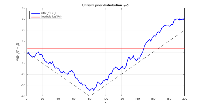
Figure 1: Detecting change in the mean of Gaussian distribution with the help of $\tau^{\alpha}_{\circ}$.

We would like to emphasize that the fact that $\Delta(\theta;\tau_{\circ}^{\alpha})$ is linear in $\theta$ is not good from practical and theoretical viewpoints. In order to understand why it is so, let us now turn back to the Bayes setting assuming that $\gamma>0$. In this case the following theorem holds true.

Theorem 1.3.

Suppose $\gamma>0$. Then for $\tau^{\alpha}_{\gamma}$ defined by (4) we have

$$\max_{\theta\in\mathbb{Z}^{+}}\alpha(\theta;\tau_{\gamma}^{\alpha})=1,$$

$$\Delta(\theta;\tau_{\gamma}^{\alpha})=\frac{\log[1/(\gamma\alpha)]}{\mu_{1}}+O(1),\quad\text{as}\quad\gamma,\alpha\rightarrow 0.$$ (8)

This theorem may be proved with the help of the standard techniques described, e.g., in [1].

Fig. 2 illustrates typical behavior of $\log[\rho_{\gamma}(X^{k})]$ with $\gamma>0$. Notice that if $\tau_{\circ}^{\alpha}$ is used in the considered case, then we obtain by (8)

$$\mathbf{E}\Delta(\theta;\tau_{\circ}^{\alpha})=\frac{\log(1/\alpha)}{\mu_{1}}+\frac{\mu_{0}}{\mu_{1}}\times\frac{1}{\gamma}.$$

So, we see that this mean detection delay is far away from the optimal Bayes one given by

$$\mathbf{E}\Delta(\theta;\tau_{\gamma}^{\alpha})=\frac{\log(1/\alpha)}{\mu_{1}}+\frac{1}{\mu_{1}}\times\log{\frac{1}{\gamma}}+O(1),\quad\text{as}\quad\gamma,\alpha\rightarrow 0.$$

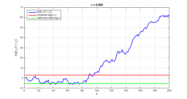
Figure 2: Detecting change in the mean of Gaussian distribution with the help of $\tau^{\alpha}_{\gamma}$ ($\gamma=0.005$).

Let us now summarize briefly main facts related to the classical Bayes approach.

• if $\gamma=0$, then the average detection delay of the Bayes stopping time grows linearly in $\theta$;

• when $\gamma>0$, the maximal false alarm probability is not controlled.

In view of these facts it is clear that the standard Bayes technique cannot provide reasonable solutions to (1).

1.2 A hypothesis testing approach

The idea of this approach is based on the well-known sequential testing of two simple hypothesis [15]. However, we would like to emphasize that in contrast to the standard setting in [15], in the change-point detection, this approach has a rather heuristic character since here we test a simple hypothesis versus a compound alternative whose complexity grows with the observations volume.

In sequential hypothesis testing there are two common methods

• maximum likelihood;

• Bayesian.

The maximum likelihood test accepts hypothesis ${\rm H}_{1}^{n}$ (see (3)) when

$$\max_{k\leq n}\frac{\prod_{i=1}^{k-1}p_{0}(X_{i})\prod_{i=k}^{n}p_{1}(X_{i})}{\prod_{i=1}^{n}p_{0}(X_{i})}\geq t^{\alpha}$$

or, equivalently,

$$M(X^{n})\geq t^{\alpha},$$

where

$$M(X^{n})=\max_{k\leq n}\sum_{i=k}^{n}\log\frac{p_{1}(X_{i})}{p_{0}(X_{i})}.$$

The threshold $t^{\alpha}$ is computed as follows

$$t^{\alpha}=\min\Bigl{\{}t:\mathbf{P}_{\infty}\bigl{\{}M(X^{n})\geq t\bigr{\}}\leq\alpha\Bigr{\}},$$

where $\alpha$ is the first type error probability. Notice that by Lemma 1.1

$$\mathbf{P}_{\infty}\bigl{\{}M(X^{n})\geq x\bigr{\}}\leq\exp(-x).$$

Therefore the maximum likelihood test results in the following stopping time:

$$\tau_{\rm ml}^{\alpha}=\min\biggl{\{}n:\,M(X^{n})\geq\log\frac{1}{\alpha}\biggr{\}}.$$ (9)

Notice also that $M(X^{n})$ admits a simple recursive computation [7]. Indeed, notice

$$\begin{split}&\max_{k\leq n}\sum_{i=k}^{n}\log\frac{p_{1}(X_{i})}{p_{0}(X_{i})}\\ &\quad=\max\biggl{\{}\log\frac{p_{1}(X_{n})}{p_{0}(X_{n})},\log\frac{p_{1}(X_{n})}{p_{0}(X_{n})}+\max_{k\leq n-1}\sum_{i=k}^{n-1}\log\frac{p_{1}(X_{i})}{p_{0}(X_{i})}\biggr{\}}\\ &\quad=\log\frac{p_{1}(X_{n})}{p_{0}(X_{n})}+\max\biggl{\{}0,\max_{k\leq n-1}\sum_{i=k}^{n-1}\log\frac{p_{1}(X_{i})}{p_{0}(X_{i})}\biggr{\}}.\end{split}$$

Therefore

$$M(X^{n})=\log\frac{p_{1}(X_{n})}{p_{0}(X_{n})}+\bigl{[}M(X^{n-1})\bigr{]}_{+}.$$ (10)

This method is usually called CUSUM algorithm. It is well known that it is optimal in Lorden [5] sense, i.e., for properly chosen $\alpha$, $\tau_{\rm ml}^{\alpha}$ minimizes

$$\sup_{\theta\in\mathbb{Z}^{+}}{\rm ess}\sup\mathbf{E}_{\theta}\bigl{[}(\tau-\theta)_{+}|X_{1},\ldots,X_{\theta-1}\bigr{]}$$

in the class of stopping times $\bigl{\{}\tau:\mathbf{E}_{\infty}\tau\geq T\bigr{\}}$, see [6].

However, with this method cannot control the false alarm probability as shows the following theorem.

Theorem 1.4.

For any $\alpha\in(0,1)$

$$\max_{\theta\in\mathbb{Z}^{+}}\alpha(\theta;\tau_{\rm ml}^{\alpha})=1.$$

As $\alpha\rightarrow 0$

$$\Delta(\theta;\tau_{\rm ml}^{\alpha})=\frac{1+o(1)}{\mu_{1}}\log\frac{1}{\alpha}.$$

The Bayesian test is based on the assumption that $\theta$ is uniformly distributed on $[1,n]$. So, this test accepts ${\rm H}_{1}^{n}$ when

$$S(X^{n})\stackrel{{\scriptstyle\rm def}}{{=}}\sum_{k=1}^{n}\frac{\prod_{i=1}^{k-1}p_{0}(X_{i})\prod_{i=k}^{n}p_{1}(X_{i})}{\prod_{i=1}^{n}p_{0}(X_{i})}\geq t^{\alpha}.$$ (11)

Since

$$S(X^{n})=\sum_{k=1}^{n}\prod_{i=k}^{n}\frac{p_{1}(X_{i})}{p_{0}(X_{i})},$$

and

$$\begin{split}\sum_{k=1}^{n}\prod_{i=k}^{n}\frac{p_{1}(X_{i})}{p_{0}(X_{i})}&=\sum_{k=1}^{n-1}\prod_{i=k}^{n}\frac{p_{1}(X_{i})}{p_{0}(X_{i})}+\frac{p_{1}(X_{n})}{p_{0}(X_{n})}\\ &=\biggl{[}1+\sum_{k=1}^{n-1}\prod_{i=k}^{n-1}\frac{p_{1}(X_{i})}{p_{0}(X_{i})}\biggr{]}\frac{p_{1}(X_{n})}{p_{0}(X_{n})},\end{split}$$

the test statistics in (11) admits the following recursive computation:

$$S(X^{n})=\bigl{[}1+S(X^{n-1})\bigr{]}\times\frac{p_{1}(X_{n})}{p_{0}(X_{n})}.$$

So, the corresponding stopping time is given by

$$\tau_{\rm S}^{\alpha}=\min\bigl{\{}k:S(X^{k})\geq t^{\alpha}\bigr{\}}.$$

In the literature, this method is known as Shirayev-Roberts (SR) algorithm. It was firstly proposed in [11] and [10]. In [8] and [3] it was shown that it minimizes the integral average delay

$$\frac{1}{\mathbf{E}_{\infty}\tau}\sum_{\theta=1}^{\infty}\mathbf{E}_{\theta}(\tau-\theta)_{+}$$

over all stopping times $\tau$ with $\mathbf{E}_{\infty}\tau\geq T.$ More detailed statistical properties of SR procedure can be found in [9].

As one can see on Fig. 3, in practice, there is no significant difference between CUSUM and SR algorithms.

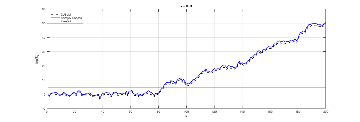
Figure 3: Detecting change in the mean of Gaussian distribution with the help of CUSUM and SR procedures.

Notice also that for SR method the fact similar to Theorem 1.4 holds true. So, the standard hypothesis testing methods results in stopping times with uncontrollable false alarm probabilities.

2 Robust stopping times

The main idea in this paper is to make use of multiple hypothesis testing methods for constructing stopping times. This can be done very easily by replacing the constant threshold in the ML test (9) by one depending on $k$. So, we define the stopping time

$$\widetilde{\tau}^{\alpha}=\min\bigl{\{}k:\,M(X^{k})\geq t^{\alpha}(k)\bigr{\}}.$$

In order to control the false alarm probability and to obtain a nearly minimal average detection delay, we are looking for a minimal function $t^{\alpha}(k),\ k=1,2,\ldots$, such that

$$\mathbf{P}_{\infty}\bigl{\{}\max_{k\geq\mathbb{Z}^{+}}\bigl{[}M(X^{k})-t^{\alpha}(k)\bigr{]}\geq 0\bigr{\}}\leq\alpha.$$

We begin our construction of $t^{\alpha}(k)$ with the following function:

$$\varphi(x)=1+\log(x),\quad x\in\mathbb{R}^{+},$$

and define $m$-iterated $\varphi(\cdot)$ by

$$\Phi_{m}(x)=\varphi\bigl{[}\Phi_{m-1}(x)\bigr{]},\ \text{with}\ \Phi_{1}(x)=\varphi(x).$$

Next, for given $\epsilon\in(0,1)$, define

$$b_{m,\epsilon}(x)=-\log\bigg{[}\frac{1}{\epsilon\Phi^{\epsilon}_{m}(x)}-\frac{1}{\epsilon\Phi^{\epsilon}_{m}(x+1)}\biggr{]},\quad x\in\mathbb{R}^{+}.$$ (12)

Consider the following random variable:

$$\zeta_{m,\epsilon}=\max_{k\in\mathbb{Z}^{+}}\bigl{\{}M(X^{k})-b_{m,\epsilon}(k)\bigr{\}}.$$

The next theorem plays a cornerstone role in our construction of robust stopping times.

Theorem 2.1.

For any $\epsilon\in(0,1)$, $m\geq 1$, and $x>-\log(1-0.2075/2)\approx 0.11$

$$\mathbf{P}\bigl{\{}\zeta_{m,\epsilon}\geq x\bigr{\}}\leq 1-\exp\bigl{\{}-{\rm e}^{-x}\bigl{[}\epsilon^{-1}+{\rm e}^{-x}\bigr{]}\bigr{\}}.$$

Therefore we can define the quantile of order $\alpha$ of $\zeta_{m,\epsilon}$ by

$$t^{\alpha}_{m,\epsilon}=\min\bigl{\{}x:\mathbf{P}\bigl{\{}\zeta_{m,\epsilon}\geq x\bigr{\}}\leq\alpha\bigr{\}}.$$

Fig. 4 shows the distribution functions and quantiles of $\zeta_{1,\epsilon}$ for $\epsilon=\{0.01,0.2,1\}$ computed with the help of Monte-Carlo method.

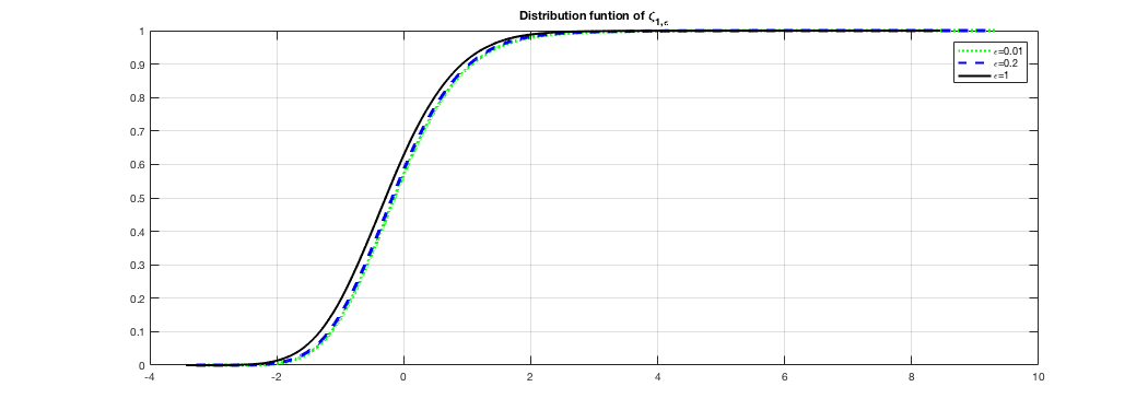
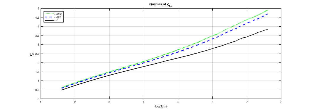
Figure 4: Distribution functions and quantiles of $\zeta_{1,\epsilon}$.

The next theorem describes principal properties of the stopping time

$$\widetilde{\tau}^{\alpha}_{m,\epsilon}=\min\bigl{\{}k:M(X^{k})\geq b_{m,\epsilon}(k)+t^{\alpha}_{m,\epsilon}\bigr{\}}.$$

Theorem 2.2.

For any $\epsilon\in(0,1]$

$$\begin{split}&\alpha\bigl{(}\theta;\widetilde{\tau}^{\alpha}_{m,\epsilon}\bigr{)}\leq\alpha,\\ &\Delta\bigl{(}\theta;\widetilde{\tau}^{\alpha}_{m,\epsilon}\bigr{)}\leq d^{\alpha}_{m,\epsilon}(\theta),\end{split}$$

where $d^{\alpha}_{m,\epsilon}(\theta)$ is a solution to

$$\mu_{1}d^{\alpha}_{m,\epsilon}(\theta)=b_{m,\epsilon}\bigl{[}\theta+d^{\alpha}_{m,\epsilon}(\theta)\bigr{]}+t^{\alpha}_{m,\epsilon}.$$ (13)

The asymptotic behavior of the average delay is described by the following theorem

Theorem 2.3.

For any $\epsilon\in(0,1]$, as ${\alpha}\rightarrow 0$ and $\theta\rightarrow\infty$

$$\Delta\bigl{(}\theta;\widetilde{\tau}_{m,\epsilon}^{\alpha}\bigr{)}\leq\frac{1}{\mu_{1}}\biggl{\{}\log\frac{\theta}{\alpha}+\sum_{j=1}^{m}\log[\Phi_{j}(\theta)]+\epsilon\log[\Phi_{m}(\theta)]+\log\frac{1}{\epsilon}\biggr{\}}+o(1).$$ (14)

Remark. It is easy to check with a simple algebra that for any given $\theta>1$

$$\lim_{j\rightarrow\infty}j\log[\Phi_{j}(\theta)]=2.$$

The robustness of $\widetilde{\tau}_{m,\epsilon}^{\alpha}$ w.r.t. a priori geometric distribution of $\theta$ follows now almost immediately from (14). Indeed, suppose $\theta$ is a random variable with

$$\mathbf{P}\bigl{\{}\theta=k\bigr{\}}=\gamma(1-\gamma)^{k-1},\quad k\in\mathbb{Z}^{+}.$$

Then, averaging (14) w.r.t. this distribution, we obtain

$$\mathbf{E}\Delta\bigl{(}\theta;\widetilde{\tau}_{m,\epsilon}^{\alpha}\bigr{)}\leq\frac{1}{\mu_{1}}\biggl{\{}\log\frac{1}{\alpha\gamma}+\sum_{j=1}^{m}\log\biggl{[}\Phi_{j}\biggl{(}\frac{1}{\gamma}\biggr{)}\biggr{]}+\epsilon\log\biggl{[}\Phi_{m}\biggl{(}\frac{1}{\gamma}\biggr{)}\biggr{]}+\log\frac{1}{\epsilon}\biggr{\}}+o(1)$$

as $\alpha,\gamma\rightarrow 0$, and with (8) we arrive at

Theorem 2.4.

As $\alpha,\gamma\rightarrow 0$

$$\begin{split}\mathbf{E}\Delta\bigl{(}\theta;\widetilde{\tau}_{m,\epsilon}^{\alpha}\bigr{)}\leq&\mathbf{E}\Delta\bigl{(}\theta;\tau_{\gamma}^{\alpha}\bigr{)}+\frac{1}{\mu_{1}}\biggl{\{}\sum_{j=1}^{m}\log\biggl{[}\Phi_{j}\biggl{(}\frac{1}{\gamma}\biggr{)}\biggr{]}+\epsilon\log\biggl{[}\Phi_{m}\biggl{(}\frac{1}{\gamma}\biggr{)}\biggr{]}+\log\frac{1}{\epsilon}\biggr{\}}+O(1)\\ =&(1+o(1))\mathbf{E}\Delta\bigl{(}\theta;\tau_{\gamma}^{\alpha}\bigr{)},\end{split}$$

where $\tau_{\gamma}^{\alpha}$ is the optimal Bayesian stopping time (see Theorem 1.1).

Appendix A Appendix section

Proof of Lemma 1.1.

Since

$$Y_{k}=\exp\bigl{\{}-k\log[\phi(\lambda)]+\lambda L_{0}(X^{k})\bigr{\}}$$

is a martingale with $\mathbf{E}_{\infty}Y_{k}=1$, we have

$$\begin{split}1=&\mathbf{E}_{\infty}Y_{\tau_{\circ}^{\alpha}}=\mathbf{E}_{\infty}Y_{\tau_{\circ}^{\alpha}}\mathbf{1}(\tau_{\circ}^{\alpha}<\infty)+\mathbf{E}_{\infty}Y_{\tau_{\circ}^{\alpha}}\mathbf{1}(\tau_{\circ}^{\alpha}=\infty)\\ \geq&\mathbf{E}_{\infty}Y_{\tau_{\circ}^{\alpha}}\mathbf{1}(\tau_{\circ}^{\alpha}<\infty)=\mathbf{E}_{\infty}\exp\bigl{\{}-\tau_{\circ}^{\alpha}\log[\phi(\lambda)]+\lambda A\bigr{\}}\mathbf{1}(\tau_{\circ}^{\alpha}<\infty).\end{split}$$

∎

In what follows we denote by $e_{k}$ be i.i.d. standard exponential random variables.

Lemma A.1.

For any $m\geq 1$ and $x>-\log(1-0.2075/2)\approx 0.11$

$$\begin{split}\mathbf{P}\Bigl{\{}\max_{k\in\mathbb{Z}^{+}}[e_{k}-b_{m,\epsilon}(k)]\geq x\Bigr{\}}\leq 1-\exp\Bigl{\{}-{\rm e}^{-x}\bigl{[}\epsilon^{-1}+{\rm e}^{-x}\bigr{]}\Bigr{\}},\end{split}$$

where $b_{m,\epsilon}(\cdot)$ is defined by (12).

Proof.

It is easy to check with a simple algebra that for any $u\in[0,1)$

$$\log(1-u)\geq-u-\frac{u^{2}}{2(1-u)}.$$

Therefore with this inequality we obtain

$$\begin{split}&\mathbf{P}\bigl{\{}\max_{k\in\mathbb{Z}^{+}}[e_{k}-b_{m,\epsilon}(k)]\geq x\bigr{\}}=1-\prod_{k=1}^{\infty}\Bigl{\{}1-\mathbf{P}\bigl{\{}e_{k}\geq x+b_{m,\epsilon}(k)\bigr{\}}\Bigr{\}}\\ &\quad=1-\exp\biggl{\{}\sum_{k=1}^{\infty}\log\Bigl{[}1-{\rm e}^{-x-b_{m,\epsilon}(k)}\Bigr{]}\biggr{\}}\\ &\quad\leq 1-\exp\biggl{\{}-{\rm e}^{-x}\sum_{k=1}^{\infty}{\rm e}^{-b_{m,\epsilon}(k)}-\frac{{\rm e}^{-2x}}{2(1-{\rm e}^{-x})}\sum_{k=1}^{\infty}{\rm e}^{-2b_{m,\epsilon}(k)}\biggr{\}}.\end{split}$$ (15)

It follows immediately from the definition of $b_{m,\epsilon}$, see (12), that

$$\sum_{k=1}^{\infty}{\rm e}^{-b_{m,\epsilon}(k)}=\frac{1}{\epsilon\Phi_{m}(1)}=\frac{1}{\epsilon}.$$

It is also easy to check numerically that for any $m\geq 1$ and $\epsilon>0$

$$\sum_{k=1}^{\infty}{\rm e}^{-2b_{m,\epsilon}(k)}<0.2075.$$

Therefore, substituting the above equations in (15), we complete the proof. ∎

Lemma A.2.

For any $x>0$

$$\mathbf{P}_{\infty}\Bigl{\{}\max_{k\in\mathbb{Z}^{+}}[M(X^{k})-b_{m,\epsilon}(k)]\geq x\Bigr{\}}\leq\mathbf{P}\Bigl{\{}\max_{k\in\mathbb{Z}^{+}}[e_{k}-b_{m,\epsilon}(k)]\geq x\Bigr{\}},$$

where random process $M(X^{k})$ is defined by (10).

Proof.

Define random integers $\kappa_{1}<\kappa_{2}<\ldots$ by

$$\kappa_{k}=\min\bigl{\{}s>\kappa_{k-1}:\,M(X^{s})\leq 0\bigr{\}},\quad t_{0}=0,$$

From (10) it is clear that these random variables are renovation points for the random process $M(X^{k})$ and therefore random variables

$$\mu_{k}=\max_{\kappa_{k}<s\leq\kappa_{k+1}}M(X^{s}),\quad k=1,2,\ldots.$$

are independent. Since $b_{m,\epsilon}(k)$ is non-decreasing in $k$ and obviously $\kappa_{k}\geq k$, we get

$$\begin{split}\max_{k\in\mathbb{Z}^{+}}[M(X^{k})-b_{m,\epsilon}(k)]\leq&\max_{k\in\mathbb{Z}^{+}}\max_{{\kappa_{k}<s\leq\kappa_{k+1}}}[M(X^{s})-b_{m,\epsilon}(t_{k})]\\ \leq&\max_{k\in\mathbb{Z}^{+}}[\mu_{k}-b_{m,\epsilon}(k)].\end{split}$$

Therefore, to finish the proof, it suffices to notice that by (10) and Lemma 1.1

$$\mathbf{P}_{\infty}\bigl{\{}\mu_{k}\geq x\bigr{\}}\leq\mathbf{P}_{\infty}\biggl{\{}\max_{k\in\mathbb{Z}^{+}}\sum_{s=\theta}^{k}\log\frac{p_{0}(X_{s})}{p_{1}(X_{s})}\geq x\biggr{\}}\leq\exp(-x).$$

∎

Theorem 2.1 follows now immediately from Lemmas A.1, A.2.

Proof of Theorem 2.2.

It follows from (10) that for all $k\geq\theta$

$$M(X^{k})\geq\sum_{s=\theta}^{k}\log\frac{p_{0}(X_{s})}{p_{1}(X_{s})}$$

and therefore

$$\Delta(\theta;\widetilde{\tau}_{m,\epsilon})\leq\mathbf{E}_{\theta}\tau^{+},$$

where

$$\tau^{+}=\min\biggl{\{}k\geq 1:\sum_{s=\theta}^{\theta+k}\log\frac{p_{0}(X_{s})}{p_{1}(X_{s})}\geq b_{m,\epsilon}(\theta+k)+t^{\alpha}_{m,\epsilon}\biggr{\}}.$$

Computing $\mathbf{E}_{\theta}\tau^{+}$ is based on the famous Wald’s identity [14] (see also [2]). For given $\theta\in\mathbb{Z}^{+},m\in\mathbb{Z}^{+},\epsilon>0$, define function

$$B(k)=b_{m,\epsilon}(\theta+k)+t^{\alpha}_{m,\epsilon},\ k\in\mathbb{Z}^{+}.$$

It is clear that $B(\cdot)$ is a convex function and therefore for any $k_{0}\geq 1$

$$B(k)\leq B(k_{0})+B^{\prime}(x_{0})(k-k_{0}).$$

Hence,

$$\tau^{+}\leq\tau^{++}=\min\biggl{\{}k\geq 1:\sum_{s=\theta}^{\theta+k}\log\frac{p_{0}(X_{s})}{p_{1}(X_{s})}\geq B(k_{0})+B^{\prime}(k_{0})(k-k_{0})\biggr{\}}.$$

Next, we obtain by Wald’s identity

$$\mu_{1}\mathbf{E}_{\theta}\tau^{++}\leq B(k_{0})+B^{\prime}(k_{0})\bigl{(}\mathbf{E}_{\theta}\tau^{++}-k_{0}\bigr{)}$$

and thus

$$\mathbf{E}_{\theta}\tau^{++}\leq\frac{B(k_{0})-B^{\prime}(x_{0})k_{0}}{\mu_{1}-B^{\prime}(k_{0})}.$$ (16)

To finish the proof, we choose $k_{0}=d_{m,\epsilon}^{\alpha}(\theta)$ (see (13)), and notice that $B(k_{0})=\mu_{1}k_{0}$. Hence, by (16)

$$\mathbf{E}_{\theta}\tau^{++}\leq k_{0}=d_{m,\epsilon}^{\alpha}(\theta).$$

∎

Proof of Theorem 2.3.

It follows immediately from Theorem 2.1 that as $\alpha\rightarrow 0$

$$t_{m,\epsilon}^{\alpha}\leq\log\frac{1}{\alpha\epsilon}+o(1).$$ (17)

Next, by convexity of $b_{m,\epsilon}(\cdot)$ we obtain for any $x,x_{0}$

$$b_{m,\epsilon}(\theta+x)\leq b_{m,\epsilon}(\theta+x_{0})+b_{m,\epsilon}^{\prime}(\theta+x_{0})(x-x_{0}).$$

Therefore, choosing

$$x_{0}=\frac{b_{m,\epsilon}(\theta)+t_{m,\epsilon}^{\alpha}}{\mu_{1}}$$

we get by (13)

$$d_{m,\epsilon}^{\alpha}(\theta)\leq\frac{b_{m,\epsilon}(\theta+x_{0})+t_{m,\epsilon}^{\alpha}}{\mu_{1}-b^{\prime}_{m,\epsilon}(\theta+x_{0})}.$$ (18)

So, our next step is to upper bound $b_{m,\epsilon}(\cdot)$. First, notice that

$$-\frac{1}{\epsilon}\frac{d\Phi^{-\epsilon}_{m}(x)}{dx}=\Phi^{-1-\epsilon}_{m}(x)\Phi_{m}^{\prime}(x)=\frac{\Phi^{-\epsilon}_{m}(x)}{x}\prod_{j=1}^{m}\frac{1}{\Phi_{j}(x)},$$

and thus

$$-\log\biggl{[}-\frac{1}{\epsilon}\frac{d\Phi^{-\epsilon}_{m}(x)}{dx}\biggr{]}=\log(x)+\sum_{j=1}^{m}\log[\Phi_{j}(x)]+\epsilon\log[\Phi_{m}(x)].$$

Therefore it follows immediately from this equation and (12) that as $k\rightarrow\infty$

$$b_{m,\epsilon}(k)=\log(k)+\sum_{j=1}^{m}\log[\Phi_{j}(k)]+\epsilon\log[\Phi_{m}(k)]+o(1).$$ (19)

It is also easy to check that

$$b_{m,\epsilon}^{\prime}(k)=O\biggl{(}\frac{1}{k}\biggr{)}.$$ (20)

Finally, substituting (17), (19), and (20) in (18), we complete the proof. ∎

References

- [1] Basseville, M. and Nikiforov, I. V. (1996). Detection of Abrupt Changes: Theory and Application. Prentice-Hall.
- [2] Blackwell, D. (1946). On an equation of Wald, Annals of Math. Stat. 17 84–87.
- [3] Feinberg, E.A. and Shiryaev, A. N. (2006). Quickest detection of drift change for Brownian motion in generalized and Bayesian settings. Statist. Decisions. 24 445–470.
- [4] Girshick M. A. and Rubin, H. (1952). A Bayes approach to a quality control model. Annals Math. Statistics. 23 114–125.
- [5] Lorden, G. (1971). Procedures for reacting to a change in distribution. Ann. Math. Statist. 42 No. 6 1897–1908.
- [6] Moustakides, G. V. (1986). Optimal stopping times for detecting changes in distributions. Ann. of Statist. Vol. 14, No. 4, 1370–1387.
- [7] Page, E. S. (1954). Continuous inspection schemes, Biometrika, 41, 100–115.
- [8] Pollak, M. and Tartakovsky, A. G. (2009). Optimality properties of Shirayev-Roberts procedure. Statist. Sinica, 19, 1729–1739.
- [9] Polunchenko, A. S. and Tartakovsky, A. G. (2010). On optimality of the Shirayev-Roberts procedure for detecting a change in distribution. Annals of Statist., 38, No. 6, 3445–3457.
- [10] Roberts, S.W. (1966). A comparison of some control chart procedures. Technometrics 8, 411–430.
- [11] Shiryaev, A.N. (1961). The problem of the most rapid detection disturbance in a stationary process. Dokl. Math. 2 795–799.
- [12] Shiryaev, A. N. (1978). Optimal Stopping Rules, Springer-Verlag, Berlin, Heidelberg.
- [13] Shiryaev, A. N. (1963). On optimum methods in quickest detection problems. Theory Probab. Appl. 8 22–46.
- [14] Wald, A. (1944). On cumulative sums of random variables. The Annals of Math. Stat. 15 No. 3 283–296.
- [15] Wald, A. (1945). Sequential Tests of Statistical Hypotheses. Annals of Math. Stat. 16 No. 2 117–186.