Abstract

The V-A structure of the weak interactions leads to definite amplitude hierarchies in exclusive heavy-to-light decays mediated by $b\to(d,s)\gamma$ and $b\to(d,s)\ell\bar{\ell}$. However, the extraction of right-handed currents beyond the Standard Model is contaminated by V-A long-distance contributions leaking into right-handed amplitudes. We propose that these quantum-number changing long-distance contributions can be controlled by considering the almost parity-degenerate vector meson final states by exploiting the opposite relative sign of left- versus right-handed amplitudes. For example, measuring the time-dependent rates of a pair of vector $V(J^{P}=1^{-})$ and axial $A(1^{+})$ mesons in $B\to(V,A)\gamma$, up to an order of magnitude is gained on the theory uncertainty prediction, controlled by long-distance ratios to the right-handed amplitude. This renders these decays clean probes to null tests, from the theory side.

1 Introduction

It is well-known that the V-A structure of the weak interaction leaves characteristic traces in the polarisation of weak decays e.g. [1, 2, 3]. This is particularly attractive in heavy-to-light flavour-changing neutral currents, such as $b\to D\gamma$ or $b\to D\ell\bar{\ell}$ with $D=d,s$ and $\ell=e,\mu,\tau$. These transitions therefore make excellent probes to search for new physics with V+A structure, referred to as right-handed currents (RHC) below. Schematically, the effective Hamiltonian for such decays reads

$$H_{\textrm{eff}}^{b\to d\gamma}\sim C\,\bar{d}_{L}\Gamma b\,O_{r}+C^{\prime}\,\bar{d}_{R}\Gamma b\,O_{r}^{\prime}\;,\quad C^{(^{\prime})}=C^{(^{\prime})}_{\textrm{SM}}+C^{(^{\prime})}_{\textrm{NP}}\;,$$ (1)

where $2d_{L(R)}=(1\mp\gamma_{5})d$, and $O^{(^{\prime})}_{r}$ stands for the (r)emaining part of the operator, to be made more precise in section 2. The $b\to s\gamma$ case is recovered by $d\to s$, with according changes in the CKM factors. In the Standard Model (SM), $(C^{\prime}/C)_{\textrm{SM}}\sim m_{D}/m_{b}$, whereas in generic New Physics (NP) models $(C^{\prime}/C)_{\textrm{NP}}\gg(C^{\prime}/C)_{\textrm{SM}}$ [4, 5, 6, 7], with current constraints on the electroweak penguin operator around $(C_{7}^{\prime}/C_{7})_{\textrm{NP}}\sim 1/5$ [8, 9, 10]. In the terminology of the Minimal Flavour Violation (MFV) effective field theory framework, the $O$- and $O^{\prime}$-type operators, with the above-mentioned hierarchies, are referred to as MFV and non-MFV type [11].

Non-perturbative matrix elements, connecting $H_{\textrm{eff}}$ to amplitudes, can dilute the cleanliness of the signal. For $\bar{B}\to V\gamma$, where $V$ is a vector meson (e.g. $\rho,K^{*},\dots$), the form factors, referred to as short-distance (SD) contributions hereafter, obey exact algebraic relations, leading to accidental control in the SD part. However, sizeable tree-level four-quark operators with charm and up quarks, $H_{\textrm{eff}}\sim\bar{d}_{L}\gamma_{\mu}U\bar{U}_{L}\gamma^{\mu}b$ ($U=u,c$), induce genuine long-distance (LD) effects, which are more difficult to control. It was argued, based on studying the inclusive $\bar{B}\to X_{s}\gamma$ decay, that such contaminations could be rather significant [12], whereas actual computations show smaller effects in exclusive channels [13, 14, 15, 16, 17].

In this article, we show that these LD effects can be controlled by a symmetry that in turn also explains the smallness found in the concrete computation [13] quoted just above. The symmetry in question is the chiral restoration limit. The crucial point is that decays of opposite parity, such as $\bar{B}\to\rho(1^{--})\gamma$ versus $\bar{B}\to a_{1}(1^{++})\gamma$, are opposite in sign in the right-handed amplitude between the exact SD and LD contributions (originating from the sizeable V-A part). While decays of axial mesons have received some attention as complementary probes for RHC (e.g. [21, 22, 23]), we advocate that the combination of the two decay channels allows for a cleaner extraction of the relevant observables controlled by ratios of vector to axial LD amplitudes. In light-cone approaches, this necessitates axial vector meson distribution amplitudes [24], whose symmetry relations with vector meson DAs can be studied rather systematically [25]. For a simplified discussion of the main ideas of this paper we refer the reader to [26].

The paper is organised as follows. In section 2 it is shown, using the path integral, that the fraction of LD- over SD-RHC flips sign for parity doublers. In section 3, the parity doublers are listed (section 3.1), followed by a discussion of the sources of correction to the symmetry limit in section 3.2. Applications to the time-dependent rates of $\bar{B}\to(V,A)\gamma$, a detailed breakdown of $\bar{B}_{s}\to\phi(f_{1})\gamma$, and remarks on $B\to(V,A)\ell\bar{\ell}$ are presented in sections 4.1, 4.2 and 4.3 respectively. The paper ends with conclusions in section 5, including comments on the experimental feasibility of the measurement. A discussion on the chiral order parameter, illustrating some technical aspects of the paper, is given in appendix A.

2 The use of parity doubling for right-handed current searches

After briefly discussing the structure of $B\to V\gamma$ amplitudes in section 2.1, we demonstrate in section 2.2 how the left- and right-handed amplitudes of opposite parity states come with a relative minus sign.

2.1 Chirality hierarchy of amplitudes in the Standard Model

The $B\to V\gamma$ amplitude can be expressed in terms of the two photon polarisations as

$$\mathcal{A}\equiv\langle\gamma(q,\varepsilon)V(p,\eta)|H_{\textrm{eff}}|\bar{B}(p_{B})\rangle=\bar{\mathcal{A}}^{\bar{B}\to V\gamma}_{L}S_{L}+\bar{\mathcal{A}}^{\bar{B}\to V\gamma}_{R}S_{R}\;,$$ (2)

where $S_{L(R)}\equiv[\epsilon(\varepsilon^{*},\eta^{*},p,q)\pm i\{(\varepsilon^{*}\eta^{*})(pq)-(\varepsilon^{*}p)(\eta^{*}q)\}]$, Levi-Civita sign convention $\epsilon_{0123}=1$, contractions of vectors are understood, and $\varepsilon$ and $\eta$ are the polarisation vectors of the photon and the meson respectively. The bar refers to $\bar{B}$ transitions ($b\to D\gamma$), where $D=(d,s)$, as opposed to the $B$-transition ($\bar{b}\to\bar{D}\gamma$). Each chirality amplitude can then be decomposed into contributions from $O$ and $O^{\prime}$ operators (1):

$$\bar{\mathcal{A}}^{\bar{B}\to V\gamma}_{\chi}=\bar{A}_{\chi}+\bar{A}_{\chi}^{{}^{\prime}}\;,\quad\chi=L,R\;,$$ (3)

dropping the superscript for brevity. The V-A interactions imply $|\bar{A}_{\chi}|\gg|\bar{A}_{\chi}^{{}^{\prime}}|$, which is, for example, encoded in $C_{7}^{\prime}/C_{7}=m_{D}/m_{b}$ in the SM, where the $C_{7}$ and $C_{7}^{\prime}$ are Wilson coefficients of the effective Hamiltonian ($U=u,c$ and $\lambda_{U}^{(D)}=V_{Ub}^{\vphantom{*}}V_{UD}^{*}$)

$$H_{\textrm{eff}}^{b\to(D=d,s)\gamma}=\frac{4G_{F}}{\sqrt{2}}\Big{(}\lambda_{U}^{(D)}\Big{[}C_{1}O_{1}^{U}+C_{2}O_{2}^{U}\Big{]}-\lambda_{t}^{(D)}\sum_{i=3}^{8}C_{i}O_{i}\Big{)}+\{C,D_{L}\to C^{\prime},D_{R}\}\;,$$ (4)

with more detailed definitions in appendix C.

Normalising to the dominant SD contribution, the amplitudes (3) read

$$\bar{\mathcal{A}}^{\bar{B}\to V\gamma}_{L} \;=\; 4\sqrt{2}G_{F}\lambda_{t}C_{7}T_{1}(0)\left(1+\tilde{\lambda}_{i}({\epsilon}^{i}_{V,L}+{\epsilon}^{{}^{\prime}i}_{V,L})\right)\;,$$

$$\bar{\mathcal{A}}^{\bar{B}\to V\gamma}_{R} \;=\; 4\sqrt{2}G_{F}\lambda_{t}C_{7}T_{1}(0)\left(\hat{C}_{7}^{\prime}+\tilde{\lambda}_{i}({\epsilon}^{i}_{V,R}+{\epsilon}^{{}^{\prime}i}_{V,R})\right)\;,\quad$$ (5)

with summation over $i=u,c$ implied, $-2T_{1}(0)S_{L(R)}=\langle V|\bar{s}_{L(R)}\sigma\!\cdot\!Fb|\bar{B}\rangle$, and ${\epsilon}^{i}_{V,\chi}$ includes the ratio of Wilson coefficients and the QCD matrix element but not the CKM contribution $\tilde{\lambda}_{i}\equiv\lambda_{i}/\lambda_{t}$ (with $(D)$ superscript suppressed). The NP part $\Delta_{R}e^{i\phi_{\Delta_{R}}}$ of the RHC is encoded in

$$\hat{C_{7}^{\prime}}\equiv\frac{C_{7}^{\prime}}{C_{7}}=\hat{m}_{d,s}+\Delta_{R}e^{i\phi_{\Delta_{R}}}\;,\quad\hat{m}_{D}\equiv m_{D}/m_{b}\;,$$ (6)

where, by convention, $\Delta_{R}\geq 0$, and $\phi_{\Delta_{R}}$ is the weak (CP-odd) phase relative to the SM phase originating from $\lambda^{(D)}_{t}$. For further discussion, it is convenient to break down the relative parts into the following table:

χ=L1λ~iϵiV,L0λ~iϵi′V,Lχ=R0λ~iϵiV,Rm^d,s+ΔRei​ϕΔRλ~iϵi′V,R.fragments fragmentsχL1fragments~𝜆𝑖ϵ𝑖𝑉𝐿0fragments~𝜆𝑖ϵsuperscript𝑖′𝑉𝐿fragmentsχR0fragments~𝜆𝑖ϵ𝑖𝑉𝑅fragments^𝑚𝑑𝑠Δ𝑅e𝑖subscriptitalic-ϕsubscriptΔ𝑅fragments~𝜆𝑖ϵsuperscript𝑖′𝑉𝑅\begin{tabular}[]{ l | l l | l l }$\bar{\mathcal{A}}^{\bar{B}\to V\gamma}_{\chi}$&$\bar{A}_{SD,\chi}$&$\bar{A}_{LD,\chi}$&$\bar{A}^{{}^{\prime}}_{SD,\chi}$&$\bar{A}^{{}^{\prime}}_{LD,\chi}$\\[5.69046pt] \hline\cr$\chi=L$&$1$&$\tilde{\lambda}_{i}{\epsilon}^{i}_{V,L}$&$0$&$\tilde{\lambda}_{i}{\epsilon}^{{}^{\prime}i}_{V,L}$\\ $\chi=R$&$0$&$\tilde{\lambda}_{i}{\epsilon}^{i}_{V,R}$&$\hat{m}_{d,s}+\Delta_{R}e^{i\phi_{\Delta_{R}}}$&$\tilde{\lambda}_{i}{\epsilon}^{{}^{\prime}i}_{V,R}$\end{tabular}\;.

¯A→¯BVγχ¯ASD,χ¯ALD,χ¯A′SD,χ¯A′LD,χ¯A→¯BVγχ¯ASD,χ¯ALD,χ¯A′SD,χ¯A′LD,χ (7)

The two zero entries in (7) are due to the algebraic relation $\sigma^{\alpha\beta}\gamma_{5}=-\frac{i}{2}\epsilon^{\alpha\beta\gamma\delta}\sigma_{\gamma\delta}$, which descends to the form-factor relation $T_{1}(0)=T_{2}(0)$.

The relative importance of the LD contributions in $b\to D\gamma$ depends on the CKM hierarchy (50). More specifically, the $\bar{A}^{{}^{\prime}}_{LD,\chi}$ are not of major importance, as only the $C^{\prime}_{8}O^{\prime}_{8}$-operator contributes, and it was shown in [29] that, at leading twist, $\bar{A}^{{}^{\prime}}_{LD,L}=0$, while $\bar{A}^{{}^{\prime}}_{LD,R}$ is at the percent level in the normalisation above. The ${\epsilon}^{i}_{V,L,R}$ are the, potentially sizeable, LD contributions. Throughout this presentation we assume ${\epsilon}^{i}_{V,L,R}\ll 1$, which is a circumstance that can be checked experimentally for the ${\epsilon}^{i}_{V,R}$ contribution (cf. section 4.2).

Crucially, the breakdown (7) reveals that, in a vector-meson final state of definite parity, ${\epsilon}^{i}_{V,R}$ cannot be distinguished from the RHC $\Delta_{R}e^{i\phi_{\Delta_{R}}}$. It is the aim of this work to show, however, that $\Delta_{R}e^{i\phi_{\Delta_{R}}}$ can be unambiguously identified when two parity-doubler vector meson final states, to be listed in section 3.1, are taken into account. In order to gain some insight, we first discuss the procedure in the chiral symmetry restoration limit, before returning to QCD in section 3.

2.2 The chiral symmetry restoration limit

We consider the effect of the chiral symmetry restoration limit on the breakdown (7), using $B\to\rho$ versus $B\to a_{1}$ as a template. In this limit, suppressing the Baryon number $\text{U}(1)_{V}$, the global flavour symmetry of $N_{F}$ fermions is restored:

$$\{m_{q},\langle\bar{q}q\rangle,\dots\}\to 0\;,\quad\Rightarrow\quad\text{SU}(N_{F})_{V}\to\text{SU}(N_{F})_{V}\times\text{SU}(N_{F})_{A}\times\text{U}(1)_{A}\;,$$ (8)

where $\text{SU}(N_{F})_{V}\times\text{SU}(N_{F})_{A}\simeq\text{SU}(N_{F})_{L}\times\text{SU}(N_{F})_{R}$, and the dots stand for other $\text{SU}(N_{F})_{A}\times\text{U}(1)_{A}$-violating condensates such as ${\left\langle\bar{q}\sigma\!\cdot\!Gq\right\rangle}$ (see appendix A for further discussion). Let us mention in passing that such a situation can be simulated on the lattice at temperatures above the chiral phase transition, cf. footnote 15 in appendix B.

2.2.1 Path integral representation of matrix elements

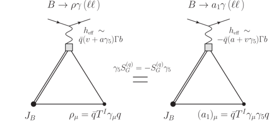
Figure 1: Diagram representing the procedure outlined in the text, using the relation (13), which necessitates both the limits $m_{q}\to 0$ and ${\left\langle\bar{q}q\right\rangle}\to 0$ in (8). The argument only requires that the weak vertex $h_{\textrm{eff}}$ be a local operator, and thus applies to both SD (form-factor) and LD (charm-loop) contributions. Note that the argument also applies to the annihilation topology where the photon is emitted from the $b$-quark or light-quark lines in the triangle graph. The schematic correlation functions on the left and right are exactly equal, from where the information on the matrix elements can be assessed via the LSZ formalism or dispersion relations, when taking into account finite-width effects. Corrections to this exact equality, beyond the chiral symmetry limit, are discussed in section 3.

In establishing our main result, the path-integral formalism, with quarks propagating in a background gluon field, will prove powerful. The $\rho$- and $a_{1}$-meson can be represented by the interpolating currents, with isospin $I$,

$$\rho_{\mu}^{I}=\bar{q}\gamma_{\mu}T^{I}q\;,\quad(a_{1})_{\mu}^{I}=\bar{q}\gamma_{\mu}\gamma_{5}T^{I}q\;,$$ (9)

while the $B$-meson $J^{PC}=0^{-+}$ can be interpolated by $J_{B}=\bar{b}\gamma_{5}q$. The correlation function

$${\cal M}^{[V]}_{(v,a)}\equiv\langle 0|TJ_{B}(x)V^{I}_{\mu}(y)h_{\textrm{eff}}(0)|0\rangle\;,$$ (10)

provides all the necessary information to understand the properties of the matrix element $\langle V|H_{\textrm{eff}}|B\rangle$, e.g. by using the LSZ formalism or dispersion representations in case finite-width effects are to be studied. Above, $V^{I}_{\mu}$ stands for either of the interpolating currents defined in (9), and

$$h_{\textrm{eff}}=\bar{q}(v+a\gamma_{5})\Gamma b\,O_{r}\;,$$ (11)

is a schematic substitute for $H_{\textrm{eff}}$ (4), where $(v,a)=(1,\pm 1)$ correspond to $O$- and $O^{\prime}$-like operators. SD and LD charm contributions correspond to $O_{r}\sim 1,\bar{c}\Gamma_{r}c$ for example. Lorentz/colour contractions over $\Gamma$ and $\Gamma_{r}$ are suppressed, as these have no impact on our argument. Integrating out the quarks in the path integral, the matrix element (10) assumes the form

$${\cal M}^{[\rho^{0}]}_{(v,a)}\sim\int D\mu_{G}{\textrm{Tr}}[(v+a\gamma_{5})S_{G}^{(b)}(0,x)\gamma_{5}S_{G}^{(d)}(x,y)\gamma_{\mu}S_{G}^{(d)}(y,0)]\;,$$ (12)

where $D\mu_{G}=DG_{\mu}\det(\not{D}+iM_{f})e^{iS(G)}$ ($D_{\mu}=(\partial-igG)_{\mu}$) is the path integral measure, $S(G)$ the Yang-Mills action, and $M_{f}$ denotes the mass matrix, which comprises of all flavours. The quark propagator in the gluon background field is $S^{(q)}_{G}(w,z)=\langle w|(\not{D}+im_{q})^{-1}|z\rangle$, and obeys

$$\gamma_{5}S^{(q)}_{G}(w,z)=-S^{(q)}_{G}(w,z)\gamma_{5}\;,$$ (13)

in the restoration limit (8). We stress that (13), upon which the argument is based, necessitates both the vanishing $\text{SU}(2)_{A}\times\text{U}(1)_{A}$-violating condensates and the limit $m_{q}\to 0$, with some more detail on related matters deferred to appendix A.

2.2.2 Relating matrix elements of parity doublers

Now comes the main step, where we replace $\gamma_{\mu}\to\gamma_{\mu}(\gamma_{5})^{2}$ and use (13) to arrive at

$${\cal M}^{[a_{1}]}_{(a,v)}=-{\cal M}^{[\rho^{0}]}_{(v,a)}\;,$$ (14)

which can also be written symbolically as $H_{\textrm{eff}}^{V\pm A}|_{\rho}\to\pm H_{\textrm{eff}}^{V\pm A}|_{a_{1}}$. This relation translates into the amplitudes (2), with $CO$- and $C^{\prime}O^{\prime}$-contributions in (4):

$$\bar{\mathcal{A}}^{\bar{B}\to\rho\gamma}_{\chi}(C,C^{\prime})=\bar{\mathcal{A}}^{\bar{B}\to a_{1}\gamma}_{\chi}(-C,C^{\prime})\;.$$ (15)

Moreover, in terms of the breakdown (7), the relations (14) and (15) lead to

χ=L±1±λ~iϵiV,L0λ~iϵi′V,Lχ=R0±λ~iϵiV,Rm^d,s+ΔRei​ϕΔRλ~iϵi′V,R.fragments fragmentsχLfragmentsplus-or-minus1fragmentsplus-or-minus~𝜆𝑖ϵ𝑖𝑉𝐿0fragments~𝜆𝑖ϵsuperscript𝑖′𝑉𝐿fragmentsχRfragments0fragmentsplus-or-minus~𝜆𝑖ϵ𝑖𝑉𝑅fragments^𝑚𝑑𝑠Δ𝑅e𝑖subscriptitalic-ϕsubscriptΔ𝑅fragments~𝜆𝑖ϵsuperscript𝑖′𝑉𝑅\begin{tabular}[]{ l | l l | l l }$\bar{\mathcal{A}}^{\bar{B}\to\rho(a_{1})\gamma}_{\chi}$&$\bar{A}_{SD,\chi}$&$\bar{A}_{LD,\chi}$&$\bar{A}^{{}^{\prime}}_{SD,\chi}$&$\bar{A}^{{}^{\prime}}_{LD,\chi}$\\[5.69046pt] \hline\cr$\chi=L$&$\pm 1$&$\pm\tilde{\lambda}_{i}{\epsilon}^{i}_{V,L}$&$0$&$\tilde{\lambda}_{i}{\epsilon}^{{}^{\prime}i}_{V,L}$\\ $\chi=R$&$\phantom{\pm}0$&$\pm\tilde{\lambda}_{i}{\epsilon}^{i}_{V,R}$&$\hat{m}_{d,s}+\Delta_{R}e^{i\phi_{\Delta_{R}}}$&$\tilde{\lambda}_{i}{\epsilon}^{{}^{\prime}i}_{V,R}$\end{tabular}\;.

¯A→¯Bρ(a1)γχ¯ASD,χ¯ALD,χ¯A′SD,χ¯A′LD,χ¯A→¯Bρ(a1)γχ¯ASD,χ¯ALD,χ¯A′SD,χ¯A′LD,χ (16)

We wish to emphasise that the procedure in this section leading to (14) works for any local operator of the form in (11), and so, in particular, applies to both the LD and SD contributions, which is reflected in the second amplitude breakdown (16). This argument establishes the main point of this work, and we now turn to the discussion of how this can be applied beyond the symmetry limit.

3 Beyond the symmetry limit

We briefly discuss the question of how to isolate the relevant phenomenology using parity doubling.

3.1 Parity doubling for phenomenologically relevant vector mesons

Table 1 indicates the main $B\to V(1^{-})$ and $J^{P}=1^{+}$ $B\to A(1^{+})$ final states, which we refer to as parity doublers in this work. Note that the charge quantum number is not of importance for practical purposes, so that $1^{++}$ and $1^{+-}$ can both be considered as effective parity doublers of the $1^{--}$ (or $1^{-+}$, cf. caption of table 1) states. The interpolating operators, denoted $O_{V}$ in the table, are

$$V_{(5)}^{(I)}=\bar{q}\gamma_{\lambda}(\gamma_{5})(T^{I})q\;,\quad T_{(5)}^{(I)}=\bar{q}\sigma_{\kappa\lambda}(\gamma_{5})(T^{I})q\;,$$ (17)

where $q=u,d$, and Lorentz indices have been suppressed on the left-hand side. Vector and axial mesons couple to these currents as

$$\langle 0|V_{(5)}|V(A)\rangle\sim\eta_{\lambda}\;,\quad\langle 0|T_{(5)}|V(A)\rangle\sim\eta_{[\lambda}p_{\kappa]}\;,$$ (18)

where square brackets denote antisymmetrisation in indices. The canonical parity doublers are listed on the horizontal lines. However, by $\text{SU}(N_{F})_{V}$ flavour symmetry, it will become clear that the measurement of a single parity doubler can reveal important information on primed Wilson coefficients $C^{\prime}_{7,8}$ (and $C^{\prime}_{9,10}$) by disentangling the LD contributions.

3.2 Sources of correction to the symmetry limit

In the real world, $\text{SU}(N_{F})_{A}\times\text{U}(1)_{A}$ is broken, e.g. by $\langle\bar{q}q\rangle_{\mu=1{\textrm{\footnotesize GeV}}}\simeq(-0.24(1)\,\mbox{GeV})^{3}$, raising the question of the corrections to (14) and the resultant breakdown (16). We find it advantageous to distinguish two sources: corrections to the $\gamma_{5}$-trick (13), and those arising from the hadronic parameters of the vector mesons.

Corrections to (14), for instance, can be understood by considering the light-cone Operator Product Expansion (OPE), with the interpolating current replaced by a $B$-meson light-cone DA e.g. [30], in place of the complete path integral (12). In this case, (13) results in both $m_{q}$- and $\langle\bar{q}q\rangle$-corrections, along with other condensates. Whereas the former are parametrically small, the latter are suppressed in effect by ${\cal O}(1)|\langle\bar{q}q\rangle/M^{3}|\simeq{\cal O}(1)(1/4)^{3}$, where $M\simeq 1\,\mbox{GeV}$ is the Borel mass scale. It remains to be seen how effective this suppression is in explicit computations. The remaining corrections to the symmetric breakdown (16) arise from differences in the hadronic parameters, namely the meson mass and the DA parameters. The latter are either (partly) known or are expressible in terms of $m_{q}$, $\langle\bar{q}q\rangle$, and higher-dimensional condensates [25]. Moreover, these can be assessed experimentally, cf. section 4.

$I^{G}$	$1^{--}$	$\frac{\Gamma_{V}}{m_{V}}$	$O_{V}$	$I^{G}$	$1^{++}$	$\frac{\Gamma_{V}}{m_{V}}$	$O_{V}$	$I^{G}$	$1^{+-}$	$\frac{\Gamma_{V}}{m_{V}}$	$O_{V}$
$1^{+}$	$\rho(\text{\small{770}})$	$19.1(1)$	$(V,T)^{I}$	$1^{-}$	$a_{1}(\text{\small{1260}})$	$35(14)$	$V^{I}_{5}$	$1^{+}$	$b_{1}(\text{\small{1235}})$	$11.5(7)$	$T^{I}_{5}$
$0^{-}$	$\omega(\text{\small{782}})$	$1.08(1)$	$V,T$	$0^{+}$	$f_{1}(\text{\small{1285}})$	$1.77(1)$	$V_{5}$	$0^{-}$	$h_{1}(\text{\small{1170}})$	$31.0(5)$	$T_{5}$
$0^{-}$	$\phi(\text{\small{1020}})$	$0.417(2)$	$(V,T)^{\bar{s}s}$	$0^{+}$	$f_{1}(\text{\small{1420}})$	$3.8(2)$	$V^{\bar{s}s}_{5}$	$0^{-}$	$h_{1}(\text{\small{1380}})$	$6.3(16)$	$T^{\bar{s}s}_{5}$
$I$	$1^{-}$				$1^{+}$				$1^{+}$
$\frac{1}{2}$	$K^{*}(\text{\small{895}})$	$5.6(1)$	$(V,T)^{s}$	$\frac{1}{2}$	$K_{1}(\text{\small{1270}})$	$7.1(16)$	$V^{s}_{5}$	$\frac{1}{2}$	$K_{1}(\text{\small{1400}})$	$12.0(9)$	$T^{s}_{5}$

Table 1: Mass ($m_{V}$) and width ($\Gamma_{V}$) data for the neutral mesons, from the latest PDG data [31]. Uncertainties in these parameters are also indicated in brackets alongside the central values. The $I^{G}$ and $J^{PC}$ quantum numbers have also been indicated. The $K$ particles are separated, as they do not have definite $G$-parity states. The two $K_{1}$-particles are subject to a mixing angle $\theta_{K_{1}}$, which is fortunately known to reasonable accuracy [32]. Mixing between particles in the same column has to be taken into account as well, cf. appendix C of [33] for the discussion of the $1^{--}$-states for example. The interpolating operators under the $O_{V}$-column are described in the main text in (17) and superscripts $s$ and $\bar{s}s$ denote replacements of the light quarks $q\to s$. In addition, there are “exotic” $1^{-+}$ states, with interpolating operators of the type $O_{V}\sim\bar{q}\gamma_{\lambda}T^{I}\overset{\leftrightarrow}{D}_{\mu}q$ and $\bar{q}\sigma_{\lambda\kappa}T^{I}\overset{\leftrightarrow}{D}_{\mu}q$. The $\pi_{1}(\text{\small{1400}})$ [31] $(I^{G}=1^{-})$ is a candidate particle for carrying these quantum numbers. Such states are rather broad, e.g. $\Gamma_{\pi_{1}}/m_{\pi_{1}}\sim 1/4$, and are not well-studied. The particle content of some non-exotic states in the table remains to be definitively established [31], but all states are expected to have significant $\bar{q}q$-wave functions. For example, from ALEPH data [34], e.g. figures 63 and 65, it can be inferred that the statement above is correct for $a_{1}(1260)$. The determination of the $3$-particle content, or the matrix element $\langle 0|\bar{q}Gq|V(A)\rangle$, is an important problem which deserves assessment from lattice QCD, in addition to the existing QCD sum rule results.

4 Applications to experimental searches

4.1 Right-handed currents from time-dependent rates

A relevant question is how to test the chirality hierarchy (7). The decay rate does not lend itself to such tests, as the right-handed amplitude is dominated by the left-handed one. The situation is, however, favourable in the case where the $B$-meson is neutral and undergoes mixing [2] (and/or decays to at least 3 hadrons and a photon [21, 35, 36, 37]). The mixing is driven by particle and antiparticle having a common final state, e.g. $\bar{B}\to V\gamma_{L}\leftarrow B$. In this case, one of the amplitudes is chirally suppressed, giving rise to a direct linear behaviour in right-handed amplitudes, $\Gamma_{\textrm{mix}}\sim\bar{\mathcal{A}}_{R}$, compared to the unfavourable behaviour of the $t=0$-rate $\Gamma\sim|\bar{\mathcal{A}}_{L}|^{2}+|\bar{\mathcal{A}}_{R}|^{2}$.

The time-dependent rate of a $B_{D}$ meson, produced at $t=0$, assuming CPT-invariance and $|q/p|=1$, takes the form

$${\cal B}(\bar{B}_{D}[B_{D}]\to V\gamma)=B_{0}e^{-\Gamma_{D}t}[{\textrm{ch}}(\frac{\Delta\Gamma_{D}}{2}t)-H{\textrm{sh}}(\frac{\Delta\Gamma_{D}}{2}t)\mp C\cos(\Delta m_{D}t)\pm S\sin(\Delta m_{D}t)]\;,$$ (19)

where $\Delta\Gamma_{D}\equiv\Gamma^{(H)}_{D}-\Gamma^{(L)}_{D}$ is the width difference, and $\Delta m_{D}\equiv m^{(H)}_{D}-m^{(L)}_{D}$ the mass difference, of the heavy ($H$) and light ($L$) mass eigenstates. The quantities $S$ and $C$ are related to indirect and direct CP violation respectively. In the Particle Data Group (PDG) notation [31], $H\equiv{\cal A}^{\Delta\Gamma}$. In terms of the decomposition (2), dropping the superscripts for brevity, these quantities read (${\cal N}=|\mathcal{A}_{L}|^{2}+|\bar{\mathcal{A}}_{L}|^{2}+|\mathcal{A}_{R}|^{2}+|\bar{\mathcal{A}}_{R}|^{2}$)

$$S(H) \;=\; 2{\textrm{Im}(\textrm{Re})}\left[\frac{q}{p}(\bar{\mathcal{A}}_{L}\mathcal{A}_{L}^{*}+\bar{\mathcal{A}}_{R}\mathcal{A}_{R}^{*})\right]{\cal N}^{-1}\;,$$ (20)

and we quote $C=\left((|\mathcal{A}_{L}|^{2}+|\mathcal{A}_{R}|^{2})-(|\bar{\mathcal{A}}_{L}|^{2}+|\bar{\mathcal{A}}_{R}|^{2})\right){\cal N}^{-1}$, although this observable is of no further relevance for this work.

In the SM, there are three weak phases orginating from $\lambda_{u,c,t}$, one of which can be eliminated by the unitarity relation $\lambda_{u}+\lambda_{c}+\lambda_{t}=0$. Hence, one may write

$$\bar{\mathcal{A}}_{L} \;\sim\; (1 \;+\; \tilde{\lambda}_{i}\,{\epsilon}^{i}_{V,L})\quad \Rightarrow \quad\mathcal{A}_{R}\sim\xi_{V}(1 \;+\; \tilde{\lambda}_{i}^{*}\,{\epsilon}^{i}_{V,L})\;,$$

$$\bar{\mathcal{A}}_{R} \;\sim\; (\hat{C_{7}^{\prime}} \;+\; \tilde{\lambda}_{i}\,{\epsilon}^{i}_{V,R})\quad \Rightarrow \quad\mathcal{A}_{L}\sim\xi_{V}(\hat{C_{7}^{\prime}} \;+\; \tilde{\lambda}_{i}^{*}\,{\epsilon}^{i}_{V,R})\;,$$ (21)

where the result on the right follows by CP conjugation, and $\xi_{V}$ is the CP eigenvalue of $V$. The observables $S$ and $H$ take the form

$$S(H)_{V(A)\gamma} \;=\; 2\xi_{V}\{ \pm (\hat{m_{D}}\!\!\begin{array}[]{c}\sin\\[-8.5359pt] \cos\end{array}\!\!(2\phi_{t}-\phi_{B_{D}})+\Delta_{R}\!\!\begin{array}[]{c}\sin\\[-8.5359pt] \cos\end{array}\!\!(2\phi_{t}+\phi_{R}-\phi_{B_{D}}))\;+$$ (26)

$$|\tilde{\lambda}_{i}|{\textrm{Re}}[{\epsilon}^{i}_{V(A),R}]\!\!\begin{array}[]{c}\sin\\[-8.5359pt] \cos\end{array}\!\!(\phi_{t}+\phi_{i}-\phi_{B_{D}})\}(1+{\cal O}(\hat{m}_{D},\Delta_{R},{\epsilon}^{i}_{V(A),\chi}))\;,$$ (29)

where the sines and cosines refer to $S$ and $H$, and the signs $\pm$ follow from the breakdown (16). Corrections to (26) can be expected to be small, and are not difficult to restore, but we have chosen to present a simple formula for illustrative purposes.

It is instructive to expand (26) for specific modes. There are four classes of $B\to V\gamma$ decays, due to the choice of initial state meson, $B_{d}$ or $B_{s}$, while the transition itself can be either $b\to d$ or $b\to s$. Since $\Delta\Gamma_{d}$ is too small to have an observable effect, this makes the $H_{B_{d}}$ parameter unobservable in practice. Below, we present the observables (26) for three of these classes, postponing details on $B_{s}\to\bar{K}^{*}$ ($b\to s$) to [13] as the decay is experimentally less attractive. The formulae in (26) take the form

$$S_{B_{d}\to\rho(a_{1})\gamma} \;\simeq\; 2\{\pm\Delta_{R}\sin\phi_{R}+\sin\beta|\tilde{\lambda}_{c}^{(d)}|\textrm{Re}[{\epsilon}^{c}_{\rho(a_{1}),R}]-\sin(\beta+\gamma)|\tilde{\lambda}_{u}^{(d)}|\textrm{Re}[{\epsilon}^{u}_{\rho(a_{1}),R}]\}\,,$$

$$S_{B_{d}\to K^{*}(K_{1})\gamma} \;\simeq\; 2\xi_{K^{*}(K_{1})}\{\mp(\Delta_{R}\sin(2\beta-\phi_{R})+\hat{m}_{s}\sin 2\beta)+\sin 2\beta\,\textrm{Re}[{\epsilon}^{c}_{K^{*}(K_{1}),R}]\}\,,$$

$$S_{B_{s}\to\phi(f_{1})\gamma} \;\simeq\; 2\{\pm\Delta_{R}\sin(\phi_{R})\}\,,$$

$$H_{B_{s}\to\phi(f_{1})\gamma} \;\simeq\; 2\{\pm(\Delta_{R}\cos(\phi_{R})+\hat{m}_{s})-\textrm{Re}[{\epsilon}^{c}_{\phi(f_{1}),R}]\}\,,$$ (30)

where $\tilde{\lambda}_{c,u}^{(d)}=O(1)$, $\tilde{\lambda}^{(s)}_{u}\ll\tilde{\lambda}^{(s)}_{c}\equiv\lambda_{c}^{(s)}/\lambda_{t}^{(s)}\simeq-1$, and we have used $\xi_{V,A}=1$. For $S_{B_{d}\to K^{*}(K_{1})\gamma}$, either (near) CP eigenstate ($K_{S,L}\pi^{0}$) can be observed in the subsequent decay, so we indicate the explicit CP eigenvalue $\xi_{K^{*}(K_{1})}$ in this case. The vanishing of $S_{B_{s}\to\phi(f_{1})\gamma}\simeq 0$ in the SM comes from the cancellation of all weak phases involved, and this quantity is therefore a null test for weak phases of RHC.

The expressions (4.1) are for the $J^{PC}=1^{++}$ parity doublers. If, instead, one were to use doublers with the $J^{PC}=1^{+-}$ quantum numbers, then $\xi_{(1^{+-})}=-1$, and the corresponding observables $S$ and $H$ pick up an additional minus sign.

4.2 The approach exemplified in $B_{s}\to\phi(f_{1})\gamma$

From (4.1), it can be seen that both observables $S$ and $H$ in (26) are of interest, and can be observed experimentally, in the decay $B_{s}\to\phi(f_{1}/h_{1})\gamma$, where $f_{1}\equiv f_{1}(\text{\small{1420}})$ and $h_{1}\equiv h_{1}(\text{\small{1380}})$. Using $\xi_{h_{1}}=-1$, one gets a remarkable equation

$$\left(H_{\phi\gamma}\pm H_{f_{1}(h_{1})\gamma}\right) \;\simeq\; -2{\textrm{Re}}[{\epsilon}^{c}_{\phi,R}+{\epsilon}^{c}_{f_{1}(h_{1}),R}]$$

$$\;=\; -2{\textrm{Re}}[{\epsilon}^{c}_{\phi,R}](1+\mathbb{R}_{f_{1}(h_{1}),\phi}^{c})\;,$$ (31)

where

$$\mathbb{R}_{A,V}^{i}\equiv\frac{\textrm{Re}[{\epsilon}^{i}_{A,R}]}{\textrm{Re}[{\epsilon}^{i}_{V,R}]}=1+{\cal O}(m_{q},\langle\bar{q}q\rangle)\;.$$ (32)

and the $\simeq$ in (4.2) indicates the approximations made in (26), as well as neglecting the $\lambda_{u}$ LD contribution. Eq. (4.2) is remarkable in that it shows that it is possible to measure the sum of the LD (charm) contributions without any compromise from the symmetry breaking, thanks to the exact form factor relation $T_{1}(0)=T_{2}(0)$. In extracting the LD contribution, what matters is not how far away $\mathbb{R}_{A,V}$ is from unity but the uncertainty itself. As an example, supposing we could determine $\mathbb{R}_{A,V}$ to $20\%$ uncertainty, with $\mathbb{R}_{A,V}$ being one of the four values $(1,1.2,1.5,2)$. Then one could extract ${\epsilon}^{c}_{\phi,R}$ from experiment with an accuracy of $(10,11,12,13)\%$ respectively. This is very much improved situation in two ways. Firstly, one can extract the LD contribution by solely predicting the uncertainty on $\mathbb{R}_{A,V}^{i}$ rather than the LD matrix element itself. In addition, this translates into a considerably smaller uncertainty of the LD matrix element than one could hope to get from an a priori computation.

Finally, we mention that the counterpart of (4.2) is the equation where the SD part is enhanced and the LD part reduced, and reads

$$\Delta_{R}\cos(\phi_{\Delta_{R}})=\frac{1}{4}(H_{\phi\gamma}\mp H_{f_{1}(h_{1})\gamma})+\frac{1}{2}\textrm{Re}[{\epsilon}^{c}_{\phi,R}-{\epsilon}^{c}_{f_{1}(h_{1}),R}]-\hat{m}_{s}\;.$$ (33)

It remains to be seen in the future how well such quantities can be measured and how well the ratios $\mathbb{R}_{A,V}^{i}$ can be predicted. It is clear that the potential improvement is significantly larger than what can be hoped for in a direct computation, as many uncertainties will cancel, some of them due to the symmetry limit.

4.3 $B\to V\ell\bar{\ell}$ and other decay channels

Decays such as $B\to K^{*}(\to K\pi)\mu^{+}\mu^{-}$ are an important probe of NP in the flavour sector [39, 40, 41, 42], as their angular distributions allow the assessment of a wealth of observables, twelve for the dimension-six $H_{\textrm{eff}}$ [43]; higher-dimensional operators are also accessible by extracting higher moments (modulo QED effects) [28].

The parity-doubling approach can be extended to $B\to(V,A)\ell\bar{\ell}$ rather straightforwardly by considering the angular observables. In the notation of [28], the moments, or angular coefficients, are $\mathbb{G}_{m}^{l_{k},l_{\ell}}$, where $l_{k,\ell}$ denote the partial wave of the $K\pi$ and $\mu\mu$-pair respectively, and $m$ is the relative helicity difference. An interference of left- and right-handed polarisation corresponds to the helicity difference $m=2$, which leads to the real and imaginary parts of $\mathbb{G}_{m}^{l_{K},l_{\ell}}\to\mathbb{G}_{2}^{2,2}$ being the observables of interest. These have indeed been identified, with the acronyms $P_{1}=A_{T}^{(2)}\sim\textrm{Re}[\mathbb{G}_{2}^{2,2}]$, $P_{3}\sim\textrm{Im}[\mathbb{G}_{2}^{2,2}]$, some time ago (e.g. [44, 45]) as giving access to RHC at low $q^{2}$. A measurement of the right-handed LD contribution at $q^{2}=0$, or at low $q^{2}$, could also provide invaluable information on the angular anomalies [46] (most notably, $P_{5}^{\prime}\sim\textrm{Re}[\mathbb{G}_{1}^{2,1}]$) observed in $B\to K^{*}\ell\bar{\ell}$ at LHCb, in connection with approaches using analyticity [47, 48]. In this respect, $B\to K^{*}e^{+}e^{-}$ is an even more promising channel, studied at the LHCb experiment [49], and with good prospects at Belle II. Exploring the potential of time-dependent angular distributions would also seem to be an interesting possibility [50].

Thus, $B\to(V,A)\ell\bar{\ell}$ allows the assessment of all the right-handed operators $O^{\prime}_{7,8,9,10}$, or their respective Wilson coefficients, without resorting to time-dependent amplitudes, meaning that decay modes for charged mesons can also be assessed in this manner.

We wish to emphasise that the ideas in this paper, whilst they have been discussed primarily in the context of $B\to(V,A)\gamma$ and $B\to(V,A)\ell\bar{\ell}$ decays, can be extended to other decays of interest, as long as such systems admit parity-doubling partner decays. Examples include the $D\to V\gamma(\ell\bar{\ell})$ sector, e.g. [51, 52], as well as higher-spin states e.g. $B\to K_{2}\gamma(\ell\bar{\ell})$, since parity doubling occurs in those modes [20]. Applications to symmetry-based amplitude parametrisations in $B\to PV(A)$, with $P$ being a pseudoscalar meson, are another possibility, although one would expect stronger breaking effects in final-state interactions than in the LD amplitude of radiative decays.

5 Discussion and conclusions

In this paper, we have advocated that the contamination of right-handed currents in $B\to V\gamma(\ell\bar{\ell})$ decays due to long-distance effects can be controlled by considering in addition the corresponding decay $B\to A\gamma(\ell\bar{\ell})$. It was shown, in the chiral symmetry restoration limit (8), that the leaking of the V-A contributions into the right-handed amplitude for the parity doublers comes with exactly the opposite sign, as compared to the leading short-distance contributions (16).

The case beyond the symmetry limit is briefly discussed in the previous section for $B\to V(A)\ell\bar{\ell}$, and for $B\to V(A)\gamma$ the summary is as follows. The sum of the vector and axial long-distance contribution can still be extracted from experiment (e.g. (4.2)), because of the exact form factor relation $T_{1}(0)=T_{2}(0)$. This then allows to test theory predictions of exclusive long-distance contributions [16, 14, 54, 13] and contrast them with the, somewhat larger, indirect estimation from the inclusive $b\to X_{s}\gamma$ channel [12]. More concretely, the charm contamination was computed to be $0.6\%$ for $S_{B_{d}\to K^{*}\gamma}$ in [16], whereas [12] estimated the contaminations to be up to $6\%$. In addition, the smallness of the theoretical result can be understood by invoking the parity-doubling limit [13].

From (4.2) one can extract the sum of the axial and vector long-distance contribution. One can obtain the individual contributions by taking into account a theory prediction of the ratio $\mathbb{R}_{A,V}$ (32), which comes with reduced uncertainty due to standard uncertainty cancellations, further enhanced by the symmetry limit. An error on $\mathbb{R}_{A,V}$ of $20\%$ results in an uncertainty on the single long-distance contribution of just around $10\%$, if no experimental error is assumed. In summary, we have proposed a data-theory-driven program to reduce the uncertainty of the long-distance contamination, paving the way to much cleaner searches for right-handed currents.

Let us turn at last to the experimental perspectives. For Belle II, an uncertainty of $3\%$ is anticipated in this observable with a data set of $50\,\textrm{ab}^{-1}$ [55]. This estimate does not yet take into account the gain in photon efficiency in differences and sums of rates, relevant to the parity-doubling approach cf. (4.2,33). The analysis of axial vector meson final states is more challenging, because of their decay chains. However, the measurement of a single channel can still provide invaluable information on the long-distance contributions (4.2), as they are related by $\text{SU}(N_{F})_{V}$ flavour symmetry, taking into account normalisation issues such as mixing angles. Promising states are the $K_{1}(1270)$ and the $f_{1}(\text{\small{1285}})$ or $f_{1}(\text{\small{1420}})$. Belle has reported a time-dependent measurement of $B^{0}\to\rho^{0}K_{s}\gamma$ [56] and the rate ${\cal B}(B^{+}\to K^{+}_{1}(1270)\gamma)\simeq 4.3(9)(9)\cdot 10^{-5}$ [57]. At the LHCb experiment, the $K_{1}$ states were seen in $B\to K^{+}\pi^{+}\pi^{-}$ at the LHCb [58], and the first observation of ${\cal B}\left(B_{s,d}\to f_{1}(\text{\small{1285}})J/\Psi\right)\simeq 7\cdot 10^{-5},\,8\cdot 10^{-6}$ was reported in [59].

Acknowledgements

JG and RZ are grateful to Gino Isidori for an extended and refreshing stay at the Pauli-Centre for Theoretical Physics at the University of Zürich, where a large fraction of this work has been undertaken. RZ would like to thank Johannes Albrecht, Greig Cowan, Akimasa Ishikawa, Franz Muheim, Christopher Smith, and Philip Urquijo, as well as many of the participants of QCD-Moriond-2018 and the $b\to s\ell\ell$ workshop at Miapp (TU Munich), for useful discussions. JG acknowledges the support of an STFC studentship (grant reference ST/K501980/1).

Appendix A Chiral restoration limit and $\gamma_{5}S_{G}^{(q)}=-S_{G}^{(q)}\gamma_{5}$ (13)

The pion decay constant, $F_{\pi}\simeq 92\,\mbox{MeV}$ in QCD, is defined by $\langle\pi^{b}(p)|J^{A,a}_{\mu}|0\rangle=\delta^{ab}p_{\mu}F_{\pi}$, with $J^{A,a}_{\mu}=\bar{q}T^{a}\gamma_{\mu}\gamma_{5}q$, and $q$ are $N_{F}$ light quarks. $F_{\pi}$ is the order parameter of spontaneous chiral symmetry breaking. At the heuristic level, $F_{\pi}\neq 0$ implies the non-invariance of the vacuum with respect to the axial flavour charge $Q^{A,a}=\int_{V}d^{3}xJ^{A,a}_{0}$. In this appendix, we aim to show that our formula (13),

$$m_{q},\langle\bar{q}q\rangle=\dots=0\quad\Leftrightarrow\quad\gamma_{5}S_{G}^{(q)}(w,z)=-S_{G}^{(q)}(w,z)\gamma_{5}\quad\left(\Leftrightarrow\quad F_{\pi}=0\right)\,,$$ (34)

depends, as expected, on the restoration limit. This result serves to illustrate (13) in some more detail than discussed in the main text.

We first proceed to show that $\gamma_{5}S_{G}^{(q)}(w,z)=-S_{G}^{(q)}(w,z)\gamma_{5}\quad\Rightarrow\quad F_{\pi}=0$. For this purpose, consider the correlation function, used to derive the Weinberg sum rules [18],

$$(\Pi^{a,b}_{LR})_{\mu\nu}(q^{2})=i\int d^{4}xe^{iq\cdot x}\langle TJ^{a,L}_{\mu}(x)J^{b,R}_{\nu}(x)\rangle=(q_{\mu}q_{\nu}-q^{2}g_{\mu\nu})\Pi^{a,b}_{LR}(q^{2})\;,$$ (35)

where $J^{a,L(R)}_{\mu}=2\bar{q}T^{a}\gamma_{\mu}(\gamma_{5})q_{L(R)}$, and $(a,b)$ are $\text{SU}(N_{F})_{(L,R)}$ flavour indices. One may integrate out the fermion in the path integral formulation to obtain

$$(\hat{\Pi}^{a,b}_{\textrm{LR}})_{\mu\nu}(x)=\frac{1}{2}\delta^{ab}\int D\mu_{G}\left(\textrm{Tr}[S_{G}^{(q)}(x,0)\gamma_{\mu}S^{(q)}_{G}(0,x)\gamma_{\nu}]-\textrm{Tr}[S^{(q)}_{G}(x,0)\gamma_{\mu}\gamma_{5}S^{(q)}_{G}(0,x)\gamma_{\nu}\gamma_{5}]\right)\;,$$ (36)

where the hat denotes the Fourier transform, and the path integral measure, already defined below Eq. (12), is $D\mu_{G}=DG_{\mu}\det(\not{D}+iM_{f})e^{iS(G)}$. Using $\gamma_{5}S_{G}^{(q)}(w,z)=-S_{G}^{(q)}(w,z)\gamma_{5}$ (13), one concludes that $(\hat{\Pi}^{a,b}_{\textrm{LR}})_{\mu\nu}(x)=0$ by commuting the $\gamma_{5}$ through the fermion propagator and the $\gamma$-matrix in (36). Since $4(\Pi^{a,b}_{LR})_{\mu\nu}=\delta^{ab}((\Pi_{VV})_{\mu\nu}-(\Pi_{AA})_{\mu\nu})$, the spectral densities

$$\rho_{V}(s)=\rho_{A}(s)\;,$$ (37)

of the dispersion representation ($\pi\rho_{V,A}(s)=\textrm{Im}[\Pi_{VV(AA)}(s)]$)

$$\Pi_{V(A)}(q^{2})=\int_{0}^{\infty}ds\frac{\rho_{V(A)}(s)}{s-q^{2}-i0}\;,$$ (38)

are point-by-point identical. The spectral densities are given by

$$\rho_{A}(s)=F_{\pi}^{2}\delta(s-m_{\pi}^{2})+F_{a_{1}}^{2}\delta(s-m_{a_{1}}^{2})+\dots\;,\quad\rho_{V}(s)=F_{\rho}^{2}\delta(s-m_{\rho}^{2})+\dots\;,$$ (39)

where the dots stand for higher states, and the fact that we used the narrow width approximation for the $\rho$ and $a_{1}$ meson is immaterial. The only crucial point is that (37) necessarily implies $F_{\pi}=0$, since there is no massless particle in the vector channel.

In the second part, we show that $m_{q},\langle\bar{q}q\rangle={\left\langle\bar{q}\sigma\!\cdot\!Gq\right\rangle}=\dots=0\quad\Leftrightarrow\gamma_{5}S_{G}^{(q)}(w,z)=-S_{G}^{(q)}(w,z)\gamma_{5}$, which is what was used in the main text in section 2.2.1. In practical computations, using the OPE one uses the formula [60]

$$\langle\bar{q}_{m}(x_{1})q_{n}(x_{2})\rangle=N_{c} \left[\frac{1}{12}\left(1+\frac{i}{d}m_{q}\not{x}_{12}\right)_{nm}{\left\langle\bar{q}q\right\rangle}+\frac{g^{2}}{288}\left(\frac{i}{12}x_{12}^{2}(\not{x}_{12})_{nm}\langle V^{a}_{q}V^{a}_{f}\rangle\right)\right.$$

$$\left.+\frac{1}{192}x_{12}^{2}(1+\frac{i}{6}m_{q}\not{x}_{12})_{nm}{\left\langle\bar{q}\sigma\!\cdot\!Gq\right\rangle}+\dots\right]$$ (40)

where $x_{12}\equiv(x_{1}-x_{2})$, $m$ and $n$ are Dirac indices, $\langle V^{a}_{q}V^{a}_{f}\rangle=\langle\bar{q}\gamma_{\mu}t^{a}q\sum_{f}\bar{f}\gamma^{\mu}t^{a}f\rangle$, and the dots stand for higher dimensional condensates. We only consider the terms which do not vanish in the $m_{q}\to 0$ limit. It is readily seen that ${\left\langle\bar{q}q\right\rangle}$ and ${\left\langle\bar{q}\sigma\!\cdot\!Gq\right\rangle}$ are obstructions to (13), which is expected since they are not invariant under $\text{SU}(N_{F})_{A}$ (and $\text{U}(1)_{A}$). The contrary applies to $\langle V^{a}_{q}V^{a}_{f}\rangle$. The statement about $\langle\bar{q}q\rangle$ can be made slightly more rigorous. Following the argument of [61], the fermion propagator in the external gluon field may be written as

$$\langle q(x)\bar{q}(0)\rangle_{G}=iS_{G}(x,0)=\sum_{n}\frac{\phi_{n}(x)\phi_{n}^{\dagger}(0)}{m_{q}-i\lambda_{n}}$$ (41)

where $\phi_{n}$ are the Dirac operator eigenmodes $i\not{D}\phi_{n}=\lambda_{n}\phi_{n}$. Noting that $\gamma_{5}\phi_{n}$ is an eigenmode of eigenvalue $-\lambda_{n}$, and that the zero eigenmodes are suppressed by $V^{-1/2}$ in the infinite-volume limit, one finds

$$\langle\bar{q}q\rangle=\frac{1}{V}\int_{V}d^{4}x\langle\bar{q}q\rangle\stackrel{{\scriptstyle V\to\infty}}{{\to}}-2m_{q}\int_{0}^{\infty}d\lambda\frac{\rho(\lambda)}{m_{q}^{2}+\lambda^{2}}\;,$$ (42)

where the function $\rho(\lambda)$ is the Dirac eigenmode density. In the limit $m_{q}\to 0$, one obtains the celebrated Banks-Casher relation $\langle\bar{q}q\rangle=-\textrm{sign}(m)\,\pi\rho(0)$ [61]. Therefore, one concludes that $\langle\bar{q}q\rangle=0$ ($\rho(0)=0$) is a necessary condition for $\gamma_{5}S^{(q)}_{G}(w,z)=-S^{(q)}_{G}(w,z)\gamma_{5}$ (13) to hold. Similar arguments would apply to further terms in (A), but are more difficult to render rigorous. Since $F_{\pi}=0\Rightarrow m_{q},\langle\bar{q}q\rangle=\dots=0$, this finally results in (34).

Appendix B Parity doubling

In this section, we provide some minimal background on parity doubling, which has a long history in particle physics [20]. Parity doubling achieved its modern paradigm shift with the advent of the Weinberg sum rules [18], partly described in the previous section, and has recently been investigated on the lattice [62, 63, 64].^,

The basic idea is that a global symmetry, generated by a charge $Q$, induces degeneracies in the spectrum, as it commutes with the Hamiltonian. Examples include supersymmetry, with degeneracies between bosons and fermions, or simply the global $\text{SU}(N_{f})_{V}$ flavour symmetry, leading to isospin multiplets. In the restoration limit (8), which leads to the enhanced flavour symmetry $\text{SU}(N_{f})_{V}\to\text{SU}(N_{f})_{V}\times\text{SU}(N_{f})_{A}\times\text{U}(1)_{A}$, the same types of degeneracy can be expected. There is, however, another important point that accompanies this effect: namely, that the additional global symmetry gives rise to new quantum numbers.

For the sake of concreteness, let us choose $N_{f}=2$ below. In the case at hand, $\text{SU}(2)_{V}\times\text{SU}(2)_{A}\simeq\text{SU}(2)_{L}\times\text{SU}(2)_{R}$, this leads to both a left- and right-handed isospin quantum number $(I_{L},I_{R})$ instead of just the isospin $I_{V}$ itself. The classification of the representations is discussed in [69]. More precisely, the particles are classified according to the parity-chiral group $\text{SU}(2)\times\text{SU}(2)\times C_{i}$, where $C_{i}$ is the space reflection. The lowest irreducible representations $(I_{L},I_{R})$, of dimension $(2I_{L}+1)(2I_{R}+1)$, are listed in figure 2. The splitting from left to right can be understood as the branching rule of $(I_{L},I_{R})|_{\text{SU}_{V}(2)}$; e.g. $(1/2,1/2)_{a}|_{\text{SU}_{V}(2)}\to 3_{b_{1}^{\perp}}+1_{\omega^{\perp}}$. The two interpolating currents discussed as templates in the text (17) correspond to the $(1,0)\oplus(0,1)$ multiplet. The two $(1/2,1/2)$ representations denoted by superscripts $a$ and $b$ are distinct by the parity operation. The use of $\parallel$ and $\perp$ as superscripts is non-standard, and inspired by the notation of the corresponding decay constants. As a last generic remark, let us add that, in the real world, the $\rho$ and the $\rho^{\prime}=\rho(\text{\small{1450}})$ are admixtures of the $\rho^{\parallel}$ and $\rho^{\perp}$-states. In the following subsection, we give an example where one can explicitly see how the $\text{U}(1)_{A}\times\text{SU}(2)_{A}$-violating condensates control differences in the hadronic data between the $\rho$ and $a_{1}$.

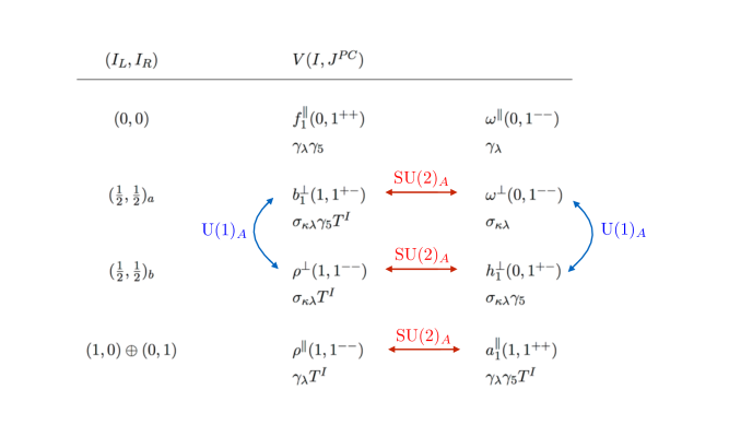
Figure 2: Lowest-lying particles coupling to vector and tensor currents of isosinglet- and isotriplet-type, making a total of $16$ vector mesons. For simple comparison, we use the same graphic presentation with similar notation as used in [62]. The interpolating operators are defined in (17) where the coupling to the states is specified further below. In the restoration limit (8), one would expect a $4$-, $4$- and $6$-plet degeneracy by the restoration of the $\text{SU}(2)_{A}$ (red arrows). In the case where $\text{U}(1)_{A}$ (blue arrows) symmetry is also restored, this leads to a $8$- and $6$-plet degeneracy. The actual degeneracy is found to be larger [62], compatible with an emergent $\text{SU}(4)$ [70] (or even $\text{SU}(4)\times\text{SU}(4)$ [71]) symmetry.

B.1 The Weinberg sum rules as an example

From group-theoretic considerations, one can argue that the first correction to the chirality correlation function (35) is given by $(\Pi^{a,b}_{LR})_{\mu\nu}(q^{2})\sim\langle O_{\chi SB}\rangle Q^{-6}+O(Q^{-8})$, where $q^{2}\equiv-Q^{2}$ (e.g. [72]), $4O_{\chi SB}=\bar{q}T^{3}\lambda^{i}q_{L}\bar{q}T^{3}\lambda^{i}q_{R}$, and $\lambda^{i}$ are the $\text{SU}(3)$ colour matrices. One can then power-expand the denominator and arrive at the first two Weinberg sum rules

$$\int_{0}^{\infty}s^{n}(\rho_{V}(s)-\rho_{A}(s))=0\;,\quad n=0,1\;.$$ (43)

The leading correction, or the third sum rule, is given by

$$\int_{0}^{\infty}s^{2}(\rho_{V}(s)-\rho_{A}(s))=2\pi\alpha_{s}\langle O_{\chi SB}\rangle\;.$$ (44)

So far, everything is exact. Since the correlation functions are well-described at high $q^{2}$ by perturbation theory, which is equal for the $V$- and the $A$-channel, $\rho_{V}(s)\simeq\rho_{A}(s)$ will hold for some $s>s_{0}$. Weinberg [18] assumed that $s_{0}$ is just above the $a_{1}$ resonance, and restricted himself to the parametrisations found in (39), from which he deduced

$$F_{\rho}^{2}-F_{\pi}^{2}-F_{a_{1}}^{2} \;=\; 0\;,$$

$$m_{\rho}^{2}F_{\rho}^{2}-m_{a_{1}}^{2}F_{a_{1}}^{2} \;=\; 0\;,$$

$$m_{\rho}^{4}F_{\rho}^{2}-m_{a_{1}}^{4}F_{a_{1}}^{2} \;=\; 2\pi\alpha_{s}\langle O_{\chi SB}\rangle\;.$$ (45)

These sum rules are rather well-satisfied at the empirical level. The last equation nicely illustrates, in a concrete setting, how the restoration limit is controlled by the $\text{SU}(2)_{A}\times\text{U}(1)_{A}$-violating condensate $\langle O_{\chi SB}\rangle$. We note that, in the vacuum factorisation approximation, $\langle O_{\chi SB}\rangle=-\frac{N_{c}^{2}-1}{N_{c}^{2}}\langle\bar{q}q\rangle^{2}$ [60].

Appendix C Definition of effective Hamiltonian

Here we describe in more detail the effective Hamiltonian for $b\to(d,s)\gamma$ and $b\to(d,s)\ell\bar{\ell}$ decays, clarifying the notation in (4). In the basis of [73], the operators contributing to (4) are: the four-quark tree-level operators

$$O^{U}_{1} ={\bar{D}}_{L,i}\gamma_{\mu}U_{j}\bar{U}_{L,j}\gamma^{\mu}b_{i}\,,$$

$$O^{U}_{2} ={\bar{D}}_{L}\gamma_{\mu}U\bar{U}_{L}\gamma^{\mu}b\,;$$ (46)

the loop-induced four-quark operators, $O_{3,...,6}$:

$$O_{3}=\left(\bar{D}_{L}\gamma_{\mu}b\right)\sum_{q}\left(\bar{q}_{L}\gamma^{\mu}q\right)\,, \qquad\qquad O_{4}=\left(\bar{D}_{L,i}\gamma_{\mu}b_{j}\right)\sum_{q}\left(\bar{q}_{L,j}\gamma^{\mu}q_{i}\right)\,,$$

$$O_{5}=\left(\bar{D}_{L}\gamma_{\mu}b\right)\sum_{q}\left(\bar{q}_{R}\gamma^{\mu}q\right)\,, \qquad\qquad O_{6}=\left(\bar{D}_{L,i}\gamma_{\mu}b_{j}\right)\sum_{q}\left(\bar{q}_{R,j}\gamma^{\mu}q_{i}\right)\,;$$ (47)

and the electromagnetic and QCD dipoles (with $D_{\mu}=\partial_{\mu}-ig_{s}G_{\mu}-ieA_{\mu}$ convention)

$$O_{7(8)}=-\frac{e(g)}{16\pi^{2}}m_{b}{\bar{s}}_{L}\sigma\cdot F(G)b\,.$$ (48)

The $C_{i}$ are scale-dependent Wilson coefficients, which can be calculated perturbatively using renormalisation group methods (e.g. [73, 74]). The most relevant $C_{i}$ for the discussion in the paper are $(C_{2},C_{1},C_{7})(m_{b})\simeq(1,-0.13,-0.37)$.

For $b\to(d,s)\ell\bar{\ell}$ decays, one also needs the operators

$$O_{9,(10)}=\frac{\alpha_{\textrm{EM}}}{4\pi}{\bar{D}}_{L}\gamma_{\mu}b\bar{\ell}\gamma^{\mu}\left(\gamma_{5}\right)\ell\,.$$ (49)

Parity-flipped versions of the operators above can be obtained by the replacement $O^{\prime}=\left.O\right|_{{\bar{D}}_{L}\to{\bar{D}}_{R}}$, as well as (in the SM) $m_{b}\to m_{D}$ in $O_{7,8}$. The relative importance of the $O_{1,2}^{U=u,c}$ operators is dependent on the CKM hierarchy $\lambda_{U}^{(D)}=V_{Ub}^{\vphantom{*}}V_{UD}^{*}$ for $b\to d$ and $b\to s$

$$\lambda^{(s)}_{u}:\lambda^{(s)}_{c}:\lambda^{(s)}_{t}=\lambda^{4}:\lambda^{2}:\lambda^{2}\;,\qquad\lambda^{(d)}_{u}:\lambda^{(d)}_{c}:\lambda^{(d)}_{t}=\lambda^{3}:\lambda^{3}:\lambda^{3}\;,$$ (50)

respectively. Above, $\lambda$ is the Wolfenstein parameter, with the approximate value $\lambda\simeq 0.225$ [31].

References

- [1] J. G. Korner and G. R. Goldstein, “Quark and Particle Helicities in Hadronic Charmed Particle Decays,” Phys. Lett. 89B (1979) 105–110.
- [2] D. Atwood, M. Gronau, and A. Soni, “Mixing induced CP asymmetries in radiative decays in and beyond the standard model,” Phys. Rev. Lett. 79 (1997) 185–188, arXiv:hep-ph/9704272 [hep-ph].
- [3] M. Beneke, J. Rohrer, and D. Yang, “Enhanced electroweak penguin amplitude in decays,” Phys. Rev. Lett. 96 (2006) 141801, arXiv:hep-ph/0512258 [hep-ph].
- [4] K. Agashe and C. D. Carone, “Supersymmetric flavor models and the anomaly,” Phys. Rev. D68 (2003) 035017, arXiv:hep-ph/0304229 [hep-ph].
- [5] E. Lunghi and J. Matias, “Huge right-handed current effects in in supersymmetry,” JHEP 04 (2007) 058, arXiv:hep-ph/0612166 [hep-ph].
- [6] E. Kou, C.-D. Lü, and F.-S. Yu, “Photon Polarization in the processes in the Left-Right Symmetric Model,” JHEP 12 (2013) 102, arXiv:1305.3173 [hep-ph].
- [7] M. König, M. Neubert, and D. M. Straub, “Dipole operator constraints on composite Higgs models,” Eur. Phys. J. C74 no. 7, (2014) 2945, arXiv:1403.2756 [hep-ph].
- [8] S. Descotes-Genon, L. Hofer, J. Matias, and J. Virto, “Global analysis of anomalies,” JHEP 06 (2016) 092, arXiv:1510.04239 [hep-ph].
- [9] A. Paul and D. M. Straub, “Constraints on new physics from radiative decays,” JHEP 04 (2017) 027, arXiv:1608.02556 [hep-ph].
- [10] T. Hurth, F. Mahmoudi, D. Martinez Santos, and S. Neshatpour, “Lepton nonuniversality in exclusive decays,” Phys. Rev. D96 no. 9, (2017) 095034, arXiv:1705.06274 [hep-ph].
- [11] G. D’Ambrosio, G. F. Giudice, G. Isidori, and A. Strumia, “Minimal flavor violation: An Effective field theory approach,” Nucl. Phys. B645 (2002) 155–187, arXiv:hep-ph/0207036 [hep-ph].
- [12] B. Grinstein, Y. Grossman, Z. Ligeti, and D. Pirjol, “The Photon polarization in in the standard model,” Phys. Rev. D71 (2005) 011504, arXiv:hep-ph/0412019 [hep-ph].
- [13] J. Gratrex and R. Zwicky, “Long-distance charm loops in decays from light-cone sum rules.” In preparation.
- [14] F. Muheim, Y. Xie, and R. Zwicky, “Exploiting the width difference in ,” Phys.Lett. B664 (2008) 174–179, arXiv:0802.0876 [hep-ph].
- [15] P. Ball, G. W. Jones, and R. Zwicky, “ beyond QCD factorisation,” Phys.Rev. D75 (2007) 054004, arXiv:hep-ph/0612081 [hep-ph].
- [16] P. Ball and R. Zwicky, “Time-dependent Asymmetry in as a (Quasi) Null Test of the Standard Model,” Phys. Lett. B642 (2006) 478–486, arXiv:hep-ph/0609037 [hep-ph].
- [17] A. Khodjamirian, G. Stoll, and D. Wyler, “Calculation of long distance effects in exclusive weak radiative decays of meson,” Phys. Lett. B358 (1995) 129–138, arXiv:hep-ph/9506242 [hep-ph].
- [18] S. Weinberg, “Precise relations between the spectra of vector and axial vector mesons,” Phys. Rev. Lett. 18 (1967) 507–509.
- [19] S. Weinberg, The quantum theory of fields. Vol. 2: Modern applications. Cambridge University Press, 2013.
- [20] S. S. Afonin, “Parity Doubling in Particle Physics,” Int. J. Mod. Phys. A22 (2007) 4537–4586, arXiv:0704.1639 [hep-ph].
- [21] M. Gronau, Y. Grossman, D. Pirjol, and A. Ryd, “Measuring the photon polarization in ,” Phys. Rev. Lett. 88 (2002) 051802, arXiv:hep-ph/0107254 [hep-ph].
- [22] BaBar Collaboration, P. del Amo Sanchez et al., “Time-dependent analysis of decays and studies of the system in decays,” Phys. Rev. D93 no. 5, (2016) 052013, arXiv:1512.03579 [hep-ex].
- [23] E. Kou, A. Le Yaouanc, and A. Tayduganov, “Angular analysis of : towards a model independent determination of the photon polarization with ,” Phys. Lett. B763 (2016) 66–71, arXiv:1604.07708 [hep-ph].
- [24] K.-C. Yang, “Light-cone distribution amplitudes of axial-vector mesons,” Nucl. Phys. B776 (2007) 187–257, arXiv:0705.0692 [hep-ph].
- [25] J. Gratrex and R. Zwicky, “Axial and vector meson distribution amplitudes and their symmetries.” In preparation.
- [26] J. Gratrex and R. Zwicky, “Right-handed Currents Searches and Parity Doubling,” in 53rd Rencontres de Moriond on QCD and High Energy Interactions (Moriond QCD 2018) La Thuile, Italy, March 17-24. 2018. arXiv:1807.01643 [hep-ph].
- [27] G. Hiller and R. Zwicky, “(A)symmetries of weak decays at and near the kinematic endpoint,” JHEP 1403 (2014) 042, arXiv:1312.1923 [hep-ph].
- [28] J. Gratrex, M. Hopfer, and R. Zwicky, “Generalised helicity formalism, higher moments and the angular distributions,” Phys. Rev. D93 no. 5, (2016) 054008, arXiv:1506.03970 [hep-ph].
- [29] M. Dimou, J. Lyon, and R. Zwicky, “Exclusive Chromomagnetism in heavy-to-light FCNCs,” Phys.Rev. D87 no. 7, (2013) 074008, arXiv:1212.2242 [hep-ph].
- [30] A. Khodjamirian, T. Mannel, and N. Offen, “-meson distribution amplitude from the form-factor,” Phys. Lett. B620 (2005) 52–60, arXiv:hep-ph/0504091 [hep-ph].
- [31] Particle Data Group Collaboration, C. Patrignani et al., “Review of Particle Physics,” Chin. Phys. C40 no. 10, (2016) 100001.
- [32] H.-Y. Cheng, “Revisiting Axial-Vector Meson Mixing,” Phys. Lett. B707 (2012) 116–120, arXiv:1110.2249 [hep-ph].
- [33] A. Bharucha, D. M. Straub, and R. Zwicky, “ in the Standard Model from Light-Cone Sum Rules,” JHEP 08 (2016) 098, arXiv:1503.05534 [hep-ph].
- [34] ALEPH Collaboration, S. Schael et al., “Branching ratios and spectral functions of tau decays: Final ALEPH measurements and physics implications,” Phys. Rept. 421 (2005) 191–284, arXiv:hep-ex/0506072 [hep-ex].
- [35] D. Atwood, T. Gershon, M. Hazumi, and A. Soni, “Mixing-induced CP violation in in search of clean new physics signals,” Phys. Rev. D71 (2005) 076003, arXiv:hep-ph/0410036 [hep-ph].
- [36] D. Bečirević, E. Kou, A. Le Yaouanc, and A. Tayduganov, “Future prospects for the determination of the Wilson coefficient ,” JHEP 08 (2012) 090, arXiv:1206.1502 [hep-ph].
- [37] M. Gronau and D. Pirjol, “Reexamining the photon polarization in ,” Phys. Rev. D96 no. 1, (2017) 013002, arXiv:1704.05280 [hep-ph].
- [38] HFLAV Collaboration, Y. Amhis et al., “Averages of -hadron, -hadron, and -lepton properties as of Summer 2016,” Eur. Phys. J. C77 no. 12, (2017) 895, arXiv:1612.07233 [hep-ex].
- [39] LHCb Collaboration, R. Aaij et al., “Angular analysis of the decay using 3 fb-1 of integrated luminosity,” JHEP 02 (2016) 104, arXiv:1512.04442 [hep-ex].
- [40] Belle Collaboration, S. Wehle et al., “Lepton-Flavor-Dependent Angular Analysis of ,” Phys. Rev. Lett. 118 no. 11, (2017) 111801, arXiv:1612.05014 [hep-ex].
- [41] CMS Collaboration, A. M. Sirunyan et al., “Measurement of angular parameters from the decay in proton-proton collisions at 8 TeV,” Phys. Lett. B781 (2018) 517–541, arXiv:1710.02846 [hep-ex].
- [42] ATLAS Collaboration, M. Aaboud et al., “Angular analysis of decays in collisions at TeV with the ATLAS detector,” arXiv:1805.04000 [hep-ex].
- [43] F. Kruger, L. M. Sehgal, N. Sinha, and R. Sinha, “Angular distribution and CP asymmetries in the decays and ,” Phys. Rev. D61 (2000) 114028, arXiv:hep-ph/9907386 [hep-ph]. [Erratum: Phys. Rev.D63,019901(2001)].
- [44] F. Kruger and J. Matias, “Probing new physics via the transverse amplitudes of at large recoil,” Phys.Rev. D71 (2005) 094009, arXiv:hep-ph/0502060 [hep-ph].
- [45] D. Bečirević and E. Schneider, “On transverse asymmetries in ,” Nucl. Phys. B854 (2012) 321–339, arXiv:1106.3283 [hep-ph].
- [46] T. Blake, M. Gersabeck, L. Hofer, S. Jäger, Z. Liu, and R. Zwicky, “Round table: Flavour anomalies in processes,” EPJ Web Conf. 137 (2017) 01001, arXiv:1703.10005 [hep-ph].
- [47] J. Lyon and R. Zwicky, “Resonances gone topsy turvy - the charm of QCD or new physics in ?,” arXiv:1406.0566 [hep-ph].
- [48] C. Bobeth, M. Chrzaszcz, D. van Dyk, and J. Virto, “Long-distance effects in from Analyticity,” Eur. Phys. J. C78 no. 6, (2018) 451, arXiv:1707.07305 [hep-ph].
- [49] LHCb Collaboration, R. Aaij et al., “Angular analysis of the decay in the low- region,” JHEP 1504 (2015) 064, arXiv:1501.03038 [hep-ex].
- [50] S. Descotes-Genon and J. Virto, “Time dependence in decays,” JHEP 1504 (2015) 045, arXiv:1502.05509 [hep-ph].
- [51] J. Lyon and R. Zwicky, “Anomalously large and long-distance chirality from ,” arXiv:1210.6546 [hep-ph].
- [52] S. de Boer and G. Hiller, “The photon polarization in radiative decays, phenomenologically,” Eur. Phys. J. C78 no. 3, (2018) 188, arXiv:1802.02769 [hep-ph].
- [53] F. Bishara and D. J. Robinson, “Probing the photon polarization in with conversion,” JHEP 09 (2015) 013, arXiv:1505.00376 [hep-ph].
- [54] A. Khodjamirian, T. Mannel, A. A. Pivovarov, and Y. M. Wang, “Charm-loop effect in and ,” JHEP 09 (2010) 089, arXiv:1006.4945 [hep-ph].
- [55] T. Aushev et al., “Physics at Super B Factory,” arXiv:1002.5012 [hep-ex].
- [56] Belle Collaboration, J. Li et al., “Time-dependent CP Asymmetries in Decays,” Phys. Rev. Lett. 101 (2008) 251601, arXiv:0806.1980 [hep-ex].
- [57] Belle Collaboration, H. Yang et al., “Observation of ,” Phys. Rev. Lett. 94 (2005) 111802, arXiv:hep-ex/0412039 [hep-ex].
- [58] LHCb Collaboration, R. Aaij et al., “First observations of the rare decays and ,” JHEP 10 (2014) 064, arXiv:1408.1137 [hep-ex].
- [59] LHCb Collaboration, R. Aaij et al., “Observation of (1285) Decays and Measurement of the (1285) Mixing Angle,” Phys. Rev. Lett. 112 no. 9, (2014) 091802, arXiv:1310.2145 [hep-ex].
- [60] P. Pascual and R. Tarrach, “QCD: Renormalization for the practitioner,” Lect. Notes Phys. 194 (1984) 1–277.
- [61] T. Banks and A. Casher, “Chiral Symmetry Breaking in Confining Theories,” Nucl. Phys. B169 (1980) 103–125.
- [62] M. Denissenya, L. Ya. Glozman, and C. B. Lang, “Symmetries of mesons after unbreaking of chiral symmetry and their string interpretation,” Phys. Rev. D89 no. 7, (2014) 077502, arXiv:1402.1887 [hep-lat].
- [63] M. Denissenya, L. Ya. Glozman, and C. B. Lang, “Isoscalar mesons upon unbreaking of chiral symmetry,” Phys. Rev. D91 no. 3, (2015) 034505, arXiv:1410.8751 [hep-lat].
- [64] C. Rohrhofer, Y. Aoki, G. Cossu, H. Fukaya, L. Ya. Glozman, S. Hashimoto, C. B. Lang, and S. Prelovsek, “Approximate degeneracy of spatial correlators in high temperature QCD,” Phys. Rev. D96 no. 9, (2017) 094501, arXiv:1707.01881 [hep-lat].
- [65] L. Ya. Glozman, “Restoration of chiral and symmetries in excited hadrons,” Phys. Rept. 444 (2007) 1–49, arXiv:hep-ph/0701081 [hep-ph].
- [66] M. Shifman and A. Vainshtein, “Highly Excited Mesons, Linear Regge Trajectories and the Pattern of the Chiral Symmetry Realization,” Phys. Rev. D77 (2008) 034002, arXiv:0710.0863 [hep-ph].
- [67] G. Cossu, S. Aoki, H. Fukaya, S. Hashimoto, T. Kaneko, H. Matsufuru, and J.-I. Noaki, “Finite temperature study of the axial symmetry on the lattice with overlap fermion formulation,” Phys. Rev. D87 no. 11, (2013) 114514, arXiv:1304.6145 [hep-lat]. [Erratum: Phys. Rev.D88,no.1,019901(2013)].
- [68] A. Tomiya, G. Cossu, S. Aoki, H. Fukaya, S. Hashimoto, T. Kaneko, and J. Noaki, “Evidence of effective axial symmetry restoration at high temperature QCD,” Phys. Rev. D96 no. 3, (2017) 034509, arXiv:1612.01908 [hep-lat]. [Addendum: Phys. Rev.D96,no.7,079902(2017)].
- [69] T. D. Cohen and X.-D. Ji, “Chiral multiplets of hadron currents,” Phys. Rev. D55 (1997) 6870–6876, arXiv:hep-ph/9612302 [hep-ph].
- [70] L. Ya. Glozman, “SU(4) symmetry of the dynamical QCD string and genesis of hadron spectra,” Eur. Phys. J. A51 no. 3, (2015) 27, arXiv:1407.2798 [hep-ph].
- [71] L. Ya. Glozman, “ hidden symmetry of QCD,” arXiv:1511.05857 [hep-ph].
- [72] J. I. Kapusta and E. V. Shuryak, “Weinberg type sum rules at zero and finite temperature,” Phys. Rev. D49 (1994) 4694–4704, arXiv:hep-ph/9312245 [hep-ph].
- [73] G. Buchalla, A. J. Buras, and M. E. Lautenbacher, “Weak decays beyond leading logarithms,” Rev. Mod. Phys. 68 (1996) 1125–1144, arXiv:hep-ph/9512380 [hep-ph].
- [74] K. G. Chetyrkin, M. Misiak, and M. Munz, “Weak radiative meson decay beyond leading logarithms,” Phys. Lett. B400 (1997) 206–219, arXiv:hep-ph/9612313 [hep-ph]. [Erratum: Phys. Lett.B425,414(1998)].