Global Density Profile for Asymmetric Simple Exclusion Process from Renormalization Group Flows

Abstract

The totally asymmetric simple exclusion process along with particle adsorption and evaporation kinetics is a model of boundary-induced nonequilibrium phase transition. In the continuum limit, the average particle density across the system is described by a singular differential equation involving multiple scales which lead to the formation of boundary layers (BL) or shocks. A renormalization group analysis is developed here by using the location and the width of the BL as the renormalization parameters. It not only allows us to cure the large distance divergences in the perturbative solution for the BL but also generates, from the BL solution, an analytical form for the global density profile. The predicted scaling form is checked against numerical solutions for finite systems.

I Introduction

The totally asymmetric simple exclusion process (TASEP) is a model for boundary-induced nonequilibrium phase transitions Golinelli ; liggett ; derrida , though it had its genesis in modeling polymerization on biopolymeric templates gibbs1 ; gibbs2 . In this open, driven system, particles, representing biomolecules, hop in a specific direction on a one-dimensional lattice, obeying a mutual exclusion rule forbidding double occupancy of any site. The rates of injection and withdrawal of particles at the boundaries are the drives necessary to maintain the system in a nonequilibrium steady state and they determine the bulk properties, for example, the average particle density in the bulk, in the steady-state. Unlike equilibrium systems, there is a bulk-boundary duality and the bulk transitions are completely encoded in thin boundary layers (BL) of the particle density. BLs are not just microscopic details because they survive the continuum limit which washes out some small-scale details. This unusual feature of the steady-state transitions has motivated many studies that involve developments of new methods schuetz ; popkov ; smfixedpt and new models evans ; frey ; evans1 with an aim to understand nonequilibrium phase transitions, and to obtain the phase diagram in the parameter space of the problem. The primary issue in such problems is that the resulting differential equation for the density profile is a stiff one involving multiple scales, making it very hard to solve in the bulk limit with the given boundary conditions. We show how the stiffness of the equation can be harnessed with the help of renormalization group (RG) to develop an interpolation scheme for the density profile from finite size to the bulk limit.

The usual procedure of the boundary layer analysissmsmb ; cole for problems with multiple scales involves asymptotic matching of different parts of the solutions obtained for different scales. More specifically, the rapidly varying BL solution and the smoothly varying bulk solution must match in the overlapping asymptotic limits cole . Such an approach, in an order-by-order scheme for separate scales, ultimately leads to nonphysical divergences, which need to be handled by an RG analysis. The power of the RG approach as a tool for asymptotic analysis has been illustrated in Refs. oono and mallet for different types of nonlinear problems. We develop a procedure where the width of the BL is taken as the parameter to be renormalized to remove the divergences with the help of an arbitrary length scale $\mu$ that adjusts the location of the BL. The condition that the density profile should not depend on $\mu$, then yields the RG equation for the width. The solution of the RG equation allows us to reconstruct the density profile.

II TASEP with nonconservation kinetics

Let us consider TASEP with an additional adsorption and evaporation of particles to and from the lattice (Langmuir kinetics (LK)). The dynamics of particles can be represented by a master equation that describes the time evolution of the occupancy variable $\tau_{i}$ taking values $1$ or $0$ depending on whether the $i$th site is occupied or empty, respectively. The master equation is

$$\frac{d\tau_{i}}{dt}=\tau_{i-1}(1-\tau_{i})-\tau_{i}(1-\tau_{i+1})+\omega_{a}(1-\tau_{i})-\omega_{d}\tau_{i},$$ (1)

where the first two terms on the right hand side of Eq. (1) represent the hopping of particles to the empty forward site, and the last two terms represent adsorption and evaporation of particles with rates $\omega_{a}$ and $\omega_{d}$, respectively adsorp . For a finite lattice of $N$ sites, particles are injected at $i=1$ at rate $\alpha$ and are withdrawn from the lattice at $i=N$ at rate $\beta$. The time evolution of the average particle density, $\langle\tau_{i}\rangle$ at a given site $i$ can be found from the statistical averaging (denoted by $\langle..\rangle$ ) of the above equation. In a mean-field approximation, factorizing the correlations such as $\langle\tau_{i}\tau_{j}\rangle\approx\langle\tau_{i}\rangle\langle\tau_{j}\rangle$, the steady-state density in the continuum limit (the lattice spacing, $a\rightarrow 0$, and $N\rightarrow\infty$ with $Na=1$), is described by

$$\epsilon\frac{d^{2}\rho}{dx^{2}}+(2\rho-1)\frac{d\rho}{dx}+\Omega(r-(r+1)\rho)=0,$$ (2)

where $x$ denotes the location along the lattice, $\rho(x)=\langle\tau_{i}\rangle$ is the average density, and $\epsilon$ is a small parameter proportional to the lattice spacing. The boundary conditions (BC) are $\rho(x=0)=\alpha,$ and $\rho(x=1)=1-\beta=\gamma.$ To obtain Eq. (2), the neighboring densities are written as $\rho(x\pm a)=\rho(x)\pm a\frac{d\rho}{dx}+\frac{a^{2}}{2}\frac{d^{2}\rho}{dx^{2}}...$, and we took $\Omega_{a}=\omega_{a}N$, $\Omega=\Omega_{d}=\omega_{d}N$ and $\Omega_{a}/\Omega_{d}=r$. This limit of $\Omega_{a,d}\sim O(1)$ is required to make the net flow into the system comparable to the current along the lattice.

The differential equation Eq. (2) is singular due to the small prefactor $\epsilon$ in front of the highest order derivative. In the extreme limit, $\epsilon=0$, the equation reduces to a first order equation which cannot, in general, satisfy two BCs. The loss of one BC leads to the appearance of a boundary layer. Another way of seeing this is to realize that for small but finite $\epsilon$, there are two scales, $x$, and $\tilde{x}=x/\epsilon$, so that the density is a function of two widely different scales, making the equation stiff to solve. Standard numerical procedures with special continuation strategiescash fail to converge for small $\epsilon$. To overcome this problem, the steady-state behaviour of this system has been studied using various methods such as domain wall theory, boundary layer analysis, numerical simulations, etc.popkov ; smfixedpt ; krug .

The particle conserving TASEP $(\omega_{a}=\omega_{d}=0)$ can exist broadly in three phases which are low-density, high-density, and maximal current phases. With LK, there is a difference in phase diagrams for $r=1$ and $r\neq 1$. However, for both the cases, there is a region in the phase diagram where the high density (HD) and the low-density (LD) phases are separated by a shock phase. This region is of interest, see Fig. 1, and corresponds to $\gamma>0.5+\Omega$. For $r=1$, the average particle density in the bulk changes linearly with $x$. In the LD phase for $\alpha<\frac{1}{2}$, the average density across the lattice remains less than $1/2$, consistent with the BC at $x=0$, while a BL near $x=1$ matches the BC at that end. Such a phase appears for $\alpha+\gamma<1-\Omega.$ Similarly, for $\beta<1/2$ and $\alpha+\gamma>1+\Omega$, the system is in an HD phase in which the major part of the density $>1/2$, consistent with $\gamma>\frac{1}{2},$ with the BL around $x=0$. The picture remains more or less similar for $r\neq 1$ in this region, though the bulk density is no longer linear in $x$.

Figure 1: A part of the phase diagram ($\gamma$-$\alpha$) of TASEP with Langmuir kinetics with $\omega_{a}=\omega_{d}~{}(r=1).$ The low-density phase to the shock phase boundary is $\gamma=1-\Omega-\alpha$, while that for the shock to the high density phase is $\gamma=1+\Omega-\alpha$. The density profiles in the three phases are shown schematically.

III Density profile via Renormalization Group

The RG analysis is based on the boundary layer part of the particle density profile, and the outcome is a globally valid solution for the entire density profile, thereby broadening the region of validity of the boundary layer solution. We rewrite Eq. (2) as

$$\frac{d^{2}\phi}{d\tilde{x}^{2}}+\phi\frac{d\phi}{d\tilde{x}}+\epsilon\Omega^{\prime}(r_{0}-\phi)=0,$$ (3)

where, $\tilde{x}={x}/{\epsilon},$

$$\phi=2\rho-1,r_{0}=\frac{r-1}{r+1},{\rm and}\,\,\Omega^{\prime}=(r+1)\Omega.$$ (4)

It is to be noted that Eq. (3) remains invariant under a shift of origin $\tilde{x}\to\tilde{x}-x_{0}$; this symmetry is exploited below. We look for a regular perturbative solution of the form,

$$\phi=\phi_{0}+\epsilon\phi_{1}+...\,.$$ (5)

The zeroth order solution is

$$\phi_{0}(\tilde{x})=p\tanh\left[\frac{p}{2}(\tilde{x}+k)\right],$$ (6)

which is characterized by two parameters $k$ and $p$, related to the centre and the width of the boundary layer, respectively. In the boundary layer approach, this $\phi_{0}$ is the BL on the scale of $\tilde{x}$, to be matched with the bulk solution of Eq. (2) for $\epsilon=0$. We, instead, extend the BL solution to the next order. At $O(\epsilon)$ level, $\phi_{1}$ satisfies the equation

$$\frac{d^{2}\phi_{1}}{d\tilde{x}^{2}}+\frac{d(\phi_{0}\phi_{1})}{d\tilde{x}}+\Omega^{\prime}(r_{0}-\phi_{0})=0.$$ (7)

The divergence mentioned earlier can now be seen from Eq. (7). It shows that $\phi_{1}\sim\tilde{x}$, for $\tilde{x}\to\infty$, due to the limit $\phi_{0}\to p$. To identify this divergence in $\phi$, let us redefine

$$\tilde{x}=\frac{x-{x}_{0}}{\epsilon},{x}_{0}=\epsilon k,\,\,{\rm and\,\,}{\psi}(p,\tilde{x})=\tanh\left(\frac{p}{2}\tilde{x}\right).$$

The solution, $\phi$, upto $O(\epsilon)$, is given by

$$\phi=p\;{\psi}(p,\tilde{x})-\epsilon\frac{r_{0}-p}{p}\Omega^{\prime}\;\tilde{x}\;\psi(p,\tilde{x})+\epsilon{\cal R},$$ (8)

where only the diverging terms at the $O(\epsilon)$ level are shown explicitly with $\epsilon{\cal R}$ representing all the regular terms together. See Appendix A and B for details. This naive perturbation theory shows inconsistency as $\tilde{x}\rightarrow\infty$ since in this limit, the term at $O(\epsilon)$ level in Eq. (8) becomes comparable to the zeroth order term. The divergence appearing in Eq. (8) can be isolated by introducing an arbitrary length scale $\mu$ that adjusts the location of the BL, to write Eq. (8) as

$$\phi = p\psi(p,\tilde{x})-\epsilon\frac{r_{0}-p}{p}\Omega^{\prime}(\tilde{x}-\mu)\psi(p,\tilde{x})-$$ (9)

$$\quad\epsilon\mu\frac{r_{0}-p}{p}\Omega^{\prime}\psi(p,\tilde{x})+\epsilon{\cal R}.$$

In the next step, we introduce a renormalized parameter $p_{r}$ defined through the equation $p=p_{r}(\mu)+\epsilon a_{1}(\mu)$ to absorb the divergence in Eq. (9). Therefore, we set

$$a_{1}=\frac{\mu}{p_{r}}(r_{0}-p_{r})\Omega^{\prime}.$$ (10)

The divergence-free density profile now appears as

$$\phi = p_{r}\psi(p_{r},\tilde{x})+\epsilon\frac{\mu}{2}(r_{0}-p_{r}){\rm sech}^{2}[\frac{p_{r}\tilde{x}}{2}]\Omega^{\prime}\tilde{x}-$$ (11)

$$\frac{\epsilon}{p_{r}}\psi(p_{r},\tilde{x})\;(r_{0}-p_{r})\Omega^{\prime}\;(\tilde{x}-\mu),$$

where the sech term comes from the Taylor expansion of $\psi$. Since the final density profile must be independent of the arbitrary length scale $\mu$, we must have ${\partial\phi}/{\partial\mu}=0$. The complete expression of ${\partial\phi}/{\partial\mu}$ along with cancellations necessary to ensure that ${\partial\phi}/{\partial\mu}$ is zero at $O(\epsilon)$ level is shown in Appendix B. This condition leads to the renormalisation group equation to $O(\epsilon)$ as

$$\frac{dp_{r}}{d\mu}=-\epsilon\;\frac{r_{0}-p_{r}}{p_{r}}\;\Omega^{\prime}.$$ (12)

It is interesting to note that this RG equation is the bulk equation, Eq. (2) with $\epsilon=0$, when expressed in terms of $\phi$, and $\mu$ replacing $x$.

For $r=1$ (i.e., $r_{0}=0$), the solution of Eq. (12) is $p_{r}=2\Omega\epsilon\mu+c$, $c$ being a constant. Substituting this in (11) along with $\mu=\tilde{x}$, we have the density profile, to leading order, as

$$\phi(x)=(C+2\Omega x)\;\tanh[(C+2\Omega x)\;{\tilde{x}}/{2}],$$ (13)

where $C$ is a constant to be determined, and $x_{0}$ in $\tilde{x}=(x-x_{0})/\epsilon$ as the other unknown constant. These two constants are determined by the boundary conditions.

In case of $r\neq 1$, we solve Eq. (12) perturbatively for small $r_{0}$. Expressing Eq. (12) in terms of $\lambda=\epsilon\Omega^{\prime}r_{0}$, we obtain a perturbative solution for $p_{r}$ with $p_{r}=p_{r}^{0}+\lambda p_{r}^{1}+O(\lambda^{2})$ as

$$p_{r}=\Omega^{\prime}\epsilon\mu+c-r_{0}\ln(\Omega^{\prime}\epsilon\mu+c)+O(\lambda^{2}),$$ (14)

where $c$ is a constant. Replacing $\mu$ by $\tilde{x}$, we have the final form of the density profile as

$$\phi = \left[\Omega^{\prime}x+C-r_{0}\ln(\Omega^{\prime}x+C)\right]\times$$ (15)

$$\tanh\left[\{\Omega^{\prime}x+C-r_{0}\ln(\Omega^{\prime}x+C)\}\;\tilde{x}/2\right].$$

Eqs. (13) and (15) are the main results of our paper. The bulk solutions can be found from these equations by considering $\tilde{x}\rightarrow\infty$ limit in which $\tanh\rightarrow 1$. In case of $r=1$, $\phi$ approaches a linear function of $x$ as obtained from the boundary layer analysis in Ref. evans . In case of $r\neq 1$, the density profile $\phi$ in the $\tilde{x}\rightarrow\infty$ limit recovers the bulk solution which has a nonlinear dependence on $x$. The boundary layer parts, on the other hand, can be found from the $\tilde{x}\rightarrow 0$ limit of expressions in Eqs. (13) and (15). As Eq. (13) shows, in the leading order, the density profile has a form $C\tanh{\big{(}}C\tilde{x}/2{\big{)}}$ in agreement with the results obtained through the boundary layer analysis smsmb . Interestingly, the RG analysis, via the renormalization of the width because of adsorption/desorption kinetics of particles, leads to further subleading correction terms which contribute for finite $\epsilon$. Instead of a simple additive form for the density over two scales, we see a more complex solution where the local bulk density affects the “local” width of the boundary layer. The $\epsilon$-dependent term in Eq. (2) comes from the diffusive contribution to the current, and therefore it is significant only in the region of rapid variation as in a BL or a shock. To leading order in the boundary layer analysis, this thin region does not generate much current from the Langmuir kinetics. As the BL thickens for not-so-small $\epsilon$, there is an appreciable contribution from the $\Omega$-dependent kinetics. Our RG analysis captures this aspect of the problem. Herein lies the importance of Eqs. (13) and (15), which provide an interpolation formula from finite $\epsilon$ to the bulk.

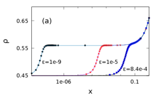
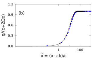
Figure 2: RG solution vs numerical results. (a)Results for $\epsilon=8.4\times 10^{-4},10^{-5},10^{-9}$. Data points are from numerical solutions of Eq. (2) for $r=1,\Omega=0.1,\alpha=0.45$ and $\gamma=0.66$. The RG solution of Eq. (13) are shown by solid lines. (b) Data collapse plot for the same set of data as in (a) (same symbols). Labels show the variables along x and y axes. The solid line is the tanh part of Eq. (13).

III.1 Comparison with numerics

We compare the numerical solution of Eq. (2) for $r=1$, with plots obtained from the RG solution, Eq. (13). In Fig. 2, plots for the high-density phase with the boundary conditions $\alpha=0.45$ and $\gamma=0.66$ are shown. The numerical solutions of the full differential equation for three different $\epsilon$, viz., $\epsilon=8.4\times 10^{-4},10^{-5},10^{-9}$, are shown here. For the RG solution in Eq. (13), the constants $C$ and $x_{0}=\epsilon k$ are found from the boundary conditions at $x=1$ and $x=0$. This is based on the observation that the boundary layer in the high density phase is formed at the $x=0$ boundary. The equations are $C+2\Omega=0.32$ and $C\tanh[Cx_{0}/2\epsilon]=0.1$, yielding $C=0.12$ and $k=4.98$. A nice agreement with the RG solution is seen for the corresponding $\epsilon$’s. Moreover, Eq. (13) admits a scaling form via a collapse of all curves for different $\epsilon$’s if $\phi(x)/(C+2\Omega x)$ is taken as a function of $\tilde{x}=(x-x_{0})/\epsilon$. Such a form is not expected from the naive boundary layer solution. A data collapse plot for all the numerical solutions is shown in Fig. 2b, confirming the predicted scaling.

We also compared the profiles for the shock phase. For a shock phase with $x_{0}$ somewhere in the interior of the lattice, there is a symmetry $\phi(\tilde{x})=-\phi(-\tilde{x})$, obeyed by Eq. (3). We, therefore, concentrate on $\tilde{x}>0$ only. The boundary conditions chosen here are $\alpha=0.3$ and $\gamma=0.7$, so that the shock is formed at $x_{0}=0.5$. Eq. (2) is solved numerically with these boundary conditions. With $x_{0}=0.5$ and the BC at $x=1$, we have $C+2\Omega(x-x_{0})=0.4$, so that $C=0.3$. The symmetry automatically fixes the boundary condition at $x=0$. In this way, the RG analysis performed with boundary layer located near one of the boundaries can be utilized here. A good agreement is noted between the numerical solution of the full differential equation and the RG solution as given in Eq. (13) (see Fig. 3).

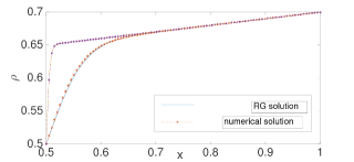
Figure 3: Density profile for shocks. The upper and lower curves correspond to $\epsilon=0.001$, and $0.01$, respectively. The boundary parameters are $\alpha=0.3$ and $\gamma=0.7$. The graph is plotted over the range $x\in[0.5:1]$.

IV Summary

In this paper, we developed a renormalization group scheme to determine the particle density profile in a one-dimensional, particle non-conserving totally asymmetric simple exclusion process. The particle adsorption/desorption kinetics (Langmuir kinetics) is the source of particle non-conservation while the steady state of nonzero current is maintained by the injection and the withdrawal rates at the boundaries. The continuum differential equation for the proocess is singular due to a small prefactor ($\epsilon$) in front of its highest order derivative term that comes from diffusion. As a consequence of the singularity, the perturbative solution on the scale of $\tilde{x}=x/\epsilon$ shows divergences at $O(\epsilon)$ at large distances, $\tilde{x}\to\infty$. Upon absorbing the divergences systematically through renormalizations of the position and the width of the boundary layer, we arrive at a globally valid density-profile which describes both the boundary layer and its crossing over to the bulk solution. One of the predictions of the solution is the appearance of a finite-size scaling form for the density, which compares well with the results from direct numerical solutions of the steady-state differential equation in the high-density and the shock phases. We believe our procedure is general enough to apply to other boundary induced transitions as well.

Appendix A Boundary layer analysis

The differential equation describing the density is given by

$$\epsilon\frac{d^{2}\rho}{dx^{2}}+(2\rho-1)\frac{d\rho}{dx}+\Omega(r-(r+1)\rho)=0.$$ (16)

It is singular due to the small prefactor $\epsilon$ in front of the highest order derivative. In the extreme limit, $\epsilon=0$, the equation reduces to a first order equation which cannot, in general, satisfy two boundary conditions. The loss of a boundary condition leads to the appearance of a boundary layer. The solution of (16) for $\epsilon=0$ describes the major (bulk) part of the density profile and in the language of the boundary layer theory, it is referred as the outer solution. Thus, at zeroth order in $\epsilon$, the possible outer solutions $\rho_{\rm out}$ are

$$\rho_{{\rm out}}=\Omega x+c,\ \ {\rm and}\ \rho_{{\rm out}}=\frac{1}{2},\ {\rm for}\ \ r=1,$$ (17)

while for $r\neq 1$,

$$g(\rho_{\rm out})=\Omega x+c\ {\rm with}$$ (19)

$$g(\rho)=\frac{1}{1+r}{\Big{(}}2\rho+r_{0}\log[r-(r+1)\rho]{\Big{)}}.$$ (20)

Here $r_{0}=\frac{r-1}{r+1}$ and $c$ is the integration constant the value of which can be determined using the boundary conditions. Equation (19) is a transcendental equation which can be solved for $\rho$ numerically. An explicit perturbative solution for $\phi$($=2\rho-1$) in small $r_{0}$ appears as

$$\phi=(\Omega^{\prime}x+c_{0})-r_{0}\log(\Omega^{\prime}x+c_{0}),$$ (21)

where $\Omega^{\prime}=\Omega(r+1)$ and $c_{0}$ is a constant. A boundary layer solution, necessary to account for the other boundary condition, can be found out by introducing a scaled variable $\tilde{x}=\frac{(x-x_{0})}{\epsilon}$, where $x_{0}$ represents the location of the boundary layer. For example, for a boundary layer that appears near $x=1$ boundary, $x_{0}\approx 1$. With this change of the independent variable, equation (16), in terms of $\phi$, appears as

$$\frac{d^{2}\phi}{d\tilde{x}^{2}}+\phi\frac{d\phi}{d\tilde{x}}+\epsilon\Omega^{\prime}(r_{0}-\phi)=0.$$ (22)

In the following, we refer to the solution of this equation as the inner solution ($\phi_{\rm in}$) or boundary layer solution. Upon one integration, the boundary layer equation at the zeroth order in $\epsilon$ is $\frac{d\phi_{\rm in}}{d\tilde{x}}+\frac{\phi_{\rm in}^{2}}{2}=c_{1}=\frac{\phi_{b}^{2}}{2}$ for all $r$. Apart from satisfying a boundary condition, the boundary layer also has to saturate to the outer solution. For satisfying two such conditions, a second order differential equation as (22) is necessary for the description of the boundary layer. The second equality in the differential equation for $\phi_{\rm in}$ ensures that the boundary layer solution saturates to the outer solution $\phi_{b}=2\rho_{b}-1$ with $\rho_{b}$ being the bulk density near the saturation limit. In terms of $\phi_{b}$, the zeroth order inner (boundary layer) solution is

$$\phi_{\rm in}=\phi_{b}\coth[\frac{\phi_{b}}{2}(\tilde{x}+k)],\ {\rm or}\ \phi_{b}\tanh[\frac{\phi_{b}}{2}(\tilde{x}+k)]$$ (23)

where $k$ is the second integration constant. As can be seen from (23), the width of the boundary layer is proportional to $\epsilon$. Thus as $\epsilon\rightarrow 0$, a boundary layer becomes narrower appearing like a jump discontinuity in the density profile. In the low-density phase the density profile has a linear outer or bulk solution along with a boundary layer near $x=1$ ($x_{0}\approx 1$). Since the outer solution, in this case, satisfies the boundary condition at $x=0$, we have $c=\alpha$. The boundary layer, in this case, satisfies the boundary condition at $x=1$ and merges to the bulk profile for $x<1$ i.e for $\tilde{x}\rightarrow-\infty$. The saturation of the boundary layer and the bulk solution is ensured through the matching condition $\rho_{in}(\tilde{x}\rightarrow-\infty)=\rho_{\rm out}(x=1)=\rho_{b}$. For a boundary layer located near $x=0$ boundary (i.e. $x_{0}\approx 0$), the boundary layer saturates to the bulk in the $\tilde{x}\rightarrow\infty$ limit and satisfies the boundary condition at $x=0$. The boundary condition at $x=1$, on the other hand, is satisfied by the outer solution. Density profiles of this shape are seen in the high-density phase which is related to the low-density phase through the particle-hole symmetry. A more drastic behaviour is seen in the shock phase where the boundary layer enters into the interior of the system upon deconfinement from the system boundary. Such a boundary layer joins a low-density type density profile on one side to the high-density type profile on the other side.

Appendix B Details of the RG calculations

At the $O(\epsilon^{0})$ level, we choose the $\tanh$ type solution for $\phi_{0}$. With this, the complete solution for $\phi_{1}$ is

$$\phi_{1}(\tilde{x})=c_{2}\ {\rm sech}^{2}[\frac{p}{2}(k+\tilde{x})]+\frac{1}{4p^{2}}{\rm sech}^{2}[\frac{p}{2}(k+\tilde{x})]{\Bigg{[}}2r_{0}\Omega^{\prime}\cosh[p(k+\tilde{x})]+4\Omega^{\prime}p\ {\rm polylog}[2,-\exp\{-p(k+\tilde{x})\}]-$$

$$p^{2}(k+\tilde{x}){\Big{(}}-2\Omega^{\prime}-r_{0}k\Omega^{\prime}+k\Omega^{\prime}p+r_{0}\Omega^{\prime}\tilde{x}+\Omega^{\prime}p\tilde{x}-2c_{1}+4\Omega^{\prime}\log[1+\exp\{-p(k+\tilde{x})\}]-4\Omega^{\prime}\log[\cosh\{\frac{p}{2}(k+\tilde{x})\}]{\Big{)}}-$$

$$2p{\Big{(}}\Omega^{\prime}+r_{0}\Omega^{\prime}\tilde{x}-c_{1}-2\Omega^{\prime}\log[\cosh\{\frac{1}{2}p(k+\tilde{x})\}]{\Big{)}}\sinh[p(k+\tilde{x})]{\Bigg{]}}.$$ (24)

The terms proportional to $\tilde{x}$ and the $\log[\cosh[...]]$ term in the last part of the above expression are responsible for the breakdown of the perturbation series in the $\epsilon\tilde{x}\rightarrow O(1)$ limit. Writing explicitly the diverging terms, one may write

$$\phi=p\tanh[\frac{p}{2}(k+\tilde{x})]+\epsilon{\Bigg{[}}-\frac{1}{p}\tanh[\frac{p}{2}(k+\tilde{x})]{\Big{(}}\Omega^{\prime}+r_{0}\Omega^{\prime}\tilde{x}-c_{1}-2\Omega^{\prime}\log[\cosh\{\frac{p}{2}(k+\tilde{x})\}]{\Big{)}}{\Bigg{]}}+\epsilon{\cal R},$$ (25)

where ${\cal R}$ represents all the regular terms. Considering the large $\tilde{x}$ limit, we rewrite the above expression as

$$\phi=p\tanh[\frac{p}{2}(k+\tilde{x})]+\epsilon{\Bigg{[}}-\frac{1}{p}\tanh[\frac{p}{2}(k+\tilde{x})]{\Big{(}}r_{0}\Omega^{\prime}\tilde{x}-\Omega^{\prime}p(k+\tilde{x}){\Big{)}}{\Bigg{]}}+\epsilon{\cal R}.$$ (26)

The divergences in the last two terms proportional to $\tilde{x}$ can be isolated by introducing an arbitrary length scale $\mu$. The renormalized parameter is defined through $p_{r}$ as $p=p_{r}+a_{1}\epsilon$ with $a_{1}=\frac{\mu}{p_{r}}(r_{0}-p_{r})\Omega^{\prime}$. Upto $O(\epsilon)$, the divergence free solution becomes

$$\phi = p_{r}\tanh[\frac{p_{r}}{2}(k+\tilde{x})]+\epsilon p_{r}{\rm sech}^{2}[\frac{p_{r}}{2}(k+\tilde{x})]\frac{\mu}{2p_{r}}(r_{0}-p_{r})\Omega^{\prime}-$$ (27)

$$\frac{\epsilon}{p_{r}}\tanh[\frac{p_{r}}{2}(k+\tilde{x})](r_{0}-p_{r})\Omega^{\prime}(\tilde{x}+k-\mu).$$

Next, we impose the condition that $\phi$ must be independent of the arbitrary length scale $\mu$ i.e. $\frac{\partial\phi}{\partial\mu}=0$. Thus, the following expression

$$\frac{\partial\phi}{\partial\mu}=p_{r}^{\prime}(\mu)T_{h}+p_{r}S_{h}p_{r}^{\prime}(\mu)\frac{(k+\tilde{x})}{2}$$

$$-{\epsilon}{\Big{[}}2p_{r}^{\prime}S_{h}T_{h}\ \frac{(k+\tilde{x})^{2}}{4}{\mu}(r_{0}-p_{r})\Omega^{\prime}-S_{h}\frac{(k+\tilde{x})}{2}(r_{0}-p_{r})\Omega^{\prime}+\mu p_{r}^{\prime}\Omega^{\prime}S_{h}\frac{(k+\tilde{x})}{2}{\Big{]}}+$$

$$\epsilon{\Big{[}}\frac{1}{p_{r}^{2}}p_{r}^{\prime}T_{h}\ ((r_{0}-p_{r})\Omega^{\prime}(k+\tilde{x}-\mu))-\frac{1}{p_{r}}p_{r}^{\prime}S_{h}\frac{(k+\tilde{x})}{2}\{(r_{0}-p_{r})\Omega^{\prime}(k+\tilde{x}-\mu)\}-$$

$$\frac{1}{p_{r}}T_{h}\{-p_{r}^{\prime}\Omega^{\prime}(k+\tilde{x}-\mu)-(r_{0}-p_{r})\Omega^{\prime}\}{\Big{]}},$$ (28)

where

$$T_{h}\equiv\tanh\left[\frac{p_{r}}{2}(k+\tilde{x})\right],~{}{\rm and}~{}S_{h}\equiv{\rm sech}^{2}\left[\frac{p_{r}}{2}(k+\tilde{x})\right]$$ (29)

satisfies the required condition if, to $O(\epsilon)$, we have

$$\frac{dp_{r}}{d\mu}=-\frac{\epsilon}{p_{r}}(r_{0}-p_{r})\Omega^{\prime}.$$ (30)

In (28), $p_{r}^{\prime}(\mu)=\frac{dp_{r}}{d\mu}$. Eq. (30) has been solved perturbatively in small $r_{0}$ in the main text.

References

- (1) O. Golinelli, K. Mallick, J. Phys. A: Math. Gen. 39, 12679 (2006).
- (2) T. Liggett, Interacting Particle Systems: Contact, Voter and Exclusion Processes (Springer-Verlag, Berlin, 1999).
- (3) B. Derrida, M. R. Evans, V. Hakim and V. Pasquier, J. Phys. A 26, 1493 (1993).
- (4) C. T. MacDonald, J. H. Gibbs, A. C. Pipkin, Biopolymers 6, 1 (1968).
- (5) C. T. MacDonald, J. H. Gibbs, Biopolymers 7, 707 (1969).
- (6) G. Schuetz and E. Domany, J. Stat. Phys. 72, 277 (1993).
- (7) V. Popkov, A. Rakos, R. D. Willmann, A. B. Kolomeisky, G. M. Schuetz, Phys. Rev. E 67, 066117 (2003).
- (8) S. Mukherji, Phys. Rev. E 79, 041140 (2009).
- (9) M. R. Evans, R. Juhasz and L. Santen Phys. Rev. E 68 026117 (2003).
- (10) A. Parmeggiani, T. Franosch and E. Frey, Phys. Rev. E 70 046101 (2004); see also evans .
- (11) K. E. P. Sugden and M. R. Evans, J. Stat. Mech. P11013 (2007).
- (12) S. Mukherji and S. M. Bhattacharjee, J. Phys. A 38, L285 (2005); S. Mukherji and V. Mishra, Phys. Rev. E 74, 01116 (2006).
- (13) J. D. Cole, Perturbation Methods in Applied Mathematics (Blaisdel Publishing company, Waltham, MA: 1968).
- (14) Lin-Yuan Chen, Nigel Goldenfeld, and Y. Oono, Phys. Rev. E 54, 376 (1996)
- (15) A review on the use of RG theory to singularly perturbed differential equations can also be found in R. E. O’Mallet, Jr. and E. Kirkinis, Studies in applied mathematics 124, 383 (2010).
- (16) J. R. Cash, G. Moore, and R. W. Wright, J. Comp. Phys. 122, 266 (1995).
- (17) J. Krug, Phys. Rev. Lett. 67, 1882 (1991).
- (18) Adsorption (evaporation) at a site can take place only if the site is empty (occupied), i.e. if .
- (19) John Veysey II and Nigel Goldenfeld, Rev. Mod. Phys.79, 883 (2007).