Left-right symmetry, orbifold $S^{1}/Z_{2}$,
and radiative breaking of $U(1)_{\rm R}\times U(1)_{\rm B-L}$

Yugo Abe^a, Yuhei Goto^b and Yoshiharu Kawamura^c

${}^{a}\,$National Institute of Technology, Miyakonojo College, Miyakonojo 885-8567, Japan
${}^{b}\,$Research and Education Center for Natural Science, Keio University, Yokohama 223-8521, Japan
${}^{c}\,$Department of Physics, Shinshu University, Matsumoto 390-8621, Japan

We study the origin of electroweak symmetry under the assumption that $SU(4)_{\rm C}\times SU(2)_{\rm L}\times SU(2)_{\rm R}$ is realized on a five-dimensional space-time. The Pati-Salam type gauge symmetry is reduced to $SU(3)_{\rm C}\times SU(2)_{\rm L}\times U(1)_{\rm R}\times U(1)_{\rm B-L}$ by orbifold breaking mechanism on the orbifold $S^{1}/Z_{2}$. The breakdown of residual gauge symmetries occurs radiatively via the Coleman-Weinberg mechanism, such that the $U(1)_{\rm R}\times U(1)_{\rm B-L}$ symmetry is broken down to $U(1)_{\rm Y}$ by the vacuum expectation value of an $SU(2)_{\rm L}$ singlet scalar field and the $SU(2)_{\rm L}\times U(1)_{\rm Y}$ symmetry is broken down to the electric one $U(1)_{\rm EM}$ by the vacuum expectation value of an $SU(2)_{\rm L}$ doublet scalar field regarded as the Higgs doublet. The negative Higgs squared mass term is originated from an interaction between the Higgs doublet and an $SU(2)_{\rm L}$ singlet scalar field as a Higgs portal. The vacuum stability is recovered due to the contributions from Kaluza-Klein modes of gauge bosons.

1 Introduction

The discovery of the Higgs boson [1, 2], the last piece of the standard model (SM) particles, kicks off a new stage of physics beyond the SM. Mysteries concerning the Higgs boson have thickened because any evidences from new physics such as supersymmetry and compositeness have not been discovered.

One of big mysteries is what the origin of electroweak scale is or how the vacuum expectation value (VEV) of the Higgs boson, $v=246$ GeV, is understood. To unveil the riddle, we need to uncover the origin of Higgs potential, in particular, a mass term therein. Another one is why the vacuum is stable enough after the breakdown of electroweak symmetry. With the Higgs quartic coupling constant $\lambda\doteqdot 0.129$ estimated from the observed Higgs mass $m_{h}\doteqdot 125.1$ GeV, we encounter the vacuum stability problem that $\lambda$ becomes negative at around $10^{7}$ GeV and the vacuum can decay.

In this paper, we tackle these problems through the extensions of gauge symmetries and space-time. Concepts such as simplicity and variety are also adopted on a case-by-case basis. The SM gauge symmetry can be extended to contain a left-right symmetry. A typical one is the gauge group $G_{\rm PS}\equiv SU(4)_{\rm C}\times SU(2)_{\rm L}\times SU(2)_{\rm R}$ in the Pati-Salam model [3]. The space-time can be expanded to include extra dimensions. The orbifold $S^{1}/Z_{2}$ is used as an extra space, because it is simple and has several advantages. Different breaking mechanisms are utilized for the breakdown of gauge symmetry $G_{\rm PS}$ into $SU(3)_{\rm C}\times U(1)_{\rm EM}$, presuming that nature respects diversity.

We give an outline of our model. Particle physics above some high-energy scale $M_{\rm PS}$ is described by a gauge theory with $G_{\rm PS}$ on the five-dimensional (5D) space-time including $S^{1}/Z_{2}$ as an extra dimension. The gauge symmetry $G_{\rm PS}$ is reduced to $G_{3211}\equiv SU(3)_{\rm C}\times SU(2)_{\rm L}\times U(1)_{\rm R}\times U(1)_{\rm B-L}$ by orbifold breaking mechanism. The breakdown of residual gauge symmetries occurs radiatively via the Coleman-Weinberg mechanism. In concrete, the $U(1)_{\rm R}\times U(1)_{\rm B-L}$ symmetry is broken down to $U(1)_{\rm Y}$ by the VEV $v_{\rm R}$ of an $SU(2)_{\rm L}$ singlet scalar field. Then, a gauge boson corresponding to the broken $U(1)$ symmetry acquires a mass $M_{Z_{\rm LR}}$ of $O(v_{\rm R})$. The $SU(2)_{\rm L}\times U(1)_{\rm Y}$ symmetry is broken down to the electric one $U(1)_{\rm EM}$ by the VEV of an $SU(2)_{\rm L}$ doublet scalar field regarded as the Higgs doublet. If the $SU(2)_{\rm L}$ singlet scalar field is replaced by its VEV, we obtain the Higgs potential including a negative squared mass term originated from an interaction between the Higgs doublet and an $SU(2)_{\rm L}$ singlet scalar field as a Higgs portal. The vacuum stability is recovered due to the contributions from Kaluza-Klein modes of gauge bosons appearing at a compactification scale $M_{\rm c}$.

This paper is organized as follows. In the next section, we formulate a 5D Pati-Salam model. We examine the Coleman-Weinberg mechanism and the vacuum stability in a four-dimensional (4D) model with $G_{3211}$ in Sect. 3, In the last section, we give conclusions and discussions.

2 Five-dimensional Pati-Salam model

The space-time is assumed to be factorized into a product of 4D Minkowski space-time $M^{4}$ and the orbifold $S^{1}/Z_{2}$, whose coordinates are denoted by $x^{\mu}$ (or $x$) ($\mu=0,1,2,3$) and $y$, respectively. The 5D notation $x^{M}$ ($M=0,1,2,3,5$) is also used with $x^{5}=y$. The $S^{1}/Z_{2}$ is obtained by dividing the circle $S^{1}$ (with the identification $y\sim y+2\pi R$) by the $Z_{2}$ transformation $y\rightarrow-y$. Then, the point $y$ is identified with $-y$ on $S^{1}/Z_{2}$, and the space is regarded as an interval with length $\pi R$ ($R$ being the radius of $S^{1}$).

In the following, we formulate a Pati-Salam model on $M^{4}\times S^{1}/Z_{2}$. First we present particle contents in Table 1. In most cases, we pay attention to bosons under the assumption that matter fields (quarks and leptons) live on the 4D brane at $y=0$.

Table 1: Gauge quantum numbers of bosons in 5D Pati-Salam model.

bosons	$SU(4)_{\rm C}$	$SU(2)_{\rm L}$	$SU(2)_{\rm R}$
$G_{M}(x,y)$	$\bm{15}$	$\bm{1}$	$\bm{1}$
$W_{{\rm L}M}(x,y)$	$\bm{1}$	$\bm{3}$	$\bm{1}$
$W_{{\rm R}M}(x,y)$	$\bm{1}$	$\bm{1}$	$\bm{3}$
$\varPhi_{\rm L}(x,y)$	${\bm{4}}$	$\bm{2}$	$\bm{1}$
$\varPhi_{\rm R}(x,y)$	$\overline{\bm{4}}$	$\bm{1}$	$\bm{2}$
$\varPhi_{\rm B}(x,y)$	$\bm{1}$	$\bm{2}$	$\bm{2}$

The gauge bosons possess several components such that

$$G_{M}(x,y)=\sum_{a=1}^{15}G_{M}^{a}(x,y)T_{\rm C}^{a},~{}~{}$$ (2.1)

$$W_{{\rm L}M}(x,y)=\sum_{a=1}^{3}W_{{\rm L}M}^{a}(x,y)T_{\rm L}^{a},~{}~{}W_{{\rm R}M}(x,y)=\sum_{a=1}^{3}W_{{\rm R}M}^{a}(x,y)T_{\rm R}^{a},$$

where $T_{\rm C}^{a}$, $T_{\rm L}^{a}$ and $T_{\rm R}^{a}$ are generators of $SU(4)_{\rm C}$, $SU(2)_{\rm L}$ and $SU(2)_{\rm R}$, respectively. We need a scalar field $\varPhi_{\rm B}(x,y)$ that obeys the bi-fundamental representation under $SU(2)_{\rm L}\times SU(2)_{\rm R}$, to construct Yukawa interactions on the brane. The Lagrangian density for bosons is given by

$$\mathscr{L}_{\rm 5D}=-\frac{1}{4}\sum_{a=1}^{15}G_{MN}^{a}G^{aMN}-\frac{1}{4}\sum_{a=1}^{3}W_{{\rm L}MN}^{a}W_{\rm L}^{aMN}-\frac{1}{4}\sum_{a=1}^{3}W_{{\rm R}MN}^{a}W_{\rm R}^{aMN}$$ (2.2)

$$~{}~{}~{}~{}~{}~{}~{}~{}~{}+(D_{M}\varPhi_{\rm L})^{\dagger}(D^{M}\varPhi_{\rm L})+(D_{M}\varPhi_{\rm R})^{\dagger}(D^{M}\varPhi_{\rm R})+{\rm tr}(D_{M}\varPhi_{\rm B})^{\dagger}(D^{M}\varPhi_{\rm B})-V_{\rm 5D},$$

where $G_{MN}^{a}$, $W_{{\rm L}MN}^{a}$ and $W_{{\rm R}MN}^{a}$ are field strengths of $SU(4)_{\rm C}$, $SU(2)_{\rm L}$ and $SU(2)_{\rm R}$ gauge bosons, respectively. The covariant derivative $D_{M}$ and the scalar potential $V_{\rm 5D}$ are given by

$$D_{M}=\partial_{M}+ig_{4}\sum_{a=1}^{15}G_{M}^{a}T_{\rm C}^{a}+ig_{\rm L}\sum_{a=1}^{3}W_{{\rm L}M}^{a}T_{\rm L}^{a}+ig_{\rm R}\sum_{a=1}^{3}W_{{\rm R}M}^{a}T_{\rm R}^{a},$$

$$V_{\rm 5D}=\lambda_{\rm L}|\varPhi_{\rm L}|^{4}+\lambda_{\rm R}|\varPhi_{\rm R}|^{4}+\lambda_{\rm B1}{\rm tr}\left(|\varPhi_{\rm B}|^{2}|\varPhi_{\rm B}|^{2}\right)+\lambda_{\rm B2}\left({\rm tr}|\varPhi_{\rm B}|^{2}\right)^{2}$$

$$~{}~{}~{}~{}~{}+\lambda_{\rm LR}|\varPhi_{\rm L}|^{2}|\varPhi_{\rm R}|^{2}+\lambda_{\rm LB}|\varPhi_{\rm L}|^{2}{\rm tr}|\varPhi_{\rm B}|^{2}+\lambda_{\rm RB}|\varPhi_{\rm R}|^{2}{\rm tr}|\varPhi_{\rm B}|^{2},$$ (2.4)

respectively. If we require the left-right symmetry that the theory should be invariant under the exchange $(W_{{\rm L}M}^{a},\varPhi_{\rm L})$ into $(W_{{\rm R}M}^{a},\varPhi_{\rm R})$, we obtain the conditions among couplings:

$$g_{\rm L}=g_{\rm R},~{}~{}\lambda_{\rm L}=\lambda_{\rm R},~{}~{}\lambda_{\rm LB}=\lambda_{\rm RB}.$$ (2.5)

We suppose that all scalar fields have no bulk masses.

From the requirement that the Lagrangian density should be invariant under the translation $T:y\to y+2\pi R$ and the $Z_{2}$ transformation $P_{0}:y\to-y$ or it should be a single-valued function on the 5D space-time, non-trivial boundary conditions (BCs) of fields are allowed on $S^{1}/Z_{2}$.

We impose the following BCs on $G_{M}$,

$$G_{\mu}(x,-y)=G_{\mu}(x,y),~{}~{}G_{5}(x,-y)=-G_{5}(x,y),$$ (2.6)

$$G_{\mu}(x,2\pi R-y)=U_{\rm C}G_{\mu}(x,y)U_{\rm C}^{-1},~{}~{}G_{5}(x,2\pi R-y)=-U_{\rm C}G_{5}(x,y)U_{\rm C}^{-1},$$ (2.7)

where $U_{\rm C}={\rm diag}(1,1,1,-1)$. We use the $Z_{2}$ transformation $P_{1}:y\to 2\pi R-y$ in place of $T:y\to y+2\pi R$. Then, $G_{M}$ are given by the Fourier expansions:

$$G_{\mu}^{a}(x,y)=\frac{1}{\sqrt{2\pi{R}}}G_{\mu}^{(0)a}(x)+\frac{1}{\sqrt{\pi{R}}}\sum_{n=1}^{\infty}G_{\mu}^{(n)a}(x)\cos\frac{ny}{R}~{}~{}~{}(a=1,\cdots,8,15),$$ (2.8)

$$G_{\mu}^{a}(x,y)=\frac{1}{\sqrt{\pi{R}}}\sum_{n=1}^{\infty}G_{\mu}^{(n)a}(x)\cos\frac{\left(n-\frac{1}{2}\right)y}{R}~{}~{}~{}(a=9,\cdots,14),$$ (2.9)

$$G_{5}^{a}(x,y)=\frac{1}{\sqrt{\pi{R}}}\sum_{n=1}^{\infty}G_{5}^{(n)a}(x)\sin\frac{ny}{R}~{}~{}~{}(a=1,\cdots,8,15),$$ (2.10)

$$G_{5}^{a}(x,y)=\frac{1}{\sqrt{\pi{R}}}\sum_{n=1}^{\infty}G_{5}^{(n)a}(x)\sin\frac{\left(n-\frac{1}{2}\right)y}{R}~{}~{}~{}(a=9,\cdots,14).$$ (2.11)

Only $G_{\mu}^{a}$ ($a=1,\cdots,8,15$) have $y$-independent modes with $n=0$ called zero modes, and $G_{\mu}^{(0)a}(x)$ ($a=1,\cdots,8$) and $G_{\mu}^{(0)15}(x)$ are identified as the 4D gluons and the 4D $U(1)_{\rm B-L}$ gauge boson, respectively. We denote them as $G_{\mu}^{a}(x)$ and $N_{\mu}(x)$, respectively.

We impose the following BCs on $W_{{\rm L}M}$,

$$W_{{\rm L}\mu}(x,-y)=W_{{\rm L}\mu}(x,y),~{}~{}W_{{\rm L}5}(x,-y)=-W_{{\rm L}5}(x,y),$$ (2.12)

$$W_{{\rm L}\mu}(x,2\pi R-y)=W_{{\rm L}\mu}(x,y),~{}~{}W_{{\rm L}5}(x,2\pi R-y)=-W_{{\rm L}5}(x,y)$$ (2.13)

and then we obtain the zero modes $W_{{\rm L}\mu}^{(0)a}(x)$ ($a=1,2,3$) identified as the 4D $SU(2)_{\rm L}$ weak bosons and denote them as $W_{\mu}^{a}(x)$.

We impose the following BCs on $W_{{\rm R}M}$,

$$W_{{\rm R}\mu}(x,-y)=W_{{\rm R}\mu}(x,y),~{}~{}W_{{\rm R}5}(x,-y)=-W_{{\rm R}5}(x,y),$$ (2.14)

$$W_{{\rm R}\mu}(x,2\pi R-y)=U_{\rm R}W_{{\rm R}\mu}(x,y)U_{\rm R}^{-1},~{}~{}W_{{\rm R}5}(x,2\pi R-y)=-U_{\rm R}W_{{\rm R}5}(x,y)U_{\rm R}^{-1},$$ (2.15)

where $U_{\rm R}={\rm diag}(1,-1)$. Then, we obtain the zero modes $W_{{\rm R}\mu}^{(0)3}(x)$ regarded as a $U(1)$ gauge boson. We denote $W_{{\rm R}\mu}^{(0)3}(x)$ and its $U(1)$ gauge group as $R_{\mu}(x)$ and $U(1)_{\rm R}$, respectively.

For scalar fields, the following BCs are imposed on,

$$\varPhi_{\rm L}(x,-y)=-\varPhi_{\rm L}(x,y),~{}~{}\varPhi_{\rm L}(x,2\pi R-y)=-U_{\rm C}\varPhi_{\rm L}(x,y),$$ (2.16)

$$\varPhi_{\rm R}(x,-y)=-U_{\rm R}\varPhi_{\rm R}(x,y),~{}~{}\varPhi_{\rm R}(x,2\pi R-y)=-U_{\rm C}\varPhi_{\rm R}(x,y),$$ (2.17)

$$\varPhi_{\rm B}(x,-y)=\varPhi_{\rm B}(x,y),~{}~{}\varPhi_{\rm B}(x,2\pi R-y)=U_{\rm R}\varPhi_{\rm B}(x,y).$$ (2.18)

Then, zero modes appear from the lower component of $\varPhi_{\rm R}$ and the upper component of $\varPhi_{\rm B}$ concerning $SU(2)_{\rm R}$, and they are denoted as $\phi_{\rm R}(x)$ and $\phi(x)$, respectively. Here, $\phi_{\rm R}(x)$ is the $SU(2)_{\rm L}$ singlet scalar field and $\phi(x)$ is the $SU(2)_{\rm L}$ doublet scalar field. The $\phi(x)$ is regarded as the Higgs doublet in the SM.

We list gauge quantum numbers and mass spectra of bosons after compactification in Table 2.

Table 2: Gauge quantum numbers of bosons after compactification in 5D Pati-Salam model.

bosons	$SU(3)_{\rm C}$	$SU(2)_{\rm L}$	$Q_{\rm R}$	$Q_{\rm B-L}$	$(P_{0},P_{1})$	mass
$G_{\mu}^{(n)a}(x,y)$ $(a=1\sim 8)$	$\bm{8}$	$\bm{1}$	$0$	$0$	$(+1,+1)$	$\frac{n}{R}$
$G_{\mu}^{(n)a}(x,y)$ $(a=9\sim 14)$	$\bm{3}$	$\bm{1}$	$0$	$\frac{2}{3}$	$(+1,-1)$	$\frac{n-\frac{1}{2}}{R}$
	$\overline{\bm{3}}$	$\bm{1}$	$0$	$-\frac{2}{3}$	$(+1,-1)$	$\frac{n-\frac{1}{2}}{R}$
$G_{\mu}^{(n)15}(x,y)$	$\bm{1}$	$\bm{1}$	$0$	$0$	$(+1,+1)$	$\frac{n}{R}$
$W_{{\rm L}\mu}^{(n)a}(x,y)$ $(a=1,2,3)$	$\bm{1}$	$\bm{3}$	0	$0$	$(+1,+1)$	$\frac{n}{R}$
$W_{{\rm R}\mu}^{(n)3}(x,y)$	$\bm{1}$	$\bm{1}$	$0$	$0$	$(+1,+1)$	$\frac{n}{R}$
$W_{{\rm R}\mu}^{(n)+}(x,y)$	$\bm{1}$	$\bm{1}$	$1$	$0$	$(+1,-1)$	$\frac{n-\frac{1}{2}}{R}$
$W_{{\rm R}\mu}^{(n)-}(x,y)$	$\bm{1}$	$\bm{1}$	$-1$	$0$	$(+1,-1)$	$\frac{n-\frac{1}{2}}{R}$
$G_{5}^{(n)a}(x,y)$ $(a=1\sim 8)$	$\bm{8}$	$\bm{1}$	$0$	$0$	$(-1,-1)$	$\frac{n}{R}$
$G_{5}^{(n)a}(x,y)$ $(a=9\sim 14)$	$\bm{3}$	$\bm{1}$	$0$	$\frac{2}{3}$	$(-1,+1)$	$\frac{n-\frac{1}{2}}{R}$
	$\overline{\bm{3}}$	$\bm{1}$	$0$	$-\frac{2}{3}$	$(-1,+1)$	$\frac{n-\frac{1}{2}}{R}$
$G_{5}^{(n)15}(x,y)$	$\bm{1}$	$\bm{1}$	$0$	$0$	$(-1,-1)$	$\frac{n}{R}$
$W_{{\rm L}5}^{(n)a}(x,y)$ $(a=1,2,3)$	$\bm{1}$	$\bm{3}$	0	$0$	$(-1,-1)$	$\frac{n}{R}$
$W_{{\rm R}5}^{(n)3}(x,y)$	$\bm{1}$	$\bm{1}$	$0$	$0$	$(-1,-1)$	$\frac{n}{R}$
$W_{{\rm R}5}^{(n)+}(x,y)$	$\bm{1}$	$\bm{1}$	$1$	$0$	$(-1,+1)$	$\frac{n-\frac{1}{2}}{R}$
$W_{{\rm R}5}^{(n)-}(x,y)$	$\bm{1}$	$\bm{1}$	$-1$	$0$	$(-1,+1)$	$\frac{n-\frac{1}{2}}{R}$
$\varPhi_{\rm L}(x,y)$	${\bm{3}}$	$\bm{2}$	$0$	$\frac{1}{6}$	$(-1,-1)$	$\frac{n}{R}$
	$\bm{1}$	$\bm{2}$	$0$	$-\frac{1}{2}$	$(-1,+1)$	$\frac{n-\frac{1}{2}}{R}$
$\varPhi_{\rm R}(x,y)$	$\overline{\bm{3}}$	$\bm{1}$	$\frac{1}{2}$	$-\frac{1}{6}$	$(-1,-1)$	$\frac{n}{R}$
	$\overline{\bm{3}}$	$\bm{1}$	$-\frac{1}{2}$	$-\frac{1}{6}$	$(+1,-1)$	$\frac{n-\frac{1}{2}}{R}$
	$\bm{1}$	$\bm{1}$	$\frac{1}{2}$	$\frac{1}{2}$	$(-1,+1)$	$\frac{n-\frac{1}{2}}{R}$
	$\bm{1}$	$\bm{1}$	$-\frac{1}{2}$	$\frac{1}{2}$	$(+1,+1)$	$\frac{n}{R}$
$\varPhi_{\rm B}(x,y)$	$\bm{1}$	$\bm{2}$	$\frac{1}{2}$	$0$	$(+1,+1)$	$\frac{n}{R}$
	$\bm{1}$	$\bm{2}$	$-\frac{1}{2}$	$0$	$(+1,-1)$	$\frac{n-\frac{1}{2}}{R}$

In Table 2, $Q_{\rm R}$ is the $U(1)_{\rm R}$ charge and $Q_{\rm B-L}$ is the $U(1)_{\rm B-L}$ charge defined by

$$Q_{\rm B-L}\equiv\sqrt{\frac{2}{3}}T_{\rm C}^{15},$$ (2.19)

using the 15-th components of $T_{\rm C}^{a}$. The fifth components of gauge bosons are would-be Nambu-Goldstone bosons and absorbed by the corresponding 4D gauge bosons.

After the dimensional reduction, we obtain the Lagrangian density:

$$\mathscr{L}_{\rm 4D}=-\frac{1}{4}\sum_{a=1}^{8}G_{\mu\nu}^{a}G^{a\mu\nu}-\frac{1}{4}\sum_{a=1}^{3}W_{\mu\nu}^{a}W^{a\mu\nu}-\frac{1}{4}R_{\mu\nu}R^{\mu\nu}-\frac{1}{4}N_{\mu\nu}N^{\mu\nu}$$ (2.20)

$$~{}~{}~{}~{}~{}~{}~{}~{}~{}+(D_{\mu}\phi_{\rm R})^{\dagger}(D^{\mu}\phi_{\rm R})+(D_{\mu}\phi)^{\dagger}(D^{\mu}\phi)-V_{\rm 4D}+\mathscr{L}_{\rm KK},$$

where $G_{\mu\nu}^{a}$, $W_{\mu\nu}^{a}$, $R_{\mu\nu}$ and $N_{\mu\nu}$ are field strengths of $SU(3)_{\rm C}$, $SU(2)_{\rm L}$, $U(1)_{\rm R}$ and $U(1)_{\rm B-L}$ gauge bosons, and $\mathscr{L}_{\rm KK}$ is the Lagrangian density containing Kaluza-Klein modes. Here, the covariant derivative $D_{\mu}$ and the scalar potential $V_{\rm 4D}$ are given by

$$D_{\mu}=\partial_{\mu}+ig_{3}\sum_{a=1}^{8}G_{\mu}^{a}T_{\rm C}^{a}+ig\sum_{a=1}^{3}W_{\mu}^{a}T_{\rm L}^{a}+ig_{\rm R}R_{\mu}Q_{\rm R}+ig_{\rm B-L}N_{\mu}Q_{\rm B-L},$$ (2.21)

$$V_{\rm 4D}=\lambda_{\rm r}|\phi_{\rm R}|^{4}+\lambda|\phi|^{4}+\lambda_{\rm m}|\phi_{\rm R}|^{2}|\phi|^{2},$$ (2.22)

respectively. From the matching conditions between $\mathscr{L}_{\rm 5D}$ and $\mathscr{L}_{\rm 4D}$ at a scale $M_{\rm PS}$ above the compactification scale $M_{\rm c}(=1/R)$, we obtain the relations:

$$\left.g_{3}=\sqrt{\frac{2}{3}}g_{\rm B-L}=g_{4}\right|_{M_{\rm PS}},~{}~{}\left.g=g_{\rm L}=g_{\rm R}\right|_{M_{\rm PS}},~{}~{}$$ (2.23)

$$\left.\lambda_{\rm r}=\lambda_{\rm R}\right|_{M_{\rm PS}},~{}~{}\left.\lambda=\lambda_{\rm B1}+\lambda_{\rm B2}\right|_{M_{\rm PS}},~{}~{}\left.\lambda_{\rm m}=\lambda_{\rm RB}\right|_{M_{\rm PS}}.$$ (2.24)

Note that fields from zero modes are massless at $M_{\rm PS}$ and the value of $\lambda_{\rm r}$ does not necessarily agree with that of $\lambda$ there.

3 $SU(3)_{\rm C}\times SU(2)_{\rm L}\times U(1)_{\rm R}\times U(1)_{\rm B-L}$ model

Let us study 4D model with the gauge group $SU(3)_{\rm C}\times SU(2)_{\rm L}\times U(1)_{\rm R}\times U(1)_{\rm B-L}$ described by (2.20). We refer to it as 3211 model. Particle contents of massless fields are listed in Table 3.

Table 3: Gauge quantum numbers of massless fields in 4D 3211 model.

particles	$SU(3)_{\rm C}$	$SU(2)_{\rm L}$	$Q_{\rm R}$	$Q_{\rm B-L}$	$Y$	$Y_{\perp}$
$G_{\mu}$	$\bm{8}$	$\bm{1}$	$0$	$0$	$0$	$0$
$W_{\mu}$	$\bm{1}$	$\bm{3}$	$0$	$0$	$0$	$0$
$R_{\mu}$	$\bm{1}$	$\bm{1}$	$0$	$0$	$0$	$0$
$N_{\mu}$	$\bm{1}$	$\bm{1}$	$0$	$0$	$0$	$0$
$\phi_{\rm R}$	$\bm{1}$	$\bm{1}$	$-\frac{1}{2}$	$\frac{1}{2}$	$0$	$\frac{5}{2}$
$\phi$	$\bm{1}$	$\bm{2}$	$\frac{1}{2}$	$0$	$\frac{1}{2}$	$-1$
$q_{{\rm L}A}$	$\bm{3}$	$\bm{2}$	$0$	$\frac{1}{6}$	$\frac{1}{6}$	$\frac{1}{2}$
$u_{{\rm R}A}$	$\bm{3}$	$\bm{1}$	$\frac{1}{2}$	$\frac{1}{6}$	$\frac{2}{3}$	$-\frac{1}{2}$
$d_{{\rm R}A}$	$\bm{3}$	$\bm{1}$	$-\frac{1}{2}$	$\frac{1}{6}$	$-\frac{1}{3}$	$\frac{3}{2}$
$l_{{\rm L}A}$	$\bm{1}$	$\bm{2}$	$0$	$-\frac{1}{2}$	$-\frac{1}{2}$	$-\frac{3}{2}$
$\nu_{{\rm R}A}$	$\bm{1}$	$\bm{1}$	$\frac{1}{2}$	$-\frac{1}{2}$	$0$	$-\frac{5}{2}$
$e_{{\rm R}A}$	$\bm{1}$	$\bm{1}$	$-\frac{1}{2}$	$-\frac{1}{2}$	$-1$	$-\frac{1}{2}$

In Table 3, the subscript $A$ represents the generation of matter fields on the 4D brane and runs from 1 to 3. For a sake of reference, we denote values of the weak hypercharge defined by $Y\equiv Q_{\rm R}+Q_{\rm B-L}$ and those of the $U(1)$ charge defined by $Y_{\perp}\equiv 5Q_{\rm B-L}-2Y$, which is orthogonal to $Y$.

3.1 Running of gauge couplings

We study the running of gauge couplings. By solving the renormalization group equations (RGEs) of gauge couplings $g_{i}$ at the one-loop level, we obtain the solutions,

$$\alpha_{i}^{-1}(\mu)=\alpha_{i}^{-1}(\mu_{0})-\frac{b_{i}}{2\pi}\ln\frac{\mu}{\mu_{0}}$$ (3.1)

$$~{}~{}~{}~{}~{}~{}~{}~{}~{}~{}~{}~{}-\sum_{n=1}\frac{b^{\prime}_{i}}{2\pi}\theta\left(\mu-\frac{n}{R}\right)\ln\frac{\mu}{\frac{n}{R}}-\sum_{n=1}\frac{b^{\prime\prime}_{i}}{2\pi}\theta\left(\mu-\frac{n-\frac{1}{2}}{R}\right)\ln\frac{\mu}{\frac{n-\frac{1}{2}}{R}}$$

where $\alpha_{i}\equiv g_{i}^{2}/(4\pi)$, $\mu$ is a renormalization point, $b_{i}$ are coefficients of $\beta$ functions for zero modes, and $b^{\prime}_{i}$ and $b^{\prime\prime}_{i}$ are coefficients of $\beta$ functions for Kaluza-Klein modes with masses $n/R$ and $(n-\frac{1}{2})/R$, respectively. The $\theta$ is a step function defined by $\theta(x)=1$ for $x>0$, $\theta(x)=0$ for $x<0$ and $\theta(0)=1/2$. The values of $b_{i}$, $b^{\prime}_{i}$ and $b^{\prime\prime}_{i}$ are listed in Table 4.

Table 4: Gauge couplings and their coefficients of $\beta$ functions.

	$SU(3)_{\rm C}$	$SU(2)_{\rm L}$	$U(1)_{\rm R}$	$U(1)_{\rm B-L}$	$U(1)_{\rm Y}$
$g_{i}$	$g_{3}$	$g$	$g_{\rm R}$	$g_{\rm B-L}$	$g_{\rm Y}$
$\alpha_{i}$	$\alpha_{3}$	$\alpha_{2}$	$\alpha_{\rm R}$	$\alpha_{\rm B-L}$	$\alpha_{\rm Y}$
$b_{i}$	$-7$	$-\frac{19}{6}$	$\frac{17}{4}$	$\frac{11}{4}$	$\frac{41}{6}$
$b^{\prime}_{i}$	$-1$	$-\frac{1}{3}$	$\frac{1}{2}$	$\frac{1}{6}$	–
$b^{\prime\prime}_{i}$	$-\frac{1}{3}$	$\frac{1}{3}$	$-\frac{1}{2}$	$-\frac{19}{18}$	–

In Table 4, we list $b_{\rm Y}=41/6$ in the SM for a sake of completeness, and – represents not applicable.

By taking $M_{\rm PS}=n_{\varLambda}/R=n_{\varLambda}M_{\rm c}$ as $\mu$, solutions are written by

$$\alpha_{i}^{-1}(M_{\rm PS})=\alpha_{i}^{-1}(\mu_{0})-\frac{b_{i}}{2\pi}\ln\frac{M_{\rm PS}}{\mu_{0}}-\sum_{n=1}^{n_{\varLambda}}\frac{b^{\prime}_{i}}{2\pi}\ln\frac{M_{\rm PS}}{\frac{n}{R}}-\sum_{n=1}^{n_{\varLambda}}\frac{b^{\prime\prime}_{i}}{2\pi}\ln\frac{M_{\rm PS}}{\frac{n-\frac{1}{2}}{R}}$$ (3.2)

$$~{}~{}~{}~{}~{}~{}~{}~{}~{}~{}~{}~{}~{}=\alpha_{i}^{-1}(\mu_{0})-\frac{b_{i}}{2\pi}\ln\frac{M_{\rm PS}}{\mu_{0}}-\frac{b^{\prime}_{i}}{2\pi}\ln\prod_{n=1}^{n_{\varLambda}}\left(\frac{M_{\rm PS}}{nM_{\rm c}}\right)-\frac{b^{\prime\prime}_{i}}{2\pi}\ln\prod_{n=1}^{n_{\varLambda}}\left(\frac{M_{\rm PS}}{\left(n-\frac{1}{2}\right)M_{\rm c}}\right)$$

$$~{}~{}~{}~{}~{}~{}~{}~{}~{}~{}~{}~{}~{}=\alpha_{i}^{-1}(\mu_{0})-\frac{b_{i}}{2\pi}\ln\frac{M_{\rm PS}}{\mu_{0}}$$

$$~{}~{}~{}~{}~{}~{}~{}~{}~{}~{}~{}~{}~{}~{}~{}~{}-\frac{b^{\prime}_{i}}{2\pi}\left(\frac{M_{\rm PS}}{M_{\rm c}}\ln\frac{M_{\rm PS}}{M_{\rm c}}-\ln\varGamma\left(\frac{M_{\rm PS}}{M_{\rm c}}+1\right)\right)$$

$$~{}~{}~{}~{}~{}~{}~{}~{}~{}~{}~{}~{}~{}~{}~{}~{}-\frac{b^{\prime\prime}_{i}}{2\pi}\left(\frac{M_{\rm PS}}{M_{\rm c}}\ln\frac{M_{\rm PS}}{M_{\rm c}}-\ln\varGamma\left(\frac{M_{\rm PS}}{M_{\rm c}}+\frac{1}{2}\right)+\ln\sqrt{\pi}\right),$$

where $\varGamma$ is a gamma function defined by

$$\varGamma(z)=\int_{0}^{\infty}t^{z-1}e^{-t}dt$$ (3.3)

and we replace $\Pi_{n=1}^{n_{\varLambda}}n=n_{\varLambda}!$ and $\Pi_{n=1}^{n_{\varLambda}}\left(n-\frac{1}{2}\right)=(2n_{\varLambda}-1)!!/2^{n_{\varLambda}}$ into $\varGamma(n_{\varLambda}+1)$ and $\varGamma\left(n_{\varLambda}+\frac{1}{2}\right)/\sqrt{\pi}$, respectively.

From the matching conditions at $M_{\rm PS}$ and $M_{Z_{\rm LR}}$, we have the conditions:

$$\left.\alpha_{3}=\frac{2}{3}\alpha_{\rm B-L}\right|_{M_{\rm PS}},~{}~{}\left.\alpha_{2}=\alpha_{\rm R}\right|_{M_{\rm PS}},~{}~{}\left.\alpha_{\rm Y}^{-1}=\alpha_{\rm R}^{-1}+\alpha_{\rm B-L}^{-1}\right|_{M_{Z_{\rm LR}}},$$ (3.4)

where $M_{Z_{\rm LR}}$ is the mass of gauge boson that becomes massive with the breakdown of $U(1)_{\rm R}\times U(1)_{\rm B-L}$ into $U(1)_{\rm Y}$. By combining with the solutions (3.2), we obtain the sum rule:

$${\alpha}_{\rm Y}^{-1}(M_{Z})-\alpha_{2}^{-1}(M_{Z})-\frac{2}{3}\alpha_{3}^{-1}(M_{Z})$$ (3.5)

$$~{}~{}=\frac{b_{\rm Y}-b_{2}-\frac{2}{3}b_{3}}{2\pi}\ln\frac{M_{\rm PS}}{M_{Z}}+\frac{-b_{\rm Y}+b_{\rm R}+b_{\rm B-L}}{2\pi}\ln\frac{M_{\rm PS}}{M_{Z_{\rm LR}}},$$

$$~{}~{}~{}~{}+\frac{-b^{\prime}_{\rm Y}-\frac{2}{3}b^{\prime}_{3}+b^{\prime}_{\rm R}+b^{\prime}_{\rm B-L}}{2\pi}\left(\frac{M_{\rm PS}}{M_{\rm c}}\ln\frac{M_{\rm PS}}{M_{\rm c}}-\ln\varGamma\left(\frac{M_{\rm PS}}{M_{\rm c}}+1\right)\right)$$

$$~{}~{}~{}~{}+\frac{-b^{\prime\prime}_{\rm Y}-\frac{2}{3}b^{\prime\prime}_{3}+b^{\prime\prime}_{\rm R}+b^{\prime\prime}_{\rm B-L}}{2\pi}\left(\frac{M_{\rm PS}}{M_{\rm c}}\ln\frac{M_{\rm PS}}{M_{\rm c}}-\ln\varGamma\left(\frac{M_{\rm PS}}{M_{\rm c}}+\frac{1}{2}\right)+\ln\sqrt{\pi}\right),$$

where $M_{Z}$ is the $Z$ boson mass given by $M_{Z}\doteqdot 91.19$GeV. Using the values of ($b_{i}$, $b^{\prime}_{i}$, $b^{\prime\prime}_{i}$) and the experimental values such that [25]

$$\alpha_{3}^{-1}(M_{Z})\doteqdot 8.467,~{}~{}\alpha_{2}^{-1}(M_{Z})\doteqdot 29.59,~{}~{}\alpha_{\rm Y}^{-1}(M_{Z})\doteqdot 98.36,$$ (3.6)

we obtain the relation:

$$M_{\rm PS}\doteqdot 3.675\times 10^{13}\times(1.026)^{\xi}\times\left(\frac{\sqrt{\pi}\varGamma(10^{\eta}+1)}{\varGamma(10^{\eta}+\frac{1}{2})}\right)^{0.1124}~{}{\rm GeV},$$ (3.7)

where $M_{Z_{\rm LR}}$ and $M_{\rm PS}$ are parametrized as $M_{Z_{\rm LR}}=10^{\xi}\times M_{Z}$ and $M_{\rm PS}=10^{\eta}\times M_{\rm c}$, respectively. The factor including gamma functions represents contributions from Kaluza-Klein modes. From (3.7), we find the interesting feature that the magnitude of $M_{\rm PS}$ is $O(10^{13})$ GeV almost irrelevant to the value of $M_{Z_{\rm LR}}$. This is due to an accidental fact that the coefficient of the second term in the right hand side of (3.5) is tiny, i.e., $(-b_{\rm Y}+b_{\rm R}+b_{\rm B-L})/(2\pi)\doteqdot 0.02654$. Further, the magnitude of $M_{\rm PS}$ is almost irrelevant to the value of $M_{\rm c}$, because Kaluza-Klein modes appear as complete multiplets (although there is a mass difference with $1/(2R)$) with $(2/3)\times(b^{\prime}_{3}+b^{\prime\prime}_{3})=b^{\prime}_{\rm B-L}+b^{\prime\prime}_{\rm B-L}=-8/9$ and $b^{\prime}_{2}+b^{\prime\prime}_{2}=b^{\prime}_{\rm R}+b^{\prime\prime}_{\rm R}=0$. These features are understood from the $\xi$-$\eta$ plot satisfying (3.7) given in Figure 1.

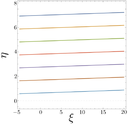
Figure 1: Allowed values of $\xi$ and $\eta$. The colored lines represent the allowed values for $M_{\rm c}=10^{7}$, $10^{8}$, $10^{9}$, $10^{10}$, $10^{11}$, $10^{12}$ and $10^{13}$ GeV from the above.

Typical runnings of $\alpha_{i}^{-1}$ are depicted in Figure 2.

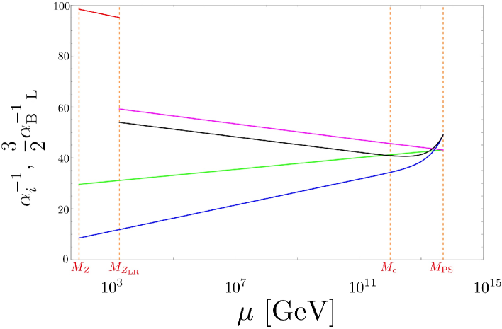
Figure 2: The running of gauge couplings. The red, green, blue, violet and black lines stand for the evolution of $\alpha_{\rm Y}^{-1}$, $\alpha_{2}^{-1}$, $\alpha_{3}^{-1}$, $\alpha_{\rm R}^{-1}$ and $3\alpha_{\rm B-L}^{-1}/2$, respectively.

Here we choose $\xi=1.3$, i.e., $M_{Z_{\rm LR}}\doteqdot 1819$ GeV, and $M_{\rm c}=1\times 10^{12}$ GeV, i.e., $\eta\doteqdot 1.7$, as a bench mark.

3.2 Scalar potential in 3211 model

We study the breakdown of $U(1)_{\rm R}\times U(1)_{\rm B-L}$ and the electroweak symmetry. The scalar potential at the tree level is given by $V_{\rm 4D}$ in (2.22). The quartic couplings $\lambda_{\rm r}$, $\lambda_{\rm m}$, $\lambda$ and the top Yukawa coupling $y_{t}$ obey the RGEs at the one-loop level,

$$\frac{d\lambda_{\rm r}}{d\ln\mu}=\frac{1}{16\pi^{2}}\biggl{(}20\lambda_{\rm r}^{2}+2\lambda_{\rm m}^{2}-3g_{\rm R}^{2}\lambda_{\rm r}-3g_{\rm B-L}^{2}\lambda_{\rm r}$$

$$~{}~{}~{}~{}~{}~{}~{}~{}~{}~{}\left.+\frac{3}{8}g_{\rm R}^{4}+\frac{3}{4}g_{\rm R}^{2}g_{\rm B-L}^{2}+\frac{3}{8}g_{\rm B-L}^{4}\right),$$

$$\frac{d\lambda_{\rm m}}{d\ln\mu}=\frac{1}{16\pi^{2}}\left(4\lambda_{\rm m}^{2}+8\lambda_{\rm r}\lambda_{\rm m}+12\lambda\lambda_{\rm m}-\frac{9}{2}g^{2}\lambda_{\rm m}-3g_{\rm R}^{2}\lambda_{\rm m}\right.$$

$$~{}~{}~{}~{}~{}~{}~{}~{}~{}~{}\left.-\frac{3}{2}g_{\rm B-L}^{2}\lambda_{\rm m}+6y_{t}^{2}\lambda_{\rm m}+\frac{3}{8}g_{\rm R}^{4}\right),$$

$$\frac{d\lambda}{d\ln\mu}=\frac{1}{16\pi^{2}}\left(24\lambda^{2}+\lambda_{\rm m}^{2}-3g_{\rm R}^{2}\lambda-9g^{2}\lambda+\frac{3}{8}g_{\rm R}^{4}+\frac{3}{4}g_{\rm R}^{2}g^{2}\right.$$

$$~{}~{}~{}~{}~{}~{}~{}~{}~{}~{}\left.+\frac{9}{8}g^{4}+12y_{t}^{2}\lambda-6y_{t}^{4}\right),$$ (3.10)

$$\frac{dy_{t}}{d\ln\mu}=\frac{1}{16\pi^{2}}\left(\frac{9}{2}y_{t}^{3}-\frac{3}{4}g_{\rm R}^{2}y_{t}-\frac{1}{6}g_{\rm B-L}^{2}y_{t}-\frac{9}{4}g^{2}y_{t}-8g_{3}^{2}y_{t}\right),$$ (3.11)

where the contributions from Kaluza-Klein modes are omitted.

For a sake of completeness, we write down the RGEs of the Higgs quartic coupling $\lambda$ and the top Yukawa coupling $y_{t}$ in the SM,

$$\frac{d\lambda}{d\ln\mu}=\frac{1}{16\pi^{2}}\biggl{(}24\lambda^{2}-3g_{\rm Y}^{2}\lambda-9g^{2}\lambda$$ (3.12)

$$~{}~{}~{}~{}~{}~{}~{}~{}~{}\left.+\frac{3}{8}g_{\rm Y}^{4}+\frac{3}{4}g_{\rm Y}^{2}g^{2}+\frac{9}{8}g^{4}+12y_{t}^{2}\lambda-6y_{t}^{4}\right),$$

$$\frac{dy_{t}}{d\ln\mu}=\frac{1}{16\pi^{2}}\left(\frac{9}{2}y_{t}^{3}-\frac{17}{12}g_{\rm Y}^{2}y_{t}-\frac{9}{4}g^{2}y_{t}-8g_{3}^{2}y_{t}\right).$$ (3.13)

The $\lambda$ and $y_{t}$ run under the condition that the SM ones match those of 3211 model at $M_{Z_{\rm LR}}$.

We obtain an effective potential improved by the RGEs at the one-loop level,

$$V_{\rm eff}(\mu)=\frac{\lambda_{\rm r}}{4}\varphi_{\rm R}^{4}+\frac{B_{\rm r}}{8}\varphi_{\rm R}^{4}\left(\ln\frac{\varphi_{\rm R}^{2}}{\mu^{2}}-\frac{25}{6}\right)+\frac{\lambda_{\rm m}}{4}\varphi^{2}\varphi_{\rm R}^{2}$$ (3.14)

$$~{}~{}~{}~{}~{}~{}~{}~{}~{}+\frac{B_{\rm m}}{4}\varphi^{2}\varphi_{\rm R}^{2}\left(\ln\frac{\varphi\varphi_{\rm R}}{\mu^{2}}-3\right)+\frac{\lambda}{4}\varphi^{4}+\frac{B}{8}\varphi^{4}\left(\ln\frac{\varphi^{2}}{\mu^{2}}-\frac{25}{6}\right),$$

where $\varphi_{\rm R}^{2}=2\{({\rm Re}\phi_{\rm R})^{2}+({\rm Im}\phi_{\rm R})^{2}\}$, $\varphi^{2}=2\{({\rm Re}\phi^{+})^{2}+({\rm Im}\phi^{+})^{2}+({\rm Re}\phi^{0})^{2}+({\rm Im}\phi^{0})^{2}\}$, $\varphi_{\rm R}^{4}=(\varphi_{\rm R}^{2})^{2}$, $\varphi^{4}=(\varphi^{2})^{2}$, and $B_{\rm r}$, $B_{\rm m}$ and $B$ are given by,

$$B_{\rm r}=\frac{1}{16\pi^{2}}\left(20\lambda_{\rm r}^{2}+2\lambda_{\rm m}^{2}+\frac{3}{8}g_{\rm R}^{4}+\frac{3}{4}g_{\rm R}^{2}g_{\rm B-L}^{2}+\frac{3}{8}g_{\rm B-L}^{4}\right),$$ (3.15)

$$B_{\rm m}=\frac{1}{16\pi^{2}}\left(4\lambda_{\rm m}^{2}+8\lambda_{\rm r}\lambda_{\rm m}+12\lambda\lambda_{\rm m}+\frac{3}{8}g_{\rm R}^{4}\right),$$ (3.16)

$$B=\frac{1}{16\pi^{2}}\left(24\lambda^{2}+\lambda_{\rm m}^{2}+\frac{3}{8}g_{\rm R}^{4}+\frac{3}{4}g_{\rm R}^{2}g^{2}+\frac{9}{8}g^{4}-6y_{t}^{4}\right).$$ (3.17)

The effective potential $V_{\rm eff}(\mu)$ satisfies the renormalization conditions such that

$$\left.\frac{\partial^{4}V_{\rm eff}}{\partial\varphi_{\rm R}^{4}}\right|_{\varphi_{\rm R},\varphi=\mu}=\lambda_{\rm r}(\mu),~{}~{}\left.\frac{\partial^{4}V_{\rm eff}}{\partial\varphi_{\rm R}^{2}\partial\varphi^{2}}\right|_{\varphi_{\rm R},\varphi=\mu}=\lambda_{\rm m}(\mu),~{}~{}\left.\frac{\partial^{4}V_{\rm eff}}{\partial\varphi^{4}}\right|_{\varphi_{\rm R},\varphi=\mu}=\lambda(\mu)$$ (3.18)

and does not depend on $\mu$, that is,

$$\frac{dV_{\rm eff}(\mu)}{d\ln\mu}=\left(\frac{\partial}{\partial\ln\mu}+\frac{d\lambda_{\rm r}}{d\ln\mu}\frac{\partial}{\partial\lambda_{\rm r}}+\frac{d\lambda_{\rm m}}{d\ln\mu}\frac{\partial}{\partial\lambda_{\rm m}}+\frac{d\lambda}{d\ln\mu}\frac{\partial}{\partial\lambda}\right.$$ (3.19)

$$~{}~{}~{}~{}~{}~{}~{}~{}~{}~{}~{}~{}~{}~{}\left.+\frac{d\varphi_{\rm R}}{d\ln\mu}\frac{\partial}{\partial\varphi_{\rm R}}+\frac{d\varphi}{d\ln\mu}\frac{\partial}{\partial\varphi}\right)V_{\rm eff}(\mu)=0.$$

The first derivative of $V_{\rm eff}$ by fields are given by

$$\frac{\partial V_{\rm eff}}{\partial\varphi_{\rm R}}=\left\{\left(\lambda_{\rm r}+B_{\rm r}\ln\frac{\varphi_{\rm R}}{\mu}-\frac{11}{6}B_{\rm r}\right)\varphi_{\rm R}^{2}\right.$$

$$~{}~{}~{}~{}~{}~{}~{}~{}~{}~{}\left.+\frac{1}{2}\left(\lambda_{\rm m}+B_{\rm m}\ln\frac{\varphi\varphi_{\rm R}}{\mu^{2}}-\frac{5}{2}B_{\rm m}\right)\varphi^{2}\right\}\varphi_{\rm R},$$

$$\frac{\partial V_{\rm eff}}{\partial\varphi}=\left\{\left(\lambda+B\ln\frac{\varphi}{\mu}-\frac{11}{6}B\right)\varphi^{2}\right.$$

$$~{}~{}~{}~{}~{}~{}~{}~{}~{}~{}\left.+\frac{1}{2}\left(\lambda_{\rm m}+B_{\rm m}\ln\frac{\varphi\varphi_{\rm R}}{\mu^{2}}-\frac{5}{2}B_{\rm m}\right)\varphi_{\rm R}^{2}\right\}\varphi.$$ (3.21)

From the stationary conditions

$$\left\langle\frac{\partial V_{\rm eff}}{\partial\varphi_{\rm R}}\right\rangle=0,~{}~{}\left\langle\frac{\partial V_{\rm eff}}{\partial\varphi}\right\rangle=0,$$ (3.22)

we obtain the relations:

$$\left.\tilde{\lambda}_{\rm r}\langle\varphi_{\rm R}\rangle^{2}=\frac{1}{2}\tilde{\lambda}_{\rm m}\langle\varphi\rangle^{2}\right|_{\langle\varphi_{\rm R}\rangle},~{}~{}\left.\tilde{\lambda}\langle\varphi\rangle^{2}=\frac{1}{2}\tilde{\lambda}_{\rm m}\langle\varphi_{\rm R}\rangle^{2}\right|_{\langle\varphi_{\rm R}\rangle},$$ (3.23)

and, by combining them, the relation:

$$\left.\tilde{\lambda}_{\rm r}=\frac{1}{4}\frac{\tilde{\lambda}_{\rm m}^{2}}{\tilde{\lambda}}\right|_{\langle\varphi_{\rm R}\rangle},$$ (3.24)

where $\tilde{\lambda}_{\rm r}$, $\tilde{\lambda}_{\rm m}$ and $\tilde{\lambda}$ are defined by

$$\tilde{\lambda}_{\rm r}(\mu)\equiv\lambda_{\rm r}+B_{\rm r}\ln\frac{\langle\varphi_{\rm R}\rangle}{\mu}-\frac{11}{6}B_{\rm r},$$ (3.25)

$$\tilde{\lambda}_{\rm m}(\mu)\equiv\lambda_{\rm m}+B_{\rm m}\ln\frac{\langle\varphi\rangle\langle\varphi_{\rm R}\rangle}{\mu^{2}}-\frac{5}{2}B_{\rm m},$$ (3.26)

$$\tilde{\lambda}(\mu)\equiv\lambda+B\ln\frac{\langle\varphi\rangle}{\mu}-\frac{11}{6}B$$ (3.27)

and $|_{\langle\varphi_{\rm R}\rangle}$ means the value at $\mu=\langle\varphi_{\rm R}\rangle$. We find that the breakdown of residual gauge symmetries occurs radiatively via the Coleman-Weinberg mechanism, such that the $U(1)_{\rm R}\times U(1)_{\rm B-L}$ symmetry is broken down to $U(1)_{\rm Y}$ at the scale $v_{\rm R}\equiv\langle\varphi_{\rm R}\rangle$ that satisfies (3.24) and the $SU(2)_{\rm L}\times U(1)_{\rm Y}$ symmetry is broken down to $U(1)_{\rm EM}$ by $\langle\varphi\rangle$. The hierarchy between $\langle\varphi_{\rm R}\rangle$ and $\langle\varphi\rangle$ comes from the difference of magnitude among couplings $\tilde{\lambda}_{\rm r}$, $\tilde{\lambda}_{\rm m}$ and $\tilde{\lambda}$, as seen from (3.23).

After the breakdown of $U(1)_{\rm R}\times U(1)_{\rm B-L}$, a gauge boson $Z_{{\rm LR}\mu}(x)$ acquires the mass

$$M_{Z_{\rm LR}}=\frac{1}{2}\sqrt{g_{\rm R}^{2}+g_{\rm B-L}^{2}}~{}v_{\rm R}.$$ (3.28)

The $Z_{{\rm LR}\mu}(x)$ and $B_{\mu}(x)$ (a gauge boson relating to $U(1)_{\rm Y}$) are given as linear combinations such that

$$Z_{{\rm LR}\mu}(x)=R_{\mu}(x)\cos\theta_{\rm R}-N_{\mu}(x)\sin\theta_{\rm R},$$ (3.29)

$$B_{\mu}(x)=R_{\mu}(x)\sin\theta_{\rm R}+N_{\mu}(x)\cos\theta_{\rm R},$$ (3.30)

where the mixing angle $\theta_{\rm R}$ is defined by $\tan\theta_{\rm R}\equiv g_{\rm B-L}/g_{\rm R}$.

Using the stationary conditions, we obtain the following formula for mass matrix elements,

$$\left.\left\langle\frac{\partial^{2}V_{\rm eff}}{\partial\varphi_{\rm R}^{2}}\right\rangle\right|_{v_{\rm R}}=\left.\left(2\tilde{\lambda}_{\rm r}+B_{\rm r}-\frac{\tilde{\lambda}_{\rm m}}{4\tilde{\lambda}}B_{\rm m}\right)\right|_{v_{\rm R}}v_{\rm R}^{2},$$ (3.31)

$$\left.\left\langle\frac{\partial^{2}V_{\rm eff}}{\partial\varphi_{\rm R}\partial\varphi}\right\rangle\right|_{v_{\rm R}}=\left.\left\langle\frac{\partial^{2}V_{\rm eff}}{\partial\varphi\partial\varphi_{\rm R}}\right\rangle\right|_{v_{\rm R}}=\left.\left(\tilde{\lambda}_{\rm m}+\frac{B_{\rm m}}{2}\right)\sqrt{-\frac{\tilde{\lambda}_{m}}{2\tilde{\lambda}}}\right|_{v_{\rm R}}v_{\rm R}^{2},$$

$$\left.\left\langle\frac{\partial^{2}V_{\rm eff}}{\partial\varphi^{2}}\right\rangle\right|_{v_{\rm R}}=\left.\left(2\tilde{\lambda}+B-\frac{\tilde{\lambda}}{\tilde{\lambda}_{\rm m}}B_{\rm m}\right)\langle\varphi\rangle^{2}\right|_{v_{\rm R}}$$

$$~{}~{}~{}~{}~{}~{}~{}~{}~{}~{}~{}~{}~{}~{}~{}~{}~{}=\left.\left(-\tilde{\lambda}_{\rm m}-\frac{\tilde{\lambda}_{\rm m}}{2\tilde{\lambda}}B+\frac{B_{\rm m}}{2}\right)\right|_{v_{\rm R}}v_{\rm R}^{2},$$ (3.33)

where $|_{v_{\rm R}}$ means the values at $\langle\varphi_{\rm R}\rangle=v_{\rm R}$.

Here we choose $\xi=1.3$, i.e., $M_{Z_{\rm LR}}\doteqdot 1819$ GeV, and $M_{\rm c}=1\times 10^{12}$ GeV, i.e., $\eta\doteqdot 1.7$, as a bench mark. In this case, $v_{\rm R}$ is estimated as

$$v_{\rm R}=\left.\frac{2M_{Z_{\rm LR}}}{\sqrt{g_{\rm R}^{2}+g_{\rm B-L}^{2}}}\right|_{M_{Z_{\rm LR}}}\doteqdot 4854~{}{\rm GeV}$$ (3.34)

and the mass matrix elements of scalar fields are estimated as

$$\left.\left(\begin{array}[]{cc}\left\langle\frac{\partial^{2}V_{\rm eff}}{\partial\varphi_{\rm R}^{2}}\right\rangle&\left\langle\frac{\partial^{2}V_{\rm eff}}{\partial\varphi_{\rm R}\partial\varphi}\right\rangle\\ \left\langle\frac{\partial^{2}V_{\rm eff}}{\partial\varphi\partial\varphi_{\rm R}}\right\rangle&\left\langle\frac{\partial^{2}V_{\rm eff}}{\partial\varphi^{2}}\right\rangle\end{array}\right)\right|_{v_{\rm R}}\doteqdot\left(\begin{array}[]{cc}18138&-721\\ -721&15961\end{array}\right)~{}{\rm GeV}^{2}.$$ (3.39)

After diagonalizing the mass matrix, the mass of $\varphi_{\rm R}$-dominated component is evaluated as

$$m_{\rm R}\doteqdot 135~{}{\rm GeV}.$$ (3.40)

The third term in the right hand side of (3.14) or (2.22) and its radiative corrections (4-th term in the right hand side of (3.14)) are Higgs portal. By replacing $\varphi_{\rm R}$ into its VEV, we obtain the following squared mass of Higgs boson approximately as

$$m^{2}\approx\frac{1}{2}(\lambda_{\rm m}-3B_{\rm m})v_{\rm R}^{2}.$$ (3.41)

From a numerical analysis, we obtain the negative squared mass because of $\lambda_{\rm m}<3B_{\rm m}$. It can be interpreted that the Higgs mechanism occurs effectively.

The runnings of various couplings including $\lambda_{\rm r}$, $\lambda_{\rm m}$ and $\lambda$ are depicted in Figure 3.

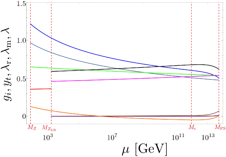
Figure 3: The running of various couplings. The red, green, blue, violet, black, aqua, purple, dark brown and orange lines stand for the evolution of $g_{\rm Y}$, $g_{2}$, $g_{3}$, $g_{\rm R}$, $g_{\rm B-L}$, $y_{t}$, $\lambda_{\rm r}$, $\lambda_{\rm m}$ and $\lambda$, respectively.

The values of $\lambda_{\rm r}$ and $\lambda_{\rm m}$ at $v_{\rm R}$ are estimated using stationary conditions (3.22) and $\lambda(v_{\rm R})$ with $\langle\varphi\rangle\approx 246$ GeV. Here, contributions from Kaluza-Klein modes of gauge bosons are added, but those from Kaluza-Klein modes of scalar fields are not considered because they are negligible small when $\lambda_{\rm r}$, $\lambda_{\rm m}$ and $\lambda$ take tiny values. The running of $\lambda$ is almost same as that in the SM because contributions from gluon and top quark are dominant. From Figure 3, we find that the vacuum stability is recovered by the rapid increase of $\lambda$ due to contributions from Kaluza-Klein modes of gauge bosons. We suppose that the vacuum stability problem could be solved by changing the running of $\lambda$ if $M_{\rm c}$ is less than $10^{7}$ GeV. But, in this case, $\lambda$ can generally blow up infinity much less than $M_{\rm PS}$ due to the threshold corrections of various Kaluza-Klein modes.

4 Conclusions and discussions

We have studied the origin of electroweak symmetry under the assumption that $SU(4)_{\rm C}\times SU(2)_{\rm L}\times SU(2)_{\rm R}$ is realized on the 5D space-time $M^{4}\times S^{1}/Z_{2}$. The Pati-Salam type gauge symmetry is reduced to $SU(3)_{\rm C}\times SU(2)_{\rm L}\times U(1)_{\rm R}\times U(1)_{\rm B-L}$ at a high-energy scale $M_{\rm PS}$ above the compactification scale $M_{\rm c}$ by orbifold breaking mechanism on $S^{1}/Z_{2}$. The breakdown of residual gauge symmetries occurs radiatively via the Coleman-Weinberg mechanism, such that the $U(1)_{\rm R}\times U(1)_{\rm B-L}$ symmetry is broken down to $U(1)_{\rm Y}$ by the VEV of an $SU(2)_{\rm L}$ singlet scalar field and the $SU(2)_{\rm L}\times U(1)_{\rm Y}$ symmetry is broken down to the electric one $U(1)_{\rm EM}$ by the VEV of the Higgs doublet, using the negative squared mass originated from an interaction between the Higgs doublet and an $SU(2)_{\rm L}$ singlet scalar field as a Higgs portal. The vacuum stability can be recovered by the contributions from Kaluza-Klein modes appearing at $M_{\rm c}$ and above there.

Our 3211 model has an excellent feature that $M_{\rm PS}$ is almost determined as $M_{\rm PS}=O(10^{13})$ GeV from the gauge coupling unification of $SU(3)_{\rm C}$ and $U(1)_{\rm B-L}$ into $SU(4)_{\rm C}$ and the left-right symmetry between $SU(2)_{\rm L}$ and $SU(2)_{\rm R}$. On the contrary, the breaking scale $v_{\rm R}$ of $U(1)_{\rm R}\times U(1)_{\rm B-L}$ is not fixed from the information of gauge couplings alone. The criterion of naturalness can favor $v_{\rm R}$ close to the weak scale.

Our 3211 model has almost same particle contents as those in a minimal $B-L$ extension of the SM proposed in [26, 27, 28, 29]. Main differences of our model and the $B-L$ extended SM are $U_{\rm B-L}$ charge assignment of $SU(2)_{\rm L}$ singlet scalar field $\phi_{\rm R}$ and the interactions between $U(1)$ gauge bosons and matter fields. In our model, the $\nu_{{\rm R}A}$ and $\phi_{\rm R}$ have $U(1)_{\rm B-L}$ charge of $-1/2$ and $1/2$, respectively. Then, allowed interaction terms between them are not renormalizable ones but non-renormalizable ones, e.g., $(f_{AB}/\Lambda)\phi_{\rm R}^{2}\overline{\nu}^{c}_{{\rm R}A}\nu_{{\rm R}A}$, where $\Lambda$ is a high-energy scale such as $M_{\rm PS}$. Hence small Majorana masses appear after the breakdown of $U(1)_{\rm R}\times U(1)_{\rm B-L}$ and the seesaw mechanism does not work at the TeV scale. In this paper, we focus on physics of gauge symmetry breaking sector. It would be meaningful to investigate flavor physics relating to quarks and leptons in our model. It would be also important to clarify the relationship between our model and the $B-L$ extended SM through the study of gauge kinetic mixing and so on.

References

- [1] ATLAS Collaboration, Phys. Lett. B 716, 1 (2012).
- [2] CMS Collaboration, Phys. Lett. B 716, 30 (2012).
- [3] J. C. Pati and A. Salam, Phys. Rev. D 10, 275 (1974).
- [4] L. Dixon, J. A. Harvey, C. Vafa and E. Witten, Nucl. Phys. B261, 678 (1985).
- [5] L. Dixon, J. A. Harvey, C. Vafa and E. Witten, Nucl. Phys. B274, 285 (1986).
- [6] L. Antoniadis, Phys. Lett. B246, 377 (1990).
- [7] P. Hořava and E. Witten, Nucl. Phys. B460, 506 (1996).
- [8] P. Hořava and E. Witten, Nucl. Phys. B475, 94 (1996).
- [9] E. A. Mirabelli and M. Peskin, Phys. Rev. D58, 065002 (1998).
- [10] A. Pomarol and M. Quriós, Phys. Lett. B438, 255 (1998).
- [11] J. Scherk and J. H. Schwarz, Phys. Lett. B82, 60 (1979).
- [12] J. Scherk and J. H. Schwarz, Nucl. Phys. B153, 61 (1979).
- [13] Y. Kawamura, Prog. Theor. Phys. 103, 613 (2000).
- [14] Y. Kawamura, Prog. Theor. Phys. 105, 999 (2001).
- [15] Y. Mimura and S. Nandi, Phys. Lett. B 538, 406 (2002).
- [16] R. N. Mohapatra and A. Pérez-Lorenzana, Phys. Rev. D 66, 035005 (2002).
- [17] S. Coleman and E. Weinberg, Phys. Rev. D 7, 1888 (1973).
- [18] G. Senjanovic and R. N. Mohapatra, Phys. Rev. D 12, 1502 (1975).
- [19] M. Cvetič, Nucl. Phys. B 233, 387 (1984).
- [20] M. Holthausen, M. Lindner and M. A. Schmidt, Phys. Rev. D 82, 055002 (2010).
- [21] P. S. Bhupal Dev, R. N. Mohapatra and Y. Zhang, arXiv:1703.02471.
- [22] R. Hempfling, Phys. Lett. B 379, 153 (1996).
- [23] K. R. Dienes, E. Dudas and T. Gherghetta, Phys. Lett. B 436, 55 (1998).
- [24] K. R. Dienes, E. Dudas and T. Gherghetta, Nucl. Phys. B 537, 47 (1999).
- [25] C. Patrignani et al. (Particle Date Group), Chin. Phys. C 40, 100001 (2016) and 2017 update (http://pdg.lbl.gov/).
- [26] S. Khalil, J. Phys. G 35, 055001 (2008).
- [27] S. Iso, N. Okada and Y. Orikasa, Phys. Lett. B 676, 81 (2009).
- [28] S. Iso, N. Okada and Y. Orikasa, Phys. Rev. D 80, 115007 (2009).
- [29] S. Iso and Y. Orikasa, Prog. Theor. Exp. Phys. 2013, 023B08 (2013).