Explaining hyperspectral imaging based plant disease identification: 3D CNN and saliency maps

Abstract

Our overarching goal is to develop an accurate and explainable model for plant disease identification using hyperspectral data. Charcoal rot is a soil borne fungal disease that affects the yield of soybean crops worldwide. Hyperspectral images were captured at 240 different wavelengths in the range of 383 - 1032 nm. We developed a 3D Convolutional Neural Network model for soybean charcoal rot disease identification. Our model has classification accuracy of 95.73$\%$ and an infected class F1 score of 0.87. We infer the trained model using saliency map and visualize the most sensitive pixel locations that enable classification. The sensitivity of individual wavelengths for classification was also determined using the saliency map visualization. We identify the most sensitive wavelength as 733 nm using the saliency map visualization. Since the most sensitive wavelength is in the Near Infrared Region (700 - 1000 nm) of the electromagnetic spectrum, which is also the commonly used spectrum region for determining the vegetation health of the plant, we were more confident in the predictions using our model.

1 Introduction

Deep Convolutional Neural Networks(CNN) have led to rapid developments in diverse applications such as object recognition, speech recognition, document reading and sentiment analysis within the industry and social media (Krizhevsky et al., 2012b; Waibel et al., 1989; LeCun et al., 1998; Dos Santos and Gatti, 2014). Recently, 3D-CNN models have been used in classification of hyperspectral images for different objects of interest (Fotiadou et al., 2017; Chen et al., 2016; Li et al., 2017). But now that we are trying to leverage CNN’s for science applications, where simply prediction results will not be sufficient to trust the decision making of our model (Lipton, 2016). Therefore, we need interpretability methods for visualizing the information learnt by the model. There are many emerging techniques for interpreting CNN Montavon et al. (2017) and one of them is saliency map based visualization developed by (Simonyan et al., 2013). Here we show, an important science application of it in the domain of plant pathology.

Plant diseases negatively impact yield potential of crops worldwide, including soybean [Glycine max (L.) Merr.], reducing the average annual soybean yield by an estimated 11% in the United States (Hartman et al., 2015). However, today’s disease scouting and phenotyping techniques predominantly rely on human scouts and visual ratings. Human visual ratings are dependent on rater ability, rater reliability, and can be prone to human error, subjectivity, and inter/intra-rater variation (Bock et al., 2010). So there is a need for improved technologies for disease detection and identification beyond visual ratings in order to improve yield protection.

Charcoal rot is an important fungal disease for producers in the United States and Canada, ranking among the top 7 most severe diseases in soybean from 2006 - 2014 and as high as the 2nd most yield limiting soybean disease in 2012 (Allen et al., 2017; Koenning et al., 2010). Charcoal rot has a large host range affecting other important economic crops such as corn, cotton, and sorghum making crop rotation a difficult management strategy (Short et al., 1980; Su et al., 2001). However, both field scouting for disease detection and small scale methods of charcoal rot evaluation still rely on visual ratings. These field and greenhouse screening methods for charcoal rot are time consuming and labor intensive.

Unlike visual ratings which only utilize visible(400-700 nm) region wavelengths, hyperspectral imaging can capture spectral and spatial information from wavelengths beyond human vision offering more usable information for disease detection. Hyperspectral imaging has been used for the detection and identification of plant diseases in barley, sugar beet, and wheat among others (Bauriegel et al., 2011; Kuska et al., 2015; Mahlein et al., 2010). In addition, hyperspectral imaging offers a potential solution to the scalability and repeatability issues faced with human visual ratings. Because of large data dimensions and redundancy, machine learning based methods are well suited to convert hyperspectral data into actionable information (Singh et al., 2016).

In this work, we develop a supervised 3D-CNN based model to learn the spectral and spatial information of hyperspectral images for classification of healthy and charcoal rot infected samples. A saliency map based visualization method is used to identify the hyperspectral wavelengths that are most sensitive for the classification. We infer the importance of the wavelengths by analyzing the magnitude of saliency map gradient distribution of the image across the hyperspectral wavelengths. To the best of our knowledge, this is the first work done on exploring the interpretation for the classification of hyperspectral data using saliency maps. This work is a societally relevant example of utilizing saliency maps to enable explanations of cues from hyperspectral data for disease identification. We are much more confident in the predictions of the model due to the physiologically meaningful explanations from the saliency visualization.

2 Experiments

2.1 Dataset

Healthy and infected soybean stem samples were collected at 3, 6, 9, 12, and 15 days after charcoal rot infection. Hyperspectral data cubes of the exterior of the infected and healthy stems were captured at each time point of data collection prior to disease progression length measurements. The hyperspectral imaging system consisted of a Pika XC hyperspectral line imaging scanner, including the imager mounted on a stand, a translational stage, a laptop with SpectrononPro software for operating the imager and translational stage during image collection (Resonon, Bozeman, MT), and two 70-watt quartz-tungsten-halogen Illuminator lamps (ASD Inc., Boulder, CO) to provide stable illumination over a 400 – 1000 nm range. The Pika XC Imager collects 240 wavebands over a spectral range from 400 – 1000 nm with a 2.5 nm spectral resolution. The hyperspectral camera setup used in this study is shown in Figure 1a. Figure 1b shows an example of soybean stem captured at different hyperspectral wavelengths. The disease spread length from top of the stem is available for all the infected stem images which were used the for ground truth labeling of image classes. A reddish-brown lesion was developed on the stem due to charcoal rot infection often progressing farther down the inside of the stem than visible on the exterior of the stem. Figure 1c shows the RGB image of the disease progression comparison between interior and exterior region of a soybean stem. The data-set contains 111 hyperspectral stem images of size 500x1600x240. Among the 111 images, 64 represent healthy stems and 47 represent infected stems. Data patches of resolution 64x64x240 pixels were extracted from the stem images. The 64x64x240 image patches were applied as input to the 3D-CNN model. The training dataset consists of 1090 images. Out of 1090 training images, 940 images represent healthy stem and 150 images represent infected stem. All the images were normalized between 0 and 1. The validation and test dataset consists of 194 and 539 samples respectively.

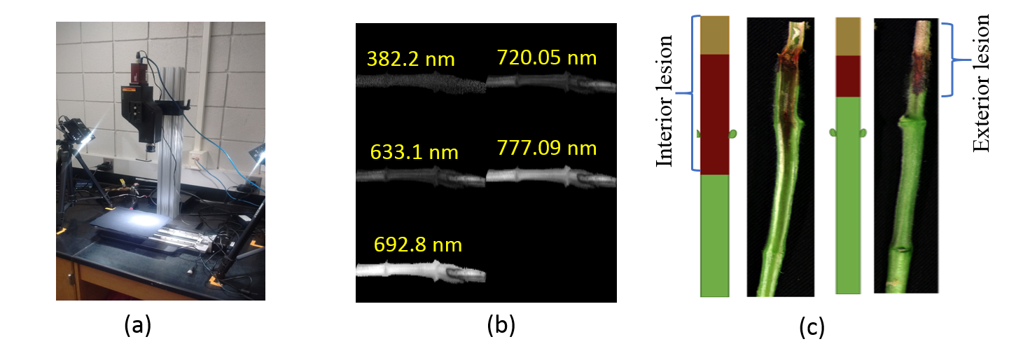
Figure 1: (a) Hyperspectral camera setup used in this study. (b) An example of a soybean stem imaged at different hyperspectral wavelengths. (c) RGB image of the disease progression comparison between interior and exterior region of soybean stem. Soybean stem was sliced in half , interior lesion length and exterior lesion length were measured in mm.

2.2 Model Architecture

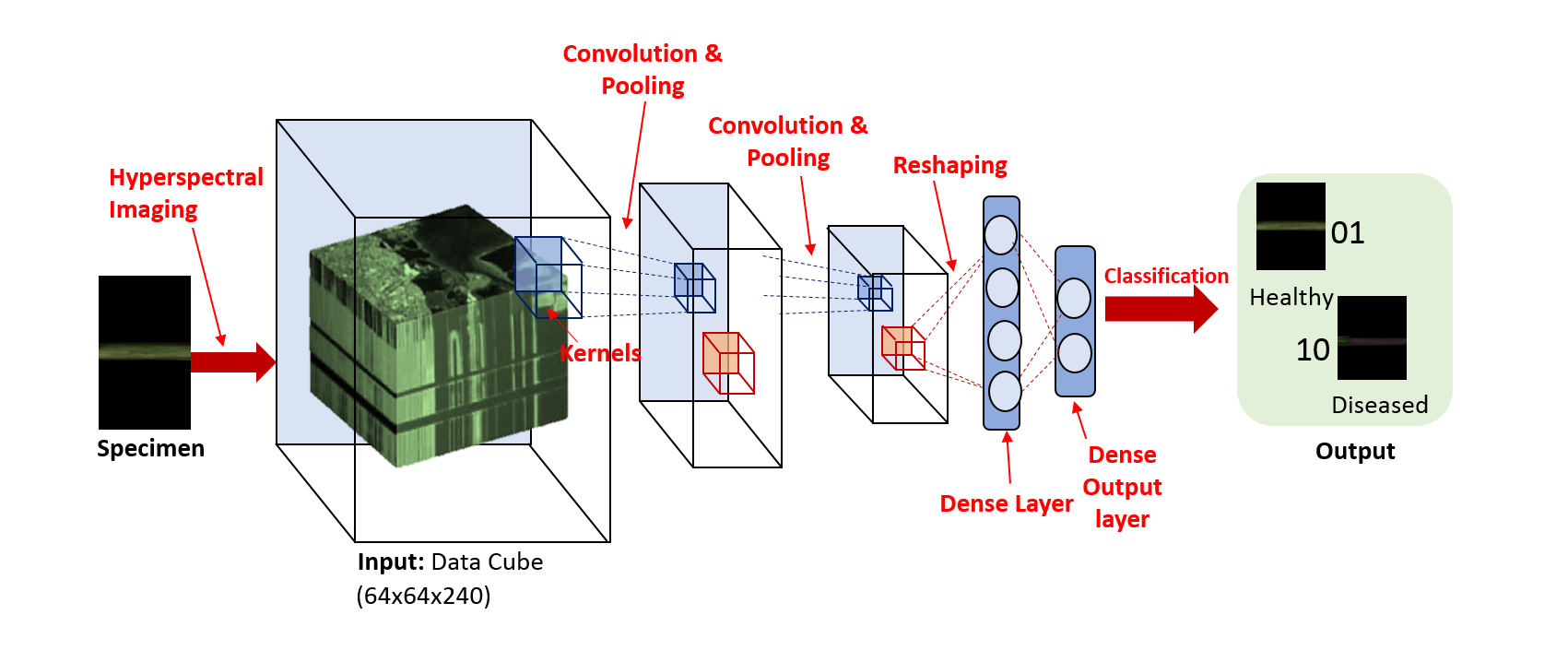
Figure 2: 3D Convolutional Neural Network Architecture for Classification.

The 3D-CNN model consists of 2 convolutional layers interspersed with 2 max pooling layers followed by 2 fully connected layers. A relatively small architecture was used to prevent overfitting during training. Two kernels of size 3x3x16 (3x3 in spatial dimension and 16 in spectral dimension) were used for convolving the input of the first convolution layer and four kernels of size 3x3x16 were used in the second convolution layer. Rectified Linear Input(RELU) was used as the activation function for the convolution output (Glorot et al., 2011). A 2x2x2 maxpooling was applied on the output of each convolutional layer. Dropout with a probability of 0.25 was performed after first max pooling operation and with a probability of 0.5 after the first fully-connected layer. Dropout mechanism was used to prevent overfitting during training (Krizhevsky et al., 2012a). The first fully-connected layer consists of 16 nodes. The output of the second fully-connected layer (2 nodes) is fed to a softmax layer. Figure-2 summarizes the 3D convolutional neural network architecture used in the study.

2.3 Training

Adam optimizer was used to train our convolutional network weights on mini-batches of size 32 (Kingma and Ba, 2014). We use a learning rate value $1$ x $10^{-}6$ and set $\beta_{1}$=0.9, $\beta_{2}$=0.999 and $\epsilon$ = $10^{-8}$. The convolution layer kernels were initialized with normal distribution with standard deviation of 0.05 and biases were initialized with zero. The dense layer neurons were initialized using glorot initialization (Glorot and Bengio, 2010). The 3D-CNN model was trained for 126 epochs. Here, we use all the 240 wavelength bands of hyperspectral images for classification purpose. We trained using Keras (Chollet et al., 2015) with Tensorflow (Abadi et al., 2015) backend on a NVIDIA Tesla P40 GPU.

2.4 Class Balanced Loss Function

Because of imbalanced training data, weighted binary cross-entropy was used as a loss function. The loss ratio was 1:6.26 between more frequent healthy class samples and less frequent infected class samples. The class balanced loss improved our classification accuracy and F1-score.

2.5 Classification Results

We evaluate the learned 3D-CNN model on 539 test images. Table 1 shows the classification results of the 3D CNN model. Classification accuracy of 95.73% and precision value of 0.92 indicates a good generalizing capacity of the model for different infected stages of disease. The recall score is lower compared to precision score as disease severity indications are very sparse in some locations of the exterior stem region. The F1-score of infected class of the test data was 0.87.

Table 1: Classification Results

Precision	Recall	F1-Score	Classification Accuracy
0.92	0.82	0.87	95.73

2.6 Saliency Map Visualization

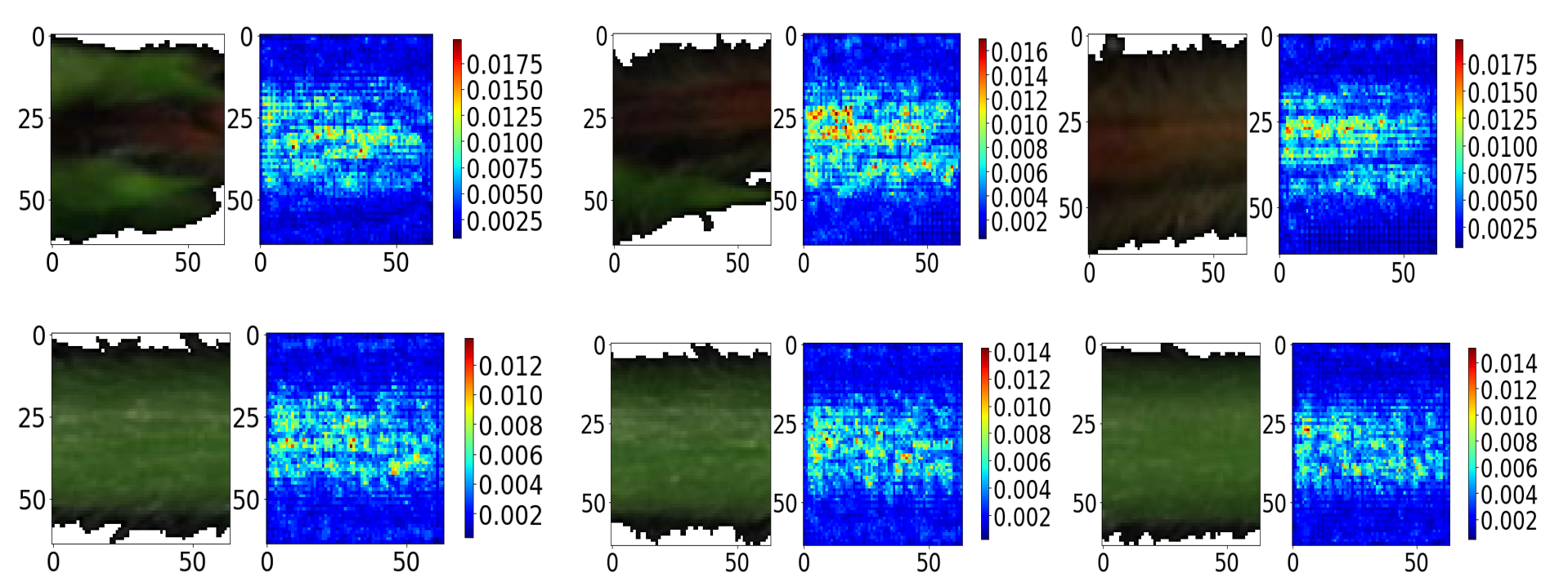
Figure 3: Image specific class saliency maps for the infected(Top) and healthy(Bottom) test images. The magnitude of the gradient of the maximum predicted class score with respect to the input image in the visualizations illustrate the sensitivity of the pixels to classification.

We visualize the parts of the image that were most sensitive to the classification using image specific class saliency map. Specifically, the magnitude of the gradient of the maximum predicted class score with respect to the input image was used to identify the most sensitive pixel locations for classification (Simonyan et al., 2013). The saliency map visualizations of the healthy and infected samples are shown in Figure 3. The magnitude of gradient of each pixel indicates the relative importance of the pixel in the prediction of the output class score. The saliency maps of the infected stem images has high magnitude of gradient values in locations corresponding to the severely infected regions(reddish-brown) of the image as shown in the Figure 3. This indicates that the severely infected regions of the image contains the most sensitive pixel locations for prediction of the infected class score. For both the healthy and infected images, the saliency map gradients were concentrated around the mid region of the stem.

2.7 Explaining importance of hyperspectral wavelengths for classification using saliency maps

Let $I_{1},I_{2},...I_{N}$ be the $N$ test images for disease classification. Let $W$ be the gradient of the maximum predicted class score with respect to the input image. Each pixel $(x,y)$ in the image $I_{i}$ is maximally activated by one of the 240 wavelength channels. Let us assume that the element index of $W$ corresponding to a pixel location $(x,y)$ in wavelength channel $C$ of a image $I_{i}$ is $g(x,y,C)$. For each pixel location $(x,y)$ in image $I_{i}$, let $C^{\textbf{*}}$ be the wavelength with maximum magnitude of $W$ across all channels.

$$C^{\textbf{*}}=\operatorname*{argmax}_{C{\in}{(1,2,...240)}}|W_{g(x,y,C)}|\;\textbf{For}\;(x,y)\in I_{i}$$ (1)

Note, that $C^{\textbf{*}}$ is a function of $(x,y)$. The histogram of $C^{\textbf{*}}$ from all pixel locations of the $N$ test images is shown in Figure 4. It illustrates the percentage of pixel locations from all $N$ test images with maximum saliency gradient magnitude from each wavelength. The importance of a specific hyperspectral wavelength can be quantified by the percentage of pixels with maximum saliency gradient magnitude in that wavelength. The histogram reveals several important aspects of our model. First, wavelength 733 nm ($C^{\textbf{*}}$=130) from the near-infrared region was the most sensitive among all wavelengths in the test data. Second, the 15 wavelengths in the spectral region of 703 to 744 nm were responsible for maximum magnitude of gradient values in 33% of the pixel locations of the test image. Further, the wavelengths in the visible region of the spectrum (400-700 nm) were more sensitive for the infected samples compared to the healthy samples.

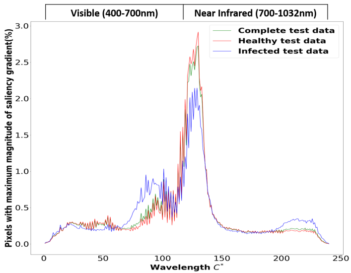
Figure 4: Histogram of $C^{\textbf{*}}$ from all the test images. It illustrates the percentage of pixel locations from all $N$ test images with maximum magnitude of saliency gradient from each wavelength.

The magnitude of the gradient of maximum predicted class score with respect to the the most sensitive wavelength channel $C^{\textbf{*}}=130$ (733 nm) of the test data is shown in Figure 5. Wavelength specific data gradient magnitude reveals the sensitivity of pixels in that wavelength for classification. Hence, wavelength specific visualization is helpful in understanding the importance of a individual wavelengths for classification.

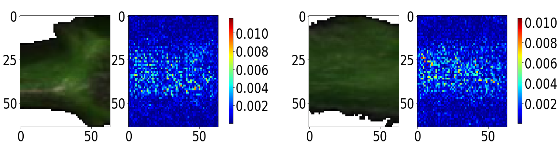
Figure 5: Visualizations illustrate the magnitude of the gradient of the maximum predicted class score with respect to the most sensitive wavelength $C^{\textbf{*}}=130$ (733 nm) of the complete test data. $C^{\textbf{*}}=130$ is the wavelength which has maximum saliency gradient magnitude at most number of pixel locations in the complete test data.

3 Conclusions

We have demonstrated that a 3D CNN model can effectively be used to learn the high dimensional hyperspectral data to identify charcoal rot disease in soybeans. We show that a saliency map visualization can be used to explain the importance of hyperspectral wavelengths in classification. Thus, using saliency map enabled interpretability, the model was able to track the physiological insights of the predictions. Hence, we are more confident of the predictive capability of our model. In future, band selection based on robust interpretability mechanisms will be helpful in dimensionality reduction of the large hyperspectral data and also in designing a multispectral camera system for high throughput phenotyping.

References

- Abadi et al. [2015] Martín Abadi, Ashish Agarwal, Paul Barham, Eugene Brevdo, Zhifeng Chen, Craig Citro, Greg S. Corrado, Andy Davis, Jeffrey Dean, Matthieu Devin, Sanjay Ghemawat, Ian Goodfellow, Andrew Harp, Geoffrey Irving, Michael Isard, Yangqing Jia, Rafal Jozefowicz, Lukasz Kaiser, Manjunath Kudlur, Josh Levenberg, Dan Mané, Rajat Monga, Sherry Moore, Derek Murray, Chris Olah, Mike Schuster, Jonathon Shlens, Benoit Steiner, Ilya Sutskever, Kunal Talwar, Paul Tucker, Vincent Vanhoucke, Vijay Vasudevan, Fernanda Viégas, Oriol Vinyals, Pete Warden, Martin Wattenberg, Martin Wicke, Yuan Yu, and Xiaoqiang Zheng. TensorFlow: Large-scale machine learning on heterogeneous systems, 2015. URL https://www.tensorflow.org/. Software available from tensorflow.org.
- Allen et al. [2017] T W Allen, C A Bradley, A J Sisson, E Byamukama, M I Chilvers, C M Coker, A A Collins, J P Damicone, A E Dorrance, and N S Dufault. Soybean yield loss estimates due to diseases in the United States and Ontario, Canada, from 2010 to 2014. Plant Health Prog, 18:19–27, 2017.
- Bauriegel et al. [2011] E Bauriegel, A Giebel, M Geyer, U Schmidt, and W B Herppich. Early detection of Fusarium infection in wheat using hyper- spectral imaging. Computers and Electronics in Agriculture, 75(2):304–312, 2011. ISSN 0168-1699. doi: 10.1016/j.compag.2010.12.006.
- Bock et al. [2010] C. H. Bock, G. H. Poole, P. E. Parker, and T. R. Gottwald. Plant disease severity estimated visually, by digital photography and image analysis, and by hyperspectral imaging. Critical Reviews in Plant Sciences, 29(2):59–107, 2010. ISSN 07352689. doi: 10.1080/07352681003617285.
- Chen et al. [2016] Yushi Chen, Hanlu Jiang, Chunyang Li, Xiuping Jia, and Senior Member. Deep feature extraction and classification of hyperspectral images based on Convolutional Neural Networks. IEE Transactions on Geoscience and Remote Sensing, 54(10):6232–6251, 2016. doi: 10.1109/TGRS.2016.2584107.
- Chollet et al. [2015] François Chollet et al. Keras. https://github.com/fchollet/keras, 2015.
- Dos Santos and Gatti [2014] Cícero Nogueira Dos Santos and Maira Gatti. Deep convolutional neural networks for sentiment analysis of short texts. In COLING, pages 69–78, 2014.
- Fotiadou et al. [2017] Konstantina Fotiadou, Grigorios Tsagkatakis, and Panagiotis Tsakalides. Deep convolutional neural networks for the classification of snapshot mosaic hyperspectral imagery. Electronic Imaging, 2017(17):185–190, 2017.
- Glorot and Bengio [2010] Xavier Glorot and Yoshua Bengio. Understanding the difficulty of training deep feedforward neural networks. In Yee Whye Teh and Mike Titterington, editors, Proceedings of the Thirteenth International Conference on Artificial Intelligence and Statistics, volume 9 of Proceedings of Machine Learning Research, pages 249–256, Chia Laguna Resort, Sardinia, Italy, 13–15 May 2010. PMLR. URL http://proceedings.mlr.press/v9/glorot10a.html.
- Glorot et al. [2011] Xavier Glorot, Antoine Bordes, and Yoshua Bengio. Deep sparse rectifier neural networks. In Proceedings of the Fourteenth International Conference on Artificial Intelligence and Statistics, pages 315–323, 2011.
- Hartman et al. [2015] Glen Lee Hartman, John Clark Rupe, Edward J Sikora, Leslie Leigh Domier, Jeff A Davis, and Kevin Lloyd Steffey. Compendium of soybean diseases and pests. Am Phytopath Society, 2015.
- Kingma and Ba [2014] Diederik Kingma and Jimmy Ba. Adam: A method for stochastic optimization. arXiv preprint arXiv:1412.6980, 2014.
- Koenning et al. [2010] Stephen R Koenning, J Allen Wrather, et al. Suppression of soybean yield potential in the continental united states by plant diseases from 2006 to 2009. Plant Health Progress, 10, 2010.
- Krizhevsky et al. [2012a] Alex Krizhevsky, Ilya Sutskever, and Hinton Geoffrey E. ImageNet Classification with Deep Convolutional Neural Networks. Advances in Neural Information Processing Systems 25 (NIPS2012), pages 1–9, 2012a. ISSN 10495258. doi: 10.1109/5.726791. URL https://papers.nips.cc/paper/4824-imagenet-classification-with-deep-convolutional-neural-networks.pdf.
- Krizhevsky et al. [2012b] Alex Krizhevsky, Ilya Sutskever, and Geoffrey E Hinton. Imagenet classification with deep convolutional neural networks. In Advances in neural information processing systems, pages 1097–1105, 2012b.
- Kuska et al. [2015] Matheus Kuska, Mirwaes Wahabzada, Marlene Leucker, Heinz-Wilhelm Dehne, Kristian Kersting, Erich-Christian Oerke, Ulrike Steiner, and Anne-Katrin Mahlein. Hyperspectral phenotyping on the microscopic scale: towards automated characterization of plant-pathogen interactions. Plant Methods, 11(1):28, 2015. ISSN 1746-4811. doi: 10.1186/s13007-015-0073-7. URL http://www.plantmethods.com/content/11/1/28.
- LeCun et al. [1998] Yann LeCun, Léon Bottou, Yoshua Bengio, and Patrick Haffner. Gradient-based learning applied to document recognition. Proceedings of the IEEE, 86(11):2278–2324, 1998.
- Li et al. [2017] Ying Li, Haokui Zhang, and Qiang Shen. Spectral–Spatial Classification of Hyperspectral Imagery with 3D Convolutional Neural Network. Remote Sensing, 9(1):67, 2017. ISSN 2072-4292. doi: 10.3390/rs9010067. URL http://www.mdpi.com/2072-4292/9/1/67.
- Lipton [2016] Zachary C Lipton. The mythos of model interpretability. arXiv preprint arXiv:1606.03490, 2016.
- Mahlein et al. [2010] A. K. Mahlein, U. Steiner, H. W. Dehne, and E. C. Oerke. Spectral signatures of sugar beet leaves for the detection and differentiation of diseases. Precision Agriculture, 11(4):413–431, 2010. ISSN 13852256. doi: 10.1007/s11119-010-9180-7.
- Montavon et al. [2017] Grégoire Montavon, Wojciech Samek, and Klaus-Robert Müller. Methods for interpreting and understanding deep neural networks. Digital Signal Processing, 2017.
- Short et al. [1980] GE Short, TD Wyllie, and PR Bristow. Survival of macrophomina phaseolina in soil and in residue of soybean. Survival, 7(13):17, 1980.
- Simonyan et al. [2013] Karen Simonyan, Andrea Vedaldi, and Andrew Zisserman. Deep inside convolutional networks: Visualising image classification models and saliency maps. arXiv preprint arXiv:1312.6034, 2013.
- Singh et al. [2016] Arti Singh, Baskar Ganapathysubramanian, Asheesh Kumar Singh, and Soumik Sarkar. Machine learning for high-throughput stress phenotyping in plants. Trends in plant science, 21(2):110–124, 2016.
- Su et al. [2001] G. Su, S.-O. Suh, R. W. Schneider, and J. S. Russin. Host Specialization in the Charcoal Rot Fungus, <i>Macrophomina phaseolina</i>. Phytopathology, 91(2):120–126, 2001. ISSN 0031-949X. doi: 10.1094/PHYTO.2001.91.2.120. URL http://apsjournals.apsnet.org/doi/10.1094/PHYTO.2001.91.2.120.
- Waibel et al. [1989] Alex Waibel, Toshiyuki Hanazawa, Geoffrey Hinton, Kiyohiro Shikano, and Kevin J Lang. Phoneme recognition using time-delay neural networks. IEEE transactions on acoustics, speech, and signal processing, 37(3):328–339, 1989.