Spectral Approximation of Convolution Operator

Abstract

We develop a unified framework for constructing matrix approximations to the convolution operator of Volterra type defined by functions that are approximated using classical orthogonal polynomials on $[-1,1]$. The numerically stable algorithms we propose exploit recurrence relations and symmetric properties satisfied by the entries of these convolution matrices. Laguerre-based convolution matrices that approximate Volterra convolution operator defined by functions on $[0,\infty]$ are also discussed for the sake of completeness.

1 Introduction

Convolution operators abound in science and engineering. They can be found in, for example, statistics and probability theory [15], computer vision [11], image and signal processing [5], and system control [22]. In applied mathematics, convolution operators figure in many topics, from Green’s function [9] to Duhamel’s principle [23], from non-reflecting boundary condition [12] to large eddy simulation [27], from approximation theory [26] to fractional calculus [14]. Furthermore, convolution operators are the key building blocks of the convolution integral equations [1, 17, 4].

Given two continuous functions $f(x)$ and $g(x)$ on the interval $[-1,1]$, the (left-sided) convolution operator $V$ of Volterra type defined by $f(x)$ is given by

(1) $$V[f](g)=h(x)=\int_{-1}^{x+1}f(x-t)g(t)\mathrm{d}t,~{}~{}~{}~{}~{}x\in[-2,0].$$

For more general cases where $f(x):[a,b]\to\mathbb{R}$ and $g(x):[c,d]\to\mathbb{R}$ with $b-a=d-c$, the convolution operator can be shown equivalent to (1) via changes of variables and rescaling. Thus we only consider (1) throughout without loss of generality.

If $f(x)$ and $g(x)$ have a little extra smoothness beyond continuity, they can be approximated by polynomials $f_{M}(x)$ and $g_{N}(x)$ of sufficiently high degree so that $\|f(x)-f_{M}(x)\|_{\infty}$ and $\|g(x)-g_{N}(x)\|_{\infty}$ are on the order of machine precision [26, 8]. In this article, we focus on the approximation of $V[f]$ when $f(x)$ and $g(x)$ are approximated using the orthogonal polynomials of the Jacobi family, e.g. the Chebyshev polynomials:

(2) $$f_{M}(x)=\sum_{m=0}^{M}a_{m}T_{m}(x)~{}~{}~{}\mbox{and}~{}~{}~{}g_{N}(x)=\sum_{n=0}^{N}b_{n}T_{n}(x),$$

where $T_{m}(x)=\cos(m\arccos x)$ for $x\in[-1,1]$ is the $m$-th Chebyshev polynomial.

This way, the polynomial approximant $h_{M+N+1}(x)$ of the convolution $h(x)$ can be written as the product of a $[-2,0]\times(N+1)$ column quasi-matrix $\widetilde{R}$ and the coefficient vector $\underline{b}=(b_{0},\ldots,b_{N})^{T}$

(3) $$h_{M+N+1}(x)=\widetilde{R}\underline{b}=\begin{bmatrix}[c|c|c|c]&&&\\ &&&\\ (f_{M}{\ast}T_{0})(x)&(f_{M}{\ast}T_{1})(x)&\cdots&(f_{M}{\ast}T_{N})(x)\\ &&&\\ &&&\end{bmatrix}\underline{b},$$

where the $n$-th column of $\widetilde{R}$ is the convolution of $f_{M}(x)$ and $T_{n}(x)$. Besides the notation we have introduced, asterisks are also used here and in the remainder of this paper to denote the convolution of two functions. For example, $(f_{M}\ast T_{n})(x)$ is the convolution of $f_{M}(x)$ and $T_{n}(x)$. For convenience, we will also denote by $\widetilde{R}_{n}$ the $n$-th column of $\widetilde{R}$, i.e. $(f_{M}\ast T_{n})(x)$, with the index $n$ starting from $0$.

If $h_{M+N+1}(x)$ and $\{(f_{M}\ast T_{n})(x)\}_{n=0}^{N}$ are translated to $[-1,1]$ by the change of variables $y=x+1$, they can be expressed as Chebyshev series of degree $M+N+1$ and $M+n+1$, respectively:

(4) $$\begin{array}[]{l l}\begin{aligned} h_{M+N+1}(y)&=\sum_{k=0}^{M+N+1}c_{k}T_{k}(y),\\ (f_{M}\ast T_{n})(y)&=\sum_{k=0}^{M+N+1}R_{k,n}T_{k}(y),~{}~{}~{}~{}0\leqslant n\leqslant N,\end{aligned}\end{array}$$

where $y\in[-1,1]$ and $R_{k,n}=0$ for any $k>M+n+1$. Substituting (4) into (3), we have

(5) $$\sum_{k=0}^{M+N+1}c_{k}T_{k}(y)=\sum_{n=0}^{N}b_{n}\sum_{k=0}^{M+N+1}R_{k,n}T_{k}(y),$$

or, equivalently,

(6) $$\underline{c}=R\underline{b},$$

where $\underline{c}=(c_{0},\ldots,c_{M+N+1})^{T}$ and $R$ is an $(M+N+2)\times(N+1)$ matrix that collects the Chebyshev coefficients of $\widetilde{R}_{n}$ for $0\leqslant n\leqslant N$. Since $R_{k,n}=0$ for $k>M+n+1$, the lower triangular part of $R$ below $(M+1)$-th subdiagonal are zeros (see Figure 1). We shall call $R$ the convolution matrix that approximates the convolution operator $V[f]$. What makes $R$ important is the fact that with $R$ available either of $\underline{b}$ and $\underline{c}$ can be calculated when the other is given. Thus our goal is to calculate $R$ accurately and efficiently.

Thus far the only attempt to approximate the convolution operator in the same vein was given by Hale and Townsend [13], where they considered the same problem but with $f(x)$ and $g(x)$ approximated by Legendre series. Their method exploits the fact that the Fourier transform of Legendre polynomial $P_{m}(x)$ is spherical Bessel function $j_{m}(x)$ with a simple rescaling. They also show that $(P_{m}\ast P_{n})(x)$ can be represented as a rescaled inverse Fourier transform of the product $j_{m}(x)j_{n}(x)$, due to the convolution theorem. Based on these results, the entries of a Legendre-based convolution matrix $R^{(1/2)}$ are represented as infinite integrals involving triple-product of spherical Bessel functions and the three-term recurrence satisfied by spherical Bessel functions finally leads to a four-term recurrence relation satisfied by the entries of $R^{(1/2)}$. Unfortunately, the Fourier transforms of other classical orthogonal polynomials do not have a simple representation in terms of spherical Bessel functions or other special functions that enjoy a similar recurrence relation [6]. Therefore, the method in [13] cannot be easily extended to the cases where $f(x)$ and $g(x)$ are approximated using other classical orthogonal polynomials, e.g. Chebyshev, and this is what this article addresses.

In another work with a similar setting [30], spectral approximations of convolution operators are constructed when $f(x)$ and $g(x)$ are approximated by Fourier extension approximants. It is shown that convolution can be represented in terms of products of Toeplitz matrices and coefficient vectors of the Fourier extension approximants, based on which an $\mathcal{O}(N^{\prime}(\log N^{\prime})^{2})$ fast algorithm is derived for approximating the convolution of compactly supported functions, where $N^{\prime}$ is the number of degrees of freedom in each of the Fourier extension approximants for $f(x)$ and $g(x)$.

In an investigation carried out simultaneously [18], closed-form formulae are derived for the convolution of classical orthogonal polynomials. However, this explicit formula is too complicated and numerically intractable to be computationally useful for direct construction of $R$.

In this article, we first generalize the recurrence relation found in [13] to Chebyshev-based convolution matrices. Instead of resorting to the Fourier transform of Chebyshev polynomials and recurrence of spherical Bessel functions, we exploit the three-term recurrence of the derivatives of Chebyshev polynomials to show a recurrence relation satisfied by the columns of $\widetilde{R}$. Further, a five-term recurrence relation satisfied by the entries of $R$ can be obtained by replacing columns of $\widetilde{R}$ with their Chebyshev coefficients. With this recurrence relation and a symmetric property, the entries of $R$ can be calculated efficiently and numerically stably, yielding spectral approximations to the convolution operators of Volterra type. The accuracy of $R$ and its applications are shown by various numerical examples. Finally, we extend our approach to broader Jacobi-family orthogonal polynomials, where the results of [13] are covered as a special case.

Our exposition could either begin with the Jacobi-based convolution and treat Gegenbauer, Legendre, and Chebyshev as special cases in a cascade, or start with Chebyshev, extend to Gegenbauer, and further to Jacobi. We choose the latter, since most derivations and proofs are much simpler with Chebyshev polynomials and analogues can be easily drawn to others. Also, the Chebyshev-based convolution is the most commonly-used in practice and, therefore, deserves a more elaborated discussion.

Our discussion is organized as follows. In Section 2, we derive the recurrence relation satisfied by columns of $\widetilde{R}$. In Section 3, the recurrence relation for entries of $R$ is derived based on that of $\widetilde{R}$. We show a stability issue when this recurrence relation is naively used for the construction of $R$ and provide a numerically stable algorithm by making use of the symmetric structure of $R$. In Section 4, we extend the results of Sections 2 and 3 to Gegenbauer- and Jacobi-based convolution matrices. The main results of this paper are complemented in Section 5 by a brief discussion about the approximation of the convolution operators defined by functions on $[0,\infty]$ using weighted Laguerre polynomials, before we give a few closing remarks in the final section.

2 Recurrence satisfied by convolutions of Chebyshev polynomials

We start with the following recurrence relation that can be derived from the fundamental three-term recurrence relation of Chebyshev polynomials.

Lemma 1.

For $n\geqslant 0$, the $n$-th Chebyshev polynomial $T_{n}(x)$ can be written as a combination of the derivatives of $T_{n-1}$ and $T_{n+1}$:

(7a) $$T_{n}(x)=\begin{cases}\displaystyle\frac{1}{2(n+1)}\frac{\mathrm{d}T_{n+1}(x)}{\mathrm{d}x}-\frac{1}{2(n-1)}\frac{\mathrm{d}T_{|n-1|}(x)}{\mathrm{d}x},&\quad n\neq 1,\\[11.38109pt] \displaystyle\frac{1}{4}\frac{\mathrm{d}T_{2}(x)}{\mathrm{d}x},&\quad n=1,\end{cases}$$

by integrating which we have the recurrence relation of Chebyshev polynomials and their indefinite integrals:

(7b) $$\int T_{n}(t)\mathrm{d}t=\begin{cases}\displaystyle\frac{T_{n+1}(x)}{2(n+1)}-\frac{T_{|n-1|}(x)}{2(n-1)},&\quad n\neq 1,\\[11.38109pt] \displaystyle T_{2}(x)/4,&\quad n=1.\end{cases}$$

Proof.

The proof can be found in many standard texts on Chebyshev polynomials. See, for example, [19, p. 32]. ∎

Like the convolution of functions defined on the entire real line, the convolution operator $V[f]$ also enjoys commutativity:

(8) $$\int_{-1}^{x+1}f(x-t)g(t)\mathrm{d}t=\int_{-1}^{x+1}f(t)g(x-t)\mathrm{d}t,~{}~{}~{}x\in[-2,0],$$

which can be shown by a change of variables with $T=x-t$.

Our first main result is the recurrence relation satisfied by the convolutions of a Chebyshev series and Chebyshev polynomials, which follows as a consequence of (7a).

Theorem 2 (Recurrence of convolutions of Chebyshev polynomials).

The convolutions of Chebyshev polynomials and the Chebyshev series $f_{M}(x)$ given in (2) recurse as follows:

(9a) $$\int_{-1}^{y}f_{M}(x-t)T_{0}(t)\mathrm{d}t=\int_{-1}^{y}f_{M}(t)\mathrm{d}t,$$

(9b) $$\int_{-1}^{y}f_{M}(x-t)T_{1}(t)\mathrm{d}t=\int_{-1}^{y}\int_{-1}^{x+1}f_{M}(t)\mathrm{d}t\,\mathrm{d}(x+1)-\int_{-1}^{y}f_{M}(t)\mathrm{d}t,$$

(9c) $$\int_{-1}^{y}f_{M}(x-t)T_{2}(t)\mathrm{d}t=4\int_{-1}^{y}\int_{-1}^{x+1}f_{M}(x-t)T_{1}(t)\mathrm{d}t\,\mathrm{d}(x+1)+\int_{-1}^{y}f_{M}(t)\mathrm{d}t,$$

and for $$n\geqslant 2$$,

(9d) $$\begin{multlined}\int_{-1}^{y}f_{M}(x-t)T_{n+1}(t)\mathrm{d}t=2(n+1)\int_{-1}^{y}\int_{-1}^{x+1}f_{M}(x-t)T_{n}(t)\mathrm{d}t\,\mathrm{d}(x+1)\\ +\frac{n+1}{n-1}\int_{-1}^{y}f_{M}(x-t)T_{n-1}(t)\mathrm{d}t+\frac{2(-1)^{n}}{n-1}\int_{-1}^{y}f_{M}(t)\mathrm{d}t,\end{multlined}\int_{-1}^{y}f_{M}(x-t)T_{n+1}(t)\mathrm{d}t=2(n+1)\int_{-1}^{y}\int_{-1}^{x+1}f_{M}(x-t)T_{n}(t)\mathrm{d}t\,\mathrm{d}(x+1)\\ +\frac{n+1}{n-1}\int_{-1}^{y}f_{M}(x-t)T_{n-1}(t)\mathrm{d}t+\frac{2(-1)^{n}}{n-1}\int_{-1}^{y}f_{M}(t)\mathrm{d}t,$$

where $x\in[-2,0]$ and $y=x+1\in[-1,1]$.

Proof.

Let us first show (9d) by differentiating $\int_{-1}^{x+1}T_{n+1}(x-t)T_{m}(t)\mathrm{d}t$ with respect to $x$. The Leibniz integral rule gives

(10) $$\frac{\mathrm{d}}{\mathrm{d}x}\int_{-1}^{x+1}T_{n+1}(x-t)T_{m}(t)\mathrm{d}t=\int_{-1}^{x+1}\frac{\mathrm{d}T_{n+1}(x-t)}{\mathrm{d}x}T_{m}(t)\mathrm{d}t+(-1)^{n+1}T_{m}(x+1),$$

where $T_{n+1}(-1)=(-1)^{n+1}$ is used. Similarly, we have

(11) $$\frac{\mathrm{d}}{\mathrm{d}x}\int_{-1}^{x+1}T_{n-1}(x-t)T_{m}(t)\mathrm{d}t=\int_{-1}^{x+1}\frac{\mathrm{d}T_{n-1}(x-t)}{\mathrm{d}x}T_{m}(t)\mathrm{d}t+(-1)^{n-1}T_{m}(x+1).$$

By combining (7a), (10), and (11), we have

(12) $$\begin{multlined}\frac{\mathrm{d}}{\mathrm{d}x}\int_{-1}^{x+1}T_{n+1}(x-t)T_{m}(t)\mathrm{d}t=2(n+1)\int_{-1}^{x+1}T_{n}(x-t)T_{m}(t)\mathrm{d}t\\ +\frac{n+1}{n-1}\frac{\mathrm{d}}{\mathrm{d}x}\int_{-1}^{x+1}T_{n-1}(x-t)T_{m}(t)\mathrm{d}t+\frac{2(-1)^{n}}{n-1}T_{m}(x+1).\end{multlined}\frac{\mathrm{d}}{\mathrm{d}x}\int_{-1}^{x+1}T_{n+1}(x-t)T_{m}(t)\mathrm{d}t=2(n+1)\int_{-1}^{x+1}T_{n}(x-t)T_{m}(t)\mathrm{d}t\\ +\frac{n+1}{n-1}\frac{\mathrm{d}}{\mathrm{d}x}\int_{-1}^{x+1}T_{n-1}(x-t)T_{m}(t)\mathrm{d}t+\frac{2(-1)^{n}}{n-1}T_{m}(x+1).$$

Noting that all the terms are polynomials of $x+1$, we integrate with respect to $x+1$ from $-1$ to an arbitrary $y\in[-1,1]$ to get rid of the derivatives:

$$\begin{multlined}\left[\int_{-1}^{x+1}T_{n+1}(x-t)T_{m}(t)\mathrm{d}t\right]_{x+1=-1}^{x+1=y}=2(n+1)\int_{-1}^{y}\int_{-1}^{x+1}T_{n}(x-t)T_{m}(t)\mathrm{d}t\,\mathrm{d}(x+1)\\ +\frac{n+1}{n-1}\left[\int_{-1}^{x+1}T_{n-1}(x-t)T_{m}(t)\mathrm{d}t\right]_{x+1=-1}^{x+1=y}+\frac{2(-1)^{n}}{n-1}\int_{-1}^{y}T_{m}(t)\mathrm{d}t.\end{multlined}\left[\int_{-1}^{x+1}T_{n+1}(x-t)T_{m}(t)\mathrm{d}t\right]_{x+1=-1}^{x+1=y}=2(n+1)\int_{-1}^{y}\int_{-1}^{x+1}T_{n}(x-t)T_{m}(t)\mathrm{d}t\,\mathrm{d}(x+1)\\ +\frac{n+1}{n-1}\left[\int_{-1}^{x+1}T_{n-1}(x-t)T_{m}(t)\mathrm{d}t\right]_{x+1=-1}^{x+1=y}+\frac{2(-1)^{n}}{n-1}\int_{-1}^{y}T_{m}(t)\mathrm{d}t.$$

Since $\int_{-1}^{x+1}T_{n\pm 1}(x-t)T_{m}(t)\mathrm{d}t$ vanishes at $x=-2$, the last equation becomes

(13) $$\begin{multlined}\int_{-1}^{y}T_{n+1}(x-t)T_{m}(t)\mathrm{d}t=2(n+1)\int_{-1}^{y}\int_{-1}^{x+1}T_{n}(x-t)T_{m}(t)\mathrm{d}t\,\mathrm{d}(x+1)\\ +\frac{n+1}{n-1}\int_{-1}^{y}T_{n-1}(x-t)T_{m}(t)\mathrm{d}t+\frac{2(-1)^{n}}{n-1}\int_{-1}^{y}T_{m}(t)\mathrm{d}t.\end{multlined}\int_{-1}^{y}T_{n+1}(x-t)T_{m}(t)\mathrm{d}t=2(n+1)\int_{-1}^{y}\int_{-1}^{x+1}T_{n}(x-t)T_{m}(t)\mathrm{d}t\,\mathrm{d}(x+1)\\ +\frac{n+1}{n-1}\int_{-1}^{y}T_{n-1}(x-t)T_{m}(t)\mathrm{d}t+\frac{2(-1)^{n}}{n-1}\int_{-1}^{y}T_{m}(t)\mathrm{d}t.$$

Here, we have intentionally left the variable $x$ in the integrands of the first two single integrals without replacing it by $y-1$ in order to keep the integrands neat.

By the commutativity (8), we are free to swap the arguments $x-t$ and $t$ in all convolutions to have

(14) $$\begin{multlined}\int_{-1}^{y}T_{m}(x-t)T_{n+1}(t)\mathrm{d}t=2(n+1)\int_{-1}^{y}\int_{-1}^{x+1}T_{m}(x-t)T_{n}(t)\mathrm{d}t\,\mathrm{d}(x+1)\\ +\frac{n+1}{n-1}\int_{-1}^{y}T_{m}(x-t)T_{n-1}(t)\mathrm{d}t+\frac{2(-1)^{n}}{n-1}\int_{-1}^{y}T_{m}(t)\mathrm{d}t.\end{multlined}\int_{-1}^{y}T_{m}(x-t)T_{n+1}(t)\mathrm{d}t=2(n+1)\int_{-1}^{y}\int_{-1}^{x+1}T_{m}(x-t)T_{n}(t)\mathrm{d}t\,\mathrm{d}(x+1)\\ +\frac{n+1}{n-1}\int_{-1}^{y}T_{m}(x-t)T_{n-1}(t)\mathrm{d}t+\frac{2(-1)^{n}}{n-1}\int_{-1}^{y}T_{m}(t)\mathrm{d}t.$$

Finally, (9d) is obtained by linearity.

We can show (9b) and (9c) similarly and obtain (9a) by noting that $T_{0}(x)=1$. ∎

Theorem 5 reveals a recurrence relation satisfied by the columns of $\widetilde{R}$. To see this, we replace $\int_{-1}^{x+1}f_{M}(x-t)T_{n}(t)\mathrm{d}t$ or $\int_{-1}^{y}f_{M}(x-t)T_{n}(t)\mathrm{d}t$ in (9d) by the much compacter notation $\widetilde{R}_{n}(y)$ to have

(15a) $$\widetilde{R}_{0}(y) =\int_{-1}^{y}f_{M}(t)\mathrm{d}t,$$

(15b) $$\widetilde{R}_{1}(y) =\int_{-1}^{y}\widetilde{R}_{0}(\widetilde{y})\mathrm{d}\widetilde{y}-\widetilde{R}_{0}(y),$$

(15c) $$\widetilde{R}_{2}(y) =4\int_{-1}^{y}\widetilde{R}_{1}(\widetilde{y})\mathrm{d}\widetilde{y}+\widetilde{R}_{0}(y),$$

(15d) $$\widetilde{R}_{n+1}(y) =2(n+1)\int_{-1}^{y}\widetilde{R}_{n}(\widetilde{y})\mathrm{d}\widetilde{y}+\frac{n+1}{n-1}\widetilde{R}_{n-1}(y)+\frac{2(-1)^{n}}{n-1}\widetilde{R}_{0}(y)~{}~{}~{}(n\geqslant 2).$$

Of course, the terms in (15) are continuous functions of $y$ and would not be useful for numerical computing until they are fully discretized.

3 Constructing the convolution matrices

In this section, we show the discrete counterpart of the recurrence relation (9d) or (15) based on which the convolution matrix $R$ can be constructed. We begin with the integration of a Chebyshev series.

Lemma 3 (Indefinite integral of a Chebyshev series).

For Chebyshev series $\phi(x)=\sum_{j=0}^{J}\alpha_{j}T_{j}(x)$ with $x\in[-1,1]$, its indefinite integral, when expressed in terms of Chebyshev polynomials, is

$$\int_{-1}^{x}\phi(t)dt=\sum_{j=0}^{J+1}\widetilde{\alpha}_{j}T_{j}(x),$$

with the coefficients

(16a) $$\widetilde{\alpha}_{j}=\begin{cases}\displaystyle\frac{\alpha_{j-1}-\alpha_{j+1}}{2j},&\quad 2\leqslant j\leqslant J+1,\\[8.53581pt] \displaystyle\alpha_{0}-\frac{\alpha_{2}}{2},&\quad j=1,\\[2.84526pt] \displaystyle\sum_{k=1}^{J+1}(-1)^{k+1}\widetilde{\alpha}_{k},&\quad j=0,\\ \end{cases}$$

where $\alpha_{J+1}=\alpha_{J+2}=0$.

Proof.

This is a straightforward result of (7b). A slightly different version of this lemma can be found in [19, §2.4.4]. ∎

Now we have all the ingredients for computing the entries of $R$. By (15a), $R_{:,0}$ are the Chebyshev coefficients of the indefinite integral of $f_{M}(x)$ subject to $\widetilde{R}_{0}(-1)=0$. We state this as a theorem with the proof omitted.

Theorem 4 (Construction of the zeroth column of $R$).

The entries of the zeroth column of $R$ are

(17) $$R_{k,0}=\begin{cases}\displaystyle 0&k>M+1,\\[2.84526pt] \displaystyle\frac{a_{k-1}-a_{k+1}}{2k}&2\leqslant k\leqslant M+1,\\[8.53581pt] \displaystyle a_{0}-\frac{a_{2}}{2}&\quad k=1,\\[2.84526pt] \displaystyle\sum_{j=1}^{M+1}(-1)^{j+1}R_{j,0}&\quad k=0,\end{cases}$$

with $a_{M+1}=a_{M+2}=0$.

With the zeroth column of $R$, we can recurse for the subsequent columns as suggested by (15b), (15c), and (15d).

Theorem 5 (Recurrence of columns of $R$).

For $1\leqslant k\leqslant M+N$, the entries of $R$ have the following recurrence relation:

(18a) $$R_{k,1}=-R_{k,0}+\frac{1}{2k}R^{\prime}_{k-1,0}-\frac{1}{2k}R_{k+1,0}$$

(18b) $$R_{k,2}=R_{k,0}+\frac{2}{k}R^{\prime}_{k-1,1}-\frac{2}{k}R_{k+1,1}$$

and when $$n\geqslant 2$$,

(18c) $$R_{k,n+1}=\frac{2(-1)^{n}}{n-1}R_{k,0}+\frac{n+1}{n-1}R_{k,n-1}+\frac{n+1}{k}R^{\prime}_{k-1,n}-\frac{n+1}{k}R_{k+1,n},$$

where the prime denotes that the coefficient of the term is doubled when $$k=1$$.

For any $n\geqslant 1$,

(18d) $$R_{0,n}=\sum_{j=1}^{M+1}(-1)^{j+1}R_{j,n}.$$

Proof.

Substituting into (15b) the Chebyshev series of $\widetilde{R}_{0}(y)$ and $\widetilde{R}_{1}(y)$ gives

(19) $$\sum_{k=0}^{M+N+1}R_{k,1}T_{k}(y)=\int_{-1}^{y}\left(\sum_{k=0}^{M+N+1}R_{k,0}T_{k}(\widetilde{y})\right)\mathrm{d}\widetilde{y}-\sum_{k=0}^{M+N+1}R_{k,0}T_{k}(y),$$

where $R_{k,0}=0$ for $k>M+1$ and $R_{k,1}=0$ for $k>M+2$. Replacing the integral term by its Chebyshev series using Lemma 3 and matching the $T_{k}(y)$ terms for each $k\geqslant 1$ gives (18a).

The recurrence relations (18b) and (18c) can be derived similarly from (15c) and (15d), respectively. The entries in the zeroth row are set using (18d) so that $\widetilde{R}_{n}(-1)=0$. ∎

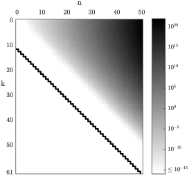
Fig. 1: Error growth when recursing using (18c). The entries of $R$ below the dark line are exactly zero.

The calculation of $R$ could have been as easy as suggested by Theorem 5: calculate the zeroth column of $R$ following (17) and recurse using (18a), (18b), and (18c). Unfortunately, (18c) is not numerically stable even in absolute sense.

Example 1: To see the instability, we take a randomly generated Chebyshev series of degree $10$, i.e. $f_{M}=\sum_{m=0}^{10}a_{m}T_{m}(x)$, with $|a_{m}|\leqslant 1$ and compare the entries in columns $1$ to $50$ calculated recursively using Theorem 5 with the exact values computed symbolically using Mathematica. Figure 1 shows the entrywise absolute error. The error in the entries above the main diagonal grows very rapidly, which is similar to what is observed in [13] for the Legendre case. In fact, the rounding errors in $R_{k-1,n}$ and $R_{k+1,n}$ in (18c) are subject to an amplification by the factor $(n+1)/k$, which is larger than $1$ above the main diagonal. The recursion snowballs the errors introduced in each use of (18c) very quickly, resulting in the computed values soon to become totally garbage. In the worst scenario, an error could be magnified $n$ folds in the $n$-th recursion and blows up at a rate of factorial. For instance, the absolute error in the entry at the top right corner of $R$ in Figure 1, i.e. $R_{0,50}$, is $\mathcal{O}(10^{20})$, while the true value is about $10^{-3}$ in this example.

Indeed, (18c) is only useful for calculating the entries on and below the main diagonal, that is, the entries in the region labeled by $A$ in Figure 2. To circumvent the instability, we make the following critical observation which is similar to the one made in [13] for the Legendre-based convolution matrices (see Section 4.1.1).

Theorem 6 (Symmetry of $R$).

For $M+1\leqslant k,n\leqslant N$,

(20) $$R_{n,k}=\frac{(-1)^{n+k}k}{n}R_{k,n}.$$

We find it easy to prove Theorem 6 by deducing it from the analogous result of the Jacobi-based convolution matrices and, therefore, defer the proof to Section 4.2.

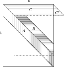
Fig. 2: The convolution matrix $R$ defined by an $M$-Chebyshev series is an almost-banded matrix with bandwidth $M+1$ plus $M+1$ rows at the top. The construction of $R$ starts in region $A$ (the main diagonal and the first $M+1$ subdiagonals) by recursion from the left to the right using (18a), (18b), and (18c). The entries in region $B$ (the first $M+1$ superdiagonals), are obtained by symmetry (20). With the padding region $C^{p}$, the recast recurrence relation (21) allows a stable recursion for entries in region $C$ (the top $M+1$ rows). All remaining entries are exact zeros.

Theorem 6 shows the symmetry of $R$ up to a scaling factor, apart from the top and the bottom $M+1$ rows and the first $M+1$ columns. In Figure 2, the symmetric part of $R$ is marked by the dashed lines. The important implications of this symmetry are (1) this $(N-M)\times(N-M)$ symmetric submatrix of $R$ is banded with bandwidth $M+1$; (2) the entries in region $B$ can be obtained stably and cheaply by rescaling their mirror images about the main diagonal; (3) the entries of the top $M+1$ rows of $R$, i.e. region $C$, can then be calculated by the same recurrence relation given by (18c).

When (18c) is used to calculate the entries in the top $M+1$ rows, we rewrite it so that calculation is done by rows, going upward from the bottom of region $C$ to the top:

(21) $$R^{\prime\prime}_{k-1,n}=-\frac{2k(-1)^{n}}{n^{2}-1}R_{k,0}-\frac{k}{n-1}R_{k,n-1}+\frac{k}{n+1}R_{k,n+1}+R_{k+1,n},$$

where the double prime indicates that the term is halved when $k=1$. This new recurrence relation is numerically stable in region $C$. In contrast to (18c), the rounding errors are now premultiplied by $k/(n-1)$ or $k/(n+1)$, which are less than or, at most, equal to $1$ above the main diagonal. Therefore, the rounding errors are diminished in the course of recursion, rather than amplified.

It is worth noting that when recursing for the top $M+1$ rows using (21), we have to start with entries beyond the first $N+1$ columns of $R$, so that all entries in the “domain of dependence” of the zeroth row are counted on. This suggests a triangle-shaped padding region, labeled by $C^{p}$ in Figure 2.

We summarize the stable algorithm described above as follows:

Algorithm 1 Construction of the convolution matrix $R$

1:  Construct the non-zero entries in the zeroth column $R_{:,0}$ using (17).

2:  Calculate the non-zero entries on and below the main diagonal (Region A) using (18a), (18b), and (18c).

3:  Calculate the non-zero entries above the main diagonal (Region B) in rows $M+1$ to $N$ using (20).

4:  Recurse for the entries above the main diagonal in the top $M+1$ rows (Region C) using (21).

Example 2: Now we re-compute the same $R$ in Example 1 using Algorithm 1 and plot the entrywise absolute error in Figure 3(a). With the stabilized algorithm, the maximum error across all the entries is now $2.12\times 10^{-16}$ in this example.

Example 3: In Figure 3(b), we show a similar example with $M=1000$ and $N=5000$. Again, $\underline{a}$ is generated randomly with $|a_{m}|\leqslant 1$. The largest entrywise error across all the entries of $R$ is $1.28\times 10^{-15}$.

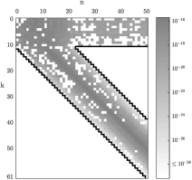
(a) $M=10$ , $N=50$.

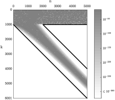
(b) $M=1000$, $N=5000$.

Fig. 3: Entrywise error of the nonzero entries of $R$ obtained using Algorithm 1. The dark lines circumscribe the region outside which entries are exact zeros.

A curious observation we made in the last two examples and other experiments that we carried out is that the magnitudes of the entries in a convolution matrix have an enormous range of orders. In Example 2, even though the entries of $\underline{a}$ are all $\mathcal{O}(10^{-1})$, the exact values obtained symbolically using Mathematica show that some entries of $R$ can be as small as $\mathcal{O}(10^{-14})$. Therefore, it makes little sense to talk about the relative error of the computed entries, since we cannot expect to be able to compute $\mathcal{O}(10^{-14})$ values accurately in a relative sense by using $\mathcal{O}(10^{-1})$ data in floating point arithmetic.

In Example 3, the magnitudes of the entries vary from $\mathcal{O}(10^{-1})$ to $\mathcal{O}(10^{p})$ with $p<-324$. The most minuscule entries are not even representable by the IEEE floating point arithmetic [16]. This also suggests that we should confine our discussion to absolute accuracy only.

Although the gargantuan discrepancy in the magnitudes of the entries denies any attempt to compute them accurately in a relative sense, the convolution matrices constructed using our stable algorithm give accurate approximations to the convolution operators in the absolute sense and work perfectly fine when used for calculating $h_{M+N+1}(x)$ or solving convolution integral equations, since it is also only sensible to discuss absolute accuracy in these cases.

We close this section with a classic example from the renewal theory [4, Example 1.4.3], [10].

Example 4: It can be shown that the Volterra convolution integral equation

(22) $$u(x)=f(x)+\int_{0}^{x}f(x-t)u(t)\>dt,\qquad x\in[0,2],$$

where the convolution kernel

(23) $$f(x)=\frac{1}{2}x^{2}e^{-x},$$

has a unique solution

(24) $$u(x)=\frac{1}{3}-\frac{1}{3}\left(\cos\frac{\sqrt{3}}{2}x+\sqrt{3}\sin\frac{\sqrt{3}}{2}x\right)e^{-3x/2}.$$

We first test the use of convolution matrices as a means of approximating the convolution function $h(x)$. To do so, we approximate $f(x)$ and $u(x)$ by Chebyshev series $f_{M}(x)$ and $u_{N}(x)$ of degrees $16$ and $17$, respectively, to machine precision uniformly on $[0,2]$and then form the convolution matrix $R$ using the Chebyshev coefficients $\underline{c}^{f}$ of $f_{M}(x)$. The product of $R$ and $u_{N}(x)$’s Chebyshev coefficients $\underline{c}^{u}$ returns us the Chebyshev coefficients of $h_{M+N+1}(x)=(f*u)(x)$, which should be a good approximation of $u(x)-f(x)$. Indeed, the pointwise absolute error in $h_{M+N+1}(x)$ is displayed in Figure 4(a), where the largest error is approximately $1.10\times 10^{-16}$.

Next, we take $u(x)$ as unknown and solve for $\underline{c}^{u}$ with the knowledge of $f_{M}(x)$. This examines the use of convolution matrices in solving convolution integral equations. We construct the $(N+18)\times(N+1)$ convolution matrix for $N=1,3,5,\ldots,25$ and denote by $R^{N}$ the square matrix formed by the first $N+1$ rows. Solving

$$(I-R^{N})\underline{c}^{u}=\underline{c}^{fN}$$

gives us $\underline{c}^{u}$, where $\underline{c}^{fN}$ is a tailored version of $\underline{c}^{f}$, either by truncation or zero-padding so that it is of length $N+1$. Figure 4(b) shows the maximum pointwise error of $u_{N}(x)=\sum_{n=0}^{N}c^{u}_{n}T_{n}(x)$ for increasing $N$. What we see is a spectral convergence as the size of discretization increases. When $N=17$, the largest pointwise error in $[0,2]$ decays to $1.39\times 10^{-16}$, effectively of machine precision.

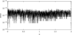
(a)

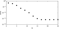
(b)

Fig. 4: An example from renewal theory: (a) The pointwise error of the computed Chebyshev approximant to the convolution integral on the right-hand side of (22). (b) Spectral convergence of the computed approximant to $u(x)$ in (22) using convolution matrices of increasing sizes.

4 Other classical orthogonal polynomials

To derive the recurrence relations in Sections 2 and 3, we have only used the properties of Chebyshev polynomials that are also shared by other classical orthogonal polynomials. It is, therefore, natural to see how the results in the last two sections extend to Gegenbauer and Jacobi spaces. For convergence theory of Gegenbauer and Jacobi approximants, see, for example, [28, 29, 31].

4.1 Convolution matrices in Gegenbauer space

Gegenbauer polynomials $C_{n}^{(\lambda)}(x)$, also known as ultraspherical polynomials, can be defined using the three-term recurrence relation [25, §4.7]

(25) $$2(n+\lambda)xC_{n}^{(\lambda)}(x)=(n+1)C_{n+1}^{(\lambda)}(x)+(n+2\lambda-1)C_{n-1}^{(\lambda)}(x)$$

with $C_{-1}^{(\lambda)}(x)=0$ and $C_{0}^{(\lambda)}(x)=1$, under the constraints $\lambda>-1/2$ and $\lambda\neq 0$. The following lemma, parallel to Lemma 1, can be derived using (25).

Lemma 7.

For any integer $n$, Gegenbauer polynomials satisfy the following recurrence relation that can be written in derivative or integral forms:

(26) $$\begin{array}[]{l}\begin{aligned} 2(n+\lambda)C_{n}^{(\lambda)}(x)=\frac{\mathrm{d}}{\mathrm{d}x}\left(C_{n+1}^{(\lambda)}(x)-C_{n-1}^{(\lambda)}(x)\right),\\ \int C_{n}^{(\lambda)}(t)\mathrm{d}t=\frac{1}{2(n+\lambda)}\left(C_{n+1}^{(\lambda)}(x)-C_{n-1}^{(\lambda)}(x)\right),\end{aligned}\end{array}$$

where $C^{\lambda}_{n}(x)=0$ for $n<0$.

Proof.

See [25, §4.7]. ∎

We omit the proofs for the next two theorems as they are analogous to those of Theorems 2, 4, and 5.

Theorem 8 (Recurrence of convolutions of Gegenbauer polynomials).

For Gegenbauer series $f_{M}(x)=\sum_{m=0}^{M}a_{m}C^{(\lambda)}_{m}(x)$,

(27) $$\int_{-1}^{y}f_{M}(x-t)C_{0}^{(\lambda)}(t)\mathrm{d}t=\int_{-1}^{y}f_{M}(t)\mathrm{d}t$$

and the convolutions of $f_{M}(x)$ and $C^{(\lambda)}_{n}(x)$ recurse:

(28) $$\begin{multlined}\int_{-1}^{y}f_{M}(x-t)C_{n+1}^{(\lambda)}(t)\mathrm{d}t=2(n+\lambda)\int_{-1}^{y}\int_{-1}^{x+1}f_{M}(x-t)C_{n}^{(\lambda)}(t)\mathrm{d}t\,\mathrm{d}(x+1)\\ +\int_{-1}^{y}f_{M}(x-t)C_{n-1}^{(\lambda)}(t)\mathrm{d}t+S^{(\lambda)}_{n}\int_{-1}^{y}f_{M}(t)\mathrm{d}t,\end{multlined}\int_{-1}^{y}f_{M}(x-t)C_{n+1}^{(\lambda)}(t)\mathrm{d}t=2(n+\lambda)\int_{-1}^{y}\int_{-1}^{x+1}f_{M}(x-t)C_{n}^{(\lambda)}(t)\mathrm{d}t\,\mathrm{d}(x+1)\\ +\int_{-1}^{y}f_{M}(x-t)C_{n-1}^{(\lambda)}(t)\mathrm{d}t+S^{(\lambda)}_{n}\int_{-1}^{y}f_{M}(t)\mathrm{d}t,$$

where $x\in[-2,0]$, $y=x+1\in[-1,1]$ and

(29) $$S^{(\lambda)}_{n}=\frac{2(-1)^{n+1}(\lambda+n)(2\lambda-1)_{n}}{(n+1)!},$$

where $(\cdot)_{n}$ is the Pochhammer symbol for ascending factorial with $(a)_{n}\coloneqq a(a+1)(a+2)\cdots(a+n-1)$ and $(a)_{0}\coloneqq 1$.

Theorem 9 (Construction of $R^{(\lambda)}$).

The entries of the zeroth column of $R^{(\lambda)}$ are

(30a) $$R^{(\lambda)}_{k,0}=\begin{cases}0&\quad k>M+1,\\[5.69054pt] \displaystyle\frac{a_{k-1}}{2(k+\lambda-1)}-\frac{a_{k+1}}{2(k+\lambda+1)}&\quad 1\leqslant k\leqslant M+1,\\[11.38109pt] \displaystyle\sum_{j=1}^{M+1}(-1)^{j+1}\frac{(2\lambda)_{j}}{j!}R^{(\lambda)}_{j,0}&\quad k=0,\end{cases}$$

with $$a_{M+1}=a_{M+2}=0 n\geqslant 0$$. For ,

(30b) $$R^{(\lambda)}_{k,n+1}=S^{(\lambda)}_{n}R^{(\lambda)}_{k,0}+R^{(\lambda)}_{k,n-1}+\frac{n+\lambda}{k+\lambda-1}R^{(\lambda)}_{k-1,n}-\frac{n+\lambda}{k+\lambda+1}R^{(\lambda)}_{k+1,n},$$

where $R^{(\lambda)}_{:,-1}$ are understood to be zeros.

Similar to the Chebyshev case, the Gegenbauer-based convolution matrices are also almost-banded with a symmetric submatrix.

Theorem 10 (Symmetry of $R^{(\lambda)}$).

For $M+1\leqslant k,n\leqslant N$,

(31) $$R^{(\lambda)}_{k,n}=(-1)^{k+n}\frac{k+\lambda}{n+\lambda}R^{(\lambda)}_{n,k}.$$

Again, we defer the proof to Section 4.2.

Same stability issue occurs if Gegenbauer-based convolution matrices are constructed naively using (30b). The stable algorithm is given in Algorithm 2. Analogously, we need to recast (30b) before it can be used for calculating the entries above the main diagonal:

(32) $$R^{(\lambda)}_{k-1,n}=\frac{k+\lambda-1}{n+\lambda}\left(-S^{(\lambda)}_{n}R^{(\lambda)}_{k,0}+R^{(\lambda)}_{k,n+1}-R^{(\lambda)}_{k,n-1}\right)+\frac{k+\lambda-1}{k+\lambda+1}R^{(\lambda)}_{k+1,n}.$$

4.1.1 Convolution matrices in Legendre space

Gegenbauer polynomials reduce to Legendre polynomials $P_{n}(x)$ when $\lambda=1/2$, i.e. $P_{n}(x)=C_{n}^{(1/2)}(x)$. In this case, $S^{(1/2)}_{n}=0$ , annihilating the last term in (28) and the first term on the right-hand side of (30b). Now (30b) reduces to a four-term recurrence relation

(33) $$R^{(1/2)}_{k,n+1}=R^{(1/2)}_{k,n-1}+\frac{2n+1}{2k-1}R^{(1/2)}_{k-1,n}-\frac{2n+1}{2k+3}R^{(1/2)}_{k+1,n},$$

which is exactly the one found in [13] via spherical Bessel functions.

In the absence of the $R^{(\lambda)}_{k,0}$ term, symmetry (31) extends beyond the submatrix $R^{(\lambda)}_{M+1:N,M+1:N}$ as the entire matrix is symmetric up to a scaling factor. Hence, Legendre-based convolution matrices are exactly banded with bandwidth $M+1$ and this is the only case where polynomial-based convolution matrices are exactly banded.

4.2 Convolution matrices in Jacobi space

For Jacobi polynomials, we adopt the most commonly-used normalization, which can be found, for example, in [25, §4.2.1]. In terms of hypergeometric function, they are

(34) $$P_{n}^{(\alpha,\beta)}(x)=\frac{(\alpha+1)_{n}}{n!}{}_{2}F_{1}\left(\begin{array}[]{c}-n,n+\alpha+\beta+1\\ \alpha+1\end{array};\frac{1-x}{2}\right),~{}~{}~{}n\geqslant 0,$$

for $\alpha,\beta>-1$.

We first introduce a similar recurrence for the derivatives and the integrals of Jacobi polynomials, analogous to (7b) for Chebyshev polynomials and (26) for Gegenbauer polynomials, but with one extra term.

Lemma 11.

For any integer $n$, Jacobi polynomials $P^{(\alpha,\beta)}_{n}(x)$ satisfy the following recurrence relation which can be written in derivative or integral forms:

(35a) $$~{}~{}~{}~{}~{}~{}P_{n}^{(\alpha,\beta)}(x)=A^{(\alpha,\beta)}_{n+1}\frac{\mathrm{d}}{\mathrm{d}x}P_{n+1}^{(\alpha,\beta)}(x)+B^{(\alpha,\beta)}_{n}\frac{\mathrm{d}}{\mathrm{d}x}P_{n}^{(\alpha,\beta)}(x)+C^{(\alpha,\beta)}_{n-1}\frac{\mathrm{d}}{\mathrm{d}x}P_{n-1}^{(\alpha,\beta)}(x),$$

(35b) $$\int P_{n}^{(\alpha,\beta)}(x)\mathrm{d}x=A^{(\alpha,\beta)}_{n+1}P_{n+1}^{(\alpha,\beta)}(x)+B^{(\alpha,\beta)}_{n}P_{n}^{(\alpha,\beta)}(x)+C^{(\alpha,\beta)}_{n-1}P_{n-1}^{(\alpha,\beta)}(x),$$

where

(35c) $$A^{(\alpha,\beta)}_{n+1} =\frac{2(\alpha+\beta+n+1)}{(\alpha+\beta+2n+1)(\alpha+\beta+2n+2)},$$

(35d) $$B^{(\alpha,\beta)}_{n} =\frac{2(\alpha-\beta)}{(\alpha+\beta+2n)(\alpha+\beta+2n+2)},$$

(35e) $$C^{(\alpha,\beta)}_{n-1} =-\frac{2(\alpha+n)(\beta+n)}{(\alpha+\beta+n)(\alpha+\beta+2n)(\alpha+\beta+2n+1)}.$$

Here, we assume $P_{n}^{(\alpha,\beta)}(x)=0$ for $n<0$.

Proof.

See, for example, [21, Theorem 3.23]. ∎

Different from (7b) or (26), (35a) and (35b) both have a middle term on the right-hand side, indexed with $n$. In the symmetric case when $\alpha=\beta$, $B_{n}^{(\alpha,\beta)}$ becomes zero and this middle term vanishes.

Analogous to Theorem 2 and Theorem 8, a recurrence relation for the convolutions of a Jacobi series with Jacobi polynomials can be derived using (35a).

Theorem 12 (Recurrence of convolutions of Jacobi polynomials).

For Jacobi series $f_{M}(x)=\sum_{m=0}^{M}a_{m}P^{(\alpha,\beta)}_{m}(x)$,

(36) $$\begin{multlined}\int_{-1}^{y}f_{M}(x-t)P^{(\alpha,\beta)}_{n+1}(t)\mathrm{d}t=-\frac{1}{A^{(\alpha,\beta)}_{n+1}}\int_{-1}^{y}\int_{-1}^{x+1}f_{M}(x-t)P^{(\alpha,\beta)}_{n}(t)\mathrm{d}t\,\mathrm{d}(x+1)\\ -\frac{B^{(\alpha,\beta)}_{n}}{A^{(\alpha,\beta)}_{n+1}}\int_{-1}^{y}f_{M}(x-t)P^{(\alpha,\beta)}_{n}(t)\mathrm{d}t-\frac{C^{(\alpha,\beta)}_{n-1}}{A^{(\alpha,\beta)}_{n+1}}\int_{-1}^{y}f_{M}(x-t)P^{(\alpha,\beta)}_{n-1}(t)\mathrm{d}t\\ +\frac{S^{(\alpha,\beta)}_{n}}{A^{(\alpha,\beta)}_{n+1}}\int_{-1}^{y}f_{M}(t)\mathrm{d}t,\end{multlined}\int_{-1}^{y}f_{M}(x-t)P^{(\alpha,\beta)}_{n+1}(t)\mathrm{d}t=-\frac{1}{A^{(\alpha,\beta)}_{n+1}}\int_{-1}^{y}\int_{-1}^{x+1}f_{M}(x-t)P^{(\alpha,\beta)}_{n}(t)\mathrm{d}t\,\mathrm{d}(x+1)\\ -\frac{B^{(\alpha,\beta)}_{n}}{A^{(\alpha,\beta)}_{n+1}}\int_{-1}^{y}f_{M}(x-t)P^{(\alpha,\beta)}_{n}(t)\mathrm{d}t-\frac{C^{(\alpha,\beta)}_{n-1}}{A^{(\alpha,\beta)}_{n+1}}\int_{-1}^{y}f_{M}(x-t)P^{(\alpha,\beta)}_{n-1}(t)\mathrm{d}t\\ +\frac{S^{(\alpha,\beta)}_{n}}{A^{(\alpha,\beta)}_{n+1}}\int_{-1}^{y}f_{M}(t)\mathrm{d}t,$$

where $x\in[-2,0]$, $y=x+1\in[-1,1]$, and

(37) $$S^{(\alpha,\beta)}_{n}=\frac{2(-1)^{n+1}(\beta)_{n+1}}{(\alpha+\beta+n)(n+1)!}.$$

Note that the second term on the right-hand side accounts for the middle term in (35a). Recognizing the convolutions in (36) as Jacobi series and then applying (35b) to the first term on the right-hand side, we obtain the recurrence relation for the entries of a Jacobi convolution matrix $R^{(\alpha,\beta)}$.

Theorem 13 (Construction of $R^{(\alpha,\beta)}$).

The entries of the zeroth column of $R^{(\alpha,\beta)}$ are

(38a) $$R^{(\alpha,\beta)}_{k,0}=\begin{cases}0&\quad k>M+1,\\[5.69054pt] \displaystyle A^{(\alpha,\beta)}_{k}a_{k-1}+B^{(\alpha,\beta)}_{k}a_{k}+C^{(\alpha,\beta)}_{k}a_{k+1}&\quad 1\leqslant k\leqslant M+1,\\[5.69054pt] \displaystyle\sum_{j=1}^{M+1}(-1)^{j+1}\frac{(\beta+1)_{j}}{j!}R^{(\alpha,\beta)}_{j,0}&\quad k=0,\end{cases}$$

with $$a_{M+1}=a_{M+2}=0 n\geqslant 0$$. For ,

(38b) $$\begin{multlined}R^{(\alpha,\beta)}_{k,n+1}=\frac{B^{(\alpha,\beta)}_{k}-B^{(\alpha,\beta)}_{n}}{A^{(\alpha,\beta)}_{n+1}}R^{(\alpha,\beta)}_{k,n}-\frac{C^{(\alpha,\beta)}_{n-1}}{A^{(\alpha,\beta)}_{n+1}}R^{(\alpha,\beta)}_{k,n-1}+\frac{A^{(\alpha,\beta)}_{k}}{A^{(\alpha,\beta)}_{n+1}}R^{(\alpha,\beta)}_{k-1,n}\\ +\frac{C^{(\alpha,\beta)}_{k}}{A^{(\alpha,\beta)}_{n+1}}R^{(\alpha,\beta)}_{k+1,n}+\frac{S^{(\alpha,\beta)}_{n}}{A^{(\alpha,\beta)}_{n+1}}R^{(\alpha,\beta)}_{k,0},\end{multlined}R^{(\alpha,\beta)}_{k,n+1}=\frac{B^{(\alpha,\beta)}_{k}-B^{(\alpha,\beta)}_{n}}{A^{(\alpha,\beta)}_{n+1}}R^{(\alpha,\beta)}_{k,n}-\frac{C^{(\alpha,\beta)}_{n-1}}{A^{(\alpha,\beta)}_{n+1}}R^{(\alpha,\beta)}_{k,n-1}+\frac{A^{(\alpha,\beta)}_{k}}{A^{(\alpha,\beta)}_{n+1}}R^{(\alpha,\beta)}_{k-1,n}\\ +\frac{C^{(\alpha,\beta)}_{k}}{A^{(\alpha,\beta)}_{n+1}}R^{(\alpha,\beta)}_{k+1,n}+\frac{S^{(\alpha,\beta)}_{n}}{A^{(\alpha,\beta)}_{n+1}}R^{(\alpha,\beta)}_{k,0},$$

where $R^{(\alpha,\beta)}_{:,-1}$ are understood to be zeros.

Again, the same stability issue holds us from constructing the Jacobi-based convolution matrices by using (38b) directly. Fortunately, the symmetry persists though the recurrence relation (38b) is augmented by the extra $R^{(\alpha,\beta)}_{k,n}$ term. Thus, the Jacobi-based convolution matrices are almost-banded too. Now, we are in a position to show the symmetry of the Jacobi-based convolution matrices, from which the symmetric properties of the Chebyshev- and Gegenbauer-based convolution matrices can be easily deduced.

Theorem 14 (Symmetry of $R^{(\alpha,\beta)}$).

For $M+1\leqslant k,n\leqslant N$,

(39) $$R_{n,k}^{(\alpha,\beta)}=(-1)^{k+n}\frac{(\alpha+\beta+2n+1)(\alpha+1)_{k}(\beta+1)_{k}\Big{(}(\alpha+\beta+1)_{n}\Big{)}^{2}}{(\alpha+\beta+2k+1)(\alpha+1)_{n}(\beta+1)_{n}\Big{(}(\alpha+\beta+1)_{k}\Big{)}^{2}}R_{k,n}^{(\alpha,\beta)}.$$

Proof.

For $k\geqslant M+2$, (38b) reduces to

(40) $$\begin{multlined}\frac{A^{(\alpha,\beta)}_{n+1}}{B^{(\alpha,\beta)}_{k}-B^{(\alpha,\beta)}_{n}}R^{(\alpha,\beta)}_{k,n+1}+\frac{C^{(\alpha,\beta)}_{n-1}}{B^{(\alpha,\beta)}_{k}-B^{(\alpha,\beta)}_{n}}R^{(\alpha,\beta)}_{k,n-1}-R^{(\alpha,\beta)}_{k,n}\\ -\frac{A^{(\alpha,\beta)}_{k}}{B^{(\alpha,\beta)}_{k}-B^{(\alpha,\beta)}_{n}}R^{(\alpha,\beta)}_{k-1,n}-\frac{C^{(\alpha,\beta)}_{k}}{B^{(\alpha,\beta)}_{k}-B^{(\alpha,\beta)}_{n}}R^{(\alpha,\beta)}_{k+1,n}=0,\end{multlined}\frac{A^{(\alpha,\beta)}_{n+1}}{B^{(\alpha,\beta)}_{k}-B^{(\alpha,\beta)}_{n}}R^{(\alpha,\beta)}_{k,n+1}+\frac{C^{(\alpha,\beta)}_{n-1}}{B^{(\alpha,\beta)}_{k}-B^{(\alpha,\beta)}_{n}}R^{(\alpha,\beta)}_{k,n-1}-R^{(\alpha,\beta)}_{k,n}\\ -\frac{A^{(\alpha,\beta)}_{k}}{B^{(\alpha,\beta)}_{k}-B^{(\alpha,\beta)}_{n}}R^{(\alpha,\beta)}_{k-1,n}-\frac{C^{(\alpha,\beta)}_{k}}{B^{(\alpha,\beta)}_{k}-B^{(\alpha,\beta)}_{n}}R^{(\alpha,\beta)}_{k+1,n}=0,$$

since $R^{(\alpha,\beta)}_{k,0}=0$ when $k\geqslant M+2$.

Noting that $R^{(\alpha,\beta)}_{k,n}$ is a rational function of $n$, $k$, and $\underline{a}$, we denote the ratio of $R^{(\alpha,\beta)}_{k,n}$ and $R^{(\alpha,\beta)}_{n,k}$ by $r(n,k,\underline{a})$, that is,

(41) $$R^{(\alpha,\beta)}_{k,n}=r(n,k,\underline{a})R^{(\alpha,\beta)}_{n,k},$$

with $r(n,n,\underline{a})=1$.

Substituting (41) into (40) and dividing all terms by $r(n,k,\underline{a})$, we have

$$\begin{multlined}\frac{A^{(\alpha,\beta)}_{n+1}}{B^{(\alpha,\beta)}_{k}-B^{(\alpha,\beta)}_{n}}\frac{r(n+1,k,\underline{a})}{r(n,k,\underline{a})}R^{(\alpha,\beta)}_{n+1,k}+\frac{C^{(\alpha,\beta)}_{n-1}}{B^{(\alpha,\beta)}_{k}-B^{(\alpha,\beta)}_{n}}\frac{r(n-1,k,\underline{a})}{r(n,k,\underline{a})}R^{(\alpha,\beta)}_{n-1,k}-R^{(\alpha,\beta)}_{n,k}\\ -\frac{A^{(\alpha,\beta)}_{k}}{B^{(\alpha,\beta)}_{k}-B^{(\alpha,\beta)}_{n}}\frac{r(n,k-1,\underline{a})}{r(n,k,\underline{a})}R^{(\alpha,\beta)}_{n,k-1}-\frac{C^{(\alpha,\beta)}_{k}}{B^{(\alpha,\beta)}_{k}-B^{(\alpha,\beta)}_{n}}\frac{r(n,k+1,\underline{a})}{r(n,k,\underline{a})}R^{(\alpha,\beta)}_{n,k+1}=0.\end{multlined}\frac{A^{(\alpha,\beta)}_{n+1}}{B^{(\alpha,\beta)}_{k}-B^{(\alpha,\beta)}_{n}}\frac{r(n+1,k,\underline{a})}{r(n,k,\underline{a})}R^{(\alpha,\beta)}_{n+1,k}+\frac{C^{(\alpha,\beta)}_{n-1}}{B^{(\alpha,\beta)}_{k}-B^{(\alpha,\beta)}_{n}}\frac{r(n-1,k,\underline{a})}{r(n,k,\underline{a})}R^{(\alpha,\beta)}_{n-1,k}-R^{(\alpha,\beta)}_{n,k}\\ -\frac{A^{(\alpha,\beta)}_{k}}{B^{(\alpha,\beta)}_{k}-B^{(\alpha,\beta)}_{n}}\frac{r(n,k-1,\underline{a})}{r(n,k,\underline{a})}R^{(\alpha,\beta)}_{n,k-1}-\frac{C^{(\alpha,\beta)}_{k}}{B^{(\alpha,\beta)}_{k}-B^{(\alpha,\beta)}_{n}}\frac{r(n,k+1,\underline{a})}{r(n,k,\underline{a})}R^{(\alpha,\beta)}_{n,k+1}=0.$$

Now, swapping $k$ and $n$ in (40) gives

$$\begin{multlined}\frac{A^{(\alpha,\beta)}_{k+1}}{B^{(\alpha,\beta)}_{n}-B^{(\alpha,\beta)}_{k}}R^{(\alpha,\beta)}_{n,k+1}+\frac{C^{(\alpha,\beta)}_{k-1}}{B^{(\alpha,\beta)}_{n}-B^{(\alpha,\beta)}_{k}}R^{(\alpha,\beta)}_{n,k-1}-R^{(\alpha,\beta)}_{n,k}\\ -\frac{A^{(\alpha,\beta)}_{n}}{B^{(\alpha,\beta)}_{n}-B^{(\alpha,\beta)}_{k}}R^{(\alpha,\beta)}_{n-1,k}-\frac{C^{(\alpha,\beta)}_{n}}{B^{(\alpha,\beta)}_{n}-B^{(\alpha,\beta)}_{k}}R^{(\alpha,\beta)}_{n+1,k}=0.\end{multlined}\frac{A^{(\alpha,\beta)}_{k+1}}{B^{(\alpha,\beta)}_{n}-B^{(\alpha,\beta)}_{k}}R^{(\alpha,\beta)}_{n,k+1}+\frac{C^{(\alpha,\beta)}_{k-1}}{B^{(\alpha,\beta)}_{n}-B^{(\alpha,\beta)}_{k}}R^{(\alpha,\beta)}_{n,k-1}-R^{(\alpha,\beta)}_{n,k}\\ -\frac{A^{(\alpha,\beta)}_{n}}{B^{(\alpha,\beta)}_{n}-B^{(\alpha,\beta)}_{k}}R^{(\alpha,\beta)}_{n-1,k}-\frac{C^{(\alpha,\beta)}_{n}}{B^{(\alpha,\beta)}_{n}-B^{(\alpha,\beta)}_{k}}R^{(\alpha,\beta)}_{n+1,k}=0.$$

Matching the terms in the last two equations, we obtain two recurrence relations for $r(n,k,\underline{a})$

$$\frac{r(n,k+1,\underline{a})}{r(n,k,\underline{a})}=\frac{A^{(\alpha,\beta)}_{k+1}}{C^{(\alpha,\beta)}_{k}}\quad\mbox{and}\quad\frac{r(n+1,k,\underline{a})}{r(n,k,\underline{a})}=\frac{C^{(\alpha,\beta)}_{n}}{A^{(\alpha,\beta)}_{n+1}}$$

for any $n,k\geqslant M+1$. Therefore,

$$r(n,k,\underline{a})=r(n,M+1,\underline{a})\prod_{j=M+1}^{k-1}\frac{A^{(\alpha,\beta)}_{j+1}}{C^{(\alpha,\beta)}_{j}}$$

and $$r(n,M+1,\underline{a})=r(M+1,M+1,\underline{a})\prod_{j=M+1}^{n-1}\frac{C^{(\alpha,\beta)}_{j}}{A^{(\alpha,\beta)}_{j+1}},$$

which, combined, give

(42) $$r(n,k,\underline{a})=\left(\prod_{j=0}^{n-1}\frac{C^{(\alpha,\beta)}_{j}}{A^{(\alpha,\beta)}_{j+1}}\right)\left(\prod_{j=0}^{k-1}\frac{A^{(\alpha,\beta)}_{j+1}}{C^{(\alpha,\beta)}_{j}}\right),$$

where $r(M+1,M+1,\underline{a})=1$ is used. Substituting (35d) in gives (39). ∎

Now we are ready to show Theorems 6 and 10.

Proof of Theorem 6.

Taking the limit of (39) as $\alpha,\beta\to-1/2$, we have

(43) $$R_{n,k}^{(-\frac{1}{2},-\frac{1}{2})}=(-1)^{n+k}\frac{k}{n}\displaystyle\frac{\left(\left(\frac{1}{2}\right)_{k}\right)^{2}\left(n!\right)^{2}}{\left(\left(\frac{1}{2}\right)_{n}\right)^{2}\left(k!\right)^{2}}\ R_{k,n}^{(-\frac{1}{2},-\frac{1}{2})}.$$

Relating Chebyshev polynomial $T_{n}(x)$ to Jacobi polynomial $P^{(-1/2,-1/2)}_{n}(x)$ by

(44) $$P_{n}^{(-\frac{1}{2},-\frac{1}{2})}(x)=\frac{\left(\frac{1}{2}\right)_{n}}{n!}T_{n}(x),$$

we obtain

(45) $$R_{k,n}^{(-\frac{1}{2},-\frac{1}{2})}=\frac{\left(\frac{1}{2}\right)_{n}k!}{\left(\frac{1}{2}\right)_{k}n!}R_{k,n}$$

for any $k,n\geqslant 0$. Finally, substituting (45) into (43) gives (20). ∎

Proof of Theorem 10.

The limit of (39) as $\alpha,\beta\to\lambda-1/2$ is

(46) $$R_{n,k}^{(\lambda-\frac{1}{2},\lambda-\frac{1}{2})}=(-1)^{k+n}\frac{\lambda+n}{\lambda+k}\frac{\left((2\lambda)_{n}\right)^{2}\left(\left(\lambda+\frac{1}{2}\right)_{k}\right)^{2}}{\left((2\lambda)_{k}\right)^{2}\left(\left(\lambda+\frac{1}{2}\right)_{n}\right)^{2}}R_{k,n}^{(\lambda-\frac{1}{2},\lambda-\frac{1}{2})}$$

With the scaling between $C_{n}^{(\lambda)}$ and $P_{n}^{(\lambda-1/2,\lambda-1/2)}$

$$P_{n}^{(\lambda-\frac{1}{2},\lambda-\frac{1}{2})}=\frac{\left(\lambda+\frac{1}{2}\right)_{n}}{\left(2\lambda\right)_{n}}C_{n}^{(\lambda)}(x),$$

we have

(47) $$R_{k,n}^{(\lambda-\frac{1}{2},\lambda-\frac{1}{2})}=\frac{\left(\lambda+\frac{1}{2}\right)_{k}(2\lambda)_{n}}{(2\lambda)_{k}\left(\lambda+\frac{1}{2}\right)_{n}}R_{k,n}^{(\lambda)}$$

for all $k,n\geqslant 0$. Combining (47) and (46) yields (31). ∎

The symmetric relation (39) cannot be used directly due to the arithmetic overflow for large $k$ and $n$. Instead, we cancel the common factors in the numerator and the denominator and match up the factors of similar magnitude to obtain an equivalent, but numerically more manageable formula by noting that (39) is only needed for $k>n$:

(48) $$R_{n,k}^{(\alpha,\beta)}=(-1)^{k+n}\frac{\alpha+\beta+2n+1}{\alpha+\beta+2k+1}\prod_{j=n}^{k-1}\frac{j+\alpha+1}{j+\alpha+\beta+1}\prod_{j=n}^{k-1}\frac{j+\beta+1}{j+\alpha+\beta+1}R_{k,n}^{(\alpha,\beta)}.$$

When we recurse for the top rows, we need to rewrite (38b) as we do for the Chebyshev and Gegenbauer cases:

(49) $$\begin{multlined}R^{(\alpha,\beta)}_{k-1,n}=\frac{B^{(\alpha,\beta)}_{n}-B^{(\alpha,\beta)}_{k}}{A^{(\alpha,\beta)}_{k}}R^{(\alpha,\beta)}_{k,n}+\frac{C^{(\alpha,\beta)}_{n-1}}{A^{(\alpha,\beta)}_{k}}R^{(\alpha,\beta)}_{k,n-1}+\frac{A^{(\alpha,\beta)}_{n+1}}{A^{(\alpha,\beta)}_{k}}R^{(\alpha,\beta)}_{k,n+1}\\ -\frac{C^{(\alpha,\beta)}_{k}}{A^{(\alpha,\beta)}_{k}}R^{(\alpha,\beta)}_{k+1,n}-\frac{S^{(\alpha,\beta)}_{n}}{A^{(\alpha,\beta)}_{k}}R^{(\alpha,\beta)}_{k,0}.\end{multlined}R^{(\alpha,\beta)}_{k-1,n}=\frac{B^{(\alpha,\beta)}_{n}-B^{(\alpha,\beta)}_{k}}{A^{(\alpha,\beta)}_{k}}R^{(\alpha,\beta)}_{k,n}+\frac{C^{(\alpha,\beta)}_{n-1}}{A^{(\alpha,\beta)}_{k}}R^{(\alpha,\beta)}_{k,n-1}+\frac{A^{(\alpha,\beta)}_{n+1}}{A^{(\alpha,\beta)}_{k}}R^{(\alpha,\beta)}_{k,n+1}\\ -\frac{C^{(\alpha,\beta)}_{k}}{A^{(\alpha,\beta)}_{k}}R^{(\alpha,\beta)}_{k+1,n}-\frac{S^{(\alpha,\beta)}_{n}}{A^{(\alpha,\beta)}_{k}}R^{(\alpha,\beta)}_{k,0}.$$

Now we recap the algorithms for constructing the Gegenbauer- and the Jacobi-based convolution matrices simultaneously:

Algorithm 2 Construction of the convolution matrix $R^{(\lambda)}/R^{(\alpha,\beta)}$

1:  Construct the non-zero entries in the zeroth column $R^{(\lambda)}_{:,0}/R^{(\alpha,\beta)}_{:,0}$ using (30a) /(38a).

2:  Calculate the non-zero entries on and below the main diagonal using (30b) /(38b).

3:  Calculate the non-zero entries above the main diagonal in rows $M+1$ to $N-1$ using (31)/(48).

4:  Calculate the entries above the main diagonal in the top $M+1$ rows using (32)/(49).

The complexity of Algorithm 2 is $\mathcal{O}(MN)$, same as that of Algorithm 1. To keep the computational cost minimal in practice, particularly for the Jacobi-based convolution matrices, we precompute and store $\{A^{(\alpha,\beta)}_{j}\}_{j=1}^{M+N+1}$, $\{B^{(\alpha,\beta)}_{j}\}_{j=0}^{M+N+1}$, $\{C^{(\alpha,\beta)}_{j}\}_{j=0}^{M+N+1}$, and $\{S^{(\alpha,\beta)}_{j}\}_{j=1}^{M+N}$ for the use in steps 2 and 4. For step 3, we can first compute the ratio factor on the right-hand side of (48) for $(M+1)$-th column and the ratio factor for a subsequent column can be updated from that of the last column accordingly.

Example 5: We repeat Example 3 for Gegenbauer- and Jacobi-based convolution matrices. Again, the coefficient vector $\underline{a}$ is randomly generated with $|a_{m}|\leqslant 1$. Figure 5 shows the entrywise absolute error in 5(a) the Gegenbauer convolution matrix for $\lambda=2$ and 5(b) the Jacobi convolution matrix for $\alpha=2$ and $\beta=3/2$, where $M=1000$ and $N=5000$ for both experiments. The largest entrywise error in Figure 5(a) is $1.14\times 10^{-11}$, whereas $2.40\times 10^{-11}$ in Figure 5(b). In these experiments, the magnitudes of the entries range 5(a) from $\mathcal{O}(10^{-324})$ to $\mathcal{O}(10^{3})$ and 5(b) from $\mathcal{O}(10^{-324})$ to $\mathcal{O}(1)$, respectively.

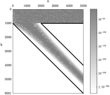
(a) Gegenbauer ($\lambda=2$)

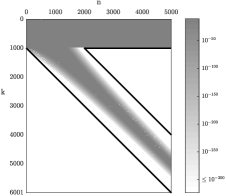
(b) Jacobi ($\alpha=2,\beta=3/2$)

Fig. 5: Entrywise error of (a) the Gegenbauer-based convolution matrix and (b) the Jacobi-based convolution matrix obtained using Algorithm 2. For both examples, $M=1000$ and $N=5000$.

5 Laguerre-based convolution matrices

If a smooth function defined on a semi-infinite domain decays to zero fast enough, it can be approximated by a series of weighted Laguerre polynomials

(50) $$L_{n}^{W}(x)=e^{-x/2}L_{n}(x),$$

where $L_{n}(x)$ is the Laguerre polynomial of degree $n$. Thus we consider the approximation of the convolution operator defined by such a function using Laguerre-based convolution matrices. We start with the following lemma which can be found in many standard texts, for example, [7, (18.17.2)].

Lemma 15 (Convolution of Laguerre polynomials).

(51) $$\int_{0}^{x}L_{m}(x-t)L_{n}(t)\mathrm{d}t=L_{m+n}(x)-L_{m+n+1}(x),$$

for $x\in[0,\infty]$.

Consider the convolution of continuous decaying functions $f(x)$ and $g(x)$ defined on $[0,\infty]$:

(52) $$V[f](g)=h(x)=\int_{0}^{x}f(x-t)g(t)\mathrm{d}t,~{}~{}~{}~{}~{}x\in[0,\infty].$$

Suppose that $f(x)$ and $g(x)$ are represented by infinite weighted Laguerre series

(53) $$f(x)=e^{-x/2}\sum_{m=0}^{\infty}a_{m}L_{m}(x)\quad\mbox{and}\quad g(x)=e^{-x/2}\sum_{n=0}^{\infty}b_{n}L_{n}(x),\qquad x\in[0,\infty],$$

and assume that the convolution

(54) $$h(x)=e^{-x/2}\sum_{k=0}^{\infty}c_{k}L_{k}(x),\qquad x\in[0,\infty],$$

so that $\underline{c}=R^{L}\underline{b}$, where $R^{L}$ is the Laguerre convolution matrices generated by $\underline{a}$. By Lemma 15, the entries of $R^{L}$ are explicitly known.

Theorem 16 (Construction of $R^{L}$).

The matrix approximation of convolution operator $V[f]$ in Laguerre space is the difference of two lower triangular Toeplitz matrices, where the second one is obtained by adding one row of zeros on the top of the first:

(55) $$R^{L}=\begin{pmatrix}a_{0}&0&0&0&\cdots\\[-3.99994pt] a_{1}&a_{0}&0&0&\ddots\\[-3.99994pt] a_{2}&a_{1}&a_{0}&0&\ddots\\[-3.99994pt] a_{3}&a_{2}&a_{1}&a_{0}&\ddots\\[-3.99994pt] \vdots&\ddots&\ddots&\ddots&\ddots\end{pmatrix}-\begin{pmatrix}0&0&0&0&\cdots\\[-3.99994pt] a_{0}&0&0&0&\ddots\\[-3.99994pt] a_{1}&a_{0}&0&0&\ddots\\[-3.99994pt] a_{2}&a_{1}&a_{0}&0&\ddots\\[-3.99994pt] \vdots&\ddots&\ddots&\ddots&\ddots\end{pmatrix}.$$

When $f(x)$ and $g(x)$ are approximated by finite weighted Laguerre series, the convolution matrix $R^{L}$ becomes a banded lower-triangular Toeplitz matrix, as shown in Figure 6(a) and the Toeplitz structure allows the fast application of $R^{L}$ to $\underline{b}$ with the aid of FFT.

Example 6: We consider the convolution of

$$f(x)=\frac{1}{2}x^{2}e^{-x}~{}\mbox{ and }~{}g(x)=-\frac{1}{3}\left(\cos\frac{\sqrt{3}}{2}x+\sqrt{3}\sin\frac{\sqrt{3}}{2}x\right)e^{-3x/2},\quad x\in[0,\infty],$$

which are the functions from Example 4, only except that the constant $1/3$ is removed from the original $g(x)$ so that both the functions decay to zero at infinity. These two functions can be approximated by weighted Laguerre series of degree $2$ and $54$, respectively. In Figure 6(b), the pointwise error in the computed approximant against the exact convolution

$$h(x)=(f\ast g)(x)=-\frac{1}{3}e^{-3x/2}\left[e^{x/2}\left(x^{2}-x-1\right)+\sqrt{3}\sin\left(\frac{\sqrt{3}x}{2}\right)+\cos\left(\frac{\sqrt{3}x}{2}\right)\right]$$

is shown up to $x=10^{4}$ and the maximum error throughout $[0,\infty]$ is approximately $4.4\times 10^{-15}$, occurring at about $x=2.9$.

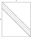
(a)         

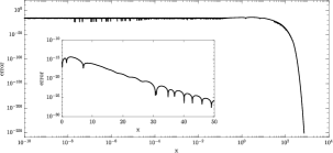
(b)

Fig. 6: (a) A schematic of Laguerre convolution matrices, where we use stripes to indicate the Toeplitz structure. Outside the striped region, all entries are exactly zero. (b) Absolute error in the computed approximation to the convolution, where the inset is a close-up for $[0,50]$.

6 Closing remarks

While we have focused exclusively on the left-sided convolution operator, with a few minor changes the framework we have presented can be extended to the right-sided convolution operator

(56) $$V[f](g)=\int_{x-1}^{1}f(x-t)g(t)\mathrm{d}t,~{}~{}~{}~{}~{}x\in[0,2],$$

with $f(x)$ and $g(x)$ compactly supported on $[-1,1]$ and the right-sided convolution matrices also enjoy similar recurrences and symmetric properties.

In Example 4, we have shown how convolution matrices can be employed to solve convolution integral equations. With the almost-banded structure of the convolution matrices, a fast spectral method can be developed based on the framework of infinite-dimensional linear algebra [20] for solving convolution integro-differential equations of Volterra type:

(57) $$\sum_{j=0}^{J}b^{j}(x)\frac{\mathrm{d}^{j}u(x)}{\mathrm{d}x^{j}}+b^{J+1}(x)\int_{a}^{x}K(x-t)u(t)\mathrm{d}t=s(x),$$

where $b^{j}(x)$ for $0\leqslant j\leqslant J+1$ are smooth functions on $[-1,1]$ and the convolution kernel $K(x-t)$ is smooth or weakly singular. We will report this line of research in a future work.

References

- [1] K. Atkinson, The Numerical Solution of Integral Equations of the Second Kind, Cambridge University Press, 1997.
- [2] J. L. Aurentz and L. N. Trefethen, Chopping a Chebyshev series, ACM Trans. Math. Softw., 43 (2017), pp. 33:1–33:21.
- [3] Z. Battles and L. N. Trefethen, An extension of MATLAB to continuous functions and operators, SIAM J. Sci. Comput., 25 (2004), pp. 1743–1770.
- [4] H. Brunner and P. J. van der Houwen, The Numerical Solution of Volterra Equations, Elsevier, 1986.
- [5] S. B. Damelin and W. Miller Jr, The Mathematics of Signal Processing, Cambridge University Press, 2012.
- [6] A. Dixit, L. Jiu, V. H. Moll, and C. Vignat, The finite Fourier transform of classical polynomials, Journal of the Australian Mathematical Society, 98 (2015), pp. 145–160.
- [7] NIST Digital Library of Mathematical Functions. http://dlmf.nist.gov/, Release 1.0.18 of 2018-03-27. F. W. J. Olver, A. B. Olde Daalhuis, D. W. Lozier, B. I. Schneider, R. F. Boisvert, C. W. Clark, B. R. Miller and B. V. Saunders, eds.
- [8] T. A. Driscoll, N. Hale, and L. N. Trefethen, eds., Chebfun Guide, Pafnuty Publications, Oxford, 2014.
- [9] D. G. Duffy, Green’s Functions with Applications, CRC Press, 2015.
- [10] W. Feller, On the integral equation of renewal theory, Ann. Math. Statist., 12 (1941), pp. 243–267.
- [11] D. Forsyth and J. Ponce, Computer Vision: A Modern Approach, Prentice Hall, 2011.
- [12] T. Hagstrom, Radiation boundary conditions for the numerical simulation of waves, Acta Numerica, 8 (1999), pp. 47–106.
- [13] N. Hale and A. Townsend, An algorithm for the convolution of Legendre series, SIAM J. Sci. Comput., 36 (2014), pp. A1207–A1220.
- [14] R. Hilfer, Applications of Fractional Calculus in Physics, World Scientific, 2000.
- [15] R. V. Hogg, J. McKean, and A. T. Craig, Introduction to Mathematical Statistics, Pearson Education, 7th ed., 2013.
- [16] IEEE, 754–2008 IEEE standard for floating-point arithmetic, 2008.
- [17] P. Linz, Analytical and Numerical Methods for Volterra Equations, SIAM, 1985.
- [18] A. F. Loureiro and K. Xu, Volterra-type convolution of classical polynomials, in prep.
- [19] J. C. Mason and D. C. Handscomb, Chebyshev Polynomials, CRC Press, Boca Raton, 2003.
- [20] S. Olver and A. Townsend, A fast and well-conditioned spectral method, SIAM Rev., (2013), pp. 462–489.
- [21] J. Shen, T. Tang, and L.-L. Wang, Spectral Methods: Algorithms, Analysis and Applications, Springer, 2011.
- [22] E. D. Sontag, Mathematical Control Theory: Deterministic Finite Dimensional Systems, Springer, 2013.
- [23] I. Stakgold and M. J. Holst, Green’s Functions and Boundary Value Problems, John Wiley & Sons, 2011.
- [24] G. W. Stewart, Afternotes goes to graduate school, SIAM, Philadelphia, PA, 1998.
- [25] G. Szegő, Orthogonal Polynomials, American Mathematical Society, 1939.
- [26] L. N. Trefethen, Approximation Theory and Approximation Practice, SIAM, Philadelphia, 2013.
- [27] C. Wagner, T. Hüttl, and P. Sagaut, Large-Eddy Simulation for Acoustics, Cambridge University Press, 2007.
- [28] H. Wang, On the optimal estimates and comparison of Gegenbauer expansion coefficients, SIAM J. Numer. Anal., 54 (2016), pp. 1557–1581.
- [29] H. Wang and S. Xiang, On the convergence rates of Legendre approximation, Math. Comput., 81 (2012), pp. 861–877.
- [30] K. Xu, A. P. Austin, and K. Wei, A fast algorithm for the convolution of functions with compact support using Fourier extensions, SIAM J. Sci. Comput., 39 (2017), pp. A3089–A3106.
- [31] X. Zhao, L.-L. Wang, and Z. Xie, Sharp error bounds for Jacobi expansions and Gegenbauer–Gauss quadrature of analytic functions, SIAM J. Numer. Anal., 51 (2013), pp. 1443–1469.