Bayesian Bandwidth Test and Selection for High-dimensional Banded Precision Matrices

Kyoungjae Lee Department of Applied and Computational Mathematics and Statistics, The University of Notre Dame Lizhen Lin Department of Applied and Computational Mathematics and Statistics, The University of Notre Dame
Abstract

Assuming a banded structure is one of the common practice in the estimation of high-dimensional precision matrix. In this case, estimating the bandwidth of the precision matrix is a crucial initial step for subsequent analysis. Although there exist some consistent frequentist tests for the bandwidth parameter, bandwidth selection consistency for precision matrices has not been established in a Bayesian framework. In this paper, we propose a prior distribution tailored to the bandwidth estimation of high-dimensional precision matrices. The banded structure is imposed via the Cholesky factor from the modified Cholesky decomposition. We establish the strong model selection consistency for the bandwidth as well as the consistency of the Bayes factor. The convergence rates for Bayes factors under both the null and alternative hypotheses are derived which yield similar order of rates. As a by-product, we also proposed an estimation procedure for the Cholesky factors yielding an almost optimal order of convergence rates. Two-sample bandwidth test is also considered, and it turns out that our method is able to consistently detect the equality of bandwidths between two precision matrices. The simulation study confirms that our method in general outperforms the existing frequentist and Bayesian methods.

Key words: Precision matrix; Bandwidth selection; Cholesky factor; Convergence rates of Bayes factor.

1 Introduction

Estimating a large covariance or precision matrix is a challenging task in both frequentist and Bayesian frameworks. When the number of variables $p$ is larger than the sample size $n$, the traditional sample covariance matrix does not provide a consistent estimate of the true covariance matrix (Johnstone and Lu, 2009), and the inverse Wishart prior leads to the posterior inconsistency (Lee and Lee, 2018). To overcome this issue, various restricted classes of matrices have been investigated such as the bandable matrices (Bickel and Levina, 2008; Cai et al., 2010; Hu and Negahban, 2017; Banerjee and Ghosal, 2014; Lee and Lee, 2017), sparse matrices (Cai and Zhou, 2012a; Banerjee and Ghosal, 2015; Xiang et al., 2015; Cao et al., 2017) and low-dimensional structural matrices (Fan et al., 2008; Cai et al., 2015; Pati et al., 2014; Gao and Zhou, 2015). In this paper, we focus on banded precision matrices, where the banded structure is encoded via the Cholesky factor of the precision matrix. We are in particular interested in the estimation of the bandwidth parameter and construction of Bayesian bandwidth tests for one or two banded precision matrices. Inference of the bandwidth is of great importance for detecting the dependence structure of the ordered data. Moreover, it is a crucial initial step for subsequent analysis such as linear or quadratic discriminant analysis.

Bandwidth selection of the high-dimensional precision matrices has received increasing attention in recent years. An et al. (2014) proposed a test for bandwidth selection, which is asymptotically normal under the null hypothesis and has a power tending to one. Based on the proposed test statistics, they constructed a backward procedure to detect the true bandwidth by controlling the familywise errors. Cheng et al. (2017) suggested a bandwidth test without assuming any specific parametric distribution for the data and obtained a result similar to that of An et al. (2014).

In the Bayesian literature, Banerjee and Ghosal (2014) studied the estimation of bandable precision matrices which include the banded precision matrix as a special case. They derived the posterior convergence rate of the precision matrix under the $G$-Wishart prior (Roverato, 2000). Lee and Lee (2017) considered a similar class to that of Banerjee and Ghosal (2014), but assumed bandable Cholesky factors instead of bandable precision matrices. They showed the posterior convergence rates of the precision matrix as well as the minimax lower bounds. In both works, posterior convergence rates were obtained for a given (fixed) bandwidth, and the posterior mode was suggested as a bandwidth estimator in practice. However, no theoretical guarantee is provided for such estimators. Further, no Bayesian bandwidth test exists for one- or two-sample problems.

This gap in the literature motivates us to investigate theoretical properties related to the general problem of bandwidth test and selection, and propose estimators or tests with theoretical guarantees. In this paper, we use the modified Cholesky decomposition of the precision matrix and assume banded Cholesky factors. The induced precision matrix also has banded structure. The key difference from Lee and Lee (2017) is on the choice of prior distributions which will be introduced in Section 2.3. In addition, we focus on bandwidth selection and tests, while Lee and Lee (2017) mainly studied the convergence rates of the precision matrix for a given or fixed bandwidth.

There are two main contributions of this paper. First, we suggest a Bayesian procedure for banded precision matrices and prove the bandwidth selection consistency (Theorem 3.1) and consistency of the Bayes factor (Theorem 3.2). To the best of our knowledge, our work is the first that has established the bandwidth selection consistency for precision matrices under a Bayesian framework, which implies that the marginal posterior probability for the true bandwidth tends to one as $n\to\infty$.Cao et al. (2017) proved strong model selection consistency for the sparse directed acyclic graph models, but their method is not applicable to the bandwidth selection problem since it is not adaptive to the unknown sparsity. Second, we also prove the consistency of the Bayes factor for two-sample bandwidth testing problem (Theorem 3.3) and derived the convergence rates of the Bayes factor under both the null and alternative hypotheses. Our method is able to consistently detect the equality of bandwidths between two different precision matrices. To the best of our knowledge, this is also the first consistent two-sample bandwidth test result in both frequentist and Bayesian literature. The existing literature (frequentist) focused only on the one-sample bandwidth testing (An et al., 2014; Cheng et al., 2017).

The rest of the paper is organized as follows. Section 2 introduces the notations, model, priors and assumptions used. Section 3 describes main results of this paper: bandwidth selection consistency and convergence rates of one- and two-sample bandwidth tests. Simulation study and real data analysis are presented in Section 4 to show the practical performance of the proposed method. In Section 5, concluding remarks and topics for the future work are given. The appendix includes a result on the nearly optimal estimation of the Cholesky factors, and proofs of main results.

2 Preliminaries

2.1 Notations

For any real numbers $a$ and $b$, we denote $a\wedge b$ and $a\vee b$ as the minimum and maximum of $a$ and $b$, respectively. For any sequences $a_{n}$ and $b_{n}$, we denote $a_{n}=o(b_{n})$ if $a_{n}/b_{n}\to 0$ as $n\to\infty$. We write $a_{n}\lesssim b_{n}$, or $a_{n}=O(b_{n})$, if there exists an universal constant $C>0$ such that $a_{n}\leq Cb_{n}$ for any $n$. We define vector $\ell_{2}$- and $\ell_{\infty}$-norms as $\|a\|_{2}=(\sum_{j=1}^{p}a_{j}^{2})^{1/2}$ and $\|a\|_{\infty}=\max_{1\leq j\leq p}|a_{j}|$ for any $a=(a_{1},\ldots,a_{p})^{T}\in\mathbb{R}^{p}$. For a matrix $A$, the matrix $\ell_{\infty}$-norm is defined as $\|A\|_{\infty}=\sup_{\|x\|_{\infty}=1}\|Ax\|_{\infty}$. We denote $\lambda_{\min}(A)$ and $\lambda_{\max}(A)$ as the minimum and maximum eigenvalues of $A$, respectively.

2.2 Gaussian Models

We consider a Gaussian model

$\displaystyle X_{1},\ldots,X_{n}\mid\Omega_{n}$ $\displaystyle\overset{i.i.d.}{\sim}$ $\displaystyle N_{p}(0,\Omega_{n}^{-1}),$ (1)

where $\Omega_{n}=\Sigma_{n}^{-1}$ is a $p\times p$ precision matrix and $X_{i}=(X_{i1},\ldots,X_{ip})^{T}\in\mathbb{R}^{p}$ for all $i=1,\ldots,n$. For any positive definite matrix $\Omega_{n}$, there exist unique lower triangular matrix $A_{n}=(a_{jl})$ and diagonal matrix $D_{n}=diag(d_{j})$ such that

$\displaystyle\Omega_{n}$ $\displaystyle=$ $\displaystyle(I_{p}-A_{n})^{T}D_{n}^{-1}(I_{p}-A_{n}),$ (2)

where $a_{jj}=0$ and $d_{j}>0$ for all $j=1,\ldots,p$, by the modified Cholesky decomposition (MCD). We call $A_{n}$ the Cholesky factor. Define $k$ as the bandwidth of a matrix if the off-diagonal elements of the matrix farther than $k$ from the diagonal are all zero. If the bandwidth of the Cholesky factor is $k$, model (1) can be represented as

$\displaystyle\begin{split}{X}_{i1}\mid d_{1}\,\,&\overset{i.i.d.}{\sim}\,\,N(0,\,d_{1}),\\ {X}_{ij}\mid a_{j}^{(k)},d_{j},k\,\,&\overset{ind}{\sim}\,\,N\Big{(}\sum_{l=(j-k)_{1}}^{j-1}{X}_{il}a_{jl},\,d_{j}\Big{)},~{}~{}j=2,\ldots,p\end{split}$ (3)

for all $i=1,\ldots,n$, where $a_{j}^{(k)}=(a_{jl})_{(j-k)_{1}\leq l\leq j-1}\in\mathbb{R}^{k_{j}}$, $(j-k)_{1}=1\vee(j-k)$ and $k_{j}=k\wedge(j-1)$. The above representation enables us to adopt priors and techniques in the linear regression literature.

We are interested in the consistent estimation and hypothesis test of the bandwidth $k$ of the precision matrix. From the decomposition (2), the bandwidth of $A_{n}$ is $k$ if and only if the bandwidth of $\Omega_{n}$ is $k$. Thus, we can infer the bandwidth of the precision matrix by inferring that of the Cholesky factor.

2.3 Prior Distribution

Let $\tilde{X}_{j}\in\mathbb{R}^{n}$ and ${{\bf X}_{j(k)}}\in\mathbb{R}^{n\times k_{j}}$ be sub-matrices consisting of $j$th and $(j-k)_{1},\ldots,(j-1)$th columns of ${\bf X}_{n}=(X_{1}^{T},\ldots,X_{n}^{T})^{T}\in\mathbb{R}^{n\times p}$, respectively. We suggest the following prior distribution

$\displaystyle a_{j}^{(k)}\mid d_{j},k$ $\displaystyle\overset{ind}{\sim}$ $\displaystyle N_{k_{j}}\left(\widehat{a}_{j}^{(k)},\,\,\frac{d_{j}}{\gamma}\big{(}{{\bf X}_{j(k)}}^{T}{{\bf X}_{j(k)}}\big{)}^{-1}\right),~{}~{}j=2,\ldots,p,$ (4)
$\displaystyle\pi(d_{j})$ $\displaystyle\overset{i.i.d.}{\propto}$ $\displaystyle d_{j}^{\tau n/2-1},~{}~{}j=1,\ldots,p,$ (5)
$\displaystyle k$ $\displaystyle\sim$ $\displaystyle\pi(k),~{}~{}k=0,1,\ldots,R_{n}$ (6)

for some positive constants $\gamma,\tau$ and positive sequence $R_{n}$, where $\widehat{a}_{j}^{(k)}=({{\bf X}_{j(k)}}^{T}{{\bf X}_{j(k)}})^{-1}{{\bf X}_{j(k)}}^{T}\tilde{X}_{j}$. The conditional prior distribution for $a_{j}^{(k)}$ is a version of the Zellner’s $g$-prior (Zellner, 1986; Martin et al., 2017) in the linear regression literature. Note that model (3) is equivalent to $\tilde{X}_{j}\mid a_{j}^{(k)},d_{j},k\sim N_{n}\big{(}{\bf X}_{j(k)}a_{j}^{(k)},d_{j}I_{n}\big{)}$. Due to the conjugacy, it enables us to calculate the posterior distribution in a closed form up to some normalizing constant. The prior for $d_{j}$ is carefully chosen to reduce the posterior mass towards large bandwidth $k$. We emphasize here that one can use the usual non-informative prior $\pi(d_{j})\propto d_{j}^{-1}$, but necessary conditions for the main results in Section 3 should be changed. This issue will be discussed in more details in the next paragraph. We assume the prior $\pi(k)$ to have the support on $0,1,\ldots,R_{n}$. We will introduce condition (A4) for $\pi(k)$ and the hyperparameters in Section 2.4, and show that $\pi(k)\propto 1$ is enough to establish the main results in Section 3.

The priors (4)–(6) lead to the following joint posterior distribution,

$\displaystyle\begin{split}a_{j}^{(k)}\mid d_{j},k,{\bf X}_{n}\,\,&\overset{ind}{\sim}\,\,N_{k_{j}}\left(\widehat{a}_{j}^{(k)},~{}\frac{d_{j}}{1+\gamma}\big{(}{{\bf X}_{j(k)}}^{T}{{\bf X}_{j(k)}}\big{)}^{-1}\right),\quad j=2,\ldots,p,\\ d_{j}\mid k,{\bf X}_{n}\,\,&\overset{ind}{\sim}\,\,IG\left(\frac{(1-\tau)n}{2},\frac{n}{2}\widehat{d}_{j}^{(k)}\right),\quad j=1,\ldots,p,\\ \pi(k\mid{\bf X}_{n})\,\,&\propto\,\,\pi(k)\prod_{j=2}^{p}\left(1+\frac{1}{\gamma}\right)^{-\frac{k_{j}}{2}}(\widehat{d}_{j}^{(k)})^{-\frac{(1-\tau)n}{2}},\quad k=0,1,\ldots,R_{n},\end{split}$ (7)

provided that $\tau<1$, where $\widehat{d}_{j}^{(k)}=\tilde{X}_{j}^{T}(I-\tilde{P}_{jk})\tilde{X}_{j}/n$ and $\tilde{P}_{jk}={{\bf X}_{j(k)}}({{\bf X}_{j(k)}}^{T}{{\bf X}_{j(k)}})^{-1}{{\bf X}_{j(k)}}^{T}$. The marginal posterior $\pi(k\mid{\bf X}_{n})$ consists of two parts: the penalty on the model size, $\pi(k)\prod_{j=2}^{p}(1+1/\gamma)^{-k_{j}/2}$, and the estimated residual variances, $\prod_{j=2}^{p}(\widehat{d}_{j}^{(k)})^{-(1-\tau)n/2}$. Thus, priors (4) and (5) naturally impose the penalty term $\prod_{j=2}^{p}(1+1/\gamma)^{-k_{j}/2}$ for the marginal posterior $\pi(k\mid{\bf X}_{n})$.

The effect of prior $\pi(d_{j})\propto d_{j}^{\tau n/2-1}$ appears in marginal posterior for $k$. Compared with the prior $\pi(d_{j})\propto d_{j}^{-1}$, it produces the term $(\widehat{d}_{j}^{(k)})^{-(1-\tau)n/2}$ instead of $(\widehat{d}_{j}^{(k)})^{-n/2}$. Thus, it reduces the posterior mass towards large bandwidth $k$ since $\widehat{d}_{j}^{(k)}$ decreases as $k$ grows. We conjecture that, at least for our prior choice of $\pi(a_{j}^{(k)}\mid d_{j},k)$ with a constant $\gamma>0$, this power adjustment of $\widehat{d}_{j}^{(k)}$ is essential to prove the selection consistency for $k$. Suppose we use the prior $\pi(d_{j})\propto d_{j}^{-1}$. Similar to the proof of Theorem 3.1, to obtain the selection consistency, we will use the inequality

$\displaystyle\pi(k\mid{\bf X}_{n})$ $\displaystyle\leq$ $\displaystyle\frac{\pi(k\mid{\bf X}_{n})}{\pi(k_{0}\mid{\bf X}_{n})}\,=\,\frac{\pi(k)}{\pi(k_{0})}\prod_{j=2}^{p}\left(1+\frac{1}{\gamma}\right)^{-\frac{k_{j}-k_{0j}}{2}}\left(\frac{\widehat{d}_{j}^{(k)}}{\widehat{d}_{j}^{(k_{0})}}\right)^{-\frac{n}{2}},$ (8)

and show that the expectation of the right hand side term converges to zero for any $k\neq k_{0}$ as $n\to\infty$, where $k_{0}$ is the true bandwidth. Note that unless $\pi(k_{0}\mid{\bf X}_{n})$ shrinks to zero, the inequality causes only a constant multiplication. The most important task is dealing with the last term in (8), $(\widehat{d}_{j}^{(k)}/\widehat{d}_{j}^{(k_{0})})^{-n/2}$. Concentration inequalities for chi-square random variables (for examples, see Lemma 3 in Yang et al. (2016) and Lemma 4 in Shin et al. (2018)) suggest an upper bound $p^{\alpha(k_{j}-k_{0j})}$ with high probability for any $2\leq j\leq p$, $k>k_{0}$ and some constant $\alpha>0$. In this case, the hyperparameter $\gamma$ should be of order $p^{-\alpha^{\prime}}$ for some constant $\alpha^{\prime}>2\alpha$ to make the right hand side in (8) converge to zero. Then, with the choice $\gamma\asymp p^{-\alpha^{\prime}}$, condition (A2), which will be introduced in Section 2.4, should be modified by replacing $1/n$ with $(\log p)/n$ to achieve the selection consistency. In summary, the main results in this paper still hold for the prior $\pi(d_{j})\propto d_{j}^{-1}$, but it requires stronger conditions due to technical reasons. We state the results using prior (5) to emphasize that the bandwidth selection problem essentially requires weaker condition than the usual model selection problem.

  • Remark

    If we adopt the fractional likelihood (Martin et al., 2017), we can achieve the selection consistency (Theorem 3.1) with the prior $\pi(d_{j})\propto d_{j}^{-1}$ instead of (5) under similar conditions in Theorem 3.1. However, with the fractional likelihood, we cannot calculate the Bayes factor which is essential to describe the Bayesian test results in Sections 3.2 and 3.3.

  • Remark

    There are two consequences by using the data-dependent mean $\widehat{a}_{j}^{(k)}$. First, we can avoid assuming an upper bound condition for $\|{\bf X}_{j(k_{0})}a_{0,j}^{(k_{0})}\|_{2}$ or $\|a_{0,j}^{(k_{0})}\|_{2}$, where $a_{0,j}^{(k_{0})}=(a_{0,jl})_{(j-k_{0})_{1}\leq l\leq j-1}$ denotes the sub-vector of the true Cholesky factor. An upper bound condition is required if we adopt the Zellner’s $g$-prior with zero mean (Shang and Clayton, 2011), e.g., Yang et al. (2016) assumed $\|{\bf X}_{j(k_{0})}a_{0,j}^{(k_{0})}\|_{2}^{2}\leq\gamma^{-1}d_{0j}\log p$ in order to prove selection consistency for the regression coefficient vector. Second, we do not need to assume the so-called information paradox of Zellner’s $g$-prior (Liang et al., 2008), which corresponds to $\gamma=p^{-2c}$ for some $c\geq 1/2$ in our notation. In this paper, we assume $\gamma$ is a constant satisfying some conditions in Section 2.4.

2.4 Assumptions

We denote $\Omega_{0n}$ as the true precision matrix whose MCD is given by $\Omega_{0n}=(I_{p}-A_{0n})^{T}D_{0n}^{-1}(I_{p}-A_{0n})$. Let $\mathbb{P}_{0}$ and $\mathbb{E}_{0}$ be the probability measure and expectation corresponding to model (1) with $\Omega_{0n}$. For the true Cholesky factor $A_{0n}=(a_{0,jl})$, we denote $k_{0}$ as the true bandwidth. We introduce conditions (A1)–(A4) for the true precision matrix and priors (4)–(6):
(A1). Assume that $p$ increases to the infinity as $n\to\infty$. Furthermore, there exist positive sequences $\epsilon_{0n}\leq 1$ and $\zeta_{0n}\geq 1$ such that $\epsilon_{0n}\leq\lambda_{\min}(\Omega_{0n})\leq\lambda_{\max}(\Omega_{0n})\leq\zeta_{0n}$ for every $n\geq 1$ and $\zeta_{0n}\log p/\epsilon_{0n}=o(n)$.
(A2). For a given positive constant $\tau\in(0,0.4]$ in prior (5), there exists a positive constant $M_{\rm bm}$ such that for every $n\geq 1$,

$\displaystyle\min_{j,l:a_{0,jl}\neq 0}|a_{0,jl}|^{2}$ $\displaystyle\geq$ $\displaystyle\frac{10M_{\rm bm}}{\tau(1-\tau)\,n}\,\frac{\zeta_{0n}}{\epsilon_{0n}}.$

(A3). The sequence $R_{n}$ in prior (6) satisfies $k_{0}\leq R_{n}\leq\min\big{\{}n\tau\epsilon_{1}(1+\epsilon_{1})^{-1},(1-\epsilon_{2})p\big{\}}$ for some small $0<\epsilon_{1},\epsilon_{2}<1$ and all sufficiently large $n$.
(A4). For given positive constants $\gamma$ and $\tau\in(0,0.4]$ in priors (4) and (5), assume that

$\displaystyle\sum_{k>k_{0}}\frac{\pi(k)}{\pi(k_{0})}\left\{C_{\gamma,\tau}\right\}^{-(k-k_{0})\cdot(p-\frac{k+k_{0}+1}{2})}$ $\displaystyle=$ $\displaystyle o(1),$ (9)
$\displaystyle\sum_{k<k_{0}}\frac{\pi(k)}{\pi(k_{0})}\left\{C_{\gamma,M_{\rm bm}}\right\}^{(k_{0}-k)\cdot(p-\frac{k+k_{0}+1}{2})}$ $\displaystyle=$ $\displaystyle o(1),$ (10)

where $C_{\gamma,\tau}=\big{\{}(1+\gamma^{-1})\cdot\tau(1+\epsilon_{1})^{-1}\big{\}}^{1/2}$ and $C_{\gamma,M_{\rm bm}}=2\,(1+\gamma^{-1})^{1/2}\exp(-M_{\rm bm})$.

Now, let us describe the above conditions in more detail. The bounded eigenvalue condition for the true precision matrix is common in the high-dimensional precision matrix literature (Banerjee and Ghosal, 2014, 2015; Xiang et al., 2015; Ren et al., 2015). We allow that $\epsilon_{0n}\to 0$ and $\zeta_{0n}\to\infty$ as $n\to\infty$, so condition (A1) is much weaker than the condition in the above literature, which assumes $\epsilon_{0n}=\zeta_{0n}^{-1}=\epsilon_{0}$ for some small constant $\epsilon_{0}>0$. Cao et al. (2017) also allowed diverging bounds, but assumed that $\zeta_{0n}=\epsilon_{0n}^{-1}$ and $(\log p/n)^{1/2-1/(2+t)}=o(\epsilon_{0n}^{4})$ for some $t>0$. If we assume that $\zeta_{0n}=\epsilon_{0n}^{-1}$, then condition (A1) implies that $\log p/n=o(\epsilon_{0n}^{2})$, which is much weaker than the condition used in Cao et al. (2017).

Condition (A2) is called the beta-min condition. If we assume that $\epsilon_{0n}=O(1)$ and $\zeta_{0n}=O(1)$, in our model it only requires the lower bound of the nonzero elements to be of order $O(1/\sqrt{n})$. In the sparse regression coefficient literature, the lower bound of the nonzero coefficients is usually assumed to be $\sqrt{\log p/n}$ up to some constant (Castillo et al., 2015; Yang et al., 2016; Martin et al., 2017). Here, the $\sqrt{\log p}$ term can be interpreted as a price coming from the absence of information on the zero-pattern. Condition (A2) reveals the fact that, under the banded assumption, we do not need to pay this price anymore.

Condition (A3) ensures that the true bandwidth $k_{0}$ lies in the support of $\pi(k)$. Note that $k_{0}\leq(1-\epsilon_{2})p$ is not an additional condition because the support of bandwidth should be smaller than $p$. The condition $k_{0}\leq n\tau\epsilon_{1}(1+\epsilon_{1})^{-1}$ is needed for the selection consistency, which holds if we choose $R_{n}=C\vee\{n\tau\epsilon_{1}(1+\epsilon_{1})^{-1}\}$ for some large constant $C>0$. Although this is slightly stronger than the condition $k_{0}\leq n-4$ in An et al. (2014), it is much weaker than those in other works. For examples, Banerjee and Ghosal (2014) assumed $k_{0}^{5}=o(n/\log p)$ for the consistent estimation of precision matrix, and Cheng et al. (2017) assumed $k_{0}=O([n/\log p]^{1/2})$ for theoretical properties.

The equations (9) and (10) in condition (A4) guarantee $\mathbb{E}_{0}[\pi(k>k_{0}\mid{\bf X}_{n})]=o(1)$ and $\mathbb{E}_{0}[\pi(k<k_{0}\mid{\bf X}_{n})]=o(1)$, respectively. Here we give some examples for $\pi(k)$ satisfying conditions (9) and (10): if we choose

$\displaystyle\pi(k)$ $\displaystyle\propto$ $\displaystyle\xi^{k(p-\frac{k+1}{2})}$ (11)

with $C_{\gamma,\tau}^{-1}<\xi<C_{\gamma,M_{\rm bm}}^{-1}$, it satisfies the conditions. Furthermore, if we choose $\xi=1$, which leads to

$\displaystyle\pi(k)$ $\displaystyle=$ $\displaystyle\frac{1}{R_{n}+1},$ (12)

the conditions are met if $\tau>(1+\epsilon_{1})(1+\gamma^{-1})^{-1}$ and $\exp(M_{\rm bm})>2(1+\gamma^{-1})^{1/2}$.

  • Remark

    In the sparse linear regression literature, a common choice for the prior on the unknown sparsity $k$ is $\pi(k)\propto p^{-ck}$ for some constant $c>0$. See Castillo et al. (2015), Yang et al. (2016) and Martin et al. (2017). If we adopt this type of the prior into the bandwidth selection problem, a naive approach is using $\pi(k)\propto p^{-ck}$ for each row of the Cholesky factor: it results in $\pi(k)\propto p^{-ck(p-k)}$. To obtain the strong model selection consistency, in this case, $M_{\rm bm}$ in condition (A2) has to be $M_{\rm bm}=M_{\rm bm}^{\prime}\,\log p$ for some constant $M_{\rm bm}^{\prime}>0$. Thus, it unnecessarily requires stronger beta-min condition, which can be avoided by using $\pi(k)$ like (11) or (12).

3 Main Results

3.1 Bandwidth Selection Consistency

When there is a natural ordering in the data set, estimating the bandwidth of the precision matrix is important for detecting the dependence structure. It is a crucial first step for the subsequent analysis. In this subsection, we show the bandwidth selection consistency of the proposed prior. Theorem 3.1 states that the posterior distribution puts a mass tending to one at the true bandwidth $k_{0}$. Thus, we can detect the true bandwidth using the marginal posterior distribution for the bandwidth $k$. We call this property the bandwidth selection consistency.

Theorem 3.1

Consider model (1) and priors (4)–(6). If conditions (A1)–(A4) are satisfied, then we have

$\displaystyle\mathbb{E}_{0}\Big{[}\pi\big{(}k\neq k_{0}\mid{\bf X}_{n}\big{)}\Big{]}$ $\displaystyle=$ $\displaystyle o(1).$

Informed readers might be aware of the recent work of Cao et al. (2017) considering the selection of sparse Cholesky factors. It should be noted that their method is not applicable to the bandwidth selection problem. The key issue is that their method is not adaptive to the unknown sparsity corresponding to the true bandwidth $k_{0}$ in this paper: to obtain the selection consistency, the choice of hyperparameter should depend on $k_{0}$, which is unknown and of interest. Furthermore, they required stronger conditions in terms of dimensionality $p$, true sparsity $k_{0}$, eigenvalues of the true precision matrix and beta-min for the strong model selection consistency.

  • Remark

    The bandwidth selection result does not necessarily imply the consistency of the Bayes factor. Note that prior (4), $\pi(d_{j})\propto d_{j}^{-1}$ and

    $\displaystyle\pi(k)$ $\displaystyle\propto$ $\displaystyle\prod_{j=2}^{p}\big{(}\widehat{d}_{j}^{(k)}\big{)}^{\frac{\tau n}{2}},$ (13)

    and priors (4), (5) and $\pi(k)\propto 1$ lead to the same marginal posterior for $k$. Thus, the above priors also achieve the bandwidth selection consistency in Theorem 3.1. However, (13) might be inappropriate when the Bayes factor is of interest, because the ratio of normalizing terms induced by prior (13) ($C_{0}$ and $C_{1}$ in (14)) have a non-ignorable effect on the Bayes factor.

3.2 Consistency of One-Sample Bandwidth Test

In this subsection, we focus on constructing a Bayesian bandwidth test for the testing problem $H_{0}:k\leq k^{\star}$ versus $H_{1}:k>k^{\star}$ for some given $k^{\star}$. A Bayesian hypothesis test is based on the Bayes factor $B_{10}({\bf X}_{n})$ defined by the ratio of marginal likelihoods,

$\displaystyle B_{10}({\bf X}_{n})$ $\displaystyle=$ $\displaystyle\frac{p({\bf X}_{n}\mid H_{1})}{p({\bf X}_{n}\mid H_{0})}.$

We are interested in the consistency of the Bayes factor which is one of the most important asymptotic properties of the Bayes factor (Dass and Lee, 2004). A Bayes factor is said to be consistent if $B_{10}({\bf X}_{n})$ converges to zero in probability under the true null hypothesis $H_{0}$ and $B_{10}({\bf X}_{n})^{-1}$ converges to zero in probability under the true alternative hypothesis $H_{1}$.

Although the Bayes factor plays a crucial role in the Bayesian variable selection, its asymptotic behaviors in the high-dimensional setting are not well-understood (Moreno et al., 2010). Few works studied the consistency of the Bayes factor in the high-dimensional settings (Moreno et al., 2010; Wang and Sun, 2014; Wang et al., 2016), which only focused on the pairwise consistency of the Bayes factor. They considered the testing problem $H_{0}:k=k^{(0)}$ versus $H_{1}:k=k^{(1)}$ for any $k^{(0)}<k^{(1)}$, where $k$ is the number of nonzero elements of the linear regression coefficient. Note that a Bayes factor is said to be pairwise consistent if the Bayes factor $B_{10}({\bf X}_{n})$ is consistent for any pair of simple hypotheses $H_{0}$ and $H_{1}$.

We focus on the composite hypotheses $H_{0}:k\leq k^{\star}$ and $H_{1}:k>k^{\star}$ rather than simple hypotheses. To conduct a Bayesian hypothesis test, prior distributions for both hypotheses should be determined. Denote the prior under the hypothesis $H_{i}$ as $\pi_{i}(A_{n},D_{n},k)$ for $i=0,1$. Since the difference between two hypotheses comes only from the bandwidth, we will use the same conditional priors for $A_{n}$ and $D_{n}$ given $k$, i.e. $\pi_{i}(A_{n},D_{n},k)=\pi_{i}(k)\,\pi(A_{n},D_{n}\mid k)$ for $i=0,1$, where $\pi(A_{n},D_{n}\mid k)$ is chosen as (4) and (5). We suggest using priors $\pi_{0}(k)$ and $\pi_{1}(k)$ such that

$$\begin{split}\pi_{0}(k)&=C_{0}^{-1}\pi(k),\quad k=0,1,\ldots,k^{\star},\\ \pi_{1}(k)&=C_{1}^{-1}\pi(k),\quad k=k^{\star}+1,\ldots,R_{n},\end{split}$$ (14)

where $C_{0}=\sum_{k=0}^{k^{\star}}\pi(k)$ and $C_{1}=\sum_{k=k^{\star}+1}^{R_{n}}\pi(k)$. Then, the Bayes factor has the following analytic form,

$\displaystyle B_{10}({\bf X}_{n})$ $\displaystyle=$ $\displaystyle\frac{\sum_{k>k^{\star}}\int p({\bf X}_{n}\mid\Omega_{n},k)\pi(\Omega_{n}\mid k)\pi_{1}(k)d\Omega_{n}}{\sum_{k\leq k^{\star}}\int p({\bf X}_{n}\mid\Omega_{n},k)\pi(\Omega_{n}\mid k)\pi_{0}(k)d\Omega_{n}}$
$\displaystyle=$ $\displaystyle\frac{\pi(k>k^{\star}\mid{\bf X}_{n})}{\pi(k\leq k^{\star}\mid{\bf X}_{n})}\times\frac{C_{0}}{C_{1}},$

where the marginal posterior $\pi(k\mid{\bf X}_{n})$ is given in (7) up to some normalizing constant. Note that, the Bayes factor can be defined because both hypotheses have the same improper priors on $D_{n}$. We will show that the Bayes factor is consistent for any composite hypotheses $H_{0}:k\leq k^{\star}$ and $H_{1}:k>k^{\star}$, which is generally stronger than the pairwise consistency of the Bayes factor. If we assume that $\pi_{1}(k)/\pi_{0}(k^{\prime})=O(1)$ for any $k$ and $k^{\prime}$, then one can see that the consistency of the Bayes factor for hypotheses $H_{0}:k\leq k^{\star}$ and $H_{1}:k>k^{\star}$ for any $k^{\star}$ implies the pairwise consistency of the Bayes factor for any pair of simple hypotheses $H_{0}:k=k^{(0)}$ and $H_{1}:k=k^{(1)}$ for $k^{(0)}<k^{(1)}$.

For given positive constants $M_{\rm bm}$, $\gamma$ and $\tau\in(0,0.4]$ and integers $R_{n}$, $k_{0}$ and $k^{\star}$, define

$\displaystyle T_{n,H_{0},k_{0},k^{\star}}$ $\displaystyle=$ $\displaystyle k^{\star}\cdot\left\{C_{\gamma,\tau}^{-1}\right\}^{(k^{\star}+1-k_{0})\cdot(p-\frac{R_{n}+k_{0}+1}{2})},$
$\displaystyle T_{n,H_{1},k_{0},k^{\star}}$ $\displaystyle=$ $\displaystyle(R_{n}-k^{\star})\cdot\left\{C_{\gamma,M_{\rm bm}}\right\}^{(k_{0}-k^{\star})\cdot(p-\frac{k^{\star}+k_{0}+1}{2})},$

where $C_{\gamma,\tau}$ and $C_{\gamma,M_{\rm bm}}$ are defined in condition (A4). Theorem 3.2 shows the convergence rates of Bayes factors under each hypothesis. It turns out that $\pi(k)=1/(R_{n}+1)$ is sufficient for the consistency of the Bayes factor.

Theorem 3.2

Consider model (1) and hypothesis testing problem $H_{0}:k\leq k^{\star}$ versus $H_{1}:k>k^{\star}$. Assume priors (4) and (5) for $\pi(A_{n},D_{n}\mid k)$ and the bandwidth priors in (14) with $\pi(k)=1/(R_{n}+1)$. If conditions (A1)–(A3) hold, $\tau>\gamma(1+\epsilon_{1})/(1+\gamma)$ and $\exp(M_{\rm bm})>2\{(1+\gamma)/\gamma\}^{1/2}$, then the Bayes factor $B_{10}({\bf X}_{n})$ is consistent under $\mathbb{P}_{0}$. Moreover, under $H_{0}:k\leq k^{\star}$, we have

$\displaystyle B_{10}({\bf X}_{n})$ $\displaystyle=$ $\displaystyle O_{p}\big{(}T_{n,H_{0},k_{0},k^{\star}}\big{)},$

and under $H_{1}:k>k^{\star}$,

$\displaystyle B_{10}({\bf X}_{n})^{-1}$ $\displaystyle=$ $\displaystyle O_{p}(T_{n,H_{1},k_{0},k^{\star}}).$
  • Remark

    By choosing the prior $\pi(k)=1/(R_{n}+1)$, it implies that $C_{\gamma,\tau}^{-1}$ and $C_{\gamma,M_{\rm bm}}$ are strictly smaller than $1$ by (11). Since we assume that $p\to\infty$ as $n\to\infty$, one can easily check that $T_{n,H_{0},k_{0},k^{\star}}$ and $T_{n,H_{1},k_{0},k^{\star}}$ go to zero as $n\to\infty$ under $H_{0}:k\leq k^{\star}$ and $H_{1}:k>k^{\star}$, respectively.

  • Remark

    Note that if we use prior (11) with $\xi\neq 1$, the effect of the prior, $C_{0}/C_{1}$, can dominate the posterior ratio, $\pi(k>k^{\star}\mid{\bf X}_{n})/\pi(k\leq k^{\star}\mid{\bf X}_{n})$ in the Bayes factor. Because the prior knowledge on the bandwidth is usually not sufficient, it is clearly undesirable. Moreover, the direction of effect is the opposite of the prior knowledge.

An et al. (2014) and Cheng et al. (2017) developed frequentist bandwidth tests for the hypotheses $H_{0}:k\leq k^{\star}$ versus $H_{1}:k>k^{\star}$ and showed that their test statistic is asymptotically normal under the null and has a power converging to one as $n\wedge p\to\infty$. Compared with the result in Theorem 3.2, Cheng et al. (2017) required the upper bound $k_{0}=O([n/\log p]^{1/2})$ for the true bandwidth $k_{0}$, which is much stronger than our condition (A3). An et al. (2014) allowed $k_{0}\leq n-4$, but assumed that the partial correlation coefficient between $X_{ij}$ and $X_{i,j-k_{0}}$ given $X_{i,j-k_{0}+1},\ldots,X_{i,j-1}$ is of order $o(n^{-1})$. It implies that $\max_{j}|a_{0,jj-k_{0}}|$ converges to zero at some rate. Thus, the nonzero elements $a_{0,jj-k_{0}}$, $j=k_{0}+1,\ldots,p$ should converge to zero, which is somewhat unnatural.

Johnson and Rossell (2010, 2012) and Rossell and Rubio (2017) pointed out that the use of local alternative prior leads to imbalanced convergence rates for the Bayes factors, and showed that this issue can be avoided by using non-local alternative priors. However, interestingly, convergence rates for the Bayes factors in Theorem 3.2 yield similar order of rates under both hypotheses without using a non-local prior. Roughly speaking, the imbalance issue can be ameliorated by introducing the beta-min condition (Condition (A2)). To simplify the situation, consider the model

$\displaystyle Y$ $\displaystyle=$ $\displaystyle X\beta^{(k)}+\epsilon,$

where $Y=(Y_{1},\ldots,Y_{n})^{T}$, $X\in\mathbb{R}^{n\times p}$, $\beta^{(k)}=(\beta_{1},\ldots,\beta_{k},0,\ldots,0)^{T}\in\mathbb{R}^{p}$, $\epsilon=(\epsilon_{1},\ldots,\epsilon_{n})^{T}$ and $\epsilon_{i}\overset{i.i.d.}{\sim}N(0,\sigma^{2})$. Suppose priors (4) and (5) are imposed on $(\beta_{1},\ldots,\beta_{k})^{T}$ and $\sigma^{2}$ given $k$. Consider hypotheses $H_{0}:k=k_{1}$ and $H_{1}:k=k_{2}$, where $k_{1}<k_{2}$, and assume that the eigenvalues of $X_{(1:k_{2})}$ are bounded and $k_{2}-k_{1}\to\infty$ as $n\to\infty$ for simplicity. Note that the prior for $\beta^{(k_{2})}$ is a local alternative prior because $\pi(\beta^{(k_{2})}\mid\sigma^{2})>c$ on $\{\beta^{(k_{2})}\in\mathbb{R}^{k_{2}}:\beta^{(k_{2})}=(\beta_{1},\ldots,\beta_{k_{1}},0,\ldots,0)^{T}\}$ for some constant $c>0$. If $H_{0}$ is true, $B_{10}(Y)$ decreases at rate $O_{p}(e^{-c_{0}(k_{2}-k_{1})})$ for some constant $c_{0}>0$ based on techniques in the proof of Theorem 3.1. On the other hand, if $H_{1}$ is true, $B_{10}(Y)^{-1}$ decreases exponentially with $n(k_{2}-k_{1})\beta_{\rm min}^{2}$, where $\beta_{\rm min}$ is the lower bound for the absolute of nonzero elements of $\beta_{0}^{(k_{2})}$. Johnson and Rossell (2010, 2012) and Rossell and Rubio (2017) assumed that $\beta_{\rm min}^{2}>c_{1}$ for some constant $c_{1}>0$. In that case, $B_{10}(Y)^{-1}$ decreases exponentially with $n(k_{2}-k_{1})c_{1}$, which causes the imbalanced convergence rates. However, if we assume $\beta_{\rm min}^{2}\geq c_{2}n^{-1}$ similar to condition (A2), $B_{10}(Y)^{-1}$ decreases at rate $O_{p}(e^{-c_{2}(k_{2}-k_{1})})$ for some constant $c_{2}>0$. Thus, convergence rates for the Bayes factors have similar order under the both hypotheses.

The above argument does not mean that the non-local priors are not useful for our problem. We note that the balanced convergence rates by using the beta-min condition is different from those by using the non-local prior. The former makes the rate of $B_{10}(Y)^{-1}$ slower under $H_{1}$, while the latter makes the rate of $B_{10}(Y)$ faster under $H_{0}$. Thus, the use of non-local priors might improve the rates of convergence for $B_{10}(Y)$ under $H_{0}$ in Theorem 3.2. However, it will increase the computational burden and is unclear which rate one can achieve using the non-local prior under condition (A2), so we leave it as a future work.

3.3 Consistency of Two-Sample Bandwidth Test

Suppose we have two data sets from the models

$\displaystyle\begin{split}X_{1},\ldots,X_{n_{1}}\mid\Omega_{1n_{1}}&\overset{i.i.d.}{\sim}N_{p}(0,\Omega_{1n_{1}}^{-1}),\\ Y_{1},\ldots,Y_{n_{2}}\mid\Omega_{2n_{2}}&\overset{i.i.d.}{\sim}N_{p}(0,\Omega_{2n_{2}}^{-1}),\end{split}$ (15)

where $\Omega_{1n_{1}}=(I_{p}-A_{1n_{1}})^{T}D_{1n_{1}}^{-1}(I_{p}-A_{1n_{1}})$ and $\Omega_{2n_{2}}=(I_{p}-A_{2n_{2}})^{T}D_{2n_{2}}^{-1}(I_{p}-A_{2n_{2}})$ are the MCDs. Denote the bandwidth of $\Omega_{in_{i}}$ as $k_{i}$ for $i=1,2$. In this subsection, our interest is the test of equality between two bandwidths $k_{1}$ and $k_{2}$, the two-sample bandwidth test. We consider the hypothesis testing problem $H_{0}:k_{1}=k_{2}$ versus $H_{1}:k_{1}\neq k_{2}$ and investigate the asymptotic behavior of the Bayes factor,

$\displaystyle B_{10}({\bf X}_{n_{1}},{\bf Y}_{n_{2}})$ $\displaystyle=$ $\displaystyle\frac{p({\bf X}_{n_{1}},{\bf Y}_{n_{2}}\mid H_{1})}{p({\bf X}_{n_{1}},{\bf Y}_{n_{2}}\mid H_{0})},$

where ${\bf X}_{n_{1}}=(X_{1}^{T},\ldots,X_{n_{1}}^{T})^{T}\in\mathbb{R}^{n_{1}\times p}$ and ${\bf Y}_{n_{2}}=(Y_{1}^{T},\ldots,Y_{n_{2}}^{T})^{T}\in\mathbb{R}^{n_{2}\times p}$. Suppose that multivariate observations are collected from two populations, and a test of the equality of dependence structure is the main interest. When the dependence structure is directly related to how many previous variables influencing the current variable, two-sample bandwidth test provides a suitable answer.

Denote the priors under $H_{0}$ and $H_{1}$ as, respectively

$\displaystyle\pi_{0}\big{(}A_{1n_{1}},D_{1n_{1}},A_{2n_{2}},D_{2n_{2}}\mid k\big{)}$
$\displaystyle=$ $\displaystyle\pi\big{(}A_{1n_{1}},D_{1n_{1}}\mid k\big{)}\,\pi\big{(}A_{2n_{2}},D_{2n_{2}}\mid k\big{)}\,\pi_{0}(k),\quad k=0,1,\ldots,R_{n},$

and

$\displaystyle\pi_{1}\big{(}A_{1n_{1}},D_{1n_{1}},A_{2n_{2}},D_{2n_{2}}\mid k_{1},k_{2}\big{)}$
$\displaystyle=$ $\displaystyle\pi\big{(}A_{1n_{1}},D_{1n_{1}}\mid k_{1}\big{)}\,\pi\big{(}A_{2n_{2}},D_{2n_{2}}\mid k_{2}\big{)}\,\pi_{1}(k_{1},k_{2}),\quad 0\leq k_{1}\neq k_{2}\leq R_{n}.$

We suggest the following conditional priors $\pi(A_{1n_{1}},D_{1n_{1}}\mid k_{1})$ and $\pi(A_{2n_{2}},D_{2n_{2}}\mid k_{2})$ for any given $k_{1}$ and $k_{2}$,

$\displaystyle\begin{split}a_{1,j}^{(k_{1})}\mid d_{1,j},k_{1}\,\,&\overset{ind}{\sim}\,\,N_{k_{1j}}\Big{(}\widehat{a}_{1,j}^{(k_{1})},\frac{d_{1,j}}{\gamma}\big{(}{\bf X}_{j(k_{1})}^{T}{\bf X}_{j(k_{1})}\big{)}^{-1}\Big{)},\\ \pi(d_{1,j})\,\,&\overset{i.i.d.}{\propto}\,\,d_{1,j}^{\tau n_{1}/2-1},\\ a_{2,j}^{(k_{2})}\mid d_{2,j},k_{2}\,\,&\overset{ind}{\sim}\,\,N_{k_{2j}}\Big{(}\widehat{a}_{2,j}^{(k_{2})},\frac{d_{2,j}}{\gamma}\big{(}{\bf Y}_{j(k_{2})}^{T}{\bf Y}_{j(k_{2})}\big{)}^{-1}\Big{)},\\ \pi(d_{2,j})\,\,&\overset{i.i.d.}{\propto}\,\,d_{2,j}^{\tau n_{2}/2-1},\end{split}$ (16)

where $k_{ij}=k_{i}\wedge(j-1)$, $a_{i,j}^{(k_{i})}\in\mathbb{R}^{k_{ij}}$ is the nonzero elements in the $j$th row of $A_{in_{i}}$ and $D_{in_{i}}=diag(d_{i,j})$ for $i=1,2$. Similar to the previous notations, we denote $\widehat{a}_{1,j}^{(k_{1})}=({\bf X}_{j(k_{1})}^{T}{\bf X}_{j(k_{1})})^{-1}{\bf X}_{j(k_{1})}^{T}\tilde{X}_{j}$ and $\widehat{a}_{2,j}^{(k_{2})}=({\bf Y}_{j(k_{2})}^{T}{\bf Y}_{j(k_{2})})^{-1}{\bf Y}_{j(k_{2})}^{T}\tilde{Y}_{j}$, where ${\bf Y}_{j(k_{2})}\in\mathbb{R}^{n\times k_{2}}$ is the sub-matrix consisting of $(j-k_{2})_{1},\ldots,(j-1)$th columns of ${\bf Y}_{n}$. The priors on bandwidths are chosen as

$$\begin{split}\pi_{0}(k)&=\frac{1}{R_{n}+1},\quad k=0,1,\ldots,R_{n},\\ \pi_{1}(k_{1},k_{2})&=\frac{1}{R_{n}(R_{n}+1)},\quad 0\leq k_{1}\neq k_{2}\leq R_{n}.\end{split}$$ (17)

This choice of priors leads to an analytic form of the Bayes factor,

$\displaystyle B_{10}({\bf X}_{n_{1}},{\bf Y}_{n_{2}})$ $\displaystyle=$ $\displaystyle\frac{\sum_{k_{1}\neq k_{2}}\pi(k_{1}\mid{\bf X}_{n_{1}})\pi(k_{2}\mid{\bf Y}_{n_{2}})}{\sum_{k_{1}=k_{2}}\pi(k_{1}\mid{\bf X}_{n_{1}})\pi(k_{2}\mid{\bf Y}_{n_{2}})}\times R_{n}^{-1},$

where the marginal posterior distributions $\pi(k_{1}\mid{\bf X}_{n_{1}})$ and $\pi(k_{2}\mid{\bf Y}_{n_{2}})$ are known up to some normalizing constants similar to (7). We denote $\Omega_{0,in_{i}}$ as the true precision matrix with bandwidth $k_{0i}$ for $i=1,2$ and assume that $p$ tends to infinity as $n=n_{1}\wedge n_{2}\to\infty$. Theorem 3.3 gives a sufficient condition for the consistency of the Bayes factor $B_{10}({\bf X}_{n_{1}},{\bf Y}_{n_{2}})$ by calculating the convergence rates.

Theorem 3.3

Consider model (15) and hypotheses $H_{0}:k_{1}=k_{2}$ and $H_{1}:k_{1}\neq k_{2}$. Assume the conditional priors given bandwidths (16) and the bandwidth priors (17). If conditions (A1)–(A3) for $\Omega_{0,1n_{1}}$, $\Omega_{0,2n_{2}}$ and priors are satisfied, $\tau>\gamma(1+\epsilon_{1})/(1+\gamma)$ and $\exp(M_{\rm bm})>2\{(1+\gamma)/\gamma\}^{1/2}$, then the Bayes factor $B_{10}({\bf X}_{n_{1}},{\bf Y}_{n_{2}})$ is consistent under $\mathbb{P}_{0}$. Moreover, under $H_{0}:k_{1}=k_{2}$, we have

$\displaystyle B_{10}({\bf X}_{n_{1}},{\bf Y}_{n_{2}})$ $\displaystyle=$ $\displaystyle O_{p}\left(\frac{k_{0}}{R_{n}-k_{0}}T_{n,H_{1},k_{0},k_{0}-1}+\frac{R_{n}-k_{0}}{k_{0}}T_{n,H_{0},k_{0},k_{0}}\right),$

and under $H_{1}:k_{1}\neq k_{2}$,

$\displaystyle B_{10}({\bf X}_{n_{1}},{\bf Y}_{n_{2}})^{-1}$ $\displaystyle=$ $\displaystyle O_{p}\left(\frac{R_{n}\,k_{\min}}{R_{n}-k_{\min}}T_{n,H_{1},k_{\min},k_{\min}-1}+\frac{R_{n}(R_{n}-k_{\min})}{k_{\min}}T_{n,H_{0},k_{\min},k_{\min}}\right),$

where $k_{\min}=k_{01}\wedge k_{02}$.

As mentioned earlier, to the best of our knowledge, this is the first consistent two-sample bandwidth test result in high-dimensional settings. Frequentist testing procedures in An et al. (2014) and Cheng et al. (2017) focused only on the one-sample bandwidth test, and it is unclear whether these methods can be extended to the two-sample testing problem.

Note that the hypothesis testing problem $H_{0}:k_{1}=k_{2}$ versus $H_{1}:k_{1}\neq k_{2}$ is different from the hypothesis testing $H_{0}:\Omega_{1n_{1}}=\Omega_{2n_{2}}$ versus $H_{1}:\Omega_{1n_{1}}\neq\Omega_{2n_{2}}$ in Cai et al. (2013). The latter testing problem is called the two-sample precision (or covariance) test. The two-sample bandwidth test is weaker than the two-sample precision test, i.e. if the two-sample bandwidth test supports the null hypothesis, then one can further conduct the two-sample precision test.

4 Numerical Results

We have proved the bandwidth selection consistency and convergence rates of Bayes factors based on priors (4)–(6). In this section, we conduct simulation studies to describe the practical performance of the proposed method. Throughout the section, we use the prior $\pi(k)=1/(R_{n}+1)$.

4.1 Comparison with other Bandwidth Tests

In this subsection, we compared the performance of our method with those of other bandwidth selection procedures. Since we have bandwidth selection consistency (Theorem 3.1), we suggest using the posterior mode to estimate the true bandwidth $k_{0}$. We chose the bandwidth test of An et al. (2014) as a frequentist competitor and the bandwidth selection procedures of Banerjee and Ghosal (2014) and Lee and Lee (2017) as Bayesian competitors. Significance levels for bandwidth tests in An et al. (2014) were varied $\alpha=0.001,0.005,0.01$, but only the result with $\alpha=0.01$ are reported since they gave similar results. For Banerjee and Ghosal (2014) and Lee and Lee (2017), we used the prior $\pi(k)\propto\exp(-k^{4})$ as they suggested. Note that these Bayesian procedures do not guarantee the bandwidth selection consistency.

To calculate the marginal posterior in (7), the hyperparameters $\gamma,\tau$ and $R_{n}$ should be determined. As a pragmatic approach, we incorporated cross-validation (CV) to select $\gamma$, and fixed $\tau=0.01$ and $R_{n}=k_{0}+10$; in our experiments, we also tried $\tau=0.01,0.02,\ldots,0.30$ and selected $\tau$ via CV, but found that $\tau=0.01$ is selected in most cases. We randomly divided the data ${\bf X}_{n}$ into two subsamples, the test set ${\bf X}_{n_{1}}^{te}$ and training set ${\bf X}_{n_{2}}^{tr}$, where $n_{1}=\lceil n/3\rceil$ and $n_{2}=n-n_{1}$. Let $\widehat{k}(\gamma)$ be the posterior mode based on ${\bf X}_{n_{2}}^{tr}$ and a given $\gamma$, and define the mean squared error (MSE)

$\displaystyle MSE(\gamma)$ $\displaystyle=$ $\displaystyle\sum_{j=1}^{p}\|\tilde{X}_{j}^{te}-{\bf X}_{j(\widehat{k}(\gamma))}^{te}\widehat{a}_{j}^{(\widehat{k}(\gamma))}\|_{2}^{2}.$

We divided the data 20 times and selected $\widehat{\gamma}$ which minimizes $20^{-1}\sum_{\nu=1}^{20}MSE_{\nu}(\gamma)$, where $MSE_{\nu}(\gamma)$ is the MSE from the $\nu$th subsampling. Depending on the purpose of the analysis, other criteria besides MSE can be adopted.

The data sets were generated from $N_{p}(0,\Omega_{0n}^{-1})$, where $\Omega_{0n}=(I_{p}-A_{0n})^{T}D_{0n}^{-1}(I_{p}-A_{0n})$. For each $j=k_{0}+1,\ldots,p$, nonzero elements in the $j$th row of the true Cholesky factor $A_{0n}$ were sampled from $Unif(A_{0,\min},A_{0,\max})$ and ordered to satisfy $a_{0,jl}\leq a_{0,jl^{\prime}}$ for any $l<l^{\prime}$. The diagonal elements of $D_{0n}$ were generated from $Unif(5,10)$. To investigate performance in various settings, the values of $n,p,k_{0},A_{0,\min}$ and $A_{0,\max}$ were varied. The simulation results, based on 50 simulated data sets for each setting, are reported in Table 1 and Figure 1. We denoted the proposed method in this paper as BBS, the Bayesian Bandwidth Selector.

Table 1: The summary statistics for each setting are represented, where $k_{0}=5$ and $[A_{0,\min},A_{0,\max}]=[0.1,0.1]$. BBS: the proposed method in this paper. LL: bandwidth selection procedure of Lee and Lee (2017). BG: bandwidth selection procedure of Banerjee and Ghosal (2014). BA1 and BA2: algorithms 1 and 2 in An et al. (2014), respectively.
$\big{(}\,\widehat{p}_{0},\,\,\widehat{k}_{0}\,\big{)}$
$(n=70,p=100)$ $(n=70,p=200)$ $(n=200,p=100)$ $(n=200,p=200)$
BBS $(0.96,\,4.94)$ $(0.98,\,4.98)$ $(1.00,\,5.00)$ $(1.00,\,5.00)$
BA1 $(0.78,\,4.84)$ $(0.96,\,5.16)$ $(0.96,\,5.06)$ $(1.00,\,5.00)$
BA2 $(0.78,\,4.84)$ $(0.98,\,5.18)$ $(0.96,\,5.06)$ $(1.00,\,5.00)$
LL $(0.00,\,1.00)$ $(0.00,\,1.00)$ $(0.00,\,1.02)$ $(0.00,1.04)$
BG $(0.00,\,1.00)$ $(0.00,\,1.00)$ $(0.00,\,1.00)$ $(0.00,1.00)$
Table 2: The summary statistics for each setting are represented, where $k_{0}=10$ and $[A_{0,\min},A_{0,\max}]=[0.1,0.2]$.
$\big{(}\,\widehat{p}_{0},\,\,\widehat{k}_{0}\,\big{)}$
$(n=70,p=100)$ $(n=70,p=200)$ $(n=200,p=100)$ $(n=200,p=200)$
BBS $(0.94,\,10.02)$ $(0.96,\,10.06)$ $(1.00,\,10.00)$ $(1.00,\,10.00)$
BA1 $(0.72,\,9.66)$ $(0.98,\,10.14)$ $(1.00,\,10.00)$ $(0.98,\,10.06)$
BA2 $(0.74,\,9.72)$ $(0.98,\,10.14)$ $(1.00,\,10.00)$ $(0.96,\,10.08)$
LL $(0.00,\,2.12)$ $(0.00,\,2.86)$ $(0.00,\,3.36)$ $(0.00,4.00)$
BG $(0.00,\,1.00)$ $(0.00,\,1.00)$ $(0.00,\,1.00)$ $(0.00,1.00)$
Refer to caption
Refer to caption
Refer to caption
Refer to caption
Figure 1: The summary plots for estimated bandwidth in various settings. The middle dot and bar represent the mean and standard error of the mean, respectively, based on 50 simulations. $[A_{0,\min},A_{0,\max}]=[0.1,0.1]$ was used for the top row, while $[A_{0,\min},A_{0,\max}]=[0.1,0.2]$ was used for the bottom row. The red dashed line is the true bandwidth.

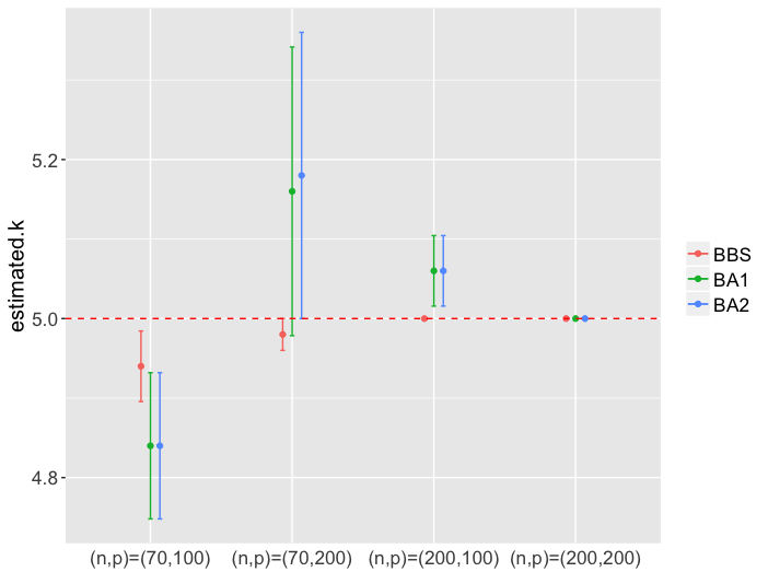
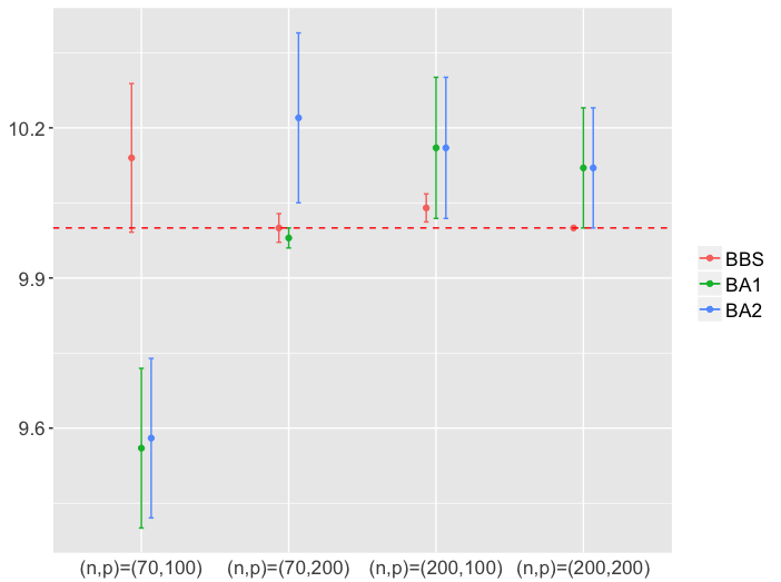
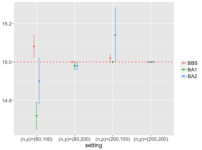
Performance of each method were evaluated by the proportion of correct detections of $k_{0}$, $\widehat{p}_{0}=\sum_{s=1}^{50}I(\hat{k}_{0}^{(s)}=k_{0})/50$, and averaged bandwidth estimate, $\widehat{k}_{0}=\sum_{s=1}^{50}\hat{k}_{0}^{(s)}/50$, where $\hat{k}_{0}^{(s)}$ is the estimated bandwidth for the $s$th data set. Our method, the BBS, consistently outperformed other competitors in most settings. The bandwidth selection procedures of An et al. (2014) worked reasonably well for large $n$ and large $p$ cases, but it seems somewhat unstable when $(n=70,p=100)$. Although Lee and Lee (2017) is slightly better than Banerjee and Ghosal (2014), both of them consistently underestimated the true bandwidth $k_{0}$. The proposed prior $\pi(k)\propto\exp(-k^{4})$ seems to be too strong to put sufficient masses near the true bandwidth $k_{0}$ especially when $k_{0}$ is not small. Figure 1 shows the bandwidth selection results of BBS and the test in An et al. (2014) to compare the performance of the two methods at a glance. As shown in Tables 1 and 2, the BBS outperformed the bandwidth tests in An et al. (2014) in most cases.

4.2 Telephone Call Center Data

We illustrate the performance of the proposed method using the telephone call center data previously analyzed by Huang et al. (2006), Bickel and Levina (2008) and An et al. (2014). The phone calls were recorded from 7:00 am until midnight from a call center of a major U.S. financial organization. The data were collected for 239 days in 2002 except holidays, weekends and days when the recording system did not work properly. The number of calls were counted for every 10 minutes, and a total of 102 intervals were obtained on each day. We denote the number of calls on the $j$th time interval of the $i$th day as $N_{ij}$ for each $i=1,\ldots,239$ and $j=1,\ldots,102$. As in Huang et al. (2006), Bickel and Levina (2008) and An et al. (2014), a transformation $X_{ij}=\sqrt{N_{ij}+1/4}$ was applied to make the data close to the random sample from normal distribution. The transformed data set was centered. For more details about the data set, see Huang et al. (2006).

We are interested in predicting the number of phone calls from the $52$nd to $102$nd time intervals using the previous counts on each day. The best linear predictor of $X_{ij}$ from $X_{i}^{j}=(X_{i1},\ldots,X_{i,j-1})^{T}$,

$\displaystyle\widehat{X}_{ij}$ $\displaystyle=$ $\displaystyle\mu_{j}+\Sigma_{(j,1:(j-1))}\big{[}\Sigma_{(1:(j-1),1:(j-1))}\big{]}^{-1}(X_{i}^{j}-\mu^{j}),$ (18)

was used to predict $X_{ij}$ for each $j=52,\ldots,102$, where $\mu_{j}=\mathbb{E}(X_{1j})$, $\mu^{j}=(\mu_{1},\ldots,\mu_{j-1})^{T}$ and $\Sigma_{S_{1},S_{2}}$ is a sub-matrix of $\Sigma$ consisting of the $S_{1}$th rows and the $S_{2}$th columns for given index sets $S_{1}$ and $S_{2}$. We used the first 205 days $(i=1,\ldots,205)$ as a training set and the last 34 days $(i=206,\ldots,239)$ as a test set. To calculate the best linear predictor (18), the unknown parameters are need to be estimated. Because it is reasonable to assume the existence of the natural (time) ordering, we plugged the estimators $\widehat{\mu}^{j}=\sum_{i=1}^{205}X_{i}^{j}/205$ and $\widehat{\Sigma}_{k}=\big{\{}(I_{p}-\widehat{A}_{nk})^{T}\widehat{D}_{nk}^{-1}(I_{p}-\widehat{A}_{nk})\big{\}}^{-1}$ into (18), where $\widehat{A}_{nk}$ and $\widehat{D}_{nk}$ are estimators based on the training set.

We applied the proposed methods in this paper, An et al. (2014) and Bickel and Levina (2008) to estimate the bandwidth $k$ using the training set, and compared the prediction errors $\text{PE}_{j}=\sum_{i=206}^{239}|\widehat{X}_{ij}-X_{ij}|/34$ for each $j=52,\ldots,102$. We defined the average of prediction errors, $\sum_{j=52}^{102}\text{PE}_{j}/51$ to illustrate the performance of estimated bandwidths. For a fair comparison, we used the same estimator $\widehat{\Sigma}_{k}$ and only chose different bandwidths depending on the selection procedure. Since the goal of the analysis is prediction, the average of prediction errors using training set was used as the criterion for CV. Based on the selected hyperparameter, our method, the BBS, gives the estimated bandwidth $\widehat{k}=5$. Algorithms 1 and 2 with $\alpha=0.01$ in An et al. (2014) determined the bandwidth as 8 and 10, respectively, and Bickel and Levina (2008) selected the bandwidth as 19 based on a resampling scheme proposed in their paper. The average of prediction errors were $0.5347,0.5474,0.5568$ and $0.5609$ at bandwidth $k=5$, $8$, $10$ and $19$, respectively. Note that if we use the sample covariance matrix instead of the banded estimator $\widehat{\Sigma}_{k}$, it gives the average prediction error 0.7008. Thus, the banded estimator of $\Sigma$ benefits in this case, and our bandwidth estimate yields smaller average prediction error compared with other procedures.

Refer to caption
Figure 2: The averages of prediction errors are represented for various bandwidth values $k$.

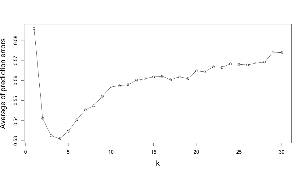
Figure 2 represents the averages of prediction errors for various bandwidth values $k$. The minimum error is attained at $k=4$. None of the above methods achieves the optimal bandwidth $k=4$, but the bandwidth obtained from our method is closest to 4.

5 Discussion

Throughout the paper, we assumed that each row of the Cholesky factor has the same bandwidth for simplicity. It can be extended to more general setting allowing different bandwidth for each row. If we denote the bandwidth for the $j$th row as $k_{0}^{(j)}$ and $k_{0,\max}=\max_{1\leq j\leq p}k_{0}^{(j)}$, then one can conduct the bandwidth test for $k_{0,\max}$. Theoretical results in this paper also hold for the maximum bandwidth $k_{0,\max}$ selection problem with possibly some additional conditions. For example, if $k_{0}^{(j)}=k_{0,\max}$ except only finite $j$’s, then the proposed priors still achieve the theoretical properties in Section 3.

The bandwidth selection problem for bandable matrices is one of the interesting future research topics. Note that it has very different characteristics from that for banded matrices. In the bandable case, the bandwidth selection is to find the optimal bandwidth minimizing the estimation error with respect to some loss function. It is well known that the optimal bandwidth depends on the loss function (Cai et al., 2010). Thus, if the bandwidth selection of the bandable matrix is of primary interest, the prior distribution should be chosen carefully depending on the loss function.

Acknowledgement

We thank Baiguo An for providing us the telephone call center data.

Appendix 1: Posterior convergence rate for the Cholesky factor

The estimation of Cholesky factor is important to detect the dependence structure of data. Although our primary goals are Bayesian bandwidth test and model selection, we show in this section that the proposed prior can be used to estimate Cholesky factors. Theorem 3.1 implies that $\widehat{k}=\operatorname*{argmax}_{0\leq k\leq R_{n}}\pi(k\mid{\bf X}_{n})$ is a consistent estimator of $k_{0}$. Consider an empirical Bayes approach by considering priors (4) and (5) with $\widehat{k}$ instead of imposing a prior on $k$. This empirical Bayes method faciliates easy implementations when the estimation of Cholesky factor or precision matrix is of interest. To assess the performance, we adopt the P-loss convergence rate used by Castillo (2014) and Lee and Lee (2018). Corollary .1 presents the P-loss convergence rate of the empirical Bayes approach with respect to the Cholesky factor under the matrix $\ell_{\infty}$-norm. We denote $\pi_{(k)}$ as the empirical prior stated above and $\mathbb{E}^{\pi_{(k)}}(\cdot\mid{\bf X}_{n})$ as the posterior expectation induced the prior $\pi_{(k)}$.

Corollary .1

Consider model (1) and priors (4) and (5) with $\widehat{k}$ instead of $k$. If conditions (A1)–(A4) are satisfied and $k_{0}+\log p=o(n)$, then we have

$\displaystyle\mathbb{E}_{0}\mathbb{E}^{\pi_{(k)}}\Big{(}\|A_{n}-A_{0n}\|_{\infty}\mid{\bf X}_{n}\Big{)}$ $\displaystyle\lesssim$ $\displaystyle\left(\frac{k_{0}(k_{0}+\log p)}{n}\right)^{\frac{1}{2}}.$

Define a class of precision matrices

$\displaystyle{\cal{U}}_{p}\,\,=\,\,{\cal{U}}_{p}(\epsilon_{0n},\zeta_{0n},M_{\rm bm},\tau,R_{n})$ $\displaystyle=$ $\displaystyle\bigg{\{}\Omega\in\mathcal{C}_{p}:\,\,\Omega\text{ satisfies (A1)}--(A3)\,\,\bigg{\}},$

where $\mathcal{C}_{p}$ is the class of $p\times p$ symmetric positive definite matrices. With a slight modification of Example 13.12 in an unpublished lecture note of John Duchi, the minimax lower bound is given by

$\displaystyle\inf_{k}\inf_{\widehat{A}_{nk}}\sup_{\Omega_{0n}\in{\cal{U}}_{p}}\mathbb{E}_{0}\Big{(}\|\widehat{A}_{nk}-A_{0n}\|_{\infty}\Big{)}$ $\displaystyle\gtrsim$ $\displaystyle\frac{k_{0}}{\sqrt{n}},$

where the second infimum is taken over all estimators with bandwidth $k$. Thus, the above empirical Bayes approach achieves nearly optimal P-loss convergence rate.

Appendix 2: Proofs

  • Proof of Theorem 3.1

    For any $k=0,1,\ldots,R_{n}$, we have

    $\displaystyle\pi(k\mid{\bf X}_{n})$ $\displaystyle\leq$ $\displaystyle\frac{\pi(k\mid{\bf X}_{n})}{\pi(k_{0}\mid{\bf X}_{n})}=\frac{\pi(k)}{\pi(k_{0})}\prod_{j=2}^{p}\left(1+\frac{1}{\gamma}\right)^{-\frac{k_{j}-k_{0j}}{2}}\left(\frac{\widehat{d}_{j}^{(k)}}{\widehat{d}_{j}^{(k_{0})}}\right)^{-\frac{(1-\tau)n}{2}}.$

    Note that

    $\displaystyle\mathbb{E}_{0}\Big{[}\pi(k\neq k_{0}\mid{\bf X}_{n})\Big{]}$ $\displaystyle=$ $\displaystyle\sum_{k>k_{0}}\mathbb{E}_{0}\Big{[}\pi(k\mid{\bf X}_{n})\Big{]}+\sum_{k<k_{0}}\mathbb{E}_{0}\Big{[}\pi(k\mid{\bf X}_{n})\Big{]}.$ (19)

    We will show that the right hand side terms in (19) are of order $o(1)$. Because $\widehat{d}_{j}^{(k)}/\widehat{d}_{j}^{(k_{0})}\sim Beta((n-k_{j})/2,(k_{j}-k_{0j})/2)$ for any $k>k_{0}$, the first term in (19) is bounded above by

    $\displaystyle\frac{\pi(k)}{\pi(k_{0})}\prod_{j=2}^{p}\left(1+\frac{1}{\gamma}\right)^{-\frac{k_{j}-k_{0j}}{2}}\cdot\frac{\Gamma\big{(}\frac{n-k_{0j}}{2}\big{)}\Gamma\big{(}\frac{\tau n-k_{j}}{2}\big{)}}{\Gamma\big{(}\frac{n-k_{j}}{2}\big{)}\Gamma\big{(}\frac{\tau n-k_{0j}}{2}\big{)}}$
    $\displaystyle\leq$ $\displaystyle\frac{\pi(k)}{\pi(k_{0})}\prod_{j=2}^{p}\left(1+\frac{1}{\gamma}\right)^{-\frac{k_{j}-k_{0j}}{2}}\left(\frac{1-(k_{0j}+2)n^{-1}}{\tau-k_{j}n^{-1}}\right)^{\frac{k_{j}-k_{0j}}{2}}$

    provided that $\tau n>R_{n}$. By condition (A3), we have $R_{n}/n\leq\tau\epsilon_{1}/(1+\epsilon_{1})$,

    $\displaystyle\frac{1-(k_{0j}+2)n^{-1}}{\tau-k_{j}n^{-1}}$ $\displaystyle\leq$ $\displaystyle\frac{1+\epsilon_{1}}{\tau},$

    which implies

    $\displaystyle\sum_{k>k_{0}}\mathbb{E}_{0}\Big{[}\pi(k\mid{\bf X}_{n})\Big{]}$ $\displaystyle\leq$ $\displaystyle\sum_{k>k_{0}}\frac{\pi(k)}{\pi(k_{0})}\left\{\Big{(}1+\frac{1}{\gamma}\Big{)}\cdot\Big{(}\frac{\tau}{1+\epsilon_{1}}\Big{)}\right\}^{-\frac{k-k_{0}}{2}\cdot(p-\frac{k+k_{0}+1}{2})}.$

    The last display is of order $o(1)$ by (9).

    It is easy to check that

    $\displaystyle\left(\frac{\widehat{d}_{j}^{(k)}}{\widehat{d}_{j}^{(k_{0})}}\right)^{-\frac{(1-\tau)n}{2}}$ $\displaystyle\leq$ $\displaystyle\exp\left(\frac{1-\tau}{2d_{0j}(1+\widehat{Q}_{jk})}\cdot n(\widehat{d}_{j}^{(k_{0})}-\widehat{d}_{j}^{(k)})\right),$ (20)

    where $\widehat{Q}_{jk}=\widehat{d}_{j}^{(k_{0})}/d_{0j}-1+(\widehat{d}_{j}^{(k)}-\widehat{d}_{j}^{(k_{0})})/d_{0j}$. To deal with $\widehat{d}_{j}^{(k)}$ and $\widehat{Q}_{jk}$ easily, for a given constant $\epsilon=(\tau/10)^{2}$, we define the following sets

    $\displaystyle N_{j}^{c}$ $\displaystyle=$ $\displaystyle\left\{{\bf X}_{n}:\zeta_{0n}^{-1}(1-2\epsilon)^{2}\leq n^{-1}\lambda_{\min}({\bf X}_{j(k_{0})}^{T}{\bf X}_{j(k_{0})})\leq n^{-1}\lambda_{\max}({\bf X}_{j(k_{0})}^{T}{\bf X}_{j(k_{0})})\leq\epsilon_{0n}^{-1}(1+2\epsilon)^{2}\right\},$
    $\displaystyle N_{1,j}^{c}$ $\displaystyle=$ $\displaystyle\left\{{\bf X}_{n}:\bigg{|}\frac{\widehat{d}_{j}^{(k_{0})}}{d_{0j}}-1\bigg{|}\in\Big{(}-4\sqrt{\epsilon}\frac{n-k_{0_{j}}}{n}-\frac{k_{0j}}{n},4\sqrt{\epsilon}\frac{n-k_{0_{j}}}{n}-\frac{k_{0j}}{n}\Big{)}\right\},$
    $\displaystyle N_{2,j,k}^{c}$ $\displaystyle=$ $\displaystyle\left\{{\bf X}_{n}:0<\frac{\widehat{d}_{j}^{(k)}-\widehat{d}_{j}^{(k_{0})}}{d_{0j}}<\epsilon+\frac{\widehat{\lambda}_{jk}}{n}\right\}$

    and $N_{j,k}^{c}=N_{j}^{c}\cap N_{1,j}^{c}\cap N_{2,j,k}^{c}$, where $\widehat{\lambda}_{jk}=\|(I_{n}-\tilde{P}_{jk}){\bf X}_{j(k_{0})}a_{0j}^{(k_{0})}\|_{2}^{2}/d_{0j}$. First, we will show that the above sets have probabilities tending to 1 as $n\to\infty$. Note that $n\widehat{d}_{j}^{(k_{0})}/d_{0j}\sim\chi^{2}_{n-k_{0j}}$ and $n(\widehat{d}_{j}^{(k)}-\widehat{d}_{j}^{(k_{0})})/d_{0j}\sim\chi^{2}_{k_{0j}-k_{j}}(\widehat{\lambda}_{jk})$, where $\chi^{2}_{m}(\lambda)$ denotes the noncentral chi-square distribution with degrees of freedom $m$ and the noncentrality parameter $\lambda$ and $\chi_{m}^{2}=\chi_{m}^{2}(0)$. By Corollary 5.35 in Eldar and Kutyniok (2012), $\mathbb{P}_{0}(N_{j})\leq 4\exp(-n\epsilon^{2}/2)$ for all sufficiently large $n$. From the concentration inequality of chi-square random variable (Lemma 1 in Laurent and Massart (2000)), it is easy to see that $\mathbb{P}_{0}(N_{1,j})\leq 2\exp(-\epsilon(n-k_{0}))$ for all sufficiently large $n$. Finally, by Lemma 4 in Shin et al. (2018), we have

    $\displaystyle\mathbb{P}_{0}(N_{2,j,k})$ $\displaystyle\lesssim$ $\displaystyle\Big{(}\frac{\epsilon n}{2(k_{0j}-k_{j})}\Big{)}^{\frac{k_{0j}-k_{j}}{2}}\exp\Big{(}{\frac{k_{0j}-k_{j}}{2}-\frac{\epsilon n}{2}}\Big{)}+\mathbb{E}_{0}\bigg{(}\,\frac{\widehat{\lambda}_{jk}}{\epsilon n}e^{-\frac{\epsilon^{2}n^{2}}{32\widehat{\lambda}_{jk}}}\wedge 1\,\bigg{)}$
    $\displaystyle\leq$ $\displaystyle\exp\Big{(}{-\frac{\epsilon n}{4}}\Big{)}+\mathbb{E}_{0}\bigg{[}\,\frac{\widehat{\lambda}_{jk}}{\epsilon n}\exp\bigg{(}{-\frac{\epsilon^{2}n^{2}}{32\widehat{\lambda}_{jk}}}\bigg{)}\cdot I(N_{j}^{c})\,\bigg{]}+\mathbb{P}_{0}(N_{j})$
    $\displaystyle\leq$ $\displaystyle\exp\Big{(}{-\frac{\epsilon n}{4}}\Big{)}+\exp\Big{(}{-\frac{\epsilon^{2}\,\zeta_{0n}^{-1}\epsilon_{0n}n}{128(1+2\epsilon)^{2}}}\Big{)}+4\exp\Big{(}{-\frac{\epsilon^{2}n}{2}}\Big{)},$

    which is of order $o(1)$ provided that $\zeta_{0n}/\epsilon_{0n}=o(n)$. The last inequality holds because

    $\displaystyle\widehat{\lambda}_{jk}$ $\displaystyle\leq$ $\displaystyle\lambda_{\max}({\bf X}_{j(k_{0})}^{T}{\bf X}_{j(k_{0})})\cdot d_{0j}^{-1}\|a_{0j}\|_{2}^{2}$
    $\displaystyle\leq$ $\displaystyle 2n(1+2\epsilon)^{2}\epsilon_{0n}^{-1}\cdot\Big{\{}\|d_{0j}^{-1/2}(e_{j}-a_{0j})\|_{2}^{2}+d_{0j}^{-1}\Big{\}}$
    $\displaystyle\leq$ $\displaystyle 2n(1+2\epsilon)^{2}\epsilon_{0n}^{-1}\cdot\zeta_{0n}$

    on $N_{j}^{c}$ for all sufficiently large $n$, where $e_{j}$ is the unit vector whose $j$th element is 1 and the others are zero. Note that

    $\displaystyle\sum_{k<k_{0}}\mathbb{E}_{0}\Big{[}\pi(k\mid{\bf X}_{n})\Big{]}$ $\displaystyle\leq$ $\displaystyle\sum_{k<k_{0}}\sum_{j=2}^{p}\mathbb{P}_{0}(N_{j,k})+\sum_{k<k_{0}}\mathbb{E}_{0}\Big{[}\pi(k\mid{\bf X}_{n})\prod_{j=2}^{p}I(N_{j,k}^{c})\Big{]}.$ (21)

    By the above arguments, (21) is of order $o(1)$ provided that $\zeta_{0n}\log p/\epsilon_{0n}=o(n)$. Thus, the proof is completed if we prove that (21) is of order $o(1)$.

    From the inequality (20),

    $\displaystyle\sum_{k<k_{0}}\mathbb{E}_{0}\Big{[}\pi(k\mid{\bf X}_{n})\prod_{j=2}^{p}I(N_{j,k}^{c})\Big{]}$
    $\displaystyle\leq$ $\displaystyle\sum_{k<k_{0}}\mathbb{E}_{0}\left[\frac{\pi(k)}{\pi(k_{0})}\prod_{j=2}^{p}\Big{(}1+\frac{1}{\gamma}\Big{)}^{\frac{k_{0j}-k_{j}}{2}}\exp\Big{(}\frac{1-\tau}{2d_{0j}(1+\widehat{Q}_{jk})}\cdot n(\widehat{d}_{j}^{(k_{0})}-\widehat{d}_{j}^{(k)})\Big{)}I(N_{j,k}^{c})\right].$

    On the event $N_{j,k}^{c}$, we have

    $\displaystyle\widehat{Q}_{jk}$ $\displaystyle\leq$ $\displaystyle 4\sqrt{\epsilon}\frac{n-k_{0}}{n}-\frac{k_{0}}{n}+\epsilon+\frac{\widehat{\lambda}_{jk}}{n}$
    $\displaystyle\leq$ $\displaystyle 5\sqrt{\epsilon}+\frac{\widehat{\lambda}_{jk}}{n},$
    $\displaystyle\widehat{Q}_{jk}$ $\displaystyle\geq$ $\displaystyle-4\sqrt{\epsilon}\frac{n-k_{0}}{n}-\frac{k_{0}}{n}\,\,\geq\,\,-5\sqrt{\epsilon}$

    for all sufficiently large $n$. For a given $k<k_{0}$,

    $\displaystyle n(\widehat{d}_{j}^{(k_{0})}-\widehat{d}_{j}^{(k)})$ $\displaystyle=$ $\displaystyle\tilde{X}_{j}^{T}(\tilde{P}_{jk}-\tilde{P}_{jk_{0}})\tilde{X}_{j}$
    $\displaystyle\overset{d}{\equiv}$ $\displaystyle-\|(I_{n}-\tilde{P}_{jk}){\bf X}_{j(k_{0})}a_{0j}^{(k_{0})}\|_{2}^{2}-2\tilde{\epsilon}_{j}^{T}(I_{n}-\tilde{P}_{jk}){\bf X}_{j(k_{0})}a_{0j}^{(k_{0})}+\tilde{\epsilon}_{j}^{T}(\tilde{P}_{jk}-\tilde{P}_{jk_{0}})\tilde{\epsilon}_{j}$
    $\displaystyle\leq$ $\displaystyle-d_{0j}\widehat{\lambda}_{jk}-2\tilde{\epsilon}_{j}^{T}(I_{n}-\tilde{P}_{jk}){\bf X}_{j(k_{0})}a_{0j}^{(k_{0})}$
    $\displaystyle=:$ $\displaystyle-d_{0j}\widehat{\lambda}_{jk}-2V_{jk},$

    where $\tilde{\epsilon}_{j}\sim N_{n}(0,d_{0j}I_{n})$ and $V_{jk}/\sqrt{d_{0j}}\sim N(0,d_{0j}\widehat{\lambda}_{jk})$ under $\mathbb{P}_{0}$ given ${\bf X}_{j(k_{0})}$. Then,

    $\displaystyle\mathbb{E}_{0}\left[\exp\Big{(}\frac{1-\tau}{2d_{0j}(1+\widehat{Q}_{jk})}\cdot n(\widehat{d}_{j}^{(k_{0})}-\widehat{d}_{j}^{(k)})\Big{)}\mid{\bf X}_{j(k_{0})}\right]I(N_{j,k}^{c})$
    $\displaystyle\leq$ $\displaystyle\mathbb{E}_{0}\left[\exp\Big{(}-\frac{1-\tau}{2d_{0j}(1+\widehat{Q}_{jk})}\cdot(d_{0j}\widehat{\lambda}_{jk}+2V_{jk})\Big{)}\mid{\bf X}_{j(k_{0})}\right]I(N_{j,k}^{c}).$

    From the moment generating function of the normal distribution, we have

    $\displaystyle\mathbb{E}_{0}\left[\exp\Big{(}-\frac{1-\tau}{2d_{0j}(1+Q)}\cdot(d_{0j}\widehat{\lambda}_{jk}+2V_{jk})\Big{)}\mid{\bf X}_{j(k_{0})}\right]I(N_{j,k}^{c})$
    $\displaystyle\leq$ $\displaystyle\exp\Big{\{}-\frac{1-\tau}{2(1+Q)}\Big{(}1-\frac{1-\tau}{1+Q}\Big{)}\,\widehat{\lambda}_{jk}\Big{\}}I(N_{j,k}^{c})$
    $\displaystyle\leq$ $\displaystyle\exp\Big{\{}-\frac{1-\tau}{2(1+5\sqrt{\epsilon}+\widehat{\lambda}_{jk}/n)}\Big{(}1-\frac{1-\tau}{1-5\sqrt{\epsilon}}\Big{)}\,\widehat{\lambda}_{jk}\Big{\}}I(N_{j,k}^{c})$

    for any $Q=-5\sqrt{\epsilon}$ or $Q=5\sqrt{\epsilon}+\widehat{\lambda}_{jk}/n$. Note that

    $\displaystyle d_{0j}\widehat{\lambda}_{jk}$ $\displaystyle=$ $\displaystyle\|(I_{n}-\tilde{P}_{jk}){\bf X}_{j(k_{0})}a_{0j}^{(k_{0})}\|_{2}^{2}$
    $\displaystyle\geq$ $\displaystyle\lambda_{\min}({\bf X}_{j(k_{0})}^{T}{\bf X}_{j(k_{0})})(k_{0j}-k_{j})\min_{j,l:a_{0,jl}\neq 0}|a_{0,jl}|^{2}$
    $\displaystyle\geq$ $\displaystyle n\zeta_{0n}^{-1}(1-2\epsilon)^{2}(k_{0j}-k_{j})\min_{j,l:a_{0,jl}\neq 0}|a_{0,jl}|^{2}$

    on ${\bf X}_{n}\in N_{j,k}^{c}$ by Lemma 5 in Arias-Castro and Lounici (2014) and $1-(1-\tau)/(1-5\sqrt{\epsilon})>\tau/2$ by the definition of $\epsilon$. Thus,

    $\displaystyle\frac{1-\tau}{2(1+5\sqrt{\epsilon}+\widehat{\lambda}_{jk}/n)}\Big{(}1-\frac{1-\tau}{1-5\sqrt{\epsilon}}\Big{)}\,\widehat{\lambda}_{jk}$
    $\displaystyle\geq$ $\displaystyle\frac{\tau(1-\tau)}{4}\cdot\Big{(}\frac{1+5\sqrt{\epsilon}}{\widehat{\lambda}_{jk}}+\frac{1}{n}\Big{)}^{-1}$
    $\displaystyle\geq$ $\displaystyle\frac{\tau(1-\tau)}{4}\cdot\Big{(}\frac{(1+5\sqrt{\epsilon})\epsilon_{0n}^{-1}\zeta_{0n}}{(1-2\epsilon)^{2}(k_{0j}-k_{j})\min_{j,l:a_{0,jl}\neq 0}|a_{0,jl}|^{2}n}+\frac{1}{n}\Big{)}^{-1}$
    $\displaystyle\geq$ $\displaystyle\frac{\tau(1-\tau)}{4}\cdot\Big{(}\frac{(1+5\sqrt{\epsilon})}{(1-2\epsilon)^{2}(k_{0j}-k_{j})C_{\rm bm}}+\frac{1}{n}\Big{)}^{-1}$
    $\displaystyle\geq$ $\displaystyle\frac{\tau(1-\tau)}{8}\cdot\frac{(1-2\epsilon)^{2}(k_{0j}-k_{j})C_{\rm bm}}{(1+5\sqrt{\epsilon})}$
    $\displaystyle\geq$ $\displaystyle(k_{0j}-k_{j})M_{\rm bm}$

    on ${\bf X}_{n}\in N_{j,k}^{c}$ by condition (A2), the definition of $\epsilon$ and $\tau\leq 0.4$, where $C_{\rm bm}=10\tau^{-1}(1-\tau)^{-1}M_{\rm bm}$. It implies that (21) is bounded above by

    $\displaystyle\sum_{k<k_{0}}\frac{\pi(k)}{\pi(k_{0})}\prod_{j=2}^{p}\Big{(}1+\frac{1}{\gamma}\Big{)}^{\frac{k_{0j}-k_{j}}{2}}\cdot 2(e^{-M_{\rm bm}})^{k_{0j}-k_{j}}$
    $\displaystyle\leq$ $\displaystyle\sum_{k<k_{0}}\frac{\pi(k)}{\pi(k_{0})}\prod_{j=2}^{p}\left\{2\Big{(}1+\frac{1}{\gamma}\Big{)}^{\frac{1}{2}}e^{-M_{\rm bm}}\right\}^{k_{0j}-k_{j}}$
    $\displaystyle=$ $\displaystyle\sum_{k<k_{0}}\frac{\pi(k)}{\pi(k_{0})}\left\{2\Big{(}1+\frac{1}{\gamma}\Big{)}^{\frac{1}{2}}e^{-M_{\rm bm}}\right\}^{(k_{0}-k)\big{(}p-\frac{k+k_{0}+1}{2}\big{)}},$

    which is of order $o(1)$ provided that (10).

  • Proof of Theorem 3.2

    Note that

    $\displaystyle B_{10}({\bf X}_{n})$ $\displaystyle=$ $\displaystyle\frac{p({\bf X}_{n}\mid H_{1})}{p({\bf X}_{n}\mid H_{0})}$
    $\displaystyle=$ $\displaystyle\frac{\sum_{k>k^{\star}}\int p({\bf X}_{n}\mid\Omega_{n},k)\pi(\Omega_{n}\mid k)\pi_{1}(k)d\Omega_{n}}{\sum_{k\leq k^{\star}}\int p({\bf X}_{n}\mid\Omega_{n},k)\pi(\Omega_{n}\mid k)\pi_{0}(k)d\Omega_{n}}$
    $\displaystyle=$ $\displaystyle\frac{\sum_{k>k^{\star}}p({\bf X}_{n}\mid k)\pi_{1}(k)}{\sum_{k\leq k^{\star}}\int p({\bf X}_{n}\mid k)\pi_{0}(k)}$
    $\displaystyle=$ $\displaystyle\frac{\pi(k>k^{\star}\mid{\bf X}_{n})}{\pi(k\leq k^{\star}\mid{\bf X}_{n})}\times\frac{C_{0}}{C_{1}}$

    and $C_{0}/C_{1}=k^{\star}/(R_{n}-k^{\star})$.

    If $H_{0}:k\leq k^{\star}$ is true, i.e. $k_{0}\leq k^{\star}$,

    $\displaystyle\mathbb{E}_{0}\Big{[}B_{10}({\bf X}_{n})\Big{]}$ $\displaystyle\leq$ $\displaystyle\mathbb{E}_{0}\Big{[}\frac{\pi(k>k^{\star}\mid{\bf X}_{n})}{\pi(k=k_{0}\mid{\bf X}_{n})}\Big{]}\times\frac{k^{\star}}{R_{n}-k^{\star}}$
    $\displaystyle\leq$ $\displaystyle\sum_{k>k^{\star}}\mathbb{E}_{0}\Big{[}\frac{\pi(k\mid{\bf X}_{n})}{\pi(k_{0}\mid{\bf X}_{n})}\Big{]}\times\frac{k^{\star}}{R_{n}-k^{\star}}$
    $\displaystyle\leq$ $\displaystyle k^{\star}\cdot\left\{\frac{(1+\gamma)\tau}{\gamma(1+\tau)}\right\}^{-\frac{k^{\star}+1-k_{0}}{2}\cdot(p-\frac{R_{n}+k_{0}+1}{2})}=T_{n,H_{0},k_{0},k^{\star}},$

    which implies

    $\displaystyle B_{10}({\bf X}_{n})$ $\displaystyle=$ $\displaystyle O_{p}\big{(}T_{n,H_{0},k_{0},k^{\star}}\big{)}\quad\text{ under }H_{0}.$

    On the other hand, if $H_{1}:k>k^{\star}$ is true, i.e. $k_{0}>k^{\star}$,

    $\displaystyle\mathbb{E}_{0}\Big{[}\frac{\sum_{k\leq k^{\star}}\pi(k\mid{\bf X}_{n})\prod_{j=2}^{p}I(N_{j,k}^{c})}{\pi(k_{0}\mid{\bf X}_{n})}\Big{]}\times\frac{R_{n}-k^{\star}}{k^{\star}}$
    $\displaystyle\leq$ $\displaystyle\left\{\frac{4(1+\gamma)}{\gamma\exp(2M_{\rm bm})}\right\}^{\frac{k_{0}-k^{\star}}{2}\cdot(p-\frac{k^{\star}+k_{0}+1}{2})}\times(R_{n}-k^{\star})$
    $\displaystyle=$ $\displaystyle T_{n,H_{1},k_{0},k^{\star}}.$

    Now, we will show that for every $\epsilon>0$, there exist a constant $C>0$ and an integer $N$ such that

    $\displaystyle\mathbb{P}_{0}\Big{(}B_{10}({\bf X}_{n})<C^{-1}T_{n,H_{1},k_{0},k^{\star}}^{-1}\Big{)}$ $\displaystyle\leq$ $\displaystyle\epsilon$

    for all $n\geq N$ under $H_{1}$, which implies $B_{10}^{-1}({\bf X}_{n})=O_{p}(T_{n,H_{1},k_{0},k^{\star}})$ under $H_{1}$. Note that

    $\displaystyle\mathbb{P}_{0}\Big{(}B_{10}({\bf X}_{n})\leq C^{-1}T_{n,H_{1},k_{0},k^{\star}}^{-1}\Big{)}$
    $\displaystyle=$ $\displaystyle\mathbb{P}_{0}\Big{(}B_{10}({\bf X}_{n})^{-1}\geq CT_{n,H_{1},k_{0},k^{\star}}\Big{)}$
    $\displaystyle\leq$ $\displaystyle\mathbb{P}_{0}\Big{(}\frac{\sum_{k\leq k^{\star}}\pi(k\mid{\bf X}_{n})}{\pi(k_{0}\mid{\bf X}_{n})}\geq\frac{k^{\star}CT_{n,H_{1},k_{0},k^{\star}}}{R_{n}-k^{\star}}\Big{)}.$

    Let $N_{j,k}$ be the set defined in the proof of Theorem 3.1, then the last term is bounded above by

    $\displaystyle\mathbb{P}_{0}\Big{(}\frac{\sum_{k\leq k^{\star}}\pi(k\mid{\bf X}_{n})\prod_{j=2}^{p}I(N_{j,k}^{c})}{\pi(k_{0}\mid{\bf X}_{n})}\geq\frac{k^{\star}CT_{n,H_{1},k_{0},k^{\star}}}{R_{n}-k^{\star}}\Big{)}+\sum_{k\leq k^{\star}}\sum_{j=2}^{p}\mathbb{P}_{0}(N_{j,k})$
    $\displaystyle\leq$ $\displaystyle\mathbb{E}_{0}\Big{[}\frac{\sum_{k\leq k^{\star}}\pi(k\mid{\bf X}_{n})\prod_{j=2}^{p}I(N_{j,k}^{c})}{\pi(k_{0}\mid{\bf X}_{n})}\Big{]}\times\frac{R_{n}-k^{\star}}{k^{\star}CT_{n,H_{1},k_{0},k^{\star}}}+o(1)$
    $\displaystyle\leq$ $\displaystyle\frac{1}{C}+o(1).$

    Thus, it completes the proof.

  • Proof of Theorem 3.3

    It is easy to see that

    $\displaystyle B_{10}({\bf X}_{n_{1}},{\bf Y}_{n_{2}})$ $\displaystyle=$ $\displaystyle\frac{p({\bf X}_{n_{1}},{\bf Y}_{n_{2}}\mid H_{1})}{p({\bf X}_{n_{1}},{\bf Y}_{n_{2}}\mid H_{0})}$
    $\displaystyle=$ $\displaystyle\frac{\sum_{k_{1}\neq k_{2}}\pi(k_{1}\mid{\bf X}_{n_{1}})\pi(k_{2}\mid{\bf Y}_{n_{2}})}{\sum_{k_{1}=k_{2}}\pi(k_{1}\mid{\bf X}_{n_{1}})\pi(k_{2}\mid{\bf Y}_{n_{2}})}\times R_{n}^{-1}.$

    If $H_{0}:k_{1}=k_{2}$ is true, let $k_{01}=k_{02}=k_{0}$, then

    $\displaystyle B_{10}({\bf X}_{n_{1}},{\bf Y}_{n_{2}})$ $\displaystyle\leq$ $\displaystyle\frac{\sum_{k_{1}\neq k_{2}}\pi(k_{1}\mid{\bf X}_{n_{1}})\pi(k_{2}\mid{\bf Y}_{n_{2}})}{\pi(k_{0}\mid{\bf X}_{n_{1}})\pi(k_{0}\mid{\bf Y}_{n_{2}})}\times R_{n}^{-1}$
    $\displaystyle\leq$ $\displaystyle\sum_{k_{1}=1}^{R_{n}}\frac{\pi(k_{1}\mid{\bf X}_{n_{1}})}{\pi(k_{0}\mid{\bf X}_{n_{1}})}\max_{k_{2}\neq k_{1}}\frac{\pi(k_{2}\mid{\bf Y}_{n_{2}})}{\pi(k_{0}\mid{\bf Y}_{n_{2}})}.$

    Note that

    $\displaystyle\frac{\pi(k_{0}\mid{\bf X}_{n_{1}})}{\pi(k_{0}\mid{\bf X}_{n_{1}})}\max_{k_{2}\neq k_{0}}\frac{\pi(k_{2}\mid{\bf Y}_{n_{2}})}{\pi(k_{0}\mid{\bf Y}_{n_{2}})}$ $\displaystyle=$ $\displaystyle\max_{k_{2}\neq k_{0}}\frac{\pi(k_{2}\mid{\bf Y}_{n_{2}})}{\pi(k_{0}\mid{\bf Y}_{n_{2}})}$
    $\displaystyle=$ $\displaystyle O_{p}\left(\frac{1}{R_{n}-k_{0}}T_{n,H_{1},k_{0},k_{0}-1}+\frac{1}{k_{0}}T_{n,H_{0},k_{0},k_{0}}\right)$

    and

    $\displaystyle\sum_{k_{1}\neq k_{0}}\frac{\pi(k_{1}\mid{\bf X}_{n_{1}})}{\pi(k_{0}\mid{\bf X}_{n_{1}})}\max_{k_{2}\neq k_{1}}\frac{\pi(k_{2}\mid{\bf Y}_{n_{2}})}{\pi(k_{0}\mid{\bf Y}_{n_{2}})}$
    $\displaystyle=$ $\displaystyle O_{p}\left(\frac{k_{0}}{R_{n}-k_{0}}T_{n,H_{1},k_{0},k_{0}-1}+\frac{R_{n}-k_{0}}{k_{0}}T_{n,H_{0},k_{0},k_{0}}\right).$

    Thus, we have under $H_{0}$,

    $\displaystyle B_{10}({\bf X}_{n_{1}},{\bf Y}_{n_{2}})$ $\displaystyle=$ $\displaystyle O_{p}\left(\frac{k_{0}}{R_{n}-k_{0}}T_{n,H_{1},k_{0},k_{0}-1}+\frac{R_{n}-k_{0}}{k_{0}}T_{n,H_{0},k_{0},k_{0}}\right).$

    On the other hand, if $H_{1}:k_{1}\neq k_{2}$ is true,

    $\displaystyle B_{10}({\bf X}_{n_{1}},{\bf Y}_{n_{2}})^{-1}$ $\displaystyle\leq$ $\displaystyle\frac{\sum_{k_{1}=k_{2}}\pi(k_{1}\mid{\bf X}_{n_{1}})\pi(k_{2}\mid{\bf Y}_{n_{2}})}{\pi(k_{01}\mid{\bf X}_{n_{1}})\pi(k_{02}\mid{\bf Y}_{n_{2}})}\times R_{n}.$

    Note that

    $\displaystyle\frac{\pi(k_{01}\mid{\bf X}_{n_{1}})\pi(k_{01}\mid{\bf Y}_{n_{2}})}{\pi(k_{01}\mid{\bf X}_{n_{1}})\pi(k_{02}\mid{\bf Y}_{n_{2}})}\times R_{n}$ $\displaystyle=$ $\displaystyle\frac{\pi(k_{01}\mid{\bf Y}_{n_{2}})}{\pi(k_{02}\mid{\bf Y}_{n_{2}})}\times R_{n}$
    $\displaystyle=$ $\displaystyle O_{p}\left(\frac{R_{n}}{R_{n}-k_{01}}T_{n,H_{1},k_{02},k_{01}}+\frac{R_{n}}{k_{01}}T_{n,H_{0},k_{02},k_{01}}\right)$

    and

    $\displaystyle\frac{\sum_{k_{1}=k_{2}\neq k_{01}}\pi(k_{1}\mid{\bf X}_{n_{1}})\pi(k_{2}\mid{\bf Y}_{n_{2}})}{\pi(k_{01}\mid{\bf X}_{n_{1}})\pi(k_{02}\mid{\bf Y}_{n_{2}})}\times R_{n}$
    $\displaystyle\leq$ $\displaystyle\sum_{k_{1}\neq k_{01}}\frac{\pi(k_{1}\mid{\bf X}_{n_{1}})}{\pi(k_{01}\mid{\bf X}_{n_{1}})}\max_{k_{2}}\frac{\pi(k_{2}\mid{\bf Y}_{n_{1}})}{\pi(k_{02}\mid{\bf Y}_{n_{1}})}\times R_{n}$
    $\displaystyle=$ $\displaystyle O_{p}\left(\frac{R_{n}\,k_{01}}{R_{n}-k_{01}}T_{n,H_{1},k_{01},k_{01}-1}+\frac{R_{n}(R_{n}-k_{01})}{k_{01}}T_{n,H_{0},k_{01},k_{01}}\right).$

    Thus, we have

    $\displaystyle B_{10}({\bf X}_{n_{1}},{\bf Y}_{n_{2}})^{-1}$ $\displaystyle=$ $\displaystyle O_{p}\left(\frac{R_{n}\,k_{01}}{R_{n}-k_{01}}T_{n,H_{1},k_{01},k_{01}-1}+\frac{R_{n}(R_{n}-k_{01})}{k_{01}}T_{n,H_{0},k_{01},k_{01}}\right).$

    Similarly, it is easy to show that

    $\displaystyle B_{10}({\bf X}_{n_{1}},{\bf Y}_{n_{2}})^{-1}$ $\displaystyle=$ $\displaystyle O_{p}\left(\frac{R_{n}\,k_{02}}{R_{n}-k_{02}}T_{n,H_{1},k_{02},k_{02}-1}+\frac{R_{n}(R_{n}-k_{02})}{k_{02}}T_{n,H_{0},k_{02},k_{02}}\right).$

    Let $k_{\min}=k_{01}\wedge k_{02}$, then under $H_{1}$ one has

    $\displaystyle B_{10}({\bf X}_{n_{1}},{\bf Y}_{n_{2}})^{-1}$ $\displaystyle=$ $\displaystyle O_{p}\left(\frac{R_{n}\,k_{\min}}{R_{n}-k_{\min}}T_{n,H_{1},k_{\min},k_{\min}-1}+\frac{R_{n}(R_{n}-k_{\min})}{k_{\min}}T_{n,H_{0},k_{\min},k_{\min}}\right).$
  • Proof of Corollary .1

    By the proof of Theorem 3.1, we have

    $\displaystyle\mathbb{E}_{0}\big{[}\pi(k\neq k_{0}\mid{\bf X}_{n})\big{]}$ $\displaystyle\lesssim$ $\displaystyle C_{\star}^{-(p-k_{0}-1)},$

    where $C_{\star}>0$ is a constant depending on $\gamma,\tau$ and $M_{\rm bm}$. By the Markov’s inequality,

    $\displaystyle\mathbb{P}_{0}(\widehat{k}\neq k_{0})$ $\displaystyle\leq$ $\displaystyle\mathbb{P}_{0}(\pi(k\neq k_{0}\mid{\bf X}_{n})>1/2)$ (22)
    $\displaystyle\leq$ $\displaystyle 2\,\mathbb{E}_{0}\big{[}\pi(k\neq k_{0}\mid{\bf X}_{n})\big{]},$

    where $\widehat{k}=\operatorname*{argmax}_{k}\pi(k\mid{\bf X}_{n})$.

    Note that

    $\displaystyle\mathbb{E}_{0}\mathbb{E}^{\pi_{(k)}}\Big{(}\|A_{n}-A_{0n}\|_{\infty}\mid{\bf X}_{n}\Big{)}$ (23)
    $\displaystyle=$ $\displaystyle\mathbb{E}_{0}\Big{[}\mathbb{E}^{\pi_{(k)}}\Big{(}\|A_{n}-A_{0n}\|_{\infty}\mid{\bf X}_{n}\Big{)}I(\widehat{k}=k_{0})\Big{]}+\mathbb{E}_{0}\Big{[}\mathbb{E}^{\pi_{(k)}}\Big{(}\|A_{n}-A_{0n}\|_{\infty}\mid{\bf X}_{n}\Big{)}I(\widehat{k}\neq k_{0})\Big{]}.\quad\quad$

    The first term in (23) is of order $(k_{0}(k_{0}+\log p)/n)^{1/2}$ by Lemmas 2 and 4 in Lee and Lee (2017). The second term in (23) is bounded above by

    $\displaystyle\Big{\{}\mathbb{E}_{0}\mathbb{E}^{\pi_{(k)}}\big{(}\|A_{n}-A_{0n}\|_{\infty}^{2}\mid{\bf X}_{n}\big{)}\Big{\}}^{\frac{1}{2}}\,\left\{\mathbb{P}_{0}(\widehat{k}\neq k_{0})\right\}^{\frac{1}{2}}\lesssim\left(\frac{k_{0}(k_{0}+\log p)}{n}\right)^{\frac{1}{2}}$

    by (22) and Lemmas 2 and 4 in Lee and Lee (2017).

References

  • (1)
  • An et al. (2014) An, B., Guo, J. and Liu, Y. (2014). Hypothesis testing for band size detection of high-dimensional banded precision matrices, Biometrika 101(2): 477–483.
  • Arias-Castro and Lounici (2014) Arias-Castro, E. and Lounici, K. (2014). Estimation and variable selection with exponential weights, Electronic Journal of Statistics 8(1): 328–354.
  • Banerjee and Ghosal (2014) Banerjee, S. and Ghosal, S. (2014). Posterior convergence rates for estimating large precision matrices using graphical models, Electronic Journal of Statistics 8(2): 2111–2137.
  • Banerjee and Ghosal (2015) Banerjee, S. and Ghosal, S. (2015). Bayesian structure learning in graphical models, Journal of Multivariate Analysis 136: 147–162.
  • Bickel and Levina (2008) Bickel, P. J. and Levina, E. (2008). Regularized estimation of large covariance matrices, The Annals of Statistics 36(1): 199–227.
  • Cai et al. (2013) Cai, T. T., Liu, W. and Xia, Y. (2013). Two-sample covariance matrix testing and support recovery in high-dimensional and sparse settings, Journal of the American Statistical Association 108(501): 265–277.
  • Cai et al. (2015) Cai, T. T., Ma, Z. and Wu, Y. (2015). Optimal estimation and rank detection for sparse spiked covariance matrices, Probability theory and related fields 161(3-4): 781–815.
  • Cai et al. (2010) Cai, T. T., Zhang, C.-H. and Zhou, H. H. (2010). Optimal rates of convergence for covariance matrix estimation, The Annals of Statistics 38(4): 2118–2144.
  • Cai and Zhou (2012a) Cai, T. T. and Zhou, H. H. (2012a). Minimax estimation of large covariance matrices under $\ell_{1}$-norm, Statistica Sinica pp. 1319–1349.
  • Cao et al. (2017) Cao, X., Khare, K. and Ghosh, M. (2017). Posterior graph selection and estimation consistency for high-dimensional bayesian dag models, arXiv:1611.01205v2 .
  • Castillo (2014) Castillo, I. (2014). On bayesian supremum norm contraction rates, The Annals of Statistics 42(5): 2058–2091.
  • Castillo et al. (2015) Castillo, I., Schmidt-Hieber, J., Van der Vaart, A. et al. (2015). Bayesian linear regression with sparse priors, The Annals of Statistics 43(5): 1986–2018.
  • Cheng et al. (2017) Cheng, G., Zhang, Z. and Zhang, B. (2017). Test for bandedness of high-dimensional precision matrices, Journal of Nonparametric Statistics 29(4): 884–902.
  • Dass and Lee (2004) Dass, S. C. and Lee, J. (2004). A note on the consistency of bayes factors for testing point null versus non-parametric alternatives, Journal of statistical planning and inference 119(1): 143–152.
  • Eldar and Kutyniok (2012) Eldar, Y. C. and Kutyniok, G. (2012). Compressed sensing: theory and applications, Cambridge University Press.
  • Fan et al. (2008) Fan, J., Fan, Y. and Lv, J. (2008). High dimensional covariance matrix estimation using a factor model, Journal of Econometrics 147(1): 186–197.
  • Gao and Zhou (2015) Gao, C. and Zhou, H. H. (2015). Rate-optimal posterior contraction for sparse pca, The Annals of Statistics 43(2): 785–818.
  • Hu and Negahban (2017) Hu, A. and Negahban, S. (2017). Minimax estimation of bandable precision matrices, Advances in Neural Information Processing Systems, pp. 4895–4903.
  • Huang et al. (2006) Huang, J. Z., Liu, N., Pourahmadi, M. and Liu, L. (2006). Covariance matrix selection and estimation via penalised normal likelihood, Biometrika 93(1): 85–98.
  • Johnson and Rossell (2010) Johnson, V. E. and Rossell, D. (2010). On the use of non-local prior densities in bayesian hypothesis tests, Journal of the Royal Statistical Society: Series B (Statistical Methodology) 72(2): 143–170.
  • Johnson and Rossell (2012) Johnson, V. E. and Rossell, D. (2012). Bayesian model selection in high-dimensional settings, Journal of the American Statistical Association 107(498): 649–660.
  • Johnstone and Lu (2009) Johnstone, I. M. and Lu, A. Y. (2009). On consistency and sparsity for principal components analysis in high dimensions, J. Amer. Statist. Assoc. 104(486): 682–693.
  • Laurent and Massart (2000) Laurent, B. and Massart, P. (2000). Adaptive estimation of a quadratic functional by model selection, Annals of Statistics 28(5): 1302–1338.
  • Lee and Lee (2017) Lee, K. and Lee, J. (2017). Estimating large precision matrices via modified cholesky decomposition, arXiv:1707.01143 .
  • Lee and Lee (2018) Lee, K. and Lee, J. (2018). Optimal bayesian minimax rates for unconstrained large covariance matrices, Bayesian Analysis 13(4): 1211–1229.
  • Liang et al. (2008) Liang, F., Paulo, R., Molina, G., Clyde, M. A. and Berger, J. O. (2008). Mixtures of g priors for bayesian variable selection, Journal of the American Statistical Association 103(481): 410–423.
  • Martin et al. (2017) Martin, R., Mess, R. and Walker, S. G. (2017). Empirical bayes posterior concentration in sparse high-dimensional linear models, Bernoulli 23(3): 1822–1847.
  • Moreno et al. (2010) Moreno, E., Girón, F. J. and Casella, G. (2010). Consistency of objective bayes factors as the model dimension grows, The Annals of Statistics pp. 1937–1952.
  • Pati et al. (2014) Pati, D., Bhattacharya, A., Pillai, N. S. and Dunson, D. (2014). Posterior contraction in sparse bayesian factor models for massive covariance matrices, The Annals of Statistics 42(3): 1102–1130.
  • Ren et al. (2015) Ren, Z., Sun, T., Zhang, C.-H., Zhou, H. H. et al. (2015). Asymptotic normality and optimalities in estimation of large gaussian graphical models, The Annals of Statistics 43(3): 991–1026.
  • Rossell and Rubio (2017) Rossell, D. and Rubio, F. J. (2017). Tractable bayesian variable selection: beyond normality, Journal of the American Statistical Association (just-accepted).
  • Roverato (2000) Roverato, A. (2000). Cholesky decomposition of a hyper inverse wishart matrix, Biometrika 87(1): 99–112.
  • Shang and Clayton (2011) Shang, Z. and Clayton, M. K. (2011). Consistency of bayesian linear model selection with a growing number of parameters, Journal of Statistical Planning and Inference 141(11): 3463–3474.
  • Shin et al. (2018) Shin, M., Bhattacharya, A. and Johnson, V. E. (2018). Scalable bayesian variable selection using nonlocal prior densities in ultrahigh-dimensional settings, Statistica Sinica 28(2): 1053.
  • Wang et al. (2016) Wang, M., Maruyama, Y. et al. (2016). Consistency of bayes factor for nonnested model selection when the model dimension grows, Bernoulli 22(4): 2080–2100.
  • Wang and Sun (2014) Wang, M. and Sun, X. (2014). Bayes factor consistency for nested linear models with a growing number of parameters, Journal of Statistical Planning and Inference 147: 95–105.
  • Xiang et al. (2015) Xiang, R., Khare, K. and Ghosh, M. (2015). High dimensional posterior convergence rates for decomposable graphical models, Electronic Journal of Statistics 9(2): 2828–2854.
  • Yang et al. (2016) Yang, Y., Wainwright, M. J. and Jordan, M. I. (2016). On the computational complexity of high-dimensional bayesian variable selection, The Annals of Statistics 44(6): 2497–2532.
  • Zellner (1986) Zellner, A. (1986). On assessing prior distributions and bayesian regression analysis with g-prior distributions, Bayesian inference and decision techniques: Essays in Honor of Bruno De Finetti 6: 233–243.