Quantum generative adversarial networks
Abstract
Quantum machine learning is expected to be one of the first potential general-purpose applications of near-term quantum devices. A major recent breakthrough in classical machine learning is the notion of generative adversarial training, where the gradients of a discriminator model are used to train a separate generative model. In this work and a companion paper, we extend adversarial training to the quantum domain and show how to construct generative adversarial networks using quantum circuits. Furthermore, we also show how to compute gradients – a key element in generative adversarial network training – using another quantum circuit. We give an example of a simple practical circuit ansatz to parametrize quantum machine learning models and perform a simple numerical experiment to demonstrate that quantum generative adversarial networks can be trained successfully.
I Introduction
Deep learning (LeCun et al., 2015; Goodfellow et al., 2016) is currently transforming the way we process large-scale complex data with computers. Deep neural networks are now able to perform image and speech recognition with accuracies at a similar level to humans (Deng, 2014). One of the most exciting recent developments in deep learning is generative adversarial networks (GANs) (Goodfellow et al., 2014). These are a class of deep neural networks which have shown great promise for the task of generative machine learning, that is, learning to generate realistic data samples. Despite the initial difficulties of training these models (Salimans et al., 2016), GANs have quickly found applications in many fields (Creswell et al., 2018), including image generation (Zhu et al., 2016), super-resolution (Ledig et al., 2016), image-to-image translation (Isola et al., 2016), generation of 3D objects (Choy et al., 2016), text generation (Gulrajani et al., 2017), and the generation of synthetic data for chemistry (Kadurin et al., 2017), biology (Killoran et al., 2017), and physics (de Oliveira et al., 2017).
The goal of GANs is to simultaneously train two functions: a generator , and a discriminator , through an adversarial learning strategy. The goal for the generator is to generate new sample data from some specific domain, such as images, text, or audio. The outputs from the generator should not be completely unstructured; rather, they should be plausible samples that reflect the properties of real-world data (e.g., realistic images or natural language). The goal of the discriminator is to distinguish fake data samples which were created by the generator from those which are real.
The training strategy for GANs is anchored in game theory and is analogous to the competition between counterfeiters who have to produce fake currencies and the police who have to design methods to distinguish increasingly more convincing counterfeits from the real ones. This game has a Nash equilibrium where the fake coins become indistinguishable from the real ones and the authorities can no longer devise a method to discriminate the real currencies from the generated ones (Goodfellow et al., 2014) . Interestingly, theoretical proofs regarding the optimal points of adversarial training assume that the generator and discriminator have infinite capacity (Goodfellow et al., 2014), i.e., they can encode arbitrary functions or probability distributions. Yet it is widely believed that classical computers cannot efficiently solve certain hard problems, so these optimal points may be intrinsically out of reach of classical models in many cases of interest.
Quantum computers (Feynman, 1982; Nielsen and Chuang, 2009) have the potential to solve problems believed to be beyond the reach of classical computers, such as factoring large integers (Shor, 1997). Realistic near-term quantum devices (Preskill, 2018) may be able to speed up difficult optimization and sampling problems, even if the full power of fault-tolerant devices may not be available for several years. For instance, variational quantum algorithms (Peruzzo et al., 2014; Kandala et al., 2017; Moll et al., 2017; Giacomo Guerreschi and Smelyanskiy, 2017; Dallaire-Demers et al., 2018), such as the variational quantum eigensolver (VQE), have been demonstrated with great success in the field of quantum chemistry. Currently, these ideas and algorithms are being extended to the domain of quantum machine learning (Schuld et al., 2014; Arjovsky et al., 2015; Romero et al., 2017, 2017; Biamonte et al., 2017; Cao et al., 2017; Verdon et al., 2017; Otterbach et al., 2017; Schuld and Killoran, 2018; Schuld et al., 2018; Huggins et al., 2018; Farhi and Neven, 2018; Mitarai et al., 2018), which could also benefit from a quantum advantage. Since many machine learning algorithms are naturally robust to noise, this direction is a promising application for near-term imperfect quantum devices.
In this paper, we introduce QuGANs, the quantum version of generative adversarial networks. The paper has the following structure. In Section II.1, we generalize the model structure of classical generative adversarial networks (Goodfellow et al., 2014) to define the quantum mechanical equivalent – QuGANs – and provide the cost function for training. A key ingredient for GANs is that the discriminator provides a gradient which the generator can use for gradient-based learning. In Section II.2, we present a general formalism for computing exact gradients of quantum optimization and machine learning problems using quantum circuits. We then show how these gradients can be combined with a classical optimization routine to train QGANs in Section II.3. Finally, we provide an example quantum circuit for both the generator and discriminator in Section II.4 and show that QuGANs can be trained in practice with a simple proof-of-principle numerical experiment in Section II.5.
We will explore the practical issues of QuGANs by explicitly constructing quantum circuits for the generator and discriminator and proposing quantum methods for computing the gradients of these circuits. A more in-depth theoretical exploration of quantum adversarial learning can be found in the companion paper Lloyd and Weedbrook (2018).
II Training QuGANs
II.1 The structure of GANs and QuGANs
II.1.1 Classical GANs
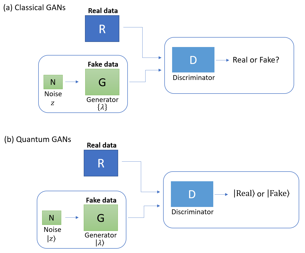
We first provide a high-level overview of the GAN architecture (Goodfellow et al., 2014). We suppose that the real-world data comes from some fixed distribution , generated by some (potentially complex and unknown) process . The generator – parameterized by a vector of real-valued parameters – takes as input an unstructured random variable (typically drawn from a normal or uniform distribution). G transforms this noise source into data samples , creating the generator distribution . In the ideal case of a perfectly trained generator , the discriminator would not be able to decide whether a given sample came from or from . Therefore, the task of training corresponds to the task of maximizing the probability that misclassifies a generated sample as an element of the real data. On the other hand, the discriminator – parameterized by a vector of real-valued parameters – takes as input either real data examples or fake data samples . D’s goal is to discriminate between these two classes, outputting a binary random variable. Training thus corresponds to maximizing the probability of successfully classifying real data, while minimizing the probability of misclassifying fake data.
We will formalize QuGANs as a quantum generalization of conditional GANs (Mirza and Osindero, 2014). Conditional GANs generate samples from a conditional distribution (conditioned on labels ), rather than the unconditional distribution of vanilla GANs. Conditional GANs reduce to vanilla GANs in the case where the label is uninformative about the data, i.e., for all and . A possible motivation for using the conditional approach comes from performing quantum chemistry calculations on quantum computers. For example, one could have a list of VQE state preparations for molecules, labeled by their physical properties. A well-trained QuGAN could produce new molecular states which also have the same properties but were not in the original dataset. In another context, a QuGAN could be used to compress time evolution gate sequences (Kivlichan et al., 2018) for different time steps to use in larger quantum simulations.
II.1.2 Quantum GANs
We will now generalize these ideas to the quantum setting. In Figure 1, we highlight the structural similarities of classical and quantum GANs.
For the quantum case, suppose we are given a data source which, given a label , outputs a density matrix into a register containing subsystems, i.e.,
| (1) |
The general aim of training a GAN is to find a generator which mimics the real data source . In the quantum case, we define to be a variational quantum circuit whose gates are parametrized by a vector . The generator takes as input the label and an additional state , and produces a quantum state,
| (2) |
where is output on a register containing subsystems, similar to the real data.
The role of the extra input state is two-fold. On one hand, it can be seen as a source of unstructured noise which provides entropy within the distribution of generated data. For instance, we could have a generator which is unitary, producing a fixed state for each and . By allowing the input to randomly fluctuate, we can create more than one output state for each label. On the other hand, the variable can serve as a control for the generator. By tuning , we can transform the output state prepared by the generator, varying properties of the generated data which are not captured by the labels . During training, the generator should learn to encode the most important intra-label factors of variation with . While the first role could have been accomplished via coupling the generator to a bath, the second role requires to be under our control, even if we endow it with no explicit structure during training.
As in the classical case, the training signal of the generator is provided by a discriminator , made up of separate quantum circuit parametrized by a vector . The task of is to determine whether a given input state was created by the real data source or the generator , whereas the task of is to fool into accepting its output as being real. If the input was created by , then should output in its output register, otherwise it should output . The discriminator is also allowed to do operations on an internal workspace. In order to force to respect the supplied labels, the discriminator is also given an unaltered copy of the label .
The optimization objective for QuGAN training can be formalized as the adversarial task , or:
| (3) |
For classical GANs, the optimization task is traditionally defined with log-likelihood functions but it is more convenient to define a cost function linear in the output probabilities of in the quantum case since we want to optimize a function which is linear in some expectation value. Since the logarithmic function is convex, the optimal points are the same. Finally, for simplicity, the formula above assumes that the labels are countable, with cardinality , though this could be relaxed.
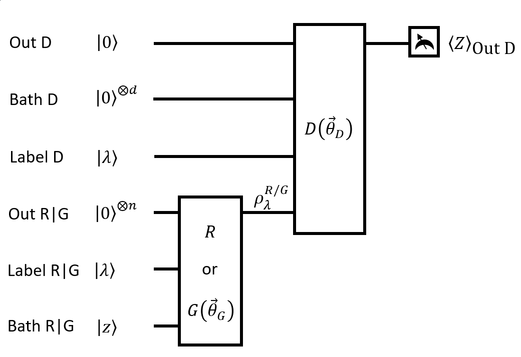
The heuristic of the algorithm is illustrated in Figure 2, where the quantum circuit is divided into 6 operationally defined registers. The real source and the generator are given a label in the -subsystem register Label R|G, an initial blank state on the -subsystem register Out R|G and a noise vector on the -subsystem register Bath R|G. In this work, we assume that is a purified unitary operation on subsystems. In general, the real source may be a physical device entangled with an unknown number of environmental degrees of freedom , with . With no loss of generality, we can assume that the Bath R|G register is initialized in the reference state when the source is as the entropy can be provided by the environment. We assume that the discriminator does not have access to the Bath R|G register.
outputs its answer or on the register Out D. It is given the state of the source through register Out R|G. The workspace of the discriminator is defined on the -subsystem register Bath D and a reference copy of the label is fed through the -subsystem register Label D. Finally, the expectation value of the operator
| (4) |
on the Out D register is proportional to and can be used to define the optimization problem (3) in a fully quantum mechanical setting.
II.1.3 The quantum cost function
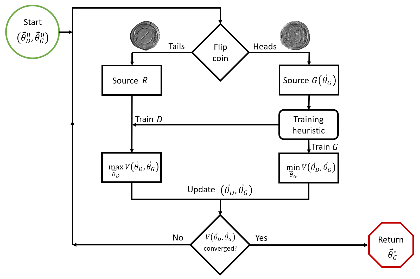
We will follow the flow of the training process as illustrated in Figure 3 to rewrite and analyze the quantum version of the cost function (3). At the beginning of the algorithm, the discriminator and the generator are respectively initialized by the (arbitrary) parameters . The quantum computer of Figure 2 is initialized in the state
| (5) |
If only either or were systematically fed into , the optimal strategy of the latter to maximize the cost function (3) would be to trivially output a constant answer, which is not desirable. In order to make sure that cannot rely on the statistics of the choice of the source to determine its answer, the choice of or can be made by the toss of a fair coin. The unitary operations corresponding to the sources and acting on the whole quantum computer have the respective form
| (6) |
After the chosen source has been applied, the quantum computer is in the corresponding state
| (7) |
The unitary operation defining the discriminator has the form
| (8) |
such that the state of the quantum computer when follows is given by
| (9) |
and the state when is applied after is
| (10) |
The cost function (3) can then be written in the quantum formalism as
| (11) |
where both parts depend on and only the second part depends on , as in the classical case (Goodfellow et al., 2014). Here the angle parametrizes the bias of the coin used in Figure 3 since the probability that or is used as a source is not explicitly constrained in (3). Assuming a fair coin , the quantum optimization problem has the final form
| (12) |
II.1.4 Limit cases of the training
The probability that successfully assigns the correct label to and is given by the cost function . In what follows we will refer to this probability as . In the ideal case where , G perfectly reproduces the statistics of the data source, cannot distinguish (Buhrman et al., 2001; Aaronson, 2007) between and , and . At this point the training is finished as cannot improve its strategy and all gradients vanish:
| (14) |
During the training, is bounded by the purity function
| (15) |
such that the performance of the discriminator is
| (16) |
The purity function is itself bounded by the nature of . If we define as being the minimal eigenvalue of , then
| (17) |
where the upper bound corresponds to the purity of .
It is possible to train the circuit of Figure 2 by evaluating gradients from a numerical finite difference method. This requires sampling many points around each to estimate the gradient of (12). In the following section, we will show how gradients can be evaluated directly on a quantum computer and explicitly construct the circuits to optimize (12).
II.2 Quantum gradients
A key element of GANs is that the generator can be optimized by using gradient signals obtained from the discriminator. Thus, in addition to quantum circuits for and , we would also like to have quantum circuits which can compute the required gradients. Given access to these quantum gradients, model parameters can be updated via gradient descent on a classical computer. We introduce some notation useful to define gradient extraction on a quantum computer (Knill and Laflamme, 1998; Ortiz et al., 2002; Romero et al., 2017; Farhi and Neven, 2018; Schuld and Killoran, 2018; Schuld et al., 2018). In order to present a specific circuit setup, from here onwards we fix that the subsystems of our quantum computer are qubits. We also note that, in addition to the particular setup we use here, there can be other approaches for using a quantum computer to compute gradients of quantum circuits. A unitary transformation parametrized by a vector with components is denoted
| (18) |
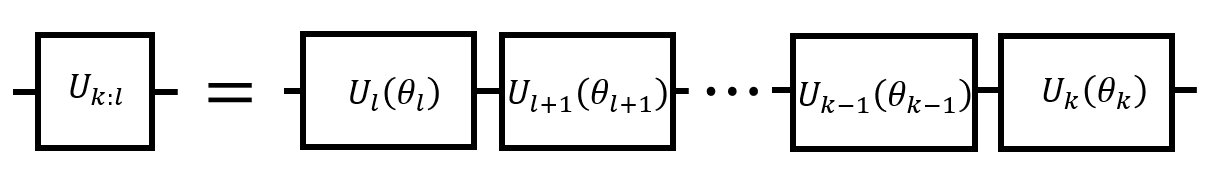
where is the time-ordering operator. It is convenient to introduce the ordered notation (Machnes et al., 2011)
| (19) |
which can also be represented in a quantum circuit notation as shown in Figure 4. In the same fashion, the anti-ordered notation has the form
| (20) |
where is the anti-time ordering operator. It follows that we can generally denote and .
Assuming each element is generated by a Hamiltonian , an individual gate has the form
| (21) |
such that . The derivative of gate with respect to parameter is given by
| (22) |
Using the chain rule, we find that
| (23) |
If we define an initial state on qubits as , the expectation value of an observable evaluated for parameters is given by
| (24) |
The gradient with respect to a parameter is then given by
| (25) |
where is the commutator.
At this point it is convenient to introduce some canonical quantum gates (Nielsen and Chuang, 2009). Specifically, the Hadamard gate is defined as , the NOT gate as and . It is also useful to define the single-qubit gate as
| (26) |
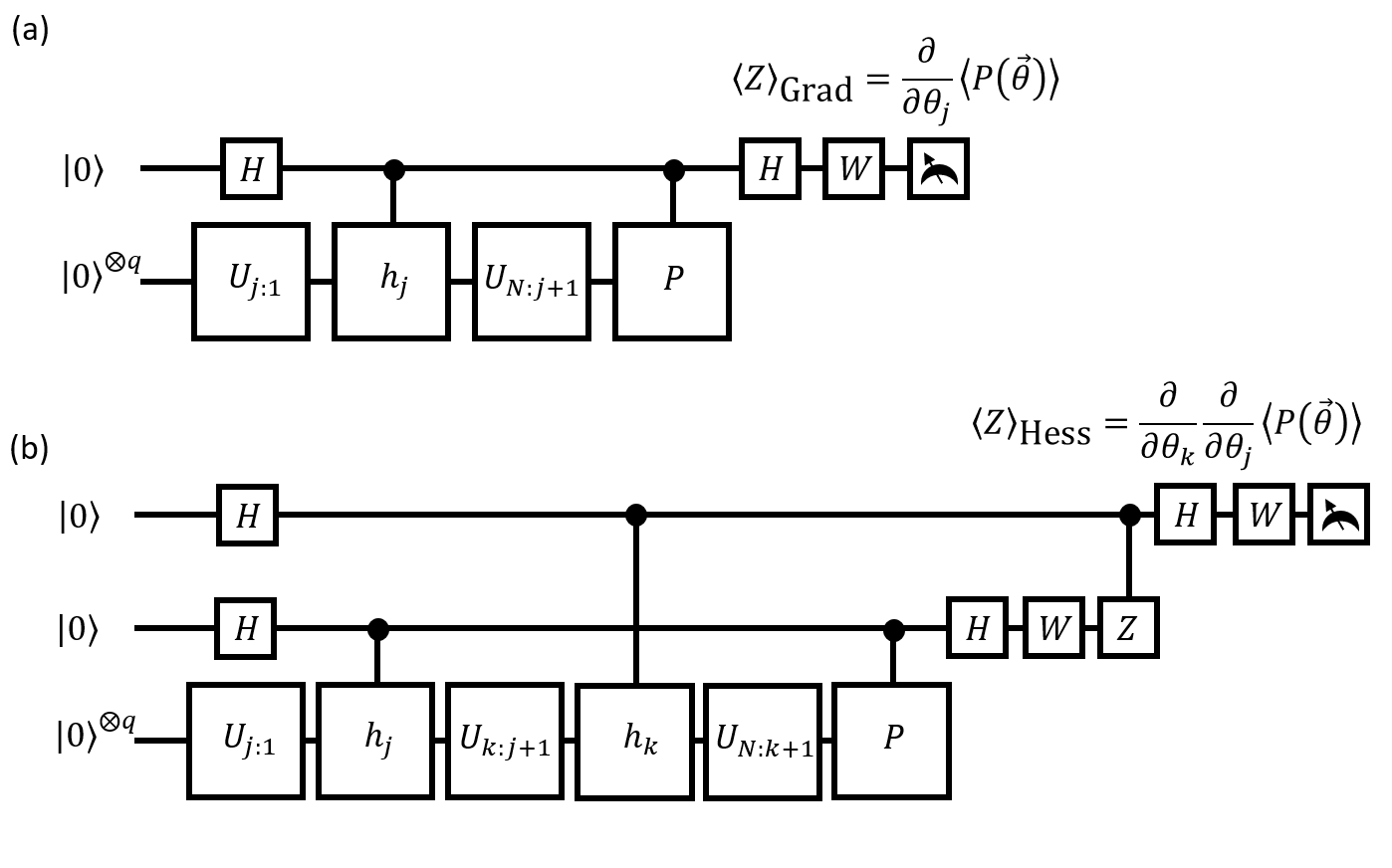
As shown in Figure 5 (a), the gradient of a parametrized quantum circuit can be sampled from the expectation value of an ancillary qubit such that
| (27) |
Note that this requires the ability to perform control gates for the Hamiltonians and measurement operator . Similarly, using the fact that the Hessian is the gradient of a gradient, we show how the Hessian can be measured in Figure 5 (b), such that the output is
| (28) |
II.3 Using quantum gradients to train QuGANs
We now have all the elements required to evaluate the gradients of (13) directly on a quantum computer. The operator from Section II.2 corresponds to the operator of (4) when computing gradients. The parametrized discriminator and generator can be decomposed into respectively and gates, such that
| (29) |
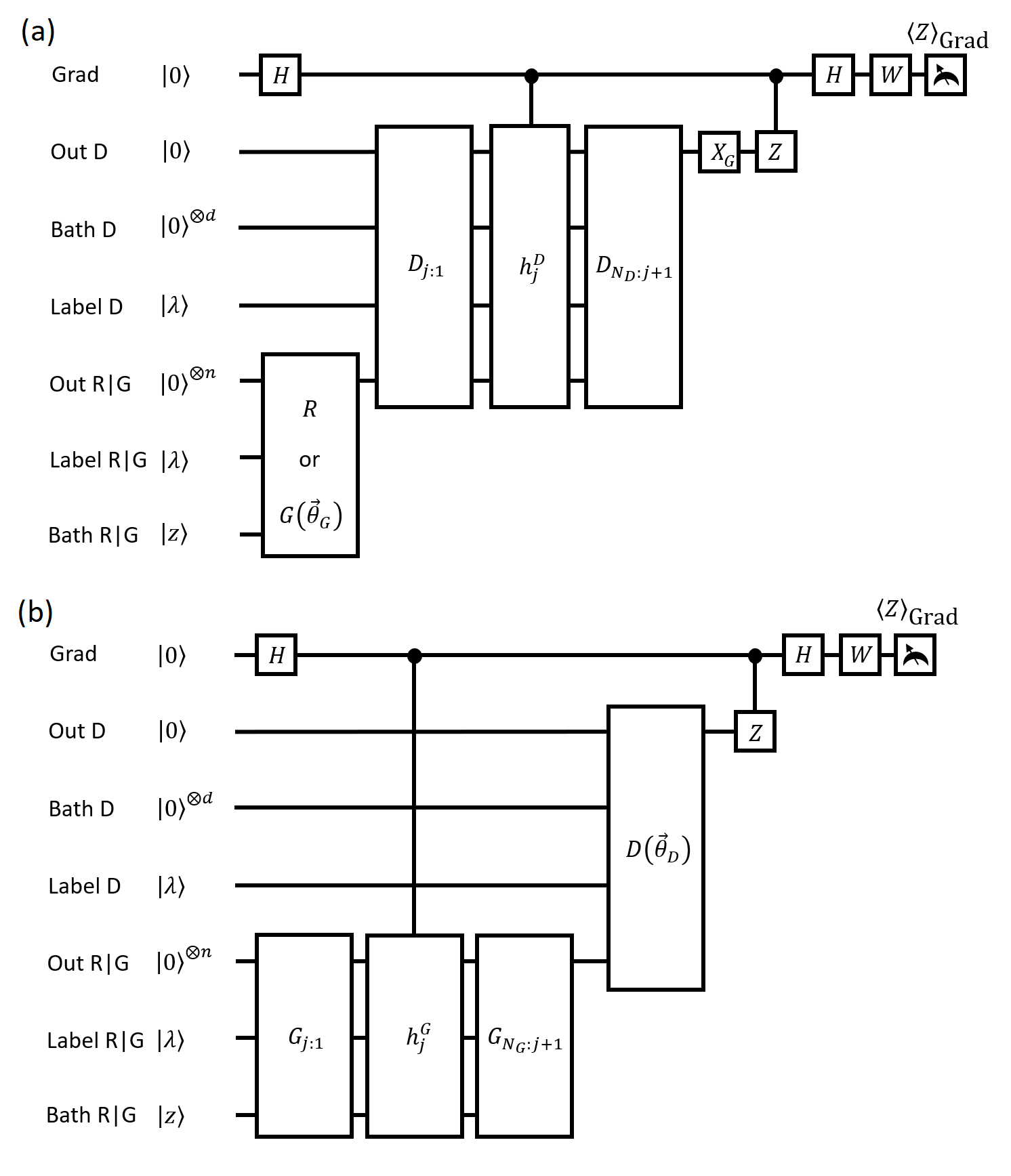
In order to measure gradients, we introduce a single-qubit register Grad. It follows that all elements of the gradient of the discriminator
| (30) |
can be evaluated for each label and sources and by the quantum circuit of Figure 6 (a) with an appropriate gate to account for the sign of the cost function. In the later case, an gate is applied on the Out D register after the discriminator to get the correct sign of the gradient. The circuit that yields the gradient
| (31) |
of the generator for each label is shown in Figure 6 (b). We note that the sign is meant to be the same as the one in (13), such that the generator improves its capability to fool the discriminator. More advanced methods to update the parameters could also leverage the use of quantum Hessians (28).
II.3.1 Improved training heuristics
Training GANs is equivalent to finding the Nash equilibrium of a two-player game. This problem is known to be in the complexity class PPAD which is not expected to be contained in BQP (Fellman and Post, 2010; Li, 2011). Advanced heuristics have been developed to improve the training of classical GANs (Salimans et al., 2016). Namely, it should be straightforward to implement semi-supervised learning in the quantum context by increasing the number of labels to and supplying some labeled examples of generated data. Feature matching should also be possible by truncating the decomposition of when evaluating the gradients of with the circuit of Figure 6 (b). We also assumed that the expectation value of each gradient is evaluated from ensemble averaging; it may also be possible to use Bayesian methods to update the parameters after single-shot measurements (Stenberg and Wilhelm, 2016).
II.4 A practical ansatz
A potentially useful ansatz to parametrize and is shown in Figure 7.
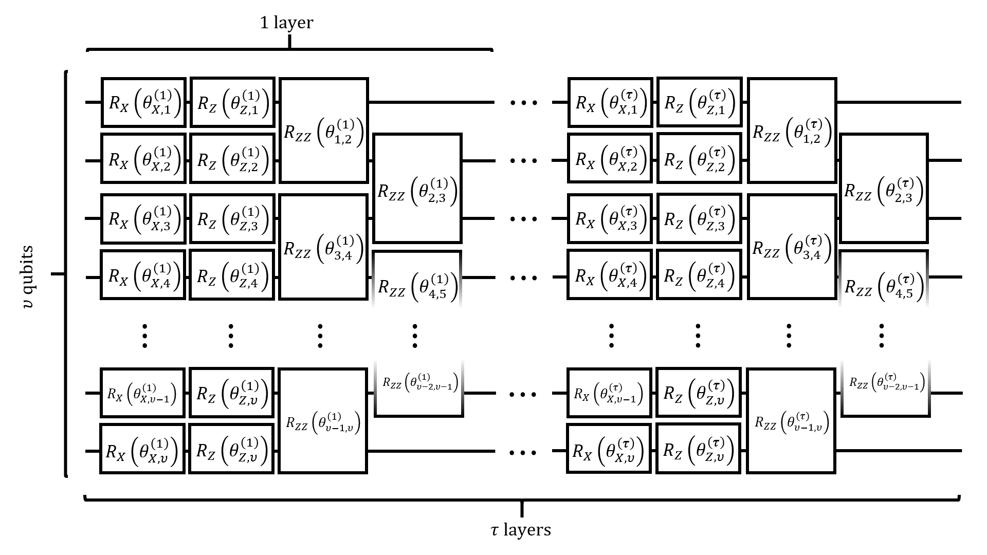
It is universal for quantum computing in the limit of an infinite number of layers . Since the generators of those gates are all simple Pauli operators, it is easy to implement the conditional ’s with CNOTs, CPHASEs and CZZs where the s are between nearest-neighbor qubits. Other types of ansatz may be used depending on the context (Peruzzo et al., 2014; Kandala et al., 2017; Dallaire-Demers et al., 2018; Schuld et al., 2018; Huggins et al., 2018).
II.5 Numerics
We numerically tested ideas in this paper with a simple example involving two labels and . We chose a source such that and . The labels can be encoded in a 1-qubit Label R|G register and the Out R|G register only requires 1 qubit. Since the labeled distributions are pure we don’t need a Bath R|G register to generate entropy. The expected solution is that should be able to generate a CNOT gate conditioned on the label register. We find that this can be achieved with 2 layers of the ansatz previously introduced. This corresponds to 10 variational parameters in .
The discriminator requires at least 1 qubit for its output Out D, 1 qubit for Label D, and it also operates on the 1-qubit Out R|G register. We find that a Bath D register did not appear to improve convergence of our numerical experiments. Therefore, operates on 3 qubits, and we found that 4 layers of the ansatz of section II.4 were sufficient to train the QuGAN. This yields 32 parameters in for a total of 42. With the qubit of register Grad, the algorithm operates on a total of 5 qubits.
Training GANs is a delicate art. To keep this proof-of-principle simple we chose not to use any advanced training heuristic. We trained the QuGAN for 10,000 gradient steps of the update rule (13). The learning rate exponentially decreases from 10 to for the first 4,000 steps and remains constant at the latter value for the remaining 6,000 steps. The generator is only updated once for every 100 steps of with a learning rate .
As shown in Figure 8, the generator has been properly trained at the end of the algorithm, as the cross-entropy
| (32) |
quickly converges to zero. We also plotted the components of the cost function defined as
| (33) |
such that . At the beginning of the training sequence, the parameters are chosen randomly. In order to provide a reliable training signal for , the gradients are amplified by a large learning rate to quickly train . The generator initially produces a decent state for the label but fails to produce a good state for the label. The training of the discriminator appears successful since is typically larger than and learns to differentiate the data produced by from the data produced by . Updating the generator less often than the discriminator provides a trade-off between a fast training of and a good training signal. After a few tens of training steps of (which corresponds to a few thousand training cycles of ) the cross-entropy between the real and the generated data starts to converge to zero as the generator creates better samples. In this case, cannot differentiate and as approaches its equilibrium value of . The final strategy of is to designate all data as real, yielding and .

III Conclusion
Quantum machine learning is likely to be one of the first general-purpose applications of near-term quantum devices. Here we showed how generative models can be trained on quantum computers. We have reformulated the optimization problem of GANs in the quantum formalism, yielding QuGANs. We have shown how the cost function can be optimized by directly evaluating the gradients with a quantum processor. We provided a simple universal qubit ansatz which constrains the set of additional quantum resources required to evaluate the gradients. Finally, we showed that QuGANs can be trained in practice by performing a simple numerical experiment.
It is expected that QuGANs will have a more versatile representation power than their classical counterpart. For example, one can speculate that a large enough QuGAN could learn to generate encrypted data labeled by RSA public encryption keys since quantum computers have the capacity to perform Shor factoring (Shor, 1997) and hence decryption. In that case, the optimal generator would learn a statistical model of the unencrypted data for each key and encrypt with the label. Other classical cryptographic systems (such as elliptic curve) could also be vulnerable to this type of attack. In this work, we have explored the practical issues of QuGANs, namely, explicit quantum circuits for the generator and discriminator, as well as quantum methods for computing the gradients of these circuits. A more general analysis of the theoretical concepts of quantum adversarial learning can be found in the companion paper Lloyd and Weedbrook (2018).
Acknowledgements.
We thank Seth Lloyd and Christian Weedbrook for their insightful advices. This works was made possible by ample supplies of Tim Horton’s coffee.References
- LeCun et al. (2015) Y. LeCun, Y. Bengio, and G. Hinton, Nature 521, 436 (2015).
- Goodfellow et al. (2016) I. Goodfellow, Y. Bengio, and A. Courville, Deep Learning (Adaptive Computation and Machine Learning series) (The MIT Press, 2016).
- Deng (2014) L. Deng, Foundations and Trends in Signal Processing 7, 197 (2014).
- Goodfellow et al. (2014) I. J. Goodfellow, J. Pouget-Abadie, M. Mirza, B. Xu, D. Warde-Farley, S. Ozair, A. Courville, and Y. Bengio, in Proceedings of the 27th International Conference on Neural Information Processing Systems-Volume 2 (MIT Press, 2014) pp. 2672–2680.
- Salimans et al. (2016) T. Salimans, I. Goodfellow, W. Zaremba, V. Cheung, A. Radford, and X. Chen, ArXiv e-prints (2016), arXiv:1606.03498 [cs.LG] .
- Creswell et al. (2018) A. Creswell, T. White, V. Dumoulin, K. Arulkumaran, B. Sengupta, and A. A. Bharath, IEEE Signal Processing Magazine 35, 53 (2018).
- Zhu et al. (2016) J.-Y. Zhu, P. Krähenbühl, E. Shechtman, and A. A. Efros, in European Conference on Computer Vision (Springer, 2016) pp. 597–613.
- Ledig et al. (2016) C. Ledig, L. Theis, F. Huszar, J. Caballero, A. Cunningham, A. Acosta, A. Aitken, A. Tejani, J. Totz, Z. Wang, and W. Shi, ArXiv e-prints (2016), arXiv:1609.04802 [cs.CV] .
- Isola et al. (2016) P. Isola, J.-Y. Zhu, T. Zhou, and A. A. Efros, ArXiv e-prints (2016), arXiv:1611.07004 [cs.CV] .
- Choy et al. (2016) C. B. Choy, D. Xu, J. Gwak, K. Chen, and S. Savarese, in European Conference on Computer Vision (Springer, 2016) pp. 628–644.
- Gulrajani et al. (2017) I. Gulrajani, F. Ahmed, M. Arjovsky, V. Dumoulin, and A. C. Courville, in Advances in Neural Information Processing Systems (2017) pp. 5769–5779.
- Kadurin et al. (2017) A. Kadurin, S. Nikolenko, K. Khrabrov, A. Aliper, and A. Zhavoronkov, Molecular pharmaceutics 14, 3098 (2017).
- Killoran et al. (2017) N. Killoran, L. J. Lee, A. Delong, D. Duvenaud, and B. J. Frey, ArXiv e-prints (2017), arXiv:1712.06148 [cs.LG] .
- de Oliveira et al. (2017) L. de Oliveira, M. Paganini, and B. Nachman, Computing and Software for Big Science 1, 4 (2017).
- Feynman (1982) R. P. Feynman, International Journal of Theoretical Physics 21, 467 (1982).
- Nielsen and Chuang (2009) M. A. Nielsen and I. L. Chuang, Quantum Computation and Quantum Information (Cambridge University Press, 2009).
- Shor (1997) P. W. Shor, SIAM Journal on Computing 26, 1484 (1997).
- Preskill (2018) J. Preskill, ArXiv e-prints (2018), arXiv:1801.00862 [quant-ph] .
- Peruzzo et al. (2014) A. Peruzzo, J. McClean, P. Shadbolt, M.-H. Yung, X.-Q. Zhou, P. J. Love, A. Aspuru-Guzik, and J. L. O’Brien, Nature Communications 5, 4213 (2014).
- Kandala et al. (2017) A. Kandala, A. Mezzacapo, K. Temme, M. Takita, M. Brink, J. M. Chow, and J. M. Gambetta, Nature 549, 242 (2017).
- Moll et al. (2017) N. Moll, P. Barkoutsos, L. S. Bishop, J. M. Chow, A. Cross, D. J. Egger, S. Filipp, A. Fuhrer, J. M. Gambetta, M. Ganzhorn, A. Kandala, A. Mezzacapo, P. Müller, W. Riess, G. Salis, J. Smolin, I. Tavernelli, and K. Temme, ArXiv e-prints (2017), arXiv:1710.01022 [quant-ph] .
- Giacomo Guerreschi and Smelyanskiy (2017) G. Giacomo Guerreschi and M. Smelyanskiy, ArXiv e-prints (2017), arXiv:1701.01450 [quant-ph] .
- Dallaire-Demers et al. (2018) P.-L. Dallaire-Demers, J. Romero, L. Veis, S. Sim, and A. Aspuru-Guzik, ArXiv e-prints (2018), arXiv:1801.01053 [quant-ph] .
- Schuld et al. (2014) M. Schuld, I. Sinayskiy, and F. Petruccione, Contemporary Physics 56, 172 (2014).
- Arjovsky et al. (2015) M. Arjovsky, A. Shah, and Y. Bengio, ArXiv e-prints (2015), arXiv:1511.06464 [cs.LG] .
- Romero et al. (2017) J. Romero, J. P. Olson, and A. Aspuru-Guzik, Quantum Science and Technology 2, 045001 (2017).
- Romero et al. (2017) J. Romero, R. Babbush, J. R. McClean, C. Hempel, P. Love, and A. Aspuru-Guzik, ArXiv e-prints (2017), arXiv:1701.02691 [quant-ph] .
- Biamonte et al. (2017) J. Biamonte, P. Wittek, N. Pancotti, P. Rebentrost, N. Wiebe, and S. Lloyd, Nature 549, 195 (2017).
- Cao et al. (2017) Y. Cao, G. Giacomo Guerreschi, and A. Aspuru-Guzik, ArXiv e-prints (2017), arXiv:1711.11240 [quant-ph] .
- Verdon et al. (2017) G. Verdon, M. Broughton, and J. Biamonte, ArXiv e-prints (2017), arXiv:1712.05304 [quant-ph] .
- Otterbach et al. (2017) J. S. Otterbach, R. Manenti, N. Alidoust, A. Bestwick, M. Block, B. Bloom, S. Caldwell, N. Didier, E. Schuyler Fried, S. Hong, P. Karalekas, C. B. Osborn, A. Papageorge, E. C. Peterson, G. Prawiroatmodjo, N. Rubin, C. A. Ryan, D. Scarabelli, M. Scheer, E. A. Sete, P. Sivarajah, R. S. Smith, A. Staley, N. Tezak, W. J. Zeng, A. Hudson, B. R. Johnson, M. Reagor, M. P. da Silva, and C. Rigetti, ArXiv e-prints (2017), arXiv:1712.05771 [quant-ph] .
- Schuld and Killoran (2018) M. Schuld and N. Killoran, ArXiv e-prints (2018), arXiv:1803.07128 [quant-ph] .
- Schuld et al. (2018) M. Schuld, A. Bocharov, K. Svore, and N. Wiebe, ArXiv e-prints (2018), arXiv:1804.00633 [quant-ph] .
- Huggins et al. (2018) W. Huggins, P. Patel, K. B. Whaley, and E. Miles Stoudenmire, ArXiv e-prints (2018), arXiv:1803.11537 [quant-ph] .
- Farhi and Neven (2018) E. Farhi and H. Neven, ArXiv e-prints (2018), arXiv:1802.06002 [quant-ph] .
- Mitarai et al. (2018) K. Mitarai, M. Negoro, M. Kitagawa, and K. Fujii, ArXiv e-prints (2018), arXiv:1803.00745 [quant-ph] .
- Lloyd and Weedbrook (2018) S. Lloyd and C. Weedbrook, ArXiv e-prints (2018), arXiv:1804.09139 [quant-ph] .
- Mirza and Osindero (2014) M. Mirza and S. Osindero, ArXiv e-prints (2014), arXiv:1411.1784 [cs.LG] .
- Kivlichan et al. (2018) I. D. Kivlichan, J. McClean, N. Wiebe, C. Gidney, A. Aspuru-Guzik, G. K.-L. Chan, and R. Babbush, Physical Review Letters 120, 110501 (2018).
- Buhrman et al. (2001) H. Buhrman, R. Cleve, J. Watrous, and R. de Wolf, Physical Review Letters 87, 167902 (2001).
- Aaronson (2007) S. Aaronson, Proceedings of the Royal Society A: Mathematical, Physical and Engineering Sciences 463, 3089 (2007).
- Knill and Laflamme (1998) E. Knill and R. Laflamme, Physical Review Letters 81, 5672 (1998).
- Ortiz et al. (2002) G. Ortiz, J. Gubernatis, E. Knill, and R. Laflamme, Computer Physics Communications 146, 302 (2002).
- Machnes et al. (2011) S. Machnes, U. Sander, S. J. Glaser, P. de Fouquières, A. Gruslys, S. Schirmer, and T. Schulte-Herbrüggen, Physical Review A 84, 022305 (2011).
- Fellman and Post (2010) P. V. Fellman and J. V. Post, in Unifying Themes in Complex Systems (Springer Berlin Heidelberg, 2010) pp. 454–461.
- Li (2011) Y. D. Li, ArXiv e-prints (2011), arXiv:1108.0223 [cs.CC] .
- Stenberg and Wilhelm (2016) M. P. V. Stenberg and F. K. Wilhelm, Physical Review A 94, 052119 (2016).