X-Ray Properties of AGN in Brightest Cluster Galaxies. I. A Systematic Study of the Chandra Archive in the $0.2<z<0.3$ and $0.55<z<0.75$ Redshift Range

Abstract

We present a search for nuclear X-ray emission in the brightest cluster galaxies (BCGs) of a sample of groups and clusters of galaxies extracted from the Chandra archive. The exquisite angular resolution of Chandra allows us to obtain robust photometry at the position of the BCG, and to firmly identify unresolved X-ray emission when present, thanks to an accurate characterization of the extended emission at the BCG position. We consider two redshift bins ($0.2<z<0.3$ and $0.55<z<0.75$) and analyze all the clusters observed by Chandra with exposure time larger than 20 ks. Our samples have 81 BCGs in 73 clusters and 51 BCGs in 49 clusters in the low- and high-redshift bin, respectively. X-ray emission in the soft (0.5-2 keV) or hard (2-7 keV) band is detected only in 14 and 9 BCGs ($\sim 18$% of the total samples), respectively. The X-ray photometry shows that at least half of the BCGs have a high hardness ratio, compatible with significant intrinsic absorption. This is confirmed by the spectral analysis with a power-law model plus intrinsic absorption. We compute the fraction of X-ray bright BCGs above a given hard X-ray luminosity, considering only sources with positive photometry in the hard band (12/5 sources in the low/high-z sample). In the $0.2<z<0.3$ interval the hard X-ray luminosity ranges from $10^{42}$ to $7\times 10^{43}$ erg s^-1, with most sources found below $10^{43}$ erg s^-1. In the $0.55<z<0.75$ range, we find a similar distribution of luminosities below $\sim 10^{44}$ erg s^-1, plus two very bright sources of a few $10^{45}$ erg s^-1 associated with two radio galaxies. We also find that X-ray luminous BCGs tend to be hosted by cool-core clusters, despite the majority of cool cores do not host nuclear X-ray emission. This work shows that our analysis, when extended to the entire Chandra archive, can provide a sizable number of sources allowing us to probe the evolution of X-ray AGN in BCGs as a function of the cosmic epochs.

1 Introduction

Brightest cluster galaxies (BCGs) are defined as galaxies that spend most of their life at the bottom of the potential wells of massive dark matter halos. This particular location favors accretion from satellite galaxies or from gas cooling out of the hot phase of the intracluster medium (ICM). In turn, cooling gas may feed several star formation episodes (e.g., Bonaventura et al., 2017) or mass growth of the central super massive black hole (SMBH). Therefore, their evolution is directly linked to the dynamical history of the host cluster and to the cycle of baryons in cluster cores. For these reasons, BCGs are the largest and most luminous ones among the cluster galaxy population. Due to the hierarchical process of structure formation, in dynamically young clusters or major mergers there may be more than one BCG, so that BCGs may not be unambiguously defined as the brightest galaxies. In addition, in such dynamically disturbed halos, their position may not coincide with the center of the X-ray emission (see Rossetti et al., 2016). Despite the intrinsic difficulty in defining a unique BCG at any epoch during the lifetime of a virialized massive halo, in most of the cases, BCGs are by far the most luminous galaxies in the optical band, and their position is almost coincident with the peak of the X-ray brightness, with a typical displacement of less than 10 kpc (Katayama et al., 2003). This is a typical case in relaxed, cool-core cluster, where their identification is straightforward. Alternatively, off-centered or multiple BCGs (reported for a fraction ranging from 5% to 15%, see Crawford et al., 1999; Hogan et al., 2015) are often associated with signatures of ongoing or recent major mergers.

An important property of BCGs is the ubiquitous presence of significant nuclear radio emission. Best et al. (2005, 2007) showed that BCGs are more likely to host a radio-loud AGN by a factor of several with respect to normal ellipticals, although only 20-30% of the BCGs can be defined radio-loud AGN. The likely cause of this behavior is the increasing amount of fueling surrounding the BCG in the form of cold gas cooling out the hot phase. Indeed, the dependence on the SMBH mass of the radio-loud AGN fraction (Best et al., 2005) mirrors that of the cooling rate from the hot halos. Recently, ¹³CO line emission from molecular gas has been detected in BCGs (see, e.g., Vantyghem et al., 2017).

The origin of the cold gas is problematic, to say the least. Observationally, pure isobaric cooling flows (Fabian, 1994) are not observed, and X-ray spectra indicate that they must be suppressed in flux at least by a factor of 10-100, in particular in the soft X-rays (e.g., Peterson & Fabian 2006). Since star formation is linked to the cooling gas, BCG star formation rates in the range 1-100 $M_{\odot}yr^{-1}$ are observed to be quenched as well, albeit with large scatter that is due to the temporal delays involved (e.g., Molendi et al. 2016). The thermal structure of the hot gas and the quenched star formation can be reconciled by invoking a plethora of complex phenomena collectively named feedback, where AGN are the most likely feedback agent. The AGN present in the central galaxies can inject mechanical energy through relativistic jets or winds. This energy is most likely thermalized at $r\mathrel{\mathchoice{\lower 2.5pt\vbox{\halign{$\mathsurround 0pt\displaystyle\hfil#\hfil$\cr>\crcr\sim\crcr}}}{\lower 2.5pt\vbox{\halign{$\mathsurround 0pt\textstyle\hfil#\hfil$\cr>\crcr\sim\crcr}}}{\lower 2.5pt\vbox{\halign{$\mathsurround 0pt\scriptstyle\hfil#\hfil$\cr>\crcr\sim\crcr}}}{\lower 2.5pt\vbox{\halign{$\mathsurround 0pt\scriptscriptstyle\hfil#\hfil$\cr>\crcr\sim\crcr}}}}10$ - 100 kpc via buoyant hot bubbles, weak shocks, and turbulence (e.g., Gaspari et al. 2013a; Barai et al. 2016). While the macro imprints of AGN feedback can be resolved by current X-ray telescopes, the actual micro carrier of kinetic energy is still debated. The radio electron synchrotron power of relativistic jets is typically over 100 times lower than the total cavity power (McNamara & Nulsen 2012); the Fermi telescope has not detected any substantial gamma-ray emission within bubbles, hence excluding relativistic protons; in addition, several (‘ghost’) cavities have been found to be devoid of radio emission (see Bîrzan et al., 2004). Another source of feedback can be massive sub-relativistic outflows, typically with a wider opening angle compared to jets, which are able to entrain the background gas along the path. Detections of multiphase AGN outflows are booming during the past few years (e.g., Tombesi et al. 2013; Russell et al. 2014; Combes 2015; Feruglio et al. 2015; Morganti 2015). Overall, the radio power can be a tracer of feedback, although there are also other mechanical injection channels that are not necessarily associated with an increase of nuclear radio power. It is thus best to refer to this mode of feedback as the mechanical mode (which includes both relativistic jets and sub-relativistic outflows) instead of as the radio mode.

In recent years, a detailed picture of AGN feeding in massive halos has emerged (e.g., Gaspari et al. 2013b; Voit et al. 2015b, a). According to this picture, warm filaments and cold clouds are expected to condense out of the hot gaseous halo of the massive galaxy, group, or cluster in a multiphase condensation cascade and rain toward the central AGN. Inelastic collisions promote angular momentum cancellation, boosting the accretion rate and thus increasing the nuclear AGN power. This mechanism is known as chaotic cold accretion (CCA). The CCA feeding triggers the feedback via AGN jets or outflows in a tight self-regulated loop (see Gaspari et al., 2017).

This is a promising mechanism, since, on the basis of the ubiquitous observations of a quenched cooling rate in cool cores, the mechanical mode of AGN feedback is expected to be tightly self-regulated in most – if not all – BCGs (e.g., Sun 2009). This mode is often associated with radiatively inefficient accretion on AGN (Fabian, 2012). However, a fraction of BCGs also shows substantial X-ray emission, suggesting the coexistence of a radiatively efficient accretion disk or momentarily boosted rain near the inner SMBH hosted by the BCG. The X-ray properties of BCGs have been systematically investigated by Russell et al. (2013) in a low-redshift sample, to explore the relation between nuclear X-ray emission and AGN cavity power. They found that half of their sample has detectable unresolved X-ray emission. They estimated the accretion rate from the cavity power (assuming some efficiency), finding that the nuclear radiation exceeds the mechanical power when the mean accretion rate is above a few percent of the Eddington rate ($\sim 22\,M_{\odot}$ yr^-1 for a $10^{9}\,M_{\odot}$ SMBH), marking the transition from radiatively inefficient AGN to quasars, as expected from the fundamental plane of black hole activity (Merloni et al., 2003). As before, they remarked that cold gas fueling is the likely source of accretion (e.g., Nulsen, 1986; Pizzolato & Soker, 2005; McNamara et al., 2016). Hlavacek-Larrondo et al. (2013a) investigated the nuclear X-ray emission of BCGs in bright X-ray clusters with clear X-ray cavities. They found a strong evolution in their nuclear X-ray luminosity, at least by a factor of $\sim$ 10 in the $0<z<0.6$ redshift range, speculating that the transition from mechanically dominated AGN to quasars occurs at high redshift for the majority of the massive cluster population.

The analysis of both Russell et al. (2013) and Hlavacek-Larrondo et al. (2013a) are based on a sample of BCGs whose host cluster shows large X-ray cavities in the ICM. The presence of cavities, together with a nuclear radio power, allows one to estimate the mean accretion rate onto each galaxy on a time scale of $\sim$ $10^{8}$ years. Here we relax this requirement to extend the investigation of unresolved X-ray emission from BCGs to any virialized halo, defined by the presence of diffuse emission from its ICM. Clearly, with these selection criteria, we are dominated by halos with low X-ray surface brightness, and therefore we are not able to search for X-ray cavities. Our long-term plan is to collect enough archival, multiwavelength data to use SMBH mass estimate and properties of the environment (such as mass of the host halo, cool-core strength, presence of cavities, and dynamical state of the halo) with the final goal of exploring the origin of the X-ray emission, the accretion regime in BCGs at different epochs and environments, and the origin of the feeding gas and obscuring material around the SMBH. In this first paper of a series, our immediate science goal is to assess our capability of tracing the X-ray properties of the BCGs across the wide range of groups and clusters of galaxies currently available in the Chandra archive. In particular, we focus on the 2-10 keV nuclear luminosity of BCGs at two different cosmic epochs. Only the exquisite angular resolution of Chandra data allows us to unambiguously identify the presence of unresolved X-ray emission embedded in the much brighter thermal ICM emission, which must be efficiently modeled and subtracted.

The paper is organized as follows. In §2 we describe the sample selection. In §3 we describe the data reduction and analysis, and in §4 we provide the results of the X-ray properties of BCGs and the correlation between X-ray and radio nuclear emission, and the link with the cool-core strength. In §5 we discuss the possible implications for AGN feeding and feedback that can be obtained from our study. Finally, in §6 we summarize our conclusions. Throughout the paper, we adopt the seven-year WMAP cosmology ($\Omega_{\Lambda}=0.73$, $\Omega_{m}=0.27$, and $H_{0}=70.4$ km s^-1 Mpc^-1 (Komatsu et al., 2011). Quoted error bars correspond to a 1 $\sigma$ confidence level unless noted otherwise.

2 Sample definition

2.1 X-Ray Data Selection

To achieve our science goals, we aim at considering both cool-core and non-cool-core clusters, with no preselection based on cluster properties, except for the firm detection of extended ICM thermal emission, which is the unambiguous signature of a virialized halo. Therefore we initially consider the entire Chandra ACIS archival observations listed under the category ”clusters of galaxies”. This maximally inclusive selection simply aims at collecting the largest number of BCGs imaged with the best angular resolution. In fact, the vast majority of Chandra ACIS aimpoints coincide with the cluster center, ensuring the best angular resolution at the BCG position and therefore allowing us to identify unresolved emission above the level of the surrounding ICM. This aspect is key to our research strategy, since the capability of detecting unresolved emission embedded in the ICM is rapidly disappearing as the point spread function is degraded as a function of the off-axis angle. We are aware that the large source list initially selected in this way does not constitute a complete sample. In addition, this choice does not allow any control on possible selection bias. On the other hand, due to the intrinsic differences among cluster samples with difference selection (see Rossetti et al., 2017, for X-ray and Sunyaec-Zel’dovich, SZ, selected clusters samples), a complete and unbiased sample of virialized halos will necessarily be a mix of clusters selected with different criteria. This consideration pushes us to exploit the entire Chandra archive with no further restrictions, as an acceptable proxy to an unbiased cluster sample. Our plan is to test our strategy and eventually extract well-defined subsamples from the main parent sample after completing the collection of useful X-ray data.

Since we wish to explore the X-ray properties of BCGs as a function of the cosmic epoch, we first apply our method in two redshift bins that include a sufficiently large number of clusters (i.e., at least 50 in each of them). When the same target has multiple exposures, we decide to choose the ObsIDs with the largest total exposure between ACIS-I and ACIS-S, and avoid combining the two detectors for simplicity. In addition, we discard short observations if taken in an observing mode different from the bulk of the observations. In this work, aiming essentially in testing our strategy, we choose to analyze all the groups and clusters observed with total exposure time $t_{exp}>20$ ks to ensure a good characterization of the extended ICM emission, and eventually perform a spatially resolved analysis of the surrounding ICM whenever possible.

In defining the low-redshift bin, we prefer to avoid nearby clusters, so that we can always sample the background from the ICM-free regions around the clusters in the $8\times 8$ arcmin field of view (corresponding to one Chandra ACIS CCD). We find that the choice $0.2<z<0.3$ allows us to obtain a sufficiently large sample and also have a few sources overlapping with the sample of Russell et al. (2013) for a direct comparison. We choose the range $0.55<z<0.75$ for the high-redshift bin to include a sizable number of clusters. Moreover, with these choices, we probe a redshift range comparable to that explored by Hlavacek-Larrondo et al. (2013a). We have 73 and 49 clusters in the low- and high- redshift bin, respectively. With this choice we aim at delivering a first investigation of the typical X-ray luminosity of BCGs in virialized halos on a time scale of about 3 Gyr (from $\langle z\rangle=0.65$ to $\langle z\rangle=0.25$), paving the way to an eventual comprehensive study based on the entire Chandra archive.

2.2 BCG Identification

As we discussed in the Introduction, a BCG can be defined as a galaxy that spent a significant part of its life at the center of a large dark matter virialized halo. This opens up the possibility that each group or cluster hosts more than one BCG at a given time. Or, more likely, that at any time, it is possible to identify one or more past-BCGs, and at least one current BCG. A complete BCG identification strategy based on these premises is beyond our reach with present data, and we are necessarily restricted to those galaxies that are currently experiencing their BCG phase. Therefore, we proceed first by identifying the BCG in the optical band among those with a redshift (when available) that is compatible with the cluster redshift, starting our search from the maximum of the cluster X-ray emission. In most cases, we rely on previous identification of the BCG published in the literature. Then, we search for galaxies that have been identified as secondary BCGs in the literature, if any. We do not apply further criteria for the identification of the BCG. Therefore, we also need to collect high-quality multiwavelength data for the same fields selected in the X-ray band. We make use of Hubble Space Telescope (HST) images or other lower quality optical data whenever available. In the worst cases, when there are no records in the literature, or no HST images, we have to rely on the best information we can recover from the NASA Extragalactic Database. In this case, we avoid searching for a secondary BCG.

In detail, we obtain the most accurate position of the nucleus of the BCG in the following way. First, we inspect the X-ray image, and obtain the coordinates at the maximum of the X-ray surface brightness emission, identified with ds9 in the total band (0.5-7 keV) image. In the case of very smooth X-ray emission, we choose the emission-weighted center. We stress that the initial choice of the X-ray center does not affect the final BCG identification, since it is used merely as a starting point. Eventually, we search for HST images within 2 arcmin from the approximate X-ray center. We download an optical image from the HST archive, visually inspect the X-ray and optical images, and finally select the position of the nucleus of the BCG. In addition, we search for the BCG position in the literature from different works to confirm our BCG identification. When no HST data are available, we refer to the literature and/or to the NASA Extragalactic Database, where we search for the 2MASX or SDSS counterpart closest to the X-ray center we preselected. The positional accuracy obtained in this way is always on the order of $\sim$ 1 arcsec, which is sufficient to unambiguously identify the X-ray unresolved emission associated with the BCG, when present. In the cases of clear unresolved X-ray emission associated to the BCG, we slightly refine the center of the extraction region to sample at best the BCG X-ray emission. In all the other cases (no unresolved emission), the typical $\sim 1$ arcsec uncertainty on the position of the BCG nucleus has a negligible impact on the estimation of the upper limit to the BCG X-ray emission.

Figure 1: Upper panels: HST/ACS image (left) and Chandra hard band image (right) of MS 0735.6+7421 at $z=0.216$. The BCG position, taken from the optical image, is shown as a circle with a radius of 1.2”, which corresponds to the X-ray signal extraction region. No unresolved X-ray emission is observed at the BCG position. Lower panels: the same as in the upper panels for SPT-CL J2344-4243 at $z=0.596$ (the Phoenix cluster), which shows a prominent unresolved emission in the hard band.

In the redshift range $0.2<z<0.3$, we have 40 clusters with HST images. Seven clusters show a secondary BCG that may be associate with a minor or comparable mass halo that recently merged with the main cluster. We find a secondary BCG in A2163 (see Maurogordato et al., 2008), AS0592, RXC J1514.9-1523 (Kale et al., 2015), A1682 (Macario et al., 2013), Z5247 (Kale et al., 2015), CL 2341.1+0000 and 1E0657-56 (Clowe et al., 2006), most of which are well-known major mergers where the merging halos can be clearly identified in the X-ray image. In one case (A2465, see Wegner, 2011) we identify two separate X-ray halos belonging to the same superstructure. Therefore we finally consider 81 BCGs out of 73 clusters and groups. The BCG list in the redshift bin $0.2<z<0.3$, with redshift, position, and relevant references, is shown in Table 1.

In the redshift range $0.55<z<0.75$, we have only 20 clusters with HST images. Only 1 cluster is reported to have 3 BCGs (MACS J0025.4-1222, Bradač et al., 2008). Therefore, we finally consider 51 BCGs out of 49 clusters and groups. In the high-redshift sample, some positions are based uniquely on the X-ray centroid (8 cases out of 51), since we are not able to find the identification of the BCG and its position in the literature, nor to do this on the basis of available optical data. However, in all these cases, there are no hints of unresolved X-ray emission from a BCG embedded in the ICM, so this choice does not affect our results as far as the X-ray selection function is concerned. The BCG list in the redshift bin $0.55<z<0.75$, with redshift, BCG position and relevant references, is shown in Table 2.

As an example, we show in Figure 1 two different cases: MS 0735.6+7421 at $z=0.216$ (upper panels) and SPT-CL J2344-4243 at $z=0.596$ (the Phoenix cluster, lower panels). In both cases the position of the BCG is chosen from the HST image. For MS 0735.6+7421 the HST image, on the left, is taken with ACS with the F850LP filter (PI: McNamara). The hard-band Chandra image, on the right, shows no unresolved emission at the center, although MS 0735.6+7421 is one of the most powerful outbursts known to date (McNamara et al., 2005; Gitti et al., 2007). The ICM X-ray emission within the extraction radius, shown as a circle, is used to set the upper limit to a possible sub-threshold unresolved emission in the hard band. In the second case, we use the HST image of the well-known Phoenix cluster (McDonald et al., 2013), taken with WFC3 with the F814W filter (PI: M. McDonald). In this case, the hard-band Chandra image shows strong unresolved emission that dramatically overwhelms the surrounding ICM. The challenge here is to establish well-defined criteria for photometry to treat the many intermediate cases between these two extreme examples.

Table 1: List of BCGs in X-Ray Groups and Clusters Observed by Chandra in the Redshift Range $0.2<z<0.3$ with a Total Exposure of More than 20 ks. The redshift is listed in column 2, while the optical position of the BCG is listed in columns 3 and 4. The dataset used to measure the BCG position is listed in column 5, together with the corresponding reference when available. “HST”, with no reference, means that the positon of the BCG nucleus has been obtained directly from HST images. If a reference is listed first, followed by the name of the counterpart, the position is taken from the literature. In the other cases, we obtain the position from NED (the counterpart name is also listed)

Cluster	$z$	$R.A._{BCG}$	$Decl._{BCG}$	References
G257.34-22.18	0.2026	06:37:14.5	-48:28:23	NED, 2MASX J06371455-4828214
CL 1829.3+6912	0.2030	18:29:05.7	+69:14:06	NED, 2MASX J18290571+6914064 Murgia et al. (2012)
A2163 BCG-1	0.2030	16:15:48.9	-06:08:41	HST, Maurogordato et al. (2008)
A2163 BCG-2	0.2030	16:15:33.5	-06:09:16	HST, Maurogordato et al. (2008)
A963	0.2060	10:17:03.65	+39:02:49.6	HST, Coziol et al. (2009)
RX J0439-0520	0.2080	04:39:02.23	+05:20:44	Kale et al. (2015), 2MASX J04390223+0520443
G286.58-31.25	0.2100	5:31:30.240	-75:11:02.40	Rossetti et al. (2016)
RX J1256.0+2556	0.2120	12:56:02.30	+25:56:36.51	HST
ZW 2701	0.2140	9:52:49.066	+51:53:06.5	HST, Kale et al. (2015), 2MASX J09524915+5153053
RXC J1504-0248	0.2153	15:04:07.49	-02:48:17.45	HST, Kale et al. (2015)
MS 0735.6+7421	0.2160	07:41:44.55	+74:14:37.9	HST
A773	0.2170	9:17:53.416	+51:43:36.95	HST, Kale et al. (2015), 2MASX J09175344+5143379
G256.55-65.69	0.2195	02:25:53.16	-41:54:52.49	NED, LCRS B022355.8-420821 Rossetti et al. (2016)
RXC J0510.7-0801	0.2195	05:10:47.9	-08:01:45.00	Kale et al. (2015), 2MASX J05104786-0801449
MS 1006.0+1202	0.2210	10:08:47.74	+11:47:38.7	NED, 2MASX J10084771+1147379
AS0592 BCG-1	0.2216	6:38:48.605	-53:58:24.37	HST
AS0592 BCG-2	0.2216	6:38:45.15	-53:58:22.11	HST
RXC J1514.9-1523 BCG-1	0.2226	15:14:57.59	-15:23:43.39	Kale et al. (2015), 2MASX J15145772-1523447
RXC J1514.9-1523 BCG-2	0.2226	15:15:03.1	-15:21:53.0	Kale et al. (2015), 2MASX J15150305-1521537
A1763	0.2230	13:35:20.11	+41:00:03.4	HST
PKS 1353-341	0.2230	13:56:05.46	-34:21:10.94	NED, Fomalont et al. (2003)
A1942	0.2240	14:38:21.84	+03:40:13.05	NED, SDSS J143821.32+034013.4
A2261	0.2240	17:22:27.20	+32:07:57.1	HST, Coziol et al. (2009)
1RXS J060313.4+421231	0.2250	06:03:16.7	+42:14:41	HST, NED, 2MASX J06031667+4214416, van Weeren et al. (2012)
A2219	0.2256	16:40:19.8	+46:42:41	HST, Kale et al. (2015), 2MASX J16401981+4642409
CL 0823.2+0425	0.2256	08:25:57.8	+04:14:48.0	NED, 2MASX J08255782+0414480
CL 0107+31	0.2270	01:02:13.5	+31:49:24	NED, 2MASX J01021352+3149243
A2390	0.2280	21:53:36.82	+17:41:43.86	HST, Kale et al. (2015)
A2111	0.2290	15:39:40.5	+34:25:27	NED, Kale et al. (2015), 2MASX J15394049+3425276
A2667	0.2300	23:51:39.40	-26:05:03.3	HST, Coziol et al. (2009)
RX J0439.0+0715	0.2300	04:39:00.5	+07:16:04	HST, Kale et al. (2015), 2MASX J04390053+0716038
RX J0720.8+7109	0.2309	07:20:53.9	+71:08:59.4	HST, NED, 2MASX J07205404+7108586 Mulchaey et al. (2006)
A267	0.2310	01:52:41.98	+01:00:26.4	HST, Coziol et al. (2009)
G342.31-34.90	0.2320	20:23:20.0	-55:36:03	NED, 2MASX J20232005-5536035
A746	0.23225	09:09:18.46	+51:31:27.98	NED, 2MASX J09091846+5131271
A1682 BCG-1	0.2339	13:06:50.1	+46:33:33.1	HST
A1682 BCG-2	0.2339	13:06:45.731	+46:33:30.12	HST
A2146	0.2343	15:56:13.953	+66:20:53.62	HST, Kale et al. (2015), 2MASX J15561395+6620530
RXC J1459.4-1811	0.2357	14:59:28.75	-18:10:45.18	Kale et al. (2015), 2MASX J14592875-1810453
G347.18-27.35	0.2371	19:34:54.4	-50:52:19.2	NED, [GSB2009] J193454.46-505218.5
G264.41+19.48	0.2400	10:00:01.4	-30:16:33.0	NED, 2MASX J10000143-3016331
4C+55.16	0.2411	8:34:54.900	+55:34:21.11	HST, NED WHL J083454.9+553421 Wen et al. (2009)
Z5247 BCG-1	0.24305	12:34:24.100	+09:47:16.00	NED, Kale et al. (2015), 2MASX J12342409+0947157
Z5247 BCG-2	0.24305	12:34:17.567	+9:45:58.16	HST
A2465-1	0.2453	22:39:39.6	-05:43:56	NED, [W2011] J339.91522-05.73214 Wegner (2011)
A2465-2	0.2453	22:39:24.6	-05:47:17	NED, 2MASX J22392454-0547173 Wegner (2011)
A2125	0.2465	15:41:01.98	+66:16:26.56	HST
CL 2089	0.2492	9:00:36.846	+20:53:40.14	HST, Kale et al. (2015) 2MASX J09003684+2053402
RX J2129.6+0005	39.96	21:29:39.952	+00:05:21.15	HST, 2MASX J21293995+0005207
RCS0222+0144	23.33	02:22:40.9	+01:44:42	NED, RCS 01200101288
A2645	0.2510	23:41:17.022	-09:01:11.74	Kale et al. (2015) 2MASX J23411705-0901110
A1835	0.2532	14:01:02.1	+02:52:42.5	HST, Kale et al. (2015) 2MASX J14010204+0252423
A521	0.2533	4:54:06.870	-10:13:24.79	HST, Kale et al. (2015) 2MASX J04540687-1013247
RXC J1023.8-2715	0.2533	10:23:50.21	-27:15:23.99	NED, 2MASX J10235019-2715232
CL 0348	0.2537	1:06:49.40	+01:03:22.66	HST
MS 1455.0+2232	0.2578	14:57:15.04	+22:20:33.60	HST
G337.09-25.97	0.2600	19:14:37.3	-59:28:20	NED, [CB2012] J288.655540-59.472132 Chon & Böhringer (2012)
SL J1204.4-0351	0.2610	12:04:24.3	-03:51:10	NED, 2MASX J12042431-0351096
G171.94-40.65	0.2700	3:12:57.499	+8:22:10.88	HST
A2631	0.2730	23:37:39.76	+0:16:17.0	HST, Coziol et al. (2009)
G294.66-37.02	0.2742	3:03:46.224	-77:52:43.32	Rossetti et al. (2016)
G241.74-30.88	0.2747	05:32:55.6	-37:01:36	NED, [GSB2009] J053255.66-370136.1
RXC J2011.3-572	0.2786	20:11:26.9	-57:25:11	NED, SPT-CL J2011-5725 BCG Guzzo et al. (2009)
A1758	0.2790	13:32:38.4	+50:33:35	HST, Kale et al. (2015) 2MASX J13323845+5033351
G114.33+64.87	0.2810	13:15:05.2	+51:49:03	HST
A697	0.2820	8:42:57.63	+36:22:01	HST
CL 2341.1+0000 BCG-1	0.2826	23:43:40.06	+0:18:21.76	NED, SDSS J234340.07+001822.3
CL 2341.1+0000 BCG-2	0.2826	23:43:35.68	+0:19:50.70	NED, SDSS J234335.66+001951.4
RXC J0232.2-4420	0.2836	2:32:18.57	-44:20:48	HST
RXC J0528.9-3927	0.2839	05:28:52.99	-39:28:18.1	NED, [GSB2009] J052852.99-392818.1 Guzzo et al. (2009)
A611	0.2880	8:00:56.83	+36:03:23.5	HST
3C438	0.2900	21:55:52.25	+38:00:28.35	HST
ZW 3146	0.2906	10:23:39.7	+4:11:10.7	HST, Kale et al. (2015) 2MASX J10233960+0411116
G195.62+44.05	0.29165	9:20:25.756	+30:29:37.74	HST
RX J0437.1+0043	0.2937	04:37:09.5	+0:43:51	Kale et al. (2015), 2MASX J04370955+0043533
A2537	0.2950	23:08:22.3	-02:11:33.2	HST, Kale et al. (2015), 2MASX J23082221-0211315
G262.25-35.36	0.2952	05:16:37.2	-54:30:59	NED, SSTSL2 J051637.18-543059.3 Coziol et al. (2009) Rossetti et al. (2016)
1E0657-56 BCG-1	0.2960	6:58:38.073	-55:57:26.06	HST
1E0657-56 BCG-2	0.2960	6:58:16.089	-55:56:35.33	HST
Abell S295	0.3	2:45:24.812	-53:01:45.56	HST
G292.51+21.98	0.3	12:01:04.953	-39:51:55.14	Rossetti et al. (2016)

Table 2: List of BCGs in X-Ray Groups and Clusters Observed by Chandra in the Redshift Range $0.55<z<0.75$ with a Total Exposure of More than 20 ks. The redshift is listed in column 2, while the optical position of the BCG is listed in columns 3 and 4. The dataset used to measure the BCG position is listed in column 5, together with the corresponding reference when available. “HST” means that the positon of the BCG nucleus has been obtained from HST images and it is found consistent with the corresponding reference. If a reference is listed first, followed by the name of the counterpart, the position is taken from the literature. In the other cases, we obtain the position from NED (the counterpart name is also listed). Finally, in eight cases the position is taken directly from the X-ray surface brightness peak (“X-ray”)

Cluster	$z$	$R.A._{BCG}$	$Decl._{BCG}$	References
ACT J0346-5438	0.55	03:46:55.5	-54:38:55	NED, ACT-CL J0346-5438 BCG
MS 0451.6-0305	0.55	4:54:10.905	-3:00:52.41	HST, Berciano Alba et al. (2010)
V1121+2327	0.562	11:20:56.77	+23:26:27.87	NED, Szabo et al. (2011)
CL 1357+6232	0.5628	13:57:16.8	+62:32:49.6	NED, Szabo et al. (2011)
SPT-CL 2332-5051	0.5707	23:31:51.123	-50:51:53.94	HST, McDonald et al. (2013)
SPT-CL J2148-6116	0.571	21:48:42.720	-61:16:46.20	NED, McDonald et al. (2016)
CL 0216-1747	0.578	2:16:32.632	-17:47:33.17	HST, Perlman et al. (2002)
CL 0521-2530	0.581	05:21:10.5	-25:31:06.5	X-ray, Burenin et al. (2007); Mehrtens et al. (2012)
MS 2053.7-0449	0.583	20:56:21.47	-4:37:50.1	HST, Verdugo et al. (2007)
MACS 0025.4-1222 BCG1	0.584	0:25:33.018	-12:23:16.80	HST, Bradač et al. (2008)
MACS 0025.4-1222 BCG2	0.584	0:25:32.021	-12:23:03.80	HST, Bradač et al. (2008)
MACS 0025.4-1222 BCG3	0.584	0:25:27.380	-12:22:23.00	HST, Bradač et al. (2008)
SDSS J1029+2623	0.584	10:29:12.456	+26:23:31.91	HST, Ota et al. (2012)
CL 0956+4107	0.587	09:56:02.874	+41:07:20.33	NED, Szabo et al. (2011)
MACS 2129.4-0741	0.5889	21:29:26.056	-7:41:28.95	Stern et al. (2010)
ACT J0232-5257	0.59	02:32:42.80	-52:57:22.3	NED, Sifón et al. (2013)
CL 0328-2140	0.59	03:28:13.6	-21:40:19	NED, Liu et al. (2015)
MACS 0647.7+7015	0.5907	6:47:50.23	+70:14:54.01	HST, Stern et al. (2010)
RX J1205	0.5915	12:05:51.372	+44:29:09.30	HST, Jeltema et al. (2007)
SPT-CLJ 2344-4243 (Phoenix)	0.596	23:44:43.95	-42:43:12.86	HST, McDonald et al. (2012)
CL 1120+4318	0.60	11:20:07.4	+43:18:07	X-ray, Burenin et al. (2007)
ACT J0559-5249	0.6112	5:59:41.644	-52:50:02.39	HST, Sifón et al. (2013)
CL 1334+5031	0.62	13:34:20.563	+50:31:03.91	HST, Adelman-McCarthy & et al. (2011)
RCS 1419+5326	0.62	14:19:12.148	+53:26:11.47	HST, Ebeling et al. (2013)
SPT-CL J0417-4748	0.62	4:17:23.0	-47:48:45.6	NED, McDonald et al. (2013)
SPT-CL J0256-5617	0.63	2:56:25.344	-56:17:52.08	X-ray, Reichardt et al. (2013)
SPT-CL J0426-5455	0.63	04:26:04.1	-54:55:31	NED, Reichardt et al. (2013)
CL J0542.8-4100	0.64	05:42:50.1	-41:00:00	X-ray, McDonald et al. (2013)
SPT-CL J0243-5930	0.65	02:43:27.0	-59:31:01.88	NED, Song et al. (2012)
SPT-CL J0352-5647	0.66	03:52:56.8	-56:47:57	NED, Song et al. (2012)
LCDCS 954	0.67	14:20:29.7	-11:34:04	NED, Gonzalez et al. (2001)
ACT-CL 0206-0114	0.676	02:06:22.79	-01:18:32.5	NED, Wen & Han (2013)
CL 1202+5751	0.677	12:02:13.7	+57:51:53	X-ray, Burenin et al. (2007)
DLS J1055-0503	0.68	10:55:12.0	-05:03:43	NED, Wittman et al. (2006)
SDSS J1004+4112	0.68	10:04:34.18	+41:12:43.57	HST, Oguri et al. (2012)
CL 0405-4100	0.686	04:05:24.3	-41:00:15	X-ray, Burenin et al. (2007)
RX J1757.3+6631	0.691	17:57:19.6	+66:31:33	NED, Rumbaugh et al. (2013)
MACS 0744.8+3927	0.6976	7:44:52.770	+39:27:25.55	HST, Zitrin et al. (2011)
RCS 2327-0204	0.70	23:27:27.6	-02:04:37	HST, Rawle et al. (2012)
SPT-CL 0528-5300	0.70	05:28:05.3	-52:59:53	NED, Menanteau et al. (2010)
V1221+4918	0.70	12:21:24.5	+49:18:13	X-ray, Vikhlinin et al. (1998)
ACT J0616-5227	0.71	06:16:34.2	-52:27:13	NED, Menanteau et al. (2010)
SDSS J022830.25+003027.9	0.72	02:28:25.9	+00:32:02	NED, Wen et al. (2010)
CL J2302.8+0844	0.722	23:02:48.1	+08:43:51	radio, Condon et al. (1998)
SPT-CL J2043-5035	0.723	20:43:17.53	-50:35:32.4	HST, Song et al. (2012)
CL J1113.1-2615	0.725	11:13:05.2	-26:15:39	X-ray, Evans et al. (2010)
RCS 1107.3-0523	0.735	11:07:24.066	-05:23:20.83	NED, Bai et al. (2014)
3C254	0.736619	11:14:38.747	+40:37:20.56	HST, Evans et al. (2010)
SPT-CL 0001-5748	0.74	0:01:00.033	-57:48:33.42	HST, Song et al. (2012)
SPT-CL 0324-6236	0.74	03:24:12.2	-62:35:56	HST, Song et al. (2012)
ACT J0102-4915	0.75	1:02:57.844	-49:16:19.14	HST, Hilton et al. (2013)

3 Data Reduction and Analysis

3.1 Data Reduction

The lists of the Chandra data used for each cluster, with total Chandra exposure time and observing mode, are shown in Table 3 and 4 for the low- and high- redshift bin, respectively. We performed a standard data reduction starting from the level=1 event files, using the CIAO 4.9 software package, with the most recent version of the Chandra Calibration Database (CALDB 4.7.3). When observations are taken in the VFAINT mode, we ran the task acis$\_$process$\_$events to flag background events that are most likely associated with cosmic rays and removed them. With this procedure, the ACIS particle background can be significantly reduced compared to the standard grade selection. The data are filtered to include only the standard event grades 0, 2, 3, 4, and 6. We checked visually for hot columns left after the standard reduction. For exposures taken in VFAINT mode (the large majority of our dataset), there are practically no hot columns or flickering pixels left after filtering out bad events. We also applied CTI correction to ACIS-I data. We finally filtered time intervals with high background by performing a $3\sigma$ clipping of the background level using the script analyze_ltcrv. The final effective exposure times are generally very close to the original observing time. Our data reduction is not affected by possible undetected flares or other background related issues, since the background at the BCG position is swamped by the surrounding ICM emission. The fully reduced data (event 2 files) are used to create the soft-band (0.5-2 keV) and hard-band (2-7 keV) images. The choice of a relatively narrow hard band is justified by the necessity of minimizing the background while leaving the bulk of the source signal in the image. The use of the 2-7 keV band in this respect is based on our previous experience in detecting faint sources in X-ray deep fields (see Rosati et al., 2002). We also produce soft- and hard-band combined exposure maps (in cm²) computed at the monochromatic energies of 1.5 and 4.0 keV, respectively. The exposure maps are used to compute the small correction for vignetting in our aperture photometry of the BCG, and the more significant correction for the cool-core strength parameter.

Table 3: Chandra Data Used in This Work for Clusters in the Redshift Range $0.2<z<0.3$. The total exposure time in ks after data reduction is listed in Column 2.

Cluster	Exptime (ks)	ObsIDs	Detector and Observing Mode
G257.34-22.18	24.65	15125	ACIS-I, VFAINT
CL 1829.3+6912	64.60	10412, 10931	ACIS-I, VFAINT
A2163	80.43	1653, 545	ACIS-I, VFAINT
A963	36.19	903	ACIS-S, FAINT
RX J0439-0520	28.42	9369, 9761	ACIS-I, VFAINT
G286.58-31.25	22.16	15115	ACIS-I, VFAINT
RX J1256.0+2556	25.37	3212	ACIS-S, VFAINT
ZW 2701	121.90	3195, 12903	ACSI-S, VFAINT
RXC J1504-0248	148.13	5793, 17197, 17669, 17670	ACIS-I, VFAINT
MS 0735.6+7421	474.62	10470, 10468, 10469	ACIS-I, VFAINT
		10471, 10822, 10918, 10922
A773	40.43	533, 3588, 5006	ACIS-I, VFAINT
G256.55-65.69	28.67	17476, 15110	ACIS-I, VFAINT
RXC J0510.7-0801	20.70	14011	ACIS-I, VFAINT
MS 1006.0+1202	67.58	925, 13390	ACIS-I, VFAINT
AS0592	107.69	9420, 15176, 16572, 16598	ACIS-I, VFAINT
RXC J1514.9-1523	50.71	15175	ACIS-I, VFAINT
A1763	19.50	3591	ACIS-I, VFAINT
PKS 1353-341	30.25	17214	ACIS-I, VFAINT
A1942	61.40	7707, 3290	ACIS-I, VFAINT
A2261	33.39	550, 5007	ACIS-I, VFAINT
1RXS J060313.4+421231	235.93	15171, 15172, 15323	ACIS-I, VFAINT
A2219	146.65	13988, 14355, 14356	ACIS-I, VFAINT
		14431, 14451
CL 0823.2+0425	21.22	10441	ACIS-I, VFAINT
CL 0107+31	48.25	521	ACIS-I, FAINT
A2390	92.89	4193	ACIS-S, VFAINT
A2111	20.88	11726	ACIS-I, VFAINT
A2667	9.65	2214	ACIS-S, VFAINT
RX J0439.0+0715	19.02	3583	ACIS-I, FAINT
RX J0720.8+7109	117.26	13984, 14449, 14450	ACIS-S, VFAINT
A267	19.88	3580	ACIS-I, VFAINT
G342.31-34.90	20.81	15108	ACIS-I, VFAINT
A746	25.73	15191	ACIS-I, VFAINT
A1682	29.55	3244, 11725	ACIS-I, VFAINT
A2146	375.34	1224, 12246, 12245	ACIS-I, VFAINT
		13020, 13021, 13023
		13120, 13138
RXC J1459.4-1811	39.63	9428	ACIS-S, VFAINT
G347.18-27.35	24.66	15120	ACIS-I, VFAINT
G264.41+19.48	30.58	15132	ACIS-I, VFAINT
4C+55.16	89.86	4940	ACIS-S, VFAINT
Z5247	29.66	539, 11727	ACIS-I, VFAINT
A2465	69.15	14010, 15547	ACIS-I, VFAINT
A2125	86.03	2207, 7708	ACIS-I, VFAINT
CL 2089	40.64	10463	ACIS-S, VFAINT
RX J2129.6+0005	39.52	552, 9370	ACIS-I, VFAINT
RCS 0222+0144	23.24	10485	ACIS-S, VFAINT
A2645	23.46	14013	ACIS-I, VFAINT
A1835	193.20	6880, 6881, 7370	ACIS-I, VFAINT
A521	127.03	901, 12880	ACSI-I, VFAINT
RXC J1023.8-2715	36.38	9400	ACIS-S, VFAINT
CL 0348	48.73	10465	ACIS-S, VFAINT
MS 1455.0+2232	98.85	4192, 7709	ACIS-I, VFAINT
G337.09-25.97	24.75	15135	ACIS-I, VFAINT
SL J1204.4-0351	22.64	12304	ACIS-I, VFAINT
G171.94-40.65	26.63	15302	ACIS-I, VFAINT
A2631	25.99	11728, 3248	ACIS-I, VFAINT
G294.66-37.02	33.64	15113	ACIS-I, VFAINT
G241.74-30.88	24.75	15112	ACIS-I, VFAINT
RXC J2011.3-572	23.90	4995	ACIS-I, VFAINT
A1758	153.97	15538, 15540, 13997, 7710	ACIS-I, VFAINT
G114.33+64.87	77.18	16126, 15123	ACIS-I, VFAINT
A697	19.49	4217	ACIS-I, VFAINT
CL 2341.1+0000	222.74	17490, 17170, 18702,	ACIS-I, VFAINT
		18703, 5786
RXC J0232.2-4420	22.51	4993	ACIS-I, VFAINT
RXC J0528.9-3927	105.63	15658, 15177, 4994	ACIS-I, VFAINT
A611	35.72	3194	ACIS-S, VFAINT
3C438	158.31	12879, 13218, 3967	ACIS-S, VFAINT
ZW 3146	39.87	9371	ACIS-I, VFAINT
G195.62+44.05	45.06	15128, 534	ACIS-I, VFAINT
RX J0437.1+0043	42.54	11729, 7900	ACIS-I, VFAINT
A2537	38.41	9372	ACIS-I, VFAINT
G262.25-35.36	30.70	15099, 9331	ACIS-I, VFAINT
1E0657-56	544.76	5361, 5358, 5357	ACIS-I, VFAINT
		5356, 5355, 4986
		4985, 4984, 3184
Abell S295	205.23	16526, 16525, 16524, 16127	ACIS-I, VFAINT
		16282, 12260
G292.51+21.98	42.68	15134	ACIS-I, VFAINT

Table 4: Chandra Data Used in This Work for Clusters in the Redshift Range $0.55<z<0.75$. The total exposure time in ks after data reduction is listed in Column 2.

Cluster	Exptime (ks)	ObsIDs	Detector and Observing Mode
ACT J0346-5438	34.05	12270, 13155	ACIS-I, VFAINT
MS 0451.6-0305	42.41	902	ACIS-S, FAINT
V1121+2327	70.05	1660	ACIS-I, VFAINT
CL 1357+6232	43.76	5763, 7267	ACIS-I, VFAINT
SPT-CL 2332-5051	34.51	9333, 11738	ACIS-I, VFAINT
SPT-CL J2148-6116	36.10	13488	ACIS-I, VFAINT
CL0216-1747	61.84	5760, 6393	ACIS-I, VFAINT
CL0521-2530	33.69	5758, 6173, 4928	ACIS-I, VFAINT
MS 2053.7-0449	44.30	1667	ACIS-I, VFAINT
MACS 0025.4-1222	157.02	10413, 10797, 10786	ACIS-I, VFAINT
		5010,3251
SDSS J1029+2623	55.67	11755	ACIS-S, VFAINT
CL 0956+4107	59.20	5759, 5294, 4930	ACIS-I, VFAINT
MACS 2129.4-0741	36.67	3199, 3595	ACIS-I, VFAINT
ACT J0232-5257	19.69	12263	ACIS-I, VFAINT
CL 0328-2140	56.19	5755, 6258	ACIS-I, VFAINT
MACS 0647.7+7015	38.64	3196, 3584	ACIS-I, VFAINT
RX J1205	29.69	4162	ACIS-S, VFAINT
SPT-CL J2344-4243	129.07	16545, 16135, 13401	ACIS-I, VFAINT
CL 1120+4318	19.74	5771	ACIS-I, VFAINT
ACT J0559-5249	108.15	13117, 13116, 12264	ACIS-I, VFAINT
CL 1334+5031	19.49	5772	ACIS-I, VFAINT
RCS 1419+5326	56.27	5886, 3240	ACIS-S, VFAINT
SPT-CL J0417-4748	21.78	13397	ACIS-I, VFAINT
SPT-CL J0256-5617	25.63	14448, 13481	ACIS-I, VFAINT
SPT-CL J0426-5455	32.23	13472	ACIS-I, VFAINT
CL J0542.8-4100	50.11	914	ACIS-I, FAINT
SPT-CL J0243-5930	46.94	13484, 15573	ACIS-I, VFAINT
SPT-CL J0352-5647	45.06	13490, 15571	ACIS-I, VFAINT
LCDCS 954	28.56	5824	ACIS-S, VFAINT
ACT J0206-0114	29.69	16229	ACIS-I, VFAINT
CL 1202+5751	58.39	5757	ACIS-I, VFAINT
DLS J1055-0503	20.06	4212	ACIS-I, VFAINT
SDSS J1004+4112	243.26	5794, 11546-11549	ACIS-S, VFAINT
		14495-14500
CL 0405-4100	76.70	7191, 5756	ACIS-I, VFAINT
RX J1757.3+6631	46.45	10443, 11999	ACIS-I, VFAINT
MACS 0744.8+3927	88.83	6111, 3585, 3197	ACIS-I, VFAINT
RCS 2327-0204	143.03	14361, 14025	ACIS-I, VFAINT
SPT-CL 0528-5300	123.84	11874, 10862, 11747, 11996	ACIS-I, VFAINT
		12092, 13126, 9341
V1221+4918	78.39	1662	ACIS-I, VFAINT
ACT J0616-5227	38.59	12261, 13127	ACIS-I, VFAINT
SDSS J022830.25+003027.9	49.32	16303	ACIS-S, VFAINT
CL J2302.8+0844	107.97	918	ACIS-I, FAINT
SPT-CL J2043-5035	78.99	13478	ACIS-I, VFAINT
CL J1113.1-2615	103.31	915	ACIS-I, FAINT
RCS 1107.3-0523	93.71	5887, 5825	ACIS-S, VFAINT
3C254	29.54	2209	ACIS-S, VFAINT
SPT-CL 0001-5748	30.14	9335	ACIS-I, VFAINT
SPT-CL 0324-6236	54.83	12181, 13137, 13213	ACIS-I, VFAINT
ACT J0102-4915	349.76	14022, 14023, 12258	ACIS-I, VFAINT

3.2 Detection of X-Ray Emission from the BCG

Only a small subset of groups and clusters host BCGs with an X-ray AGN, and it is a hard task to identify the associated unresolved emission in the X-ray images. In particular, we expect most of them to have moderate or low X-ray luminosity well below the ICM emission at the BCG position. Therefore, the optical position is a crucial information to evaluate the X-ray emission or the corresponding upper limit for all the BCGs in our sample. We stress that the measurement of the upper limits when no X-ray emission is visible is relevant to firmly evaluate the actual flux detection limit of each image. To identify and quantify the X-ray emission of the BCG, we select a circle of 1.2 arcsec radius at the position of the optical BCG, and an annulus with outer and inner radii of 3 and 1.5 arcsec, respectively. This choice is dictated mainly by the fact that at the Chandra aimpoint, about 95% and 90% of the source emission is included in a circle with a radius of 1.2 arcsec at 1.5 and 4.0 keV, respectively. In addition, we also need to evaluate the ICM emission as close as possible to the BCG. Therefore, we limit the background estimation to a small annulus with a maximum radius of 3 arcsec. This measurement is a good proxy of the background in the assumption that the ICM surface brightness is flat within 3 arcsec from the BCG position. This choice is clearly an approximation, since the actual ICM emission at the BCG position is hard to estimate, especially in cool-core clusters. The ICM surface brightness can be enhanced with respect to the outer annulus due to a very peaked cool core or the presence of a compact corona (see Vikhlinin et al., 2001), but, as often happens, it can also by significantly lower due to the presence of unnoticed cavities associated with the AGN radio-powered jets from the BCG itself. On the other hand, cavities may also be present in the outer annulus, contributing additional uncertainties to the measurement of the ICM emission at the BCG position. These uncertainties, due to the ubiquitous presence of cavities carved in the ICM, should be treated as a source of systematic error. The robustness of our aperture photometry based on a constant surface brightness within the inner 3 arcsec is investigated in the next subsection, where we explore the background measurement on the basis of a more complex modeling of the surface brightness.

Under the assumption of flat surface brightness within 3 arcsec, the total background in the source region $B_{S}$ is obtained by geometrically scaling the number of counts observed in the outer annulus, therefore $B_{S}\equiv 0.213\times B$, where $B$ is the total exposure-corrected number of counts in the annulus, and $0.213$ is the fixed geometrical scaling factor. We define a source signal simply as $S=CTS_{S}-0.213\times B$, where $CTS_{S}$ is the total exposure-corrected number of counts found in the images in the inner 1.2 arcsec. The source signal is computed in the soft (0.5-2 keV) and hard (2-7 keV) bands. The statistical noise is computed as $N_{stat}\equiv\sqrt{CTS_{S}+B_{S}}$, and it does not include additional components associated with intrinsic fluctuations in the ICM surface brightness.

In our approach, the direct photometry is a model-independent but noisy estimator. In particular, we should not rely on photometry alone to decide whether unresolved X-ray emission from the BCG is detected or not in our data. Therefore we perform an accurate visual inspection to flag X-ray unresolved sources at the BCG position in one of the two bands. Then, we consider the signal-to-noise ratio, $S/N_{stat}$, distribution measured for our sources in the soft and hard band in both redshift ranges, and select a S/N threshold appropriate for source detection. This is important to compute also the actual detection limit of each image as well. Finally, we do not attempt to refine or expand our search of unresolved emission with a spectral analysis, as proposed in Hlavacek-Larrondo et al. (2013b). The main reason is that we wish to explore a large S/N range, therefore most of our sources, which have a low S/N, cannot be spectrally analyzed, and the hardness ratio is too noisy to firmly identify the presence of nonthermal emisson. Another reason is related to the possible presence of a population of nonthermal electrons associated with mini-halos, which may contribute with some inverse Compton emission that might change the hardness ratio of the diffuse emission. Therefore, all our conclusions on the presence of unresolved, nuclear emission in cluster cores is based on high-resolution photometry. Eventually, only for the sources with clear unresolved emission can a detailed spectral analysis can be performed, as we show in Section 4.4.

3.3 Evaluation of Systematic Uncertainties in Aperture Photometry

The scale of 3 arcsec, within which we assume a flat surface brightness profile, corresponds to a physical scale of 10.0-13.5 kpc and 19.5-22.0 kpc for the low- and high- redshift sample, respectively. The chemical and thermodynamical properties of the ICM can vary significantly on this scale, and such variations can create positive or negative fluctuations in surface brightness, in particular driven by turbulent motions (e.g., Gaspari & Churazov 2013; Khatri & Gaspari 2016). While on the one hand, the surface brightness is expected to increase following the typical behaviour of a cool core, the feedback activity of the BCG may instead produce cavities, reducing the ICM emission close to the BCG. Moreover, bright and compact X-ray coronae may be still present in the center of BCGs (see Vikhlinin et al., 2001), although such coronae have small kiloparcsec-scale size, with extension below the resolution limits. Finally, the presence of cavities and/or surface brightness fluctuations may evolve with redshift in an unknown way, so that also the increase of the physical scale encompassed by 3 arcsec may also potentially introduce a bias. As a result, any physical modeling is extremely complex, and on the basis of current knowledge, cannot reach a robust description of the surface brightness distribution at the BCG position.

Therefore, we choose to test our ”flat surface brightness” assumption following a two-step procedure based on a phenomenological approach. In the first step, we obtain a first assessment of the intrinsic uncertainty due to the fluctuations in the ICM emission based on the actual data, without modeling. If we assume that the unresolved X-ray emission is negligible in all the cases where we do not detect it (in other words, if we neglect any possible sub-threshold AGN emission from the BCG), we can compare the noise estimate in the annulus with the ”noise” in the source region. The simplest indicator is just the ratio of the variance in the source region to the variance expected from the background estimate $R\equiv CTS_{S}/(0.213\times B)$. This quantity is expected to be distributed around $R=1$ with a relative average rms estimated as $\sqrt{(1/CTS_{S}+1/(0.213\times B))}$ if our assumption of a flat surface brightness within 3 arcsec is accurate. Under this assumption, we ascribe any excess variance we observe in the data to the effect of intrinsic, non-Poissonian fluctuations in the surface brightness at the BCG position. Therefore, we simply multiply the statistical error by the ratio of the observed rms of $R$ and the expected rms value. This must be regarded as a conservative, model-independent estimate of the uncertainty associated with the complex structure of the ICM in the inner 1.2 arcsec where we perform our photometry.

In the second step, we fit all our sources with a single-beta profile and a double-beta profile, after excluding the inner circle with a radius of 3 arcsec. The background is then just the extrapolated surface brightness profile in the inner circle. The use of the information from the modeling of the entire profile except for the inner 3 arcsec will provide a different and independent estimate, and with respect to a fixed-aperture photometry, is not directly affected by the redshift of the source. When fitting a double-bet aprofile, we impose a minimum scale radius of 3 arcsec, and a maximum slope $\beta=2$, to avoid spurious components with extremely steep profiles. Finally, we compare the ”flat surface-brightness” values with thaoes obtained from single- and double-beta profile fits to investigate the presence of possible systematics that might affect our procedure.

3.4 Soft and Hard-band Flux and Luminosity

For each X-ray detected BCG, we transform the observed net count rate to energy flux using the appropriate conversion factor at the source position, which is usually within a few arcseconds of the aimpoint of the Chandra observation. Conversion factors are computed for an average power law with slope $\Gamma=1.8$. Soft and hard fluxes are corrected for the Galactic absorption at the source position, estimated from the Galactic hydrogen map of Kalberla et al. (2005). Moreover, soft and hard fluxes measured from our aperture photometry are increased by 5% and 10% respectively, to account for the flux lost outside the aperture. Conversion factors in the X-ray band are computed directly to transform 2-7 keV count rates into 2-10 keV energy flux for a direct comparison with the literature.

We note that with aperture photometry, we compute the transmitted flux, corrected only for Galactic absorption, but not the intrinsic emission, which can be recovered only after accounting for the intrinsic absorption with spectral analysis. Since, because of the low $S/N$ and the strong ICM emission, the intrinsic absorption has, also in the best cases has a large uncertainty, we focus mostly on the hard-band fluxes and luminosities, where the effects of intrinsic absorption are milder. However, we also report the soft-band flux, since the soft-band emission is used to establish the presence of unresolved X-ray emission, also in cases of non-detection in the hard band. We will also provide a detailed spectral analysis for detected sources in Section 4.4.

Finally, we transform the measured hard fluxes into rest-frame 2-10 keV luminosity by consistently applying a K-correction for a power law with slope $\Gamma=1.8$:

$$L_{2-10keV}=4\pi D_{L}(z)^{2}\times CF_{hard}(\Gamma=1.8,NH_{Gal})\times S_{hard}\times K_{corr}(z)/T\,,$$ (1)

where $D_{L}(z)$ is the luminosity distance computed for the seven-year WMAP cosmology, (Komatsu et al., 2011), CF_hard is the conversion factor from the 2 to 7 keV to the unabsorbed 2-10 keV band, which depends on the assumed intrinsic power-law slope $\Gamma$ and the Galactic absorption, S_hard is the hard-band photometry, $T$ is the total exposure time, and $K_{corr}=(1+z)^{\Gamma-2}=(1+z)^{-0.2}$ is the K correction. We need to compute the conversion factors at the position of each BCG regardless of its nuclear emission, since we require the luminosity upper limits in the hard band at the each BCG position to evaluate the depth of our search. The upper limits are computed directly from the S/N threshold adopted for source detection. These limits change considerably from cluster to cluster because of the different ICM emission and the different exposure time.

4 Results

4.1 Photometry and Energy Flux

We perform direct aperture photometry at the BCG position in the soft and hard X-ray images. Statistical error bars are estimated simply as the Poisson uncertainty associated with the photon counts in the source and background regions. For simplicity, we will refer to all the extended emission (including the cosmic background, the instrumental noise, and the dominant foreground ICM emission) as the ”background” of our sources. We use $bck_{flat}$ for the value obtained from the ”flat surface brightness” assumption, and $bck_{1bfit}$ and $bck_{2bfit}$ for the values obtained from a full surface brightness fit. As described in Section 3.2 and Section 3.3, the measurement of $bck_{flat}$ is based on the simple assumption of a flat surface brightness as estimated in a ring of $1.5"<r<3"$ centered on the BCG position. To assess the reliability of the value $bck_{flat}$, as a first step we focus only on those sources that do not show unresolved emission in either of the two bands. We also select only those that have at least seven counts in the central region, to have a reasonable estimate of the noise. Then, we directly compare the value of $bck_{flat}$ with the value found in the inner 1.2”. If the two values were statistically equivalent, we should find their ratio $R\equiv CTS_{S}/(0.213\times B)$ centered around unity with a rms dispersion $\sqrt{(1/CTS_{S}+1/(0.213\times B))}$ comparable with the typical statistical error. We find that the ratio is consistent with an unity, and therefore no significant bias is found. However, we also find that the rms dispersion is 16% and 13% higher than the statistical noise in the soft and hard band, respectively. The slightly larger factor found in the soft band is expected since the most significant contribution to surface brightness fluctuations in the soft band is likely due to cavities in the cluster core, where the coldest ICM is found. On the other hand, in the hard band, the contribution of the hotter gas (typically at larger radii and thus less affected by cavities) is dominant. We stress that this is a conservative upper limit to the expected noise due to fluctuations in the surface brightness of the ICM, since we are not always able to exclude sub-threshold nuclear emission, which may significantly contribute to the excess variance. Therefore, we conclude that by multiplying the statistical error on $bck_{flat}$ by 1.16 and 1.13 in the soft and hard bands, respectively, we obtain an unbiased and robust estimate of the total uncertainty on the background at the position of the BCG.

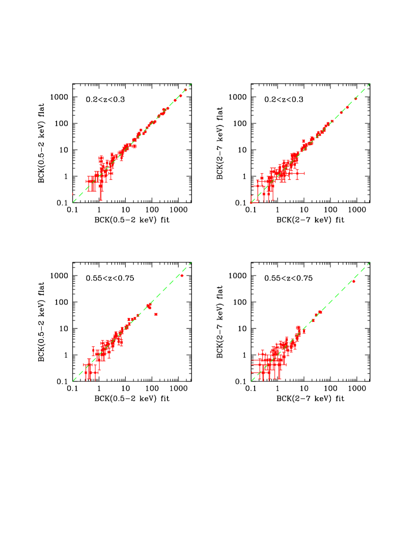
Figure 2: Comparison of the background value (total counts in the 0.5-7 keV band) assuming a flat surface brightness in the inner 3 arcsec ($bck_{flat}$) to the value obtained with a double-beta model fit ($bck_{2bfit}$). The comparison is made for each energy band and each redshift range separately.

In the second step, we further investigate the robustness of our background estimate by fitting the entire surface brightness profile with a single-beta model profile. All the profiles are inspected by eye and fitted with sherpa following the ciao thread. We find that the values $bck_{1bfit}$ obtained with a single-beta model are on average 30% lower than $bck_{flat}$, which may simply indicate that a single beta model is not sufficient to catch the rapid increase of the surface brightness in the center of a cool-core cluster. Therefore, we repeat the fit with a double-beta model. The results are shown in Figure 2 for the soft- and hard- band images, in the low and high redshift bins. We find that on average, there is a good agreement within a few percent. By performing a direct fit of the $bck_{flat}-bck_{2bfit}$ relation, we find that in the low-redshift bin $bck_{2bfit}$ is in average 12% and 8% lower than $bck_{flat}$ in the soft and hard band, respectively, while the slope is consistent with unity within the errors. In the high-redshift bin, we find that $bck_{2bfit}$ is on average 10% lower and 11% higher than $bck_{flat}$, in the soft and hard band, respectively, while the slope is still consistent with unity. We apply this average correction to the background, and verify that the photometry is only marginally affected. However, both methods provide values in good agreement, and at the same time, do not guarantee a control on the actual surface brightness fluctuations in the inner 1.2 arcsec, which still remain an unavoidable uncertainty in this kind of study.

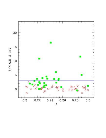
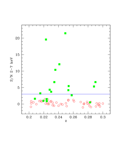
Figure 3: Left panel: S/N in the soft band versus redshift for the low-redshift BCG sample. Green squares show BCGs with unresolved X-ray emission after visual inspection, while empty red circles are nondetections. The horizontal line corresponds to the assumed detection threshold $S/N=3$. Right panel: S/N in the hard band versus redshift for the low-redshift BCG sample. Symbols are the same as in the left panel.

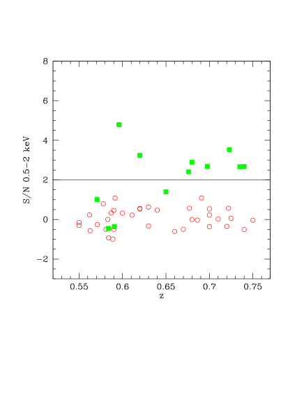
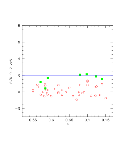
Figure 4: Left panel: S/N in the soft band versus redshift for the high-redshift BCG sample. Green solid circles show BCG with unresolved X-ray emission, while red open denote nondetections. The horizontal line corresponds to the assumed detection threshold $S/N=2$. Note that the brightest source (3C254), with an $S/N\sim 56$, is not shown. Right panel: S/N in the hard band versus redshift for the high-redshift BCG sample. Symbols as in the left panel. Note that the two brightest sources (3C254, at $z=0.74$, and the Phoenix cluster, at $z=0.596$) with an $S/N\sim 38$ and $\sim 59$, respectively, are not shown.

In the two panels of Figure 3 we show the soft- and hard- band S/N for the low-redshift sample plotted against the redshift. Sources with unresolved emission detected by visual inspection at least in one band are shown with green squares, while sources with no apparent unresolved emission in both bands are shown with red circles. We note that the soft-band S/N distribution does not identify a clear threshold to separate sources with and without unresolved emission. When focusing on the low-redshift range, we find that sources with and without unresolved emission cannot be separated on the basis of the S/N for $S/N<3$, while for $S/N>3$ all the sources have been flagged with unresolved emission in our visual inspection. The significant contamination at low $S/N$ is likely due to the presence of complex structures in the cold gas, X-ray coronae, or both. Therefore, we adopt the criterion $S/N>3$ in at least one band to identify sources with reliable unresolved emission among those flagged by visual inspection. This threshold is shown in the panels of Figure 3 as a horizontal line. This criterion identifies 14 BCGs with unresolved nuclear X-ray emission out of 81 ($\sim$ 17%).

For the high-redshift sample, shown in the two panels of Figure 4, the sources with unresolved emission are found at $S/N>2$ in the soft and hard band. Therefore, in this case we adopt a threshold $S/N=2$, lower than in the low-redshift sample. This choice allows us to select 9 sources with visual detection and $S/N>2$ in at least one band. Therefore we have 9 BCGs with unresolved X-ray emission out of 51, corresponding to $\sim$ 18% of the sample, similarly to the low-redshift bin.

In Figure 5 we show the distributions of the 2-7 keV count rate to 2-10 keV energy flux conversion factors for the soft and hard band, used to derive the observed fluxes. The distribution in the soft band is significantly higher than in the hard band, which is due to the effect of the different Galactic absorption columns at the position of the BCG. In addition, another source of variation is due to the mix of exposures taken at different epochs, combined with the progressive degradation of the effective area due to the molecular contamination of the ACIS filters over the years.

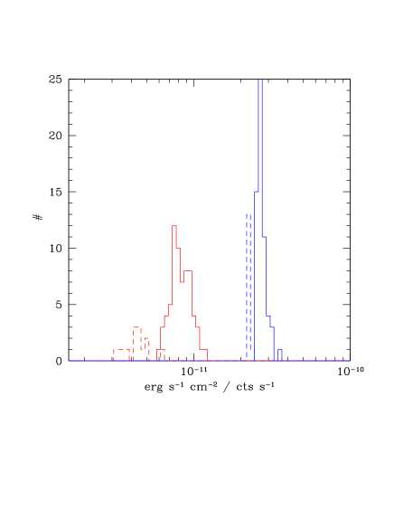
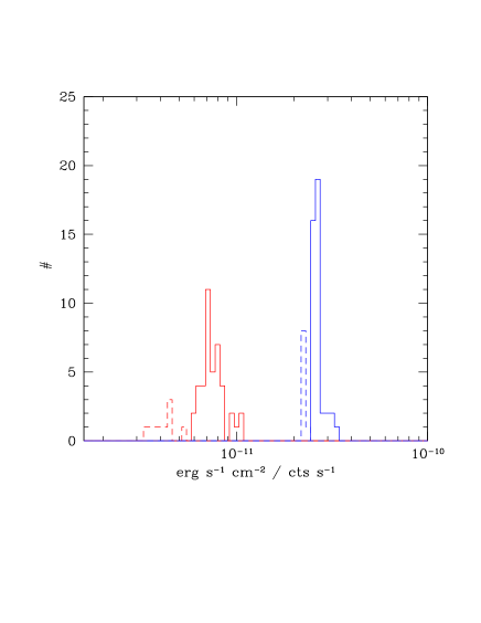
Figure 5: Left panel: the distributions of conversion factors in the soft band and in the hard band (from 2-7 keV to 2-10 keV) are shown with red and blue lines for the low-z sample. The solid lines are for ACIS-I (67 observations), while the dashed lines are for ACIS-S (14 observations). Right panel: same as the left panel for the high-z sample (with 40 observations with ACIS-I and 9 with ACIS-S).

Figure 6: Comparison between hard-band fluxes measured in this work with those measured in Russell et al. (2013) from spectral analysis and Hlavacek-Larrondo et al. (2015) from photometry, shown with black and blue labels, respectively, for the few sources in common. As usual, sources with unresolved emission in the soft or hard band are shown with green filled squares, while sources with upper limits are shown with red empty circles. Upper limits correspond to $3\sigma$ c.l., and all the sources in this plot belong to the low-redshift bin.

In Table 5 and Table 6 we show the photometry of the BCG with unresolved X-ray emission in one or both bands in the $0.2<z<0.3$ and $0.55<z<0.75$ redshift range, respectively. Error bars on photometry include only the (Poissonian) statistical uncertainties, while error bars on energy fluxes also include the uncertainties associated with the ICM surface brightness fluctuations, as previously discussed. Only energy fluxes are increased by 5% and 10% in the soft and hard band, respectively, to account for the flux lost outside the extraction region.

As a check, we compare our photometric hard-band fluxes obtained with conversion factors to the values found in the literature. The comparison for the 7 sources in common with Russell et al. (2013, from spectroscopic analysis) and 5 sources in common with Hlavacek-Larrondo et al. (2015, from photometry) shows a reasonable agreement, considering the different data reduction and the different measurement procedure (see Figure 6). Two sources show statistically significant differences, namely RXC J1459.4-1811 and A2667, for which we measure a hard-band flux about two times lower and about three times higher, respectively, than Russell et al. (2013). We will comment on these two discrepant sources after we present the spectral analysis presented in Section 4.4.

We remark that in Table 5 and Table 6 we report both soft- and hard-band photometry, regardless of the detection band, so that in some cases one of the two fluxes is below the formal threshold ($S/N>3$ and $S/N>2$ in the low- and high-z sample, respectively). In the next section, we focus only on the sources with a firm detection in the hard band, therefore above the selection threshold. This reduces the number of sources to 12 and 5 in the low- and high-z sample, respectively.

Table 5: Soft- and Hard- Band Photometry of BCGs in the $0.2<z<0.3$ Redshift Range with Unresolved Emission Visually Detected and $S/N>3$ in at Least One Band. Conversion factors are given in units of $10^{-12}$ and $10^{-11}$ erg s^-1 cm^-2 / cts s^-1 in the soft and hard band, respectively. Soft and hard energy flux values are given in units of $10^{-15}$ erg s^-1 cm^-2. Error bars on counts include only the statistical uncertainties, while errors on the energy flux and hard-band luminosity include also the uncertainties associated to the ICM surface brightness fluctuations. Hard-band luminosity is computed after equation 1. Fluxes and luminosities are corrected for Galactic absorption but not for intrinsic absorption.

Cluster	Soft Net Counts	Hard Net Counts	Soft S/N	Hard S/N	Soft CF	Hard CF	Soft Flux	Hard Flux	$log(LX_{hard})$
RXC J1504-0248	$212.75\pm 71.61$	$156.27\pm 48.10$	2.97	3.24	9.186	2.601	$13.9\pm 5.4$	$30.18\pm 10.50$	$42.59\pm 0.13$
G256.55-65.69	$33.20\pm 8.90$	$4.81\pm 4.68$	3.69	1.01	8.957	2.688	$10.9\pm 3.4$	$4.96\pm 5.46$	$41.82\pm 0.32$
PKS 1353-341	$199.25\pm 18.30$	$534.03\pm 27.17$	10.83	19.59	1.083	2.860	$74.9\pm 8.0$	$555.29\pm 31.92$	$43.89\pm 0.02$
A2390	$130.96\pm 33.16$	$79.25\pm 18.11$	3.94	4.35	4.318	2.227	$6.4\pm 1.9$	$20.90\pm 5.39$	$42.48\pm 0.10$
A2667	$8.87\pm 12.12$	$30.19\pm 7.98$	0.73	3.74	3.447	2.188	$3.3\pm 5.3$	$75.33\pm 22.49$	$43.05\pm 0.11$
A2146	$133.67\pm 29.72$	$138.44\pm 20.70$	4.48	6.66	7.724	2.584	$2.9\pm 0.7$	$10.48\pm 1.77$	$42.21\pm 0.07$
RXC J1459.4-1811	$76.23\pm 20.28$	$192.31\pm 18.42$	3.74	10.38	4.900	2.235	$9.9\pm 3.1$	$119.29\pm 12.91$	$43.27\pm 0.04$
4C+55.16	$702.57\pm 42.52$	$274.64\pm 22.64$	16.49	12.08	4.140	2.210	$34.0\pm 2.4$	$74.31\pm 6.92$	$43.09\pm 0.04$
A2125	$25.09\pm 6.85$	$-0.28\pm 1.71$	3.61	-0.16	6.484	2.594	$2.0\pm 0.6$	$-0.09\pm 0.64$	-
CL 2089	$175.79\pm 28.98$	$672.77\pm 31.22$	6.04	21.48	4.408	2.243	$20.0\pm 3.8$	$408.38\pm 21.41$	$43.86\pm 0.02$
RXC J1023.8-2715	$80.95\pm 24.36$	$62.81\pm 14.78$	3.31	4.22	4.605	2.234	$10.8\pm 3.8$	$42.44\pm 11.29$	$42.89\pm 0.10$
CL 0348	$102.68\pm 27.63$	$80.84\pm 14.70$	3.70	5.46	4.401	2.224	$9.7\pm 3.0$	$40.58\pm 8.34$	$42.87\pm 0.08$
A611	$236.73\pm 20.40$	$53.27\pm 9.90$	11.55	5.33	3.809	2.200	$26.5\pm 2.6$	$36.09\pm 7.58$	$42.95\pm 0.08$
3C438	$102.87\pm 20.06$	$106.92\pm 15.94$	5.10	6.66	6.265	2.311	$4.3\pm 1.0$	$17.17\pm 2.89$	$42.63\pm 0.07$

Table 6: Soft- and Hard Band Photometry of BCGs with Unresolved Emission Detected with $S/N>2$ in at Least One Band, in the $0.55<z<0.75$ Redshift Range. Conversion factors are given in units of $10^{-12}$ and $10^{-11}$ erg s^-1 cm^-2 / cts s^-1 in the soft and hard band, respectively. Soft and hard energy flux values are given in units of $10^{-15}$ erg s^-1 cm^-2. Error bars on counts include only the statistical uncertainties, while errors on the energy flux and hard-band luminosity include also the uncertainties associated to the ICM surface brightness fluctuations. Hard-band luminosity is computed after equation 1. Fluxes and luminosities are corrected for Galactic absorption but not for intrinsic absorption.

Cluster	Soft Net Counts	Hard Net Counts	Soft S/N	Hard S/N	Soft CF	Hard CF	Soft Flux	Hard Flux	$log(LX_{hard})$
SPT-CL J2344-4243	$263.33\pm 54.86$	$4638.24\pm 84.55$	4.79	54.79	1.006	2.996	$21.6\pm 5.2$	$1184.35\pm 24.40$	$45.19\pm 0.01$
RCS 1419+5326	$33.60\pm 10.27$	$3.31\pm 3.95$	3.24	0.82	3.886	2.219	$2.4\pm 0.9$	$1.43\pm 1.94$	$42.31\pm 0.37$
ACT J0206-0114	$9.93\pm 4.03$	$-0.21\pm 0.51$	2.41	-0.35	8.207	2.527	$2.9\pm 1.4$	$-0.20\pm 0.54$	-
SDSS J1004+4112	$33.57\pm 11.51$	$12.68\pm 6.01$	2.89	2.08	4.566	2.217	$0.7\pm 0.3$	$1.27\pm 0.68$	$42.36\pm 0.19$
MACS 0744.8+3927	$42.39\pm 15.72$	$22.00\pm 10.29$	2.68	2.12	7.160	2.581	$3.6\pm 1.5$	$7.03\pm 3.72$	$43.13\pm 0.18$
SPT-CL J2043-5035	$55.28\pm 15.59$	$15.73\pm 8.33$	3.52	1.87	7.918	2.611	$5.8\pm 1.9$	$5.72\pm 3.42$	$43.07\pm 0.20$
RCS 1107.3-0523	$19.04\pm 7.05$	$-0.71\pm 1.83$	2.66	-0.37	4.259	2.253	$0.9\pm 0.4$	$-0.19\pm 0.55$	-
3C254	$3224.95\pm 66.61$	$1502.19\pm 43.30$	48.34	34.61	3.369	2.176	$386.2\pm 9.3$	$1217.29\pm 39.65$	$45.42\pm 0.01$
SPT-CL 0001-5748	$25.52\pm 9.46$	$8.53\pm 5.38$	2.67	1.56	7.383	2.613	$6.6\pm 2.8$	$8.14\pm 5.79$	$43.25\pm 0.23$

4.2 The Fraction of X-Ray Luminous BCG as a Function of $L_{X}$

The fraction of X-ray emitting BCGs above a given X-ray luminosity is computed as

$$F_{BCG}(>L_{X})=\Sigma_{>L_{X}}{1\over{N(L_{up}<L_{X})}}$$ (2)

where the sum is computed for all the BCGs with a hard band X-ray luminosity higher than $L_{X}$, and $N(L_{up}<L_{X})$ is the number of clusters for which the luminosity corresponding to the detection threshold is lower than $L_{X}$, in other words, all the clusters where we should have seen the AGN in the BCG if above $L_{X}$. Given our selection threshold $S/N>3$ and $S/N>2$ in the hard band for the low- and high-z sample, respectively, we have a well-defined detection threshold in hard-band luminosity at each BCG position. This value defines the completeness of our sample in luminosity. Clearly, the completeness correction mostly affects the lowest luminosity bins, and the correction is more important at higher redshift.

The cumulative fractions of X-ray luminous BCGs as a function of $L_{X}$ in the low- and high-redshift bins are shown in Figure 7. Error bars are the Poissonian error bars due to the finite numbers, so that roughly $\sigma=\sqrt{(N(L_{BCG}>L_{X})}/N(L_{up}<L_{X})$, where $N(L_{BCG}>L_{X})$ is the number of BCGs with a hard-band luminosity higher than $L_{X}$. In both samples, the lowest luminosity detected is $\geq 10^{42}$ erg s^-1. The average slope of the cumulative fraction in the low-z bin is between $\sim-0.6$ and $\sim-1$, with a very weak hint of a steeper slope at $L_{X}\geq 10^{43}$ erg s^-1. The limited statistics in the high-redshift bin, where we have only five sources, prevents us from drawing any conclusion on the slope. However, we are able to establish that the normalization of the X-ray luminosity function in the Seyfert-like luminosity range ($L_{X}<10^{44}$ erg s^-1) is consistent with the low-z sample, while a striking difference is given by the presence of two extremely luminous quasars (in the BCG of the Phoenix cluster and 3C254) that are completely absent at low redshift. Taken at face value, the measured fraction of X-ray luminous BCGs in our sample points toward no evolution below $10^{44}$ erg s^-1 and a possible evolution above this value. This result is in broad agreement with Hlavacek-Larrondo et al. (2013b), where they find significant positive evolution with redshift. However, their results were based on a sample of X-ray bright clusters with strong cavities, while we aim at including the widest range of halo masses and environment offered by the Chandra archive. Clearly, any conclusion on evolution must await the use of the entire Chandra archive, with the same strategy as was used in this work. Eventually, on the basis of a larger statistics, we will explore the X-ray luminosity function of BCGs in subsamples extracted from complete and well-defined cluster catalogs.

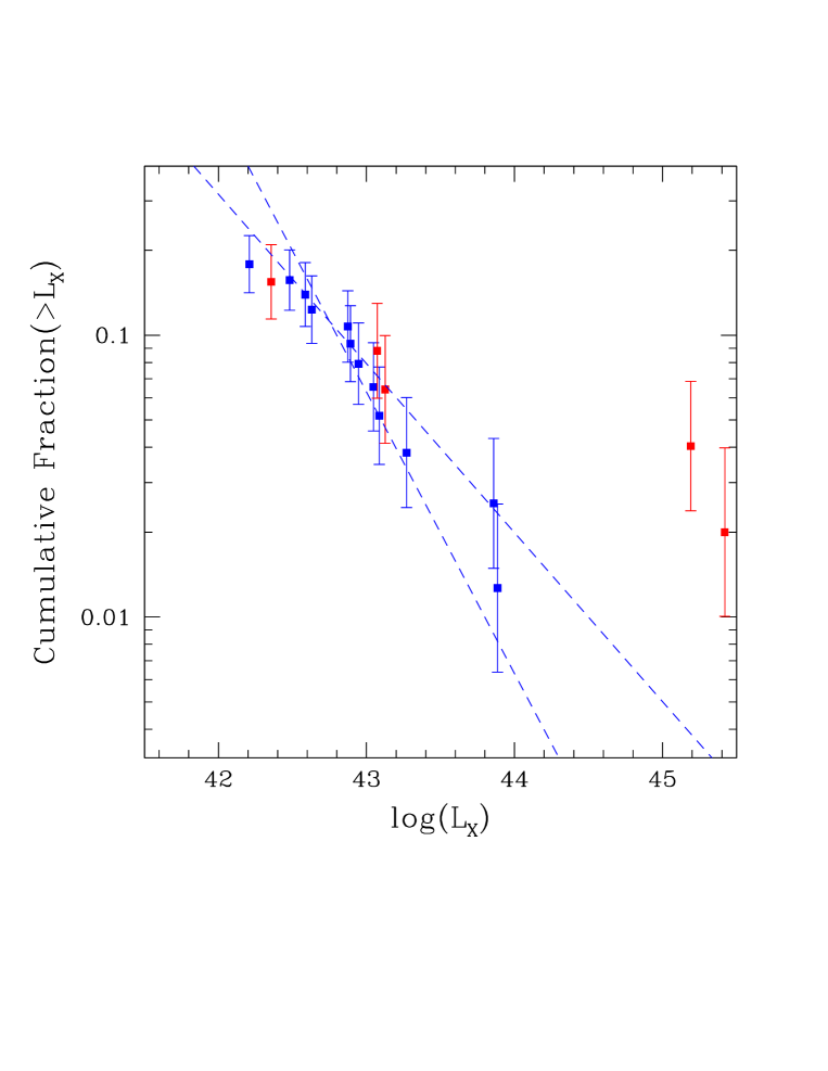
Figure 7: Cumulative fraction of X-ray luminous BCGs as a function of the hard-band $L_{X}$ in the redshift range $0.2<z<0.3$ (blue squares) and $0.55<z<0.75$ (red squares). The two dashed lines bracketing the cumulative luminosity distribution in the low-redshift bin, have slopes of $-0.6$ and $-1$.

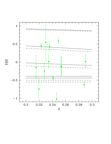
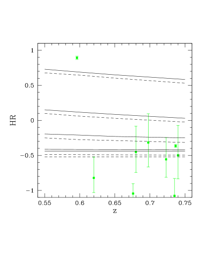
Figure 8: Left panel: hardness ratio for the sources with unresolved X-ray emission in the soft or hard band, in the redshift range $0.2<z<0.3$. Erorr bars correspond to 1$\sigma$ confidence level. Solid (dashed) lines correspond to typical hardness ratios measured with ACIS-I (ACIS-S) for an intrinsic equivalent hydrogen-absorbing column of (from bottom to top) $10^{20}$, $10^{21}$, $10^{22}$, $3\times 10^{22}$, and $10^{23}$ cm^-2. Right panel: same as in the left panel for the sources in the $0.55<z<0.75$ redshift range.

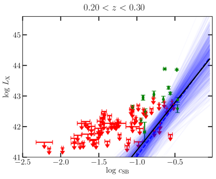
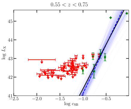
Figure 9: Left panel: hard-band luminosity versus the BCG concentration parameter in the $0.2<z<0.3$ redshfit range. Sources with positive photometry in the hard band and $S/N>3$ in at least one band are shown with green solid squares. Red arrows shows the $3\sigma$ upper limits for the BCGs with no nuclear emission. Error bars correspond to the 1$\sigma$ confidence level. Black solid and blue dashed lines are the best fit obtained from a censored-data analysis using the software ASURV and LINMIX_ERR, respectively. The light blue lines represent 400 different realizations of the $\log L_{\rm X}-\log c_{SB}$ relation from LINMIX_ERR. Right panel: same as in the left panel for the sources with positive photometry in the hard band and $S/N>2$ in the $0.55<z<0.75$ redshift range.

4.3 Average Spectral Properties and Connection with Cool Cores

For a first-cut evaluation of the spectral properties of the X-ray emitting BCGs, we compute their hardness ratio, simply defined as $HR\equiv(C_{hard}-C_{soft})/(C_{hard}+C_{soft})$, where $C_{hard}$ and $C_{soft}$ are the source net counts measured in the hard and soft band, respectively, and corrected for vignetting. In Figure 8, left panel, we show the hardness ratios for the sources with unresolved X-ray emission in at least one of the two bands in the low-redshift bin. We also plot solid (dashed) lines corresponding to the typical hardness ratio measured with ACIS-I (ACIS-S) for an intrinsic equivalent hydrogen-absorbing column of (from bottom to top) $10^{20}$, $10^{21}$, $10^{22}$, $3\times 10^{22}$, and $10^{23}$ cm^-2. These representative curves are computed for a typical Chandra observation at the aimpoint for a spectrum with an intrinsic emission described by a power law of $\Gamma=1.8$, considering an average Galactic absorbing column of $3\times 10^{20}$ cm^-2. We note that roughly half of the sample in the low-redshift bin shows hints of intrinsic absorption ($HR\geq 0$, corresponding roughly to $10^{22}$ cm^-2) in the soft band. This implies that to compute the total intrinsic X-ray luminosity, we need to correct for intrinsic absorption below 2 keV. In Figure 8, right panel, we show the hardness ratio for the sources with unresolved X-ray emission in at least one of the two bands in the high-redshift sample. Only one source is clearly absorbed (SPT-CL J2344-4243, see, e.g. Tozzi et al., 2015), while the other sources are consistent with the spectrum of unabsorbed AGN ($HR\sim-0.5$).

We also compute the concentration parameter (defined as the ratio of the energy flux in the soft band within 40 kpc to that within 400 kpc) at the BCG position for all our groups and clusters. The two fluxes are obtained after removing unresolved emission, including the central AGN when present. Our definition of the concentration parameter is different from that of Santos et al. (2008), which is computed at the peak of the X-ray surface brightness. Clearly, the two definitions agree only when the BCG is located precisely at the maximum of the diffuse X-ray emission. In Figure 9 we show the measured hard band luminosity for the sources with positive hard band photometry detected at least in one band in the low and high redshift bins. We find that, on one hand, BCGs with nuclear emission are preferentially in stronger cores, with concentration parameter $c_{SB}>0.1$. On the other hand, only one-third of the clusters with $c_{SB}>0.1$ host an AGN with $L_{X}>10^{42}$ erg s^-1 in the BCG. For example, we do not find nuclear activity in MS 0735.6+7421, which hosts a strong cool core and is one of the most powerful mechanical outburst known to date (McNamara et al., 2005; Gitti et al., 2007), as already shown in Figure 1. One may argue that some level of nuclear X-ray emission may be present in all the strong cool cores, possibly hidden by the overwhelming ICM emission. To explore this possibility and the effects of the many upper limits, we perform a censored-data analysis on the $log(L_{X})$-$log(c_{SB})$ relation. Owing to the large number of upper limits, we are aware that we are dealing with an extreme situation, and the results should be critically assessed before drawing any conclusion. We adopt the LINMIX_ERR software (Kelly, 2007). This method accounts for measurement errors on both independent and dependent variable, nondetections, and intrinsic scatter by adopting a Bayesian approach to compute the posterior probability distribution of parameters, given observed data. This has been argued to be among the most robust regression algorithms with the possibility of reliable estimation of intrinsic random scatter on the regression. We also consider the Astronomy Survival Analysis software package (ASURV rev. 1.2; Isobe et al. 1990; Lavalley et al. 1992), which is widely used in the literature. ASURV implements the bivariate data-analysis methods and also properly treats censored data using the survival analysis methods (Feigelson & Nelson 1985; Isobe et al. 1986). We have employed the full parametric estimate and maximized regression algorithm to perform the linear regression of the data. The results are shown in Figure 9 with a continuous and dashed line, from the ASURV and LINMIX_ERR analysis, respectively. For the low-redshift sample, we find a slope $\sim 3$, while in the high-redshift sample the slope is even steeper $\geq 4$. Moreover, at low redshift, we find a low normalization, driven by the many upper limits at $c_{SB}>0.1$, while at high redshift the normalization is driven by the detections, given the very low number of upper limits at $c_{SB}>0.1$. The main conclusion we can reach from our analysis is that AGN with $L_{X}>10^{42}$ erg s^-1 ($L_{X}>10^{43}$ erg s^-1) appear only above $c_{SB}>0.1$ in the low-(high-) redshift range. In addition, above the same X-ray luminosity threshold, AGN do not sit in non-cool-core cluster ($c_{SB}<0.11$).

As we have discussed, spectral analysis may be helpful in identifying nonthermal emission, possibly associated with a central AGN, through the measurement of spectra harder than expected from the thermal ICM, as has been proposed in Hlavacek-Larrondo et al. (2013b). However, as explained in Section 3.2, this type of diagnostic based on spectral shape needs a very high S/N, and therefore is not suitable for exploring the low-luminosity range. Therefore, we limit our spectral analysis to the sources with unresolved emission detected with our photometry, as described in the next section.

4.4 X-Ray Spectral Analysis

We perform a standard spectral analysis on the sources listed in Table 5 and 6 using a simple physical model consisting in an absorbed power law plus a local Galactic absorption (Xspec model tbabs $\times$ zwabs $\times$ pow). We extract source and background spectra from the same extraction regions as we used for photometry. Calibration files are the same used to compute the conversion factors. Our spectral analysis is therefore based on the same background subtraction used in our photometry. Our aim is to confirm our results and explore the distribution of intrinsic absorption. However, we remark that spectral analysis in these extreme conditions of strong background can have a complex effect on the best-fit values of the spectral parameters. A proper approach would require the combined analysis of an absorbed power law plus a thermal component at the same time. Clearly, this is feasible only for very bright sources because of the strong degeneracy of a composite model. The spectral analysis discussed in this work should therefore be simply regarded as an extension of our photometric study.

4.4.1 Spectral Analysis of Sources at $0.2<z<0.3$

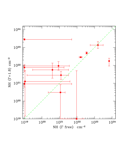
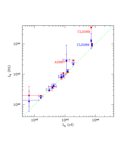
Figure 10: Left panel: comparison of best-fit values for intrinsic absorption $N_{H}$ obtained with a free spectral slope, and with a slope frozen to $\Gamma=1.8$ for the sources in the low-redshift sample. Right panel: rest-frame 2-10 keV, unabsorbed luminosity obtained from spectral analysis, compared to the value obtained from aperture photometry, and not corrected for intrinsic absorption. Values obtained with a free spectral slope are shown in blue, while those obtained for $\Gamma=1.8$ are shown in red.

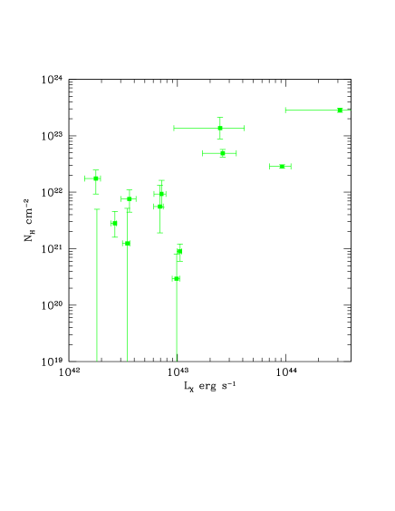
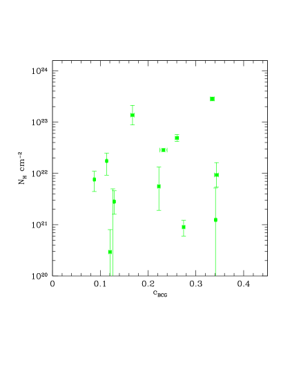
Figure 11: Left: intrinsic absorption $N_{H}$ compared to the rest-frame 2-10 keV, unabsorbed luminosity as obtained from spectral analysis for the sources in the low-redshift sample. Right: intrinsic absorption obtained from spectral fits compared to the concentration parameter at the BCG position.

In the low-redshift bin, we force the spectral analysis on all our sources, including those with low S/N, except for A2125, which is the source detected with the lowest number of net counts. The best-fit values of the intrinsic spectral slope, intrinsic absorption, and unabsorbed hard-band rest-frame luminosity are shown in Table 7. As a simple consistency test, we check that the soft and hard flux values obtained with our spectral analysis are consistent with those obtained with simple aperture photometry within the errors, finding a good agreement. We find that in general, best-fit values for $\Gamma$ range from 1 to 2 with a typical errorbar of 0.25. In some cases, we find anomalously large or low spectral slope (G256.55-65.69, A2146, and CL 2089), showing that for a significant part of our sample, the best-fit values may be driven by spurious residuals that are due to the direct background subtraction. We notice that typical values of $\Gamma$ for AGN in the Seyfert range of luminosities, are $1.6<\Gamma<2.0$, while our best fit $\Gamma$ are lower on average. Since we are performing spectral analysis in extreme conditions, and small background fluctuations may affect the entire energy range, we also perform the spectral analysis by freezing the slope of the power law to $\Gamma=1.8$, which clearly has a significant effect on the best fit values of the intrinsic absorption. In Figure 10, left panel, we compare the values of the intrinsic absorption obtained with free power law and with power law frozen to $\Gamma=1.8$. The largest differences are obtained for the sources with extremely large or extremely low $\Gamma$, as expected because of the strong degeneracy between $N_{H}$ and $\Gamma$.

In Figure 10, right panel, we investigate whether the unabsorbed luminosities obtained with the spectral analysis are consistent with those obtained directly from aperture photometry and our average conversion factors. We find a good agreement, finding that, as expected, the intrinsic absorption of our sources has a modest impact on the luminosity. Focusing on the two sources with $L_{X}$ discrepant from the values reported in Russell et al. (2013), we find that the hard luminosity of RXC J1459 is 1.5 times higher from spectral analysis, which agree with the value found in Russell et al. (2013). However, the hard luminosity from the spectral analysis for A2667 increases, despite the large error bars, and this increases the discrepance with respect to Russell et al. (2013). Such a difference could be explained only with a background three times larger than estimated, which is not acceptable. We note, however, that the hard X-ray emission is displaced more than 2 arcsec from the peak of the soft emission, and the hard flux may be severely underestimated if the BCG position is not firmly secured by the optical image.

We finally note that all the spectral fits have an acceptable C-statistics, except for two fits. In the cases of A2146 and CL 2089, we obtain a high C-statistics value, and the visual inspection of the residuals shows that this is due to bumps in the low-energy range and at the position of the iron emission line complex. This strongly suggests that a significant contribution from the ICM thermal emission has not been properly removed by our direct background subtraction. We also note that these residuals cannot be eliminated by tuning the backscale parameter, showing that the problem is not due to a trivial issue of background scaling, but it is related to significant variation of the thermal properties in the inner 10 kpc. This aspect can be treated only with a multi-component spectral model, an approach that goes beyond the scope of this work.

In Figure 11 we present preliminary results related to the distribution of intrinsic absorption. In the left panel, we show the relation between $N_{H}$ and $L_{X}$. We note that the lack of unabsorbed bright ($L_{X}>10^{43}$ erg s^-1) AGN is significant, while the lack of strongly absorbed, lower luminosity AGN may be due to selection effects against faint sources. The statistics is in any case too low to draw any conclusion. In the right panel of Figure 11 we show the relation between $N_{H}$ and the ICM concentration parameter, which does not show any obvious trend.

Table 7: Spectral Analysis of the Sources in the Low-redshift Bin. The best-fit parameters are obtained with the model tbabs ( zwabs $\times$ pow) with $\Gamma$ free and with $\Gamma=1.8$. $L_{X}$ corresponds to the unabsorbed, rest-frame 2-10 keV luminosity. Error bars and upper limits corresponds to $1\sigma$ confidence level.

Cluster	$\Gamma$	$N_{H}/10^{22}$ cm-2	$log(L_{X}$)
RXC J1504-0248	$1.59_{-0.22}^{+0.35}$	$<0.40$	$42.56_{-0.05}^{+0.03}$
G256.55-65.69	$3.28_{-0.95}^{+1.55}$	$0.94_{-0.80}^{+1.52}$	$42.11_{-0.37}^{+0.30}$
PKS 1353-341	$1.17_{-0.14}^{+0.15}$	$1.63_{-0.31}^{+0.33}$	$43.95_{-0.08}^{+-0.03}$
A2390	$1.48_{-0.27}^{+0.29}$	$0.12_{-0.12}^{+0.21}$	$42.47_{-0.05}^{+0.03}$
A2667	$2.14_{-0.87}^{+2.17}$	$15.6_{-9.9}^{+15.6}$	$43.45_{-0.4}^{+0.47}$
A2146	$4.48_{-0.16}^{+0.22}$	$67.7_{-0.06}^{+0.07}$	$42.23_{-0.05}^{+0.03}$
RXC J1459.4-1811	$1.36_{-0.13}^{+0.23}$	$3.49_{-0.1}^{+0.56}$	$43.33_{-0.05}^{+0.03}$
4C+55.16	$1.49_{-0.06}^{+0.06}$	$<0.5$	$43.10_{-0.03}^{+0.013}$
CL 2089	$-0.78_{-0.09}^{+0.08}$	$<0.5$	$44.10_{-0.3}^{+0.2}$
RXC J1023.8-2715	$1.13_{-0.23}^{+0.31}$	$0.04_{-0.03}^{+0.29}$	$42.91_{-0.06}^{+0.04}$
CL 0348	$1.03_{-0.24}^{+0.28}$	$0.09_{-0.08}^{+0.28}$	$42.91_{-0.07}^{+0.04}$
A611	$2.03_{-0.21}^{+0.22}$	$0.11_{-0.09}^{+0.10}$	$42.94_{-0.07}^{+0.05}$
3C438	$1.00_{-0.16}^{+0.21}$	$<0.18$	$42.63_{-0.07}^{+0.03}$
RXC J1504-0248	$1.80$	$0.12_{-0.12}^{+0.39}$	$42.54_{-0.05}^{+0.02}$
G256.55-65.69	$1.80$	$<0.5$	$42.26_{-0.37}^{+0.30}$
PKS 1353-341	$1.80$	$2.86_{-0.19}^{+0.20}$	$43.96_{-0.12}^{+0.08}$
A2390	$1.80$	$0.28_{-0.12}^{+0.18}$	$42.42_{-0.04}^{+0.02}$
A2667	$1.80$	$13.7_{-4.9}^{+7.6}$	$43.39_{-0.43}^{+0.22}$
A2146	$1.80$	$1.75_{-0.82}^{+0.72}$	$42.25_{-0.10}^{+0.04}$
RXC J1459.4-1811	$1.80$	$4.89_{-0.68}^{+0.85}$	$43.42_{-0.19}^{+0.12}$
4C+55.16	$1.80$	$0.09_{-0.03}^{+0.03}$	$43.02_{-0.03}^{+0.01}$
CL 2089	$1.80$	$28.3_{-2.3}^{+2.5}$	$44.50_{-0.50}^{+0.47}$
RXC J1023.8-2715	$1.80$	$0.56_{-0.37}^{+0.78}$	$42.84_{-0.06}^{+0.03}$
CL 0348	$1.80$	$0.93_{-0.39}^{+0.69}$	$42.85_{-0.07}^{+0.04}$
A611	$1.80$	$0.03_{-0.03}^{+0.05}$	$42.99_{-0.04}^{+0.03}$
3C438	$1.80$	$0.76_{-0.31}^{+0.34}$	$42.56_{-0.08}^{+0.06}$

4.4.2 Spectral Analysis of Sources at $0.55<z<0.75$

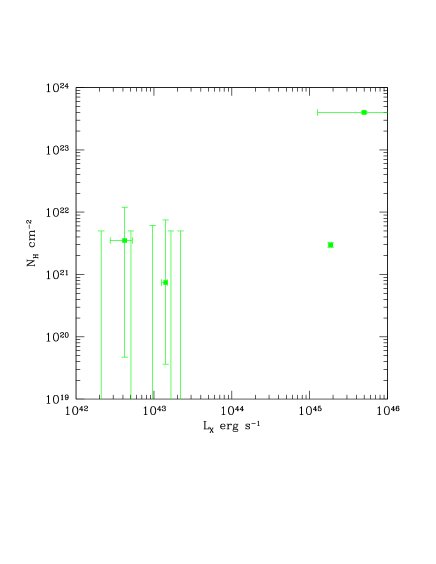
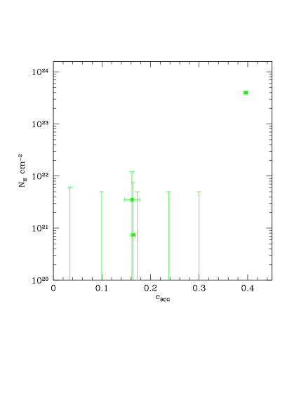
Figure 12: Left: rest-frame 2-10 keV, unabsorbed luminosity obtained from spectral analysis for the sources in the high-redshift sample, compared to the intrinsic absorption. Right: intrinsic absorption obtained from the spectral fit compared to the concentration parameter at the BCG position.

In the high-redshift bin, we can perform the fit with the spectral slope $\Gamma$ free only for two sources, finding again rather flat slopes ($\Gamma\sim 1.2-1.3$). For all the other sources except for ACT J0206 and RCS 1107 (which have fewer than 20 total net counts), we are able to obtain a meaningful spectral fit with spectral slope frozen to $\Gamma=1.8$. The results are reported in Table LABEL:fit_z0.55_0.75. Clearly, the results on $N_{H}$ are limited with respect to the low-redshift bin, since the energy range most sensible to absorption is shifted out of the observed range. We are able to confirm that only one source (SPT-CL J2344) has significant absorption, while all the other sources are consistent with being unabsorbed. In Figure 12, we show the relation between $N_{H}$ and $L_{X}$ (left panel) and between $N_{H}$ and $c_{SB}$, which are clearly dominated by upper limits.

Table 8: Spectral Analysis of the Sources in the High-redshift Bin. The best-fit parameters are obtained with the model tbabs ( zwabs $\times$ pow) with $\Gamma$ free and with $\Gamma=1.8$. $L_{X}$ corresponds to the unabsorbed, rest-frame 2-10 keV luminosity. Error bars and upper limits corresponds to $1\sigma$ confidence level.

Cluster	$\Gamma$	$N_{H}/10^{22}$ cm-2	$log(L_{X}$)
SPT-CL J2344-4243	$1.16_{-0.10}^{+0.10}$	$27.2_{-2.0}^{+2.2}$	$45.49_{-0.39}^{+0.38}$
3C254	$1.32_{-0.02}^{+0.02}$	$<0.04$	$45.33_{-0.01}^{+0.01}$
SPT-CL J2344-4243	$1.80$	$39.8_{-1.3}^{+1.4}$	$45.70_{-0.60}^{+0.59}$
RCS 1419+5326	$1.80$	$<0.5$	$42.70_{-0.2}^{+0.15}$
SDSS J1004+4112	$1.80$	$<0.5$	$42.32_{-0.15}^{+0.08}$
MACS 0744.8+3927	$1.80$	$0.07_{-0.06}^{+0.68}$	$43.15_{-0.05}^{+0.02}$
SPT-CL J2043-5035	$1.80$	$<0.5$	$43.22_{-0.4}^{+0.4}$
3C254	$1.80$	$0.30_{-0.02}^{+0.02}$	$45.27_{-0.02}^{+0.01}$
SPT-CL 0001-5748	$1.80$	$<0.5$	$43.34_{-0.4}^{+0.4}$

We conclude that our spectral analysis confirms the results on luminosity and average spectral properties obtained with simple aperture photometry, showing that our approach is effective in studying the X-ray properties of AGN in BCGs. We also obtain a preliminary investigation of the distribution of intrinsic absorption, which is necessarily limited by the statistical error and the small number of sources.

4.5 Comparison of X-ray and Radio Properties

Figure 13: Left panel: Radio (1.4  GHz) and hard X-ray flux scatter plot for BCGs with unresolved emission (green solid squares and black triangles) and without unresolved emission (red empty circles) in the redshift range $0.2<z<0.3$. Radio flux is the integrated 1.4 GHz flux from NVSS and FIRST, shown as squares and triangles, respectively. Right panel: the same as in the left panel, where the radio flux is measured at 5.0 GHz by Hogan et al. (2015).

Figure 14: Results from the ASURV regression (solid black line) and the LINMIX_ERR (dashed blue line) on the correlation between hard X-ray flux and radio flux density at 1.4  GHz above 3 mJy. Light blue lines represent 200 different realizations of the relation from LINMIX_ERR.

We also explore the relation between radio and hard X-ray flux in our BCGs. We identify radio counterparts of our BCGs in the NRAO VLA Sky Survey (NVSS,, Condon et al., 1998) and Faint Images of the Radio Sky at Twenty-cm (FIRST, Helfand et al., 2015). NVSS is complete above $\sim 2.5\,$mJy at 1.4 GHz for $decl.>-40^{\circ}$, while the FIRST catalog released in 2014 December covers about 10,575 square degrees of sky both in the northern and southern hemispheres, with the detection threshold of $\sim 1$ mJy at 1.4 GHz. We adopt a simple matching criterion, selecting the NVSS and FIRST sources listed in the corresponding catalogs that are closest to the X-ray position of the BCG within a radius of 20 arcsec and 2 arcsec for NVSS and FIRST, respectively. A large matching radius is recommended also for very bright sources in NVSS, where 40% of the FWHM beam size is 20 arcsec, and the FWHM is 45 arcsec. Since the FIRST resolution is 5.4 arcsec FWHM on average, a matching radius of 2 arcsec is chosen for consistency with the 20 arcsec radius used for NVSS sources. In the low-redshift bin, we identify 29 radio counterparts of our BCGs in NVSS out of 65 sources covered by the survey. Of the 65 sources with NVSS data, 13 also have unresolved X-ray emission in the hard band. For all the other sources with NVSS coverage, we assume a conservative upper limit of 2.5 mJy. We also identify 14 radio counterparts of BCGs out of 29 fields covered by FIRST.

In Figure 13, left panel, we show the X-ray detected BCGs with green squares, while all the other radio counterparts, with only an X-ray flux upper limit, are shown with red circles. We note that X-ray emission appears at any radio power, with a slight preference for low power. In any case, there are no hints of a correlation between hard X-ray and radio emission from BCGs in the $0.2<z<0.3$ redshift range. In the right panel of Figure 13 we also show the scatter plot of the X-ray and 5 GHz radio flux for the 22 sources in common with the sample studied by Hogan et al. (2015). A visual inspection of Figure 13 shows that there are no clear signs of a correlation between the hard flux $F_{H}$ and the radio flux density $F_{R}$ both at 1.4 GHz and 5 GHz (left and right panel, respectively). A censored-data analysis is very challenging because of the many double upper limits. If we search for a correlation for radio flux densities above $\sim 3$ mJy at 1.4 GHz (just above the completeness level of the NVSS), we are able to obtain a best fit with LINMIX_ERR and ASURV. In both cases we find a slope consistent with zero and therefore no signs of correlation (see Figure 14). Russell et al. 2013 (see their section 3.6) did not find a correlation between the nuclear radio 5 GHz and X-ray fluxes either. The absence of a radio correlation suggests that massive sub-relativistic outflows may be the primary driver of kinetic feedback, instead of relativistic jets.

Finally, we note a few cases where a radio source is present in the NVSS field of view close to the BCG, but is not listed in the NVSS catalog, and therefore is not included in our preliminary cross correlation between our BCG and radio counterpart. We stress that a high-resolution follow-up of our BCG with JVLA is needed to firmly identify counterparts of our BCG and to exclude interlopers or non-BCG cluster members, as shown in a few cases in our program of JVLA observation of BCG in the CLASH sample (Yu et al., 2018).

5 Discussion: Implications for AGN Feeding and Feedback

Keeping in mind the limited statistics, we discuss here some implications for the accretion and feedback mode tied to the SMBHs at the center of BCGs and the associated phenomenology in the X-ray and radio bands. As introduced in §1, the maintenance mode of AGN feedback occurs via mechanical injection of energy (McNamara & Nulsen 2012 for a review). Ultrafast AGN outflows and/or relativistic jets are launched within the inner 100 gravitational radii from the SMBH, as shown by high-quality X-ray data (e.g. Nardini et al., 2015) and confirmed by general-relativistic magnetohydrodynamics (MHD) simulations (see Sa̧dowski & Gaspari 2017 and references within). Such simulations imply that below a few percent of the Eddington rate, the radiative power is expected to be fewer than the kinetic input (see also Russell et al. 2013). Consistently with this picture, we find that less than 20% of BCGs are X-ray bright with a cutoff near $10^{43}$ erg s^-1 in the low-z bin. Therefore, only a handful of sources appear to approach the radiatively efficient regime. We thus expect mechanical feedback to dominate over radiative feedback (radiation pressure or Compton heating) also in our sample. Note that the total power AGN outburst in clusters can reach $\sim 10^{45}$ erg s^-1, as observed (Hlavacek-Larrondo et al., 2015) and predicted by simulations (e.g., Gaspari et al. 2012), thereby our nuclear X-ray luminosities may be 100 - 1000 times lower than the maximal injected AGN power. In this framework, the investigation of the nuclear luminosity of BCG at higher redshift may be key to constrain the switching of the feedback mode from mechanical to radiatively efficient, as has been suggested by Hlavacek-Larrondo et al. (2013a) for clusters with clear cavities in the ICM. Radiative feedback is indeed expected to increase at higher redshift due to the halos are progressively smaller and SMBH masses are progressively smaller, and hence Eddington ratios are larger.

Our approach may provide further constraints to the feedback mechanism. For example, the absence of evolution in the bulk of the population at moderate luminosities ($L_{X}<10^{44}$ erg s^-1), if found in a larger sample of virialized halos with no obvious selection bias and on a wider redshift range extending beyond $z=1$, would imply that mechanical AGN feedback is tightly self-regulated since at least $\sim$ 7 Gyr, regardless of the dynamical state and age of the halo. This would be in agreement with the presence of cool cores up to redshift 1.9 (e.g., McDonald et al. 2017).

Regarding feeding, the likely source of accretion onto the the SMBH comes from the significant amount of cooling gas out of the hot plasma filling BCGs, groups, and clusters, as suggested by the fact that within a few tens of kilparsec, the cooling time typically becomes much lower than $\sim 100$ Myr. Turbulent motions (driven by AGN outbursts and mergers; e.g., Hitomi Collaboration et al. 2016) trigger nonlinear thermal instability, promoting the condensation of warm ($10^{4}$ K) filaments and cold ($<50$ K) clouds in a top-down multiphase condensation cascade, a scenario that has been probed with multiwavelength thermodynamic (e.g. Gaspari & Sa̧dowski, 2017) and kinematic (e.g. Gaspari et al., 2018) tracers. During CCA, the clouds collide inelastically within $r<500$ pc, promoting rapid radial funneling down to a few tens gravitational radii, hence rapidly boosting the accretion rate, without the requirement of a thin disk. In addition, shells of gas lifted by powerful AGN outflows may fragment through Rayleigh-Taylor instabilities and produce clouds of cooling gas that may eventually fall back toward the black hole and contribute to its feeding (e.g., Gilli et al., 2017). This process affects both the shape of the average nuclear luminosity of the BCG and its variance. In particular, a flicker noise variability is expected to have a power spectrum logarithmic slope of -1, characteristic of fractal and chaotic phenomena. At the same time, while on average, the rates from the clumpy rain in BCGs are expected to remain significantly sub-Eddington, variations of $\sim 2$ dex are expected. Our investigation, applied to a larger sample, will provide significant constraints on these two observables, hence on the accretion mechanism.

Another scenario for the presence of X-ray emission may be related to a relatively stable, classic thin accretion disk. While in CCA an accreting structure may develop within tens gravitational radii (similar to a thick torus), the clumpy nature of the rain onto the SMBH makes it difficult for the disk to survive intact. Once again, the key difference is the strong and rapid variability (flicker noise) induced by the continuously raining clouds, an aspect that can be investigated by exploiting the full Chandra archive.

Finally, an important aspect of our approach is the full spectral analysis of the X-ray emitting BCGs. The intrinsic X-ray absorption, together with obscuration properties in other bands, such as UV and optical, and even in the molecular regime (see the case of A2597 in Tremblay et al., 2016) may be used to constrain the clumpiness, which is predicted to appear since the initial stages of the condensation cascade in the CCA scenario. Indeed, the multiwavelength studies of residual cooling in and around BCGs are a crucial testbed of the primary feeding mechanism (e.g., McDonald et al. 2011; Werner et al. 2014; Tremblay et al. 2015; Voit et al. 2015a; Hamer et al. 2016).

6 Conclusions

We measured the cumulative fraction of X-ray luminous BCGs as a function of the 2-10 keV luminosity in the redshift ranges $0.2<z<0.3$ and $0.55<z<0.75$. We compiled together our BCG sample without any preliminary selection on the host clusters, simply collecting all the available observations of clusters and groups public as of 2016 September with more than 20 ks of total exposure in the Chandra archive. Our aim is to constrain the history of accretion onto the SMBH of BCGs galaxies across cosmic epochs, and ultimately, its effect on the feedback duty cycle. This last piece of information is clearly a key ingredient toward the comprehension of the baryonic cycle at the center of groups and clusters of galaxies. In this preliminary work, we investigated the presence of X-ray nuclear emission in the BCGs, whose measurement is made difficult by the overwhelming emission of the surrounding ICM, particularly in cool-core clusters. However, thanks to the exquisite angular resolution of Chandra, and the use of the hard band, where the ICM emission is lower and the AGN emission less affected by intrinsic absorption, we were able to probe the presence of X-ray nuclear activity down to luminosities as low as $10^{42}$ erg s^-1. Our results can be summarized as follows:

• about 18% (14 out of 81 and 9 out of 51 in the low- and high-z sample, respectively) of the BCGs show unresolved X-ray emission in the 0.5-2 keV or 2-7 keV bands, a fraction that is significantly lower than that found in clusters with large X-ray cavities by Russell et al. (2013);

• some of the X-ray emitting BCGs (at least half in the low-z bin) appear to have significant intrinsic absorption on the basis of their hardness ratio in the $0.2<z<0.3$ redshift range;

• in the low-redshift sample, hard X-ray luminosities range from $1.6\times 10^{42}$ to $\sim 10^{44}$ erg s^-1 and the cumulative fraction has a slope between $\sim$ -0.6 and $\sim$  -1, with a weak hint of a steeper slope at $L_{X}\geq 10^{43}$ erg s^-1;

• after accounting for the flux limits of our detections, we find no evidence for evolution in our sample at luminosities $L_{X}<10^{44}$ erg s^-1 between $\langle z\rangle\sim 0.25$ and $\langle z\rangle\sim 0.65$;

• the only two sources with quasar-like luminosity ($L_{X}>10^{45}$ erg s^-1) are both in the $0.55<z<0.75$ range;

• X-ray spectral analysis shows that hard-band luminosities based on photometry are robust, and confirms the presence of significant intrinsic absorption $N_{H}>10^{22}$ cm^-2 for about half of the sample in the low-redshift bin;

• the correlation with the BCG concentration parameter $c_{BCG}$ shows that X-ray luminous BCGs ($L_{X}>10^{42}-10^{43}$ erg s^-1 in the low- and high-redshift bin, respectively) tend to be in bright cores, although most of the strongest cores do not host nuclear X-ray emission;

• we do not find any significant correlation between X-ray luminosity and radio power;

• the low nuclear luminosities suggest that the main mode of feedback, even in X-ray bright BCGs, is mechanical and not radiatively driven; the absence of a radio correlation suggests that massive sub-relativistic outflows may be the primary driver of kinetic feedback, instead of relativistic jets;

• the percentage of outliers with high luminosities and the measurement of intrinsic absorption in soft X-rays, as envisaged in our approach, can efficiently complement other multiwavelength BCG studies to constrain the primary channel of the SMBH feeding such as CCA.

The results summarized here must be considered as preliminary, since the sample selection, based simply on the public observations of groups clusters in the Chandra archive, does not guarantee the control of possible bias. On the other hand, an unbiased sample of virialized halos can be obtained only by combining observations of X-ray, SZ, optical, and radio-selected groups and clusters already available in the Chandra archive. Therefore, we plan to extend our analysis to the largest possible dataset, and eventually extract subsamples of targets with different selection function to quantify the effects of selection bias on our observables. As a next step, we will relax the constraints on the redshift range and on the minimum exposure time, and collect multiwavelength data to complement X-ray with measurements of the SMBH mass, mass of the host halo, presence of cavities, dynamical state of the halo, and spectral characterization of the cool-core strength. Our final goal is to investigate the origin of the feeding gas and the accretion regime in BCGs at different cosmic epochs as a function of the environment.

References

- Adelman-McCarthy & et al. (2011) Adelman-McCarthy, J. K., & et al. 2011, VizieR Online Data Catalog, 2306
- Bai et al. (2014) Bai, L., Yee, H. K. C., Yan, R., et al. 2014, ApJ, 789, 134
- Barai et al. (2016) Barai, P., Murante, G., Borgani, S., et al. 2016, MNRAS, 461, 1548
- Berciano Alba et al. (2010) Berciano Alba, A., Koopmans, L. V. E., Garrett, M. A., Wucknitz, O., & Limousin, M. 2010, A&A, 509, A54
- Best et al. (2005) Best, P. N., Kauffmann, G., Heckman, T. M., et al. 2005, MNRAS, 362, 25
- Best et al. (2007) Best, P. N., von der Linden, A., Kauffmann, G., Heckman, T. M., & Kaiser, C. R. 2007, MNRAS, 379, 894
- Bîrzan et al. (2004) Bîrzan, L., Rafferty, D. A., McNamara, B. R., Wise, M. W., & Nulsen, P. E. J. 2004, ApJ, 607, 800
- Bonaventura et al. (2017) Bonaventura, N. R., Webb, T. M. A., Muzzin, A., et al. 2017, ArXiv e-prints, arXiv:1704.02721
- Bradač et al. (2008) Bradač, M., Allen, S. W., Treu, T., et al. 2008, ApJ, 687, 959
- Burenin et al. (2007) Burenin, R. A., Vikhlinin, A., Hornstrup, A., et al. 2007, ApJS, 172, 561
- Chon & Böhringer (2012) Chon, G., & Böhringer, H. 2012, A&A, 538, A35
- Clowe et al. (2006) Clowe, D., Bradač, M., Gonzalez, A. H., et al. 2006, ApJ, 648, L109
- Combes (2015) Combes, F. 2015, in IAU Symposium, Vol. 309, Galaxies in 3D across the Universe, ed. B. L. Ziegler, F. Combes, H. Dannerbauer, & M. Verdugo, 182–189
- Condon et al. (1998) Condon, J. J., Cotton, W. D., Greisen, E. W., et al. 1998, AJ, 115, 1693
- Coziol et al. (2009) Coziol, R., Andernach, H., Caretta, C. A., Alamo-Martínez, K. A., & Tago, E. 2009, AJ, 137, 4795
- Crawford et al. (1999) Crawford, C. S., Allen, S. W., Ebeling, H., Edge, A. C., & Fabian, A. C. 1999, MNRAS, 306, 857
- Ebeling et al. (2013) Ebeling, H., Edge, A. C., Burgett, W. S., et al. 2013, MNRAS, 432, 62
- Evans et al. (2010) Evans, I. N., Primini, F. A., Glotfelty, K. J., et al. 2010, ApJS, 189, 37
- Fabian (1994) Fabian, A. C. 1994, ARA&A, 32, 277
- Fabian (2012) —. 2012, ARA&A, 50, 455
- Feigelson & Nelson (1985) Feigelson, E. D., & Nelson, P. I. 1985, ApJ, 293, 192
- Feruglio et al. (2015) Feruglio, C., Fiore, F., Carniani, S., et al. 2015, A&A, 583, A99
- Fomalont et al. (2003) Fomalont, E. B., Petrov, L., MacMillan, D. S., Gordon, D., & Ma, C. 2003, AJ, 126, 2562
- Gaspari et al. (2013a) Gaspari, M., Brighenti, F., & Ruszkowski, M. 2013a, Astronomische Nachrichten, 334, 394
- Gaspari & Churazov (2013) Gaspari, M., & Churazov, E. 2013, A&A, 559, A78
- Gaspari et al. (2013b) Gaspari, M., Ruszkowski, M., & Oh, S. P. 2013b, MNRAS, 432, 3401
- Gaspari et al. (2012) Gaspari, M., Ruszkowski, M., & Sharma, P. 2012, ApJ, 746, 94
- Gaspari & Sa̧dowski (2017) Gaspari, M., & Sa̧dowski, A. 2017, ApJ, 837, 149
- Gaspari et al. (2017) Gaspari, M., Temi, P., & Brighenti, F. 2017, MNRAS, 466, 677
- Gaspari et al. (2018) Gaspari, M., McDonald, M., Hamer, S. L., et al. 2018, ApJ, 854, 167
- Gilli et al. (2017) Gilli, R., Calura, F., D’Ercole, A., & Norman, C. 2017, ArXiv e-prints, arXiv:1703.05961
- Gitti et al. (2007) Gitti, M., McNamara, B. R., Nulsen, P. E. J., & Wise, M. W. 2007, ApJ, 660, 1118
- Gonzalez et al. (2001) Gonzalez, A. H., Zaritsky, D., Dalcanton, J. J., & Nelson, A. 2001, ApJS, 137, 117
- Guzzo et al. (2009) Guzzo, L., Schuecker, P., Böhringer, H., et al. 2009, A&A, 499, 357
- Hamer et al. (2016) Hamer, S. L., Edge, A. C., Swinbank, A. M., et al. 2016, MNRAS, 460, 1758
- Helfand et al. (2015) Helfand, D. J., White, R. L., & Becker, R. H. 2015, ApJ, 801, 26
- Hilton et al. (2013) Hilton, M., Hasselfield, M., Sifón, C., et al. 2013, MNRAS, 435, 3469
- Hitomi Collaboration et al. (2016) Hitomi Collaboration, Aharonian, F., Akamatsu, H., et al. 2016, Nature, 535, 117
- Hlavacek-Larrondo et al. (2013a) Hlavacek-Larrondo, J., Fabian, A. C., Edge, A. C., et al. 2013a, MNRAS, 431, 1638
- Hlavacek-Larrondo et al. (2013b) Hlavacek-Larrondo, J., Allen, S. W., Taylor, G. B., et al. 2013b, ApJ, 777, 163
- Hlavacek-Larrondo et al. (2015) Hlavacek-Larrondo, J., McDonald, M., Benson, B. A., et al. 2015, ApJ, 805, 35
- Hogan et al. (2015) Hogan, M. T., Edge, A. C., Hlavacek-Larrondo, J., et al. 2015, MNRAS, 453, 1201
- Isobe et al. (1990) Isobe, T., Feigelson, E. D., Akritas, M. G., & Babu, G. J. 1990, ApJ, 364, 104
- Isobe et al. (1986) Isobe, T., Feigelson, E. D., & Nelson, P. I. 1986, ApJ, 306, 490
- Jeltema et al. (2007) Jeltema, T. E., Mulchaey, J. S., Lubin, L. M., & Fassnacht, C. D. 2007, ApJ, 658, 865
- Kalberla et al. (2005) Kalberla, P. M. W., Burton, W. B., Hartmann, D., et al. 2005, A&A, 440, 775
- Kale et al. (2015) Kale, R., Venturi, T., Cassano, R., et al. 2015, A&A, 581, A23
- Katayama et al. (2003) Katayama, H., Hayashida, K., Takahara, F., & Fujita, Y. 2003, ApJ, 585, 687
- Kelly (2007) Kelly, B. C. 2007, ApJ, 665, 1489
- Khatri & Gaspari (2016) Khatri, R., & Gaspari, M. 2016, MNRAS, 463, 655
- Komatsu et al. (2011) Komatsu, E., Smith, K. M., Dunkley, J., et al. 2011, ApJS, 192, 18
- Lavalley et al. (1992) Lavalley, M., Isobe, T., & Feigelson, E. 1992, in Astronomical Society of the Pacific Conference Series, Vol. 25, Astronomical Data Analysis Software and Systems I, ed. D. M. Worrall, C. Biemesderfer, & J. Barnes, 245
- Liu et al. (2015) Liu, T., Tozzi, P., Tundo, E., et al. 2015, ApJS, 216, 28
- Macario et al. (2013) Macario, G., Venturi, T., Intema, H. T., et al. 2013, A&A, 551, A141
- Maurogordato et al. (2008) Maurogordato, S., Cappi, A., Ferrari, C., et al. 2008, A&A, 481, 593
- McDonald et al. (2013) McDonald, M., Benson, B., Veilleux, S., Bautz, M. W., & Reichardt, C. L. 2013, ApJ, 765, L37
- McDonald et al. (2011) McDonald, M., Veilleux, S., & Mushotzky, R. 2011, ApJ, 731, 33
- McDonald et al. (2012) McDonald, M., Veilleux, S., & Rupke, D. S. N. 2012, ApJ, 746, 153
- McDonald et al. (2016) McDonald, M., Stalder, B., Bayliss, M., et al. 2016, ApJ, 817, 86
- McDonald et al. (2017) McDonald, M., Allen, S. W., Bayliss, M., et al. 2017, ArXiv e-prints, arXiv:1702.05094
- McNamara & Nulsen (2012) McNamara, B. R., & Nulsen, P. E. J. 2012, New J. Phys., 14, 055023
- McNamara et al. (2005) McNamara, B. R., Nulsen, P. E. J., Wise, M. W., et al. 2005, Nature, 433, 45
- McNamara et al. (2016) McNamara, B. R., Russell, H. R., Nulsen, P. E. J., et al. 2016, ApJ, 830, 79
- Mehrtens et al. (2012) Mehrtens, N., Romer, A. K., Hilton, M., et al. 2012, MNRAS, 423, 1024
- Menanteau et al. (2010) Menanteau, F., González, J., Juin, J.-B., et al. 2010, ApJ, 723, 1523
- Merloni et al. (2003) Merloni, A., Heinz, S., & di Matteo, T. 2003, MNRAS, 345, 1057
- Molendi et al. (2016) Molendi, S., Tozzi, P., Gaspari, M., et al. 2016, ArXiv e-prints, arXiv:1608.05549
- Morganti (2015) Morganti, R. 2015, in IAU Symposium, Vol. 313, Extragalactic Jets from Every Angle, ed. F. Massaro, C. C. Cheung, E. Lopez, & A. Siemiginowska, 283–288
- Mulchaey et al. (2006) Mulchaey, J. S., Lubin, L. M., Fassnacht, C., Rosati, P., & Jeltema, T. E. 2006, ApJ, 646, 133
- Murgia et al. (2012) Murgia, M., Markevitch, M., Govoni, F., et al. 2012, A&A, 548, A75
- Nardini et al. (2015) Nardini, E., Reeves, J. N., Gofford, J., et al. 2015, Science, 347, 860
- Nulsen (1986) Nulsen, P. E. J. 1986, MNRAS, 221, 377
- Oguri et al. (2012) Oguri, M., Bayliss, M. B., Dahle, H., et al. 2012, MNRAS, 420, 3213
- Ota et al. (2012) Ota, N., Oguri, M., Dai, X., et al. 2012, ApJ, 758, 26
- Perlman et al. (2002) Perlman, E. S., Horner, D. J., Jones, L. R., et al. 2002, ApJS, 140, 265
- Peterson & Fabian (2006) Peterson, J. R., & Fabian, A. C. 2006, Phys. Rep., 427, 1
- Pizzolato & Soker (2005) Pizzolato, F., & Soker, N. 2005, ApJ, 632, 821
- Rawle et al. (2012) Rawle, T. D., Edge, A. C., Egami, E., et al. 2012, ApJ, 747, 29
- Reichardt et al. (2013) Reichardt, C. L., Stalder, B., Bleem, L. E., et al. 2013, ApJ, 763, 127
- Rosati et al. (2002) Rosati, P., Tozzi, P., Giacconi, R., et al. 2002, ApJ, 566, 667
- Rossetti et al. (2017) Rossetti, M., Gastaldello, F., Eckert, D., et al. 2017, MNRAS, 468, 1917
- Rossetti et al. (2016) Rossetti, M., Gastaldello, F., Ferioli, G., et al. 2016, MNRAS, 457, 4515
- Rumbaugh et al. (2013) Rumbaugh, N., Kocevski, D. D., Gal, R. R., et al. 2013, ApJ, 763, 124
- Russell et al. (2013) Russell, H. R., McNamara, B. R., Edge, A. C., et al. 2013, MNRAS, 432, 530
- Russell et al. (2014) —. 2014, ApJ, 784, 78
- Santos et al. (2008) Santos, J. S., Rosati, P., Tozzi, P., et al. 2008, A&A, 483, 35
- Sa̧dowski & Gaspari (2017) Sa̧dowski, A., & Gaspari, M. 2017, MNRAS, 468, 1398
- Sifón et al. (2013) Sifón, C., Menanteau, F., Hasselfield, M., et al. 2013, ApJ, 772, 25
- Song et al. (2012) Song, J., Zenteno, A., Stalder, B., et al. 2012, ApJ, 761, 22
- Stern et al. (2010) Stern, D., Jimenez, R., Verde, L., Stanford, S. A., & Kamionkowski, M. 2010, ApJS, 188, 280
- Sun (2009) Sun, M. 2009, ApJ, 704, 1586
- Szabo et al. (2011) Szabo, T., Pierpaoli, E., Dong, F., Pipino, A., & Gunn, J. 2011, ApJ, 736, 21
- Tombesi et al. (2013) Tombesi, F., Cappi, M., Reeves, J. N., et al. 2013, MNRAS, 430, 1102
- Tozzi et al. (2015) Tozzi, P., Gastaldello, F., Molendi, S., et al. 2015, A&A, 580, A6
- Tremblay et al. (2015) Tremblay, G. R., O’Dea, C. P., Baum, S. A., et al. 2015, MNRAS, 451, 3768
- Tremblay et al. (2016) Tremblay, G. R., Oonk, J. B. R., Combes, F., et al. 2016, Nature, 534, 218
- van Weeren et al. (2012) van Weeren, R. J., Röttgering, H. J. A., Intema, H. T., et al. 2012, A&A, 546, A124
- Vantyghem et al. (2017) Vantyghem, A. N., McNamara, B. R., Edge, A. C., et al. 2017, ApJ, 848, 101
- Verdugo et al. (2007) Verdugo, T., de Diego, J. A., & Limousin, M. 2007, ApJ, 664, 702
- Vikhlinin et al. (2001) Vikhlinin, A., Markevitch, M., Forman, W., & Jones, C. 2001, ApJ, 555, L87
- Vikhlinin et al. (1998) Vikhlinin, A., McNamara, B. R., Forman, W., et al. 1998, ApJ, 502, 558
- Voit et al. (2015a) Voit, G. M., Donahue, M., Bryan, G. L., & McDonald, M. 2015a, Nature, 519, 203
- Voit et al. (2015b) Voit, G. M., Donahue, M., O’Shea, B. W., et al. 2015b, ApJ, 803, L21
- Wegner (2011) Wegner, G. A. 2011, MNRAS, 413, 1333
- Wen & Han (2013) Wen, Z. L., & Han, J. L. 2013, MNRAS, 436, 275
- Wen et al. (2009) Wen, Z. L., Han, J. L., & Liu, F. S. 2009, ApJS, 183, 197
- Wen et al. (2010) —. 2010, ApJS, 187, 272
- Werner et al. (2014) Werner, N., Oonk, J. B. R., Sun, M., et al. 2014, MNRAS, 439, 2291
- Wittman et al. (2006) Wittman, D., Dell’Antonio, I. P., Hughes, J. P., et al. 2006, ApJ, 643, 128
- Yu et al. (2018) Yu, H., Tozzi, P., van Weeren, R., et al. 2018, ApJ, 853, 100
- Zitrin et al. (2011) Zitrin, A., Broadhurst, T., Barkana, R., Rephaeli, Y., & Benítez, N. 2011, MNRAS, 410, 1939