A Deeper Look at the New Milky Way Satellites: Sagittarius II, Reticulum II, Phoenix II, and Tucana III111This paper includes data gathered with the 6.5 m Magellan Telescopes at Las Campanas Observatory, Chile.
Abstract
We present deep Magellan/Megacam stellar photometry of four recently discovered faint Milky Way satellites: Sagittarius II (Sgr II), Reticulum II (Ret II), Phoenix II (Phe II), and Tucana III (Tuc III). Our photometry reaches 2-3 magnitudes deeper than the discovery data, allowing us to revisit the properties of these new objects (e.g., distance, structural properties, luminosity measurements, and signs of tidal disturbance). The satellite color-magnitude diagrams show that they are all old (13.5 Gyr) and metal-poor ([Fe/H]). Sgr II is particularly interesting as it sits in an intermediate position between the loci of dwarf galaxies and globular clusters in the size-luminosity plane. The ensemble of its structural parameters is more consistent with a globular cluster classification, indicating that Sgr II is the most extended globular cluster in its luminosity range. The other three satellites land directly on the locus defined by Milky Way ultra-faint dwarf galaxies of similar luminosity. Ret II is the most elongated nearby dwarf galaxy currently known for its luminosity range. Our structural parameters for Phe II and Tuc III suggest that they are both dwarf galaxies. Tuc III is known to be associated with a stellar stream, which is clearly visible in our matched-filter stellar density map. The other satellites do not show any clear evidence of tidal stripping in the form of extensions or distortions. Finally, we also use archival HI data to place limits on the gas content of each object.
1 INTRODUCTION
Ultra-faint dwarf galaxies are the smallest, the most dark-matter dominated, and the least chemically enriched stellar systems in the Universe. They are important targets for understanding the physics of dark matter and galaxy formation on the smallest scales. The details of their nature provide crucial empirical input for verifying formation scenarios of the Milky Way (MW).
Many new MW satellites have been discovered in the last few years (e.g., Balbinot et al., 2013; Belokurov et al., 2014; Laevens et al., 2014; Bechtol et al., 2015; Drlica-Wagner et al., 2015; Kim et al., 2015a; Koposov et al., 2015a; Laevens et al., 2015; Martin et al., 2015; Drlica-Wagner et al., 2016; Torrealba et al., 2016; Koposov et al., 2017; Torrealba et al., 2018; Koposov et al., 2018), but some of these new discoveries have been called into question by recent deep imaging campaigns (Conn et al., 2018a, b) and most of these new objects are poorly constrained in terms of their stellar population, structural parameters, distance and luminosity. This paper aims to derive more accurate constraints on four ultra-faint satellites Sagittarius II (Sgr II), Reticulum II (Ret II), Phoenix II (Phe II), and Tucana III (Tuc III) by analyzing deep photometric observations.
Sgr II was discovered in the PanSTARRS (PS1) survey by Laevens et al. (2015). It is especially interesting as it is either the most compact dwarf galaxy or the most extended globular cluster in its luminosity-size range. Ret II and Phe II were discovered in the first-year Dark Energy Survey (DES) independently by Bechtol et al. (2015) and Koposov et al. (2015a). As with several recently-discovered satellites in DES, the derived structural parameters differ between these studies. Deeper photometry is necessary to resolve this discrepancy. Tuc III was discovered in the second-year DES data by Drlica-Wagner et al. (2015). Spectroscopic observations have been unable to conclusively determine its dynamical status and dark matter content (Simon et al., 2017), and it has a stellar stream extending at least from its core (Drlica-Wagner et al., 2015; Shipp et al., 2018), which strongly influences the measurements of its size and shape from the discovery DECam data.
Dark matter may annihilate to produce gamma rays (e.g., Gunn et al., 1978; Bergström & Snellman, 1988; Baltz et al., 2008). The J-factor is a measure of the strength of this predicted signal and can be estimated using stellar kinematics. Due to their large dark matter content, relative proximity, and low astrophysical foregrounds, the MW dwarf galaxies are promising targets for indirect dark matter searches. However, it can be hard to obtain reliable J-factor estimates due to the difficulty of obtaining spectroscopy on these faint objects. Recently, Pace & Strigari (2018) derived a scaling relation to estimate the J-factor based on the observable properties, such as half-light radius, without the full dynamical analysis. This makes deeper photometric data particularly important to precisely measure the structural parameters for these galaxies. We note that spectroscopic observations have only been published for Ret II and Tuc III, not Sgr II and Phe II. Spectroscopic data of Tuc III only provides an upper limit on its J-factor (Simon et al., 2017). A tentative and controversial gamma-ray detection from Ret II (Geringer-Sameth et al., 2015; Hooper & Linden, 2015) demands detailed measurement of all of its physical parameters, and an evaluation of its dynamical status.
It is also possible to search for signs of tidal disruption via deep wide-field imaging (e.g., Coleman et al., 2007b; Sand et al., 2009; Muñoz et al., 2010; Sand et al., 2012; Roderick et al., 2015; Carlin et al., 2017), and this can be an important probe of the dynamical status of a satellite. Follow-up observations of these signs of structural disturbance have led to additional evidence of disruption in the form of extended distributions of RR Lyrae stars (e.g. Garling et al., 2018) and velocity gradients (Adén et al., 2009; Collins et al., 2017) in some new MW satellites.
An outline of the paper follows. In Section 2, we describe the observations, photometry, and calibration of our data. Section 3 details our photometric analysis, including new distance measurements, structural parameter measurements, and a search for signs of extended/disturbed structure. We also use archival HI data to place upper limits on the gas content of each object. In Section 4 we discuss the individual objects in turn. Finally, we summarize and conclude in Section 5.
2 Observations and Data Reduction
| Dwarf Name | UT Date | Filter | Exp | PSF FWHM | 50% | 90% |
|---|---|---|---|---|---|---|
| (s) | (arcsec) | (mag) | (mag) | |||
| Sgr II | 2015 Oct 12 | 6x300 | 0.8 | 26.23 | 24.93 | |
| 2015 Oct 12 | 6x300 | 0.8 | 25.81 | 24.13 | ||
| Ret II | 2017 Oct 17 | 8x300 | 1.1 | 25.97 | 24.84 | |
| 2015 Oct 13 | 14x300 | 0.8 | 25.55 | 24.02 | ||
| Phe II | 2015 Oct 12 | 5x300 | 0.6 | 26.52 | 25.53 | |
| 2015 Oct 12 | 6x300 | 0.6 | 26.05 | 24.79 | ||
| Tuc III | 2015 Oct 12 | 9x300 | 0.7 | 26.90 | 25.33 | |
| 2015 Oct 12 | 7x300 | 0.6 | 26.37 | 24.68 |
We observed our targets with Megacam (McLeod et al., 2000) at the /5 focus at the Magellan Clay telescope in the and bands. The data were mostly taken during a single run on October 12-13, 2015, and was supplemented by some observations taken on October 17, 2017. Data from this program on Eridanus II was previously presented in Crnojević et al. (2016), although we will not discuss those observations further here. Magellan/Megacam has 36 CCDs, each with 20482048 pixels at 0.08″/pixel (which were binned 22), for a total field of view (FoV) of . We obtained 300 s individual exposures in and bands, and small dithers were used to cover the chip gaps in the final stacks. We reduced the data using the Megacam pipeline developed at the Harvard-Smithsonian Center for Astrophysics by M. Conroy, J. Roll, and B. McLeod, including detrending the data, performing astrometry, and stacking the individual dithered frames. Astrometric solutions for each science exposure were derived using Two Micron All Sky Survey catalog (2MASS, Skrutskie et al., 2006). Typical residuals for the matches to the 2MASS catalog are approximately 120 mas (McLeod et al., 2015).
We perform point-spread function fitting photometry on the final image stacks, using the DAOPHOTII/ ALLSTAR package (Stetson, 1994) and following the same methodology described in Sand et al. (2009). In short, we use a quadratically varying point-spread function (PSF) across the field to determine our PSF model. We run Allstar twice: first on the final stacked image, and then on the first round’s star-subtracted image, in order to recover fainter sources. We remove objects that are not point sources by culling our Allstar catalogs of outliers in versus magnitude, magnitude error versus magnitude, and sharpness versus magnitude space. We positionally match our source catalogs derived from and filters with a maximum match radius of 0.5″, and create our final catalogs by only keeping those point sources detected in both bands.
We calibrate the photometry for Sgr II by matching to the PS1 survey (Chambers et al., 2016; Flewelling et al., 2016; Magnier et al., 2016). The Ret II, Phe II and Tuc III fields were calibrated by matching to the DES DR1 catalog (DES Collaboration, 2018). We note that the DES did not cover the Sgr II field, and the PS1 did not cover the others. A zeropoint and color term were fit for all fields and filters. We use all stars within the FoV with and . A final overall scatter about the best-fit zero point is mag in all of our photometric bands. We correct for MW extinction on a star by star basis using the Schlegel et al. (1998) reddening maps with the coefficients from Schlafly & Finkbeiner (2011), which were evaluated according to an Fitzpatrick (1999) reddening law with normalization . Specifically, we adopted the coefficients of 3.172 and 2.271 for PS1 and , 3.237 and 2.176 for DES and to use with . The extinction-corrected photometry is used throughout this work.
To determine our photometric errors and completeness as a function of magnitude and color, we perform a series of artificial star tests with the DAOPHOT routine ADDSTAR. Similar to Sand et al. (2012), we place artificial stars into our images on a regular grid ( times the image FWHM). We assign the magnitude of the artificial stars randomly from 18 to 29 mag with an exponentially increasing probability toward fainter magnitudes, and the magnitude is then randomly selected based on the color over the range mag, with uniform probability. Ten iterations are performed on each field for a total of 100,000 artificial stars each. These images are then photometered in the same way as the unaltered image stacks and the same stellar selection criteria on , magnitude, magnitude error, and sharpness were all applied to the artificial star catalogs in order to determine our completeness and average magnitude uncertainties.
We present an observation log and our completeness limits in Table 2. Our photometry reaches 2-3 mag deeper than the original discovery data for each object. Tables 3.1-3.1 present our full Sgr II, Ret II, Phe II, and Tuc III catalogs, which include the calibrated magnitudes (uncorrected for extinction) along with their DAOPHOT uncertainty, as well as the Galactic extinction values derived for each star (Schlafly & Finkbeiner, 2011).
3 ANALYSIS
3.1 Color-Magnitude Diagrams
| Star No. | ||||||||
|---|---|---|---|---|---|---|---|---|
| (deg J2000.0) | (deg J2000.0) | (mag) | (mag) | (mag) | (mag) | (mag) | (mag) | |
| 0 | 297.93544 | -22.131170 | 18.87 | 0.01 | 0.35 | 17.88 | 0.01 | 0.25 |
| 1 | 297.93544 | -22.219629 | 18.31 | 0.01 | 0.35 | 17.80 | 0.01 | 0.25 |
| 2 | 297.93550 | -22.031850 | 19.81 | 0.01 | 0.36 | 19.13 | 0.02 | 0.26 |
| 3 | 297.93562 | -22.140471 | 19.61 | 0.01 | 0.35 | 19.12 | 0.01 | 0.25 |
| 4 | 297.93651 | -22.144029 | 19.69 | 0.01 | 0.35 | 19.15 | 0.01 | 0.25 |
-
•
(This table is available in its entirety in a machine-readable form in the online journal. A portion is shown here for guidance regarding its form and content.)
| Star No. | ||||||||
|---|---|---|---|---|---|---|---|---|
| (deg J2000.0) | (deg J2000.0) | (mag) | (mag) | (mag) | (mag) | (mag) | (mag) | |
| 0 | 53.565994 | -54.247698 | 18.04 | 0.01 | 0.06 | 17.03 | 0.01 | 0.04 |
| 1 | 53.566061 | -54.247761 | 18.26 | 0.02 | 0.06 | 17.01 | 0.01 | 0.04 |
| 2 | 53.576225 | -54.168327 | 19.47 | 0.02 | 0.05 | 17.38 | 0.01 | 0.03 |
| 3 | 53.576270 | -54.168395 | 18.32 | 0.01 | 0.05 | 17.45 | 0.01 | 0.03 |
| 4 | 53.578226 | -53.952364 | 18.11 | 0.01 | 0.05 | 15.54 | 0.01 | 0.03 |
-
•
(This table is available in its entirety in a machine-readable form in the online journal. A portion is shown here for guidance regarding its form and content.)
| Star No. | ||||||||
|---|---|---|---|---|---|---|---|---|
| (deg J2000.0) | (deg J2000.0) | (mag) | (mag) | (mag) | (mag) | (mag) | (mag) | |
| 0 | 354.65054 | -54.405307 | 19.50 | 0.01 | 0.04 | 18.05 | 0.01 | 0.03 |
| 1 | 354.65970 | -54.537558 | 19.93 | 0.01 | 0.04 | 19.00 | 0.01 | 0.03 |
| 2 | 354.66431 | -54.542757 | 18.77 | 0.01 | 0.04 | 17.74 | 0.01 | 0.03 |
| 3 | 354.67117 | -54.417531 | 18.26 | 0.01 | 0.04 | 17.72 | 0.01 | 0.02 |
| 4 | 354.68689 | -54.386980 | 19.83 | 0.02 | 0.04 | 19.58 | 0.01 | 0.02 |
-
•
(This table is available in its entirety in a machine-readable form in the online journal. A portion is shown here for guidance regarding its form and content.)
| Star No. | ||||||||
|---|---|---|---|---|---|---|---|---|
| (deg J2000.0) | (deg J2000.0) | (mag) | (mag) | (mag) | (mag) | (mag) | (mag) | |
| 0 | 358.88627 | -59.427008 | 18.20 | 0.01 | 0.040 | 17.43 | 0.01 | 0.03 |
| 1 | 358.89465 | -59.422329 | 19.64 | 0.01 | 0.040 | 19.07 | 0.01 | 0.03 |
| 2 | 358.89886 | -59.650621 | 19.68 | 0.01 | 0.038 | 18.25 | 0.01 | 0.02 |
| 3 | 358.90786 | -59.681289 | 18.28 | 0.01 | 0.038 | 16.78 | 0.01 | 0.03 |
| 4 | 358.91664 | -59.438449 | 18.69 | 0.01 | 0.040 | 17.29 | 0.01 | 0.03 |
-
•
(This table is available in its entirety in a machine-readable form in the online journal. A portion is shown here for guidance regarding its form and content.)
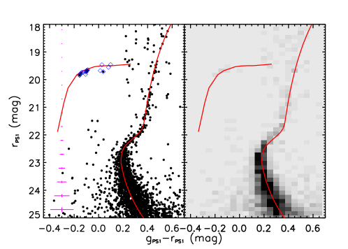
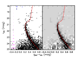
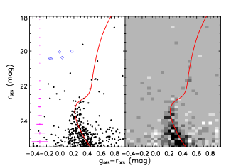
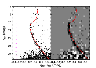
Figures 1 (Sgr II) and 2 (Ret II, Phe II, Tuc III) show the final color magnitude diagrams (CMDs), which include stars within one half-light radius of the center (see Section 3.3). Magenta error bars show the mean photometric errors determined from artificial stars. The error bars are plotted at an arbitrary color for convenience. Blue open diamonds are the blue horizontal-branch star (HB) candidates in our FoV, which are selected within a filter with a color of and a span of mag, centered on the HB sequence of a metal-poor PARSEC isochrone (Bressan et al., 2012). Right panels show background-subtracted binned Hess diagrams, which encode the number density of stars in the selected region. The background is estimated from a field located outside a radius of 12′, well outside the body of each satellite. For Ret II and Tuc III, we use background fields that are northwest and southeast of the centroids because there should be little satellite contamination at these positions, given the position angle and high-ellipticity of Ret II (see Table 3.3) and the orientation of Tuc III stream (see Section 4.4). In Figure 2, overplotted as a red line is a metal-poor Dartmouth isochrone (Dotter et al., 2008), which corresponds to the best-fit Dartmouth isochrone in Section 3.2. In Figure 1, we use the PS1 fiducial for globular cluster NGC 7078 (M15) from Bernard et al. (2014), which is a better fit for Sgr II than any theoretical isochrone. Note that there is not any established DES fiducial for globular clusters, and that is why we display theoretical isochrones in Figure 2. We shift each isochrone and fiducial by the best-fit distance modulus that we derive in Section 3.2.
3.2 Distance
We derive the distance to Sgr II by comparing its CMD with empirical globular cluster fiducials and theoretical isochrones. We use four empirical fiducials determined by Bernard et al. (2014) using the PS1 photometry: NGC 7078 (M15), NGC 6341 (M92), NGC 6205 (M13) and NGC 5272 (M3) with [Fe/H]-2.42, -2.38, -1.60, and -1.50 (Kraft & Ivans, 2003). We assume the distance modulus values of =15.25 for M15, 14.75 for M92, 14.42 for M13, and 15.02 for M3 (Kraft & Ivans, 2003), with an uncertainty of 0.1 mag. Besides these four empirical fiducials, we also use the Dartmouth isochrones with [Fe/H], [/Fe], and a 13.5 Gyr stellar population.
To determine the distance modulus of Sgr II, we follow a very similar methodology as that described in Sand et al. (2009) (see also Walsh et al. 2008). We include all stars with mag within of its center. Each fiducial is shifted through 0.025 mag intervals in from 18.0 to 20.0 mag. In each step, we count the number of stars consistent with the fiducial, taking into account photometric uncertainties. The selection region is defined by two selection boundaries on either side along the color axis at the typical color uncertainty at a given magnitude, as determined via our artificial star tests. We also account for background stars by running the identical procedure in parallel over an appropriately scaled background region offset from Sgr II, counting the number of stars consistent with the fiducial and then subtracting this number from that derived at the position of the dwarf. We derive the best-fit distance modulus when the fiducial gives the maximum number of dwarf stars: 19.250 for M15 (150 stars), 19.125 for M92 (170 stars), 18.675 for M13 (93 stars), 18.700 for M3 (68 stars). Sgr II’s CMD is clearly more consistent with the metal-poor fiducials, i.e., M15 and M92. The Dartmouth isochrone gives =19.225 mag with 112 stars. We use a 100 iteration bootstrap analysis to determine the uncertainties on each fit.
We also derive a distance modulus using the possible blue HBs of Sgr II within our FoV (19 stars). We fit to both of the metal-poor fiducial HB sequences (M15 and M92) by minimizing the sum of the squares of the difference between the data and the fiducial. The best-fit distance modulus from HBs is 19.30 for M15 and 19.26 for M92. We calculate the associated uncertainties via jackknife resampling, which accounts for both the finite number of stars and the possibility of occasional interloper stars. We compute the mean and standard deviation of the derived distance moduli from both methods, i.e., fitting the HB sequence (19.30, 19.26) and counting stars from M15 (19.250), M92 (19.125) and the isochrone (19.225). The mean is adopted as our final distance modulus value, and the standard deviation as our uncertainty. The distance modulus uncertainty of the globular clusters and the uncertainties from both jackknife resampling and our bootstrap analysis are added in quadrature to produce our final quoted uncertainty (see Table 3.3).
We derive the distance to the other satellites by comparing their CMDs with a grid of isochrones from both Bressan et al. (2012) and Dotter et al. (2008), using the star counting technique described above. We use a 13.5 Gyr stellar population with a range of metallicities ([Fe/H], , , , ). Similar to Sgr II, the best-fit distance modulus values are found when the distanced-shifted isochrones give the maximum number of dwarf stars with mag. For Phe II, which has very few RGB stars, we extend the limiting magnitude to mag to capture a larger number of main-sequence stars. The best-fit Dartmouth and PARSEC isochrones are the ones with [Fe/H] and [Fe/H] for Ret II, [Fe/H] and [Fe/H] for Phe II, [Fe/H] and [Fe/H] for Tuc III, respectively. We adopt the mean of the results from these isochrones as our final distance moduli, and their standard deviation as our uncertainty. The uncertainties from our bootstrap analysis are added in quadrature to produce our final quoted uncertainty (see Table 3.3).
3.3 Structural Properties
To constrain the structural parameters of our objects, we fit an exponential profile to the 2D distribution of stars consistent with each satellite by using the maximum likelihood (ML) technique of Martin et al. (2008) as implemented by Sand et al. (2009). In our analysis, we only select stars consistent with the best-fitting Dartmouth isochrone in color-magnitude space after taking into account photometric uncertainties, within our 90% completeness limit (see Table 2). We inflate the uncertainty to 0.1 mag when the photometric errors are mag for the purpose of selecting stars to go into our ML analysis. For Tuc III, a limiting magnitude of mag is used to avoid contamination from field stars and unresolved background galaxies. The resulting structural parameters are summarized in Table 3.3, which includes the central position, half-light radius (), ellipticity () and position angle. The quoted is the best-fit elliptical half-light radius along the semi-major axis. Uncertainties are determined by bootstrap resampling the data 1000 times and recalculating the structural parameters for each resample. We check our results by repeating the calculations with the same set of stars, but with a limit one magnitude brighter. The derived structural parameters using both samples of stars are consistent within the uncertainties.
Recently, Muñoz et al. (2012) presented a suite of simulations of low-luminosity MW satellites under different observing conditions to recover structural parameters within 10% or better of their true values: they suggested a FoV at least three times that of the half-light radius being measured, greater than 1000 stars in the total sample, and a central density contrast of 20 over the background. These conditions are satisfied in our data for all but one satellite, Tuc III. Our sample of Tuc III has 500 stars and a central density contrast of 15; moreover Tuc III is clearly a disrupting system (e.g. Drlica-Wagner et al., 2015; Shipp et al., 2018, and see Section 4.4) whose true structural parameters may be difficult to gauge with our ML technique.
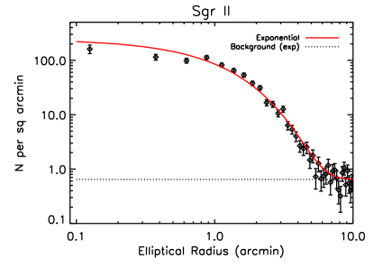
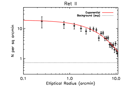
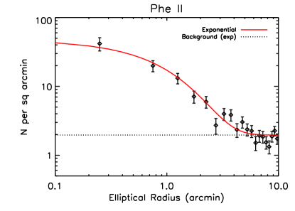
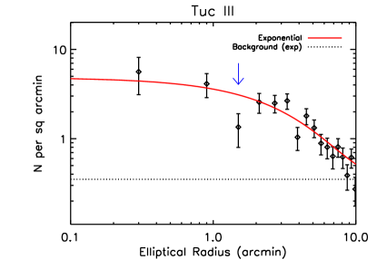
In Figure 3, we show one-dimensional stellar radial profiles, along with our best-fit exponential profile derived from the best-fit two-dimensional stellar distribution. We use elliptical bins based on the parameters from the ML analysis. The one-dimensional representations of the exponential fit and the data are in good agreement, but we also note that parameterized models, condensed to one-dimension, cannot capture a satellite’s potentially complex structure. For Tuc III, there are two bright stars which lead to incompleteness in our star counts, as shown with a blue arrow (see also Figure 4). We also note that the radial density profiles of Ret II and Tuc III do not reach the background level while those of Sgr II and Phe II barely do. This limits our ability to investigate the outer regions of these satellites.
| Parameter | Sgr II | Ret II | Phe II | Tuc III |
|---|---|---|---|---|
| RA (J2000.0) | ||||
| DEC (J2000.0) | ||||
| (mag) | ||||
| Distance (kpc) | ||||
| 222 is the number of stars brighter than mag selected by the best-fit isochrone for each object. | 1502 | 1120 | 162 | 419 |
| (arcmin) | ||||
| (pc) | ||||
| Ellipticity | ||||
| Position Angle (deg) | Unconstrained | |||
| (Ge) | 18.7 | 18.9 | 18.2 | 19.2 |
| () | 1300 | 430 | 1400 | 210 |
| () | 0.2 | 0.4 | 2 | 0.5 |
3.4 Absolute Magnitude
We derive absolute magnitudes for our objects by using the same procedure as in Sand et al. (2009, 2010), as was first described in Martin et al. (2008). First, we build a well-populated CMD (of 20,000 stars), including our completeness and photometric uncertainties, by using the best-fit Dartmouth isochrone (Sgr II and Phe II: [Fe/H]; Ret II and Tuc III: [Fe/H]) and its associated luminosity function with a Salpeter initial mass function. Then, we randomly select the same number of stars from this artificial CMD as was found from our exponential profile fits (over the same magnitude range as was used for the ML analysis). We correct the number of stars of Tuc III for the bin obscured by bright stars, assuming that this bin (highlighted by blue arrow in Figure 3) has a stellar density that lands on the exponential fit. We sum the flux of these stars, and extrapolate the flux of unaccounted stars using the adopted luminosity function. We calculate 1000 realizations in this way, and take the mean as our absolute magnitude and its standard deviation as our uncertainty. To account for the distance modulus uncertainty and the uncertainty on the number of stars, we repeat this operation 100 times, varying the presumed distance modulus and number of stars within their uncertainties, and use the offset from the best-fit value as the associated uncertainty. All of these error terms are then added in quadrature to produce our final uncertainty on the absolute magnitude. We note that the Dartmouth isochrone accounts for red giant branch (RGB) and main sequence stars but not HB sequences. Adding the fluxes of our HB candidates gives the total absolute magnitude of mag for Sgr II, mag for Ret II and mag for Phe II, which we adopt as our final values. For each satellite, the effect of HB candidates on the absolute magnitude is within our quoted uncertainty. Note that Tuc III does not have any HB candidates.
3.5 Extended Structure Search
Given photometric hints that some new MW satellites may be tidally disturbed (e.g., Sand et al., 2009; Muñoz et al., 2010, among others), we search for any sign of tidal interaction, such as streams or other extensions, within our data. We use a matched-filter technique similar to Sand et al. (2012), as was originally described in Rockosi et al. (2002). This method maximizes the signal to noise in possible satellite stars over the background. As signal CMDs, we use the artificial ones that are created in Section 3.4 to derive the absolute magnitudes. For background CMDs, we use stars from a field well outside the body of each satellite. We bin these CMDs into 0.150.15 color-magnitude bins.
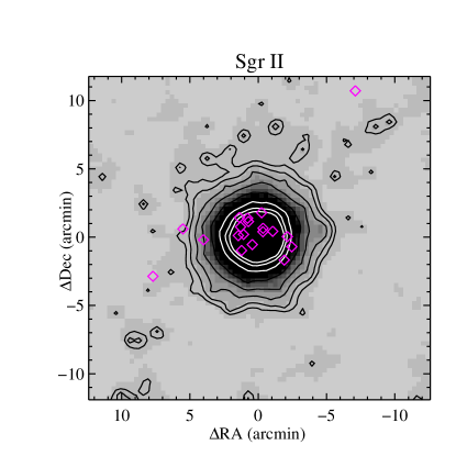
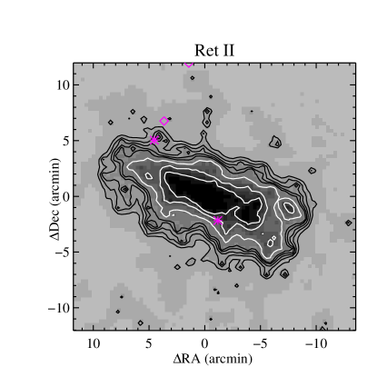
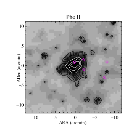
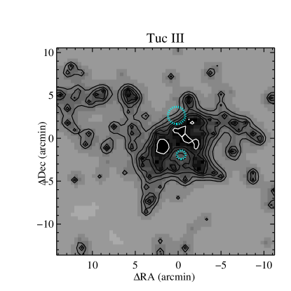
Figure 4 shows our final smoothed matched-filter maps, where we have spatially binned the input data, and smoothed with a Gaussian of width 1.5 times that of the pixel size. Spatial bins for Sgr II and Ret II are 20″, while for Phe II and Tuc III we used spatial pixels of 25″. The background of these smoothed maps is determined using the MMM routine in IDL. The main body of each satellite is clearly visible in each map. Magenta diamonds show blue HB candidates if there are any. In the Tuc III map, scaled cyan circles highlight the position of bright stars and the approximate size of their halos – in these regions our stellar catalogs are compromised, which translates to holes in our spatial maps.
3.6 Neutral Hydrogen Content
We constrain the neutral hydrogen (H I) content of our objects by mining the HI Parkes All-Sky Survey (HIPASS, Barnes et al., 2001; Kalberla & Haud, 2015) and Galactic All-Sky Survey (GASS, McClure-Griffiths et al., 2009) along the lines-of-sight given in Table 3.3. We find no evidence for H I emission within the half-light radii of the objects at heliocentric velocities in the range , beyond that from the H I layer of the MW itself at . We therefore place upper limits on the H I mass of each object, using stellar radial velocity measurements to constrain the search when possible. The resulting and are given in Table 3.3.
The measured stellar radial velocity centroids of Ret II (, Simon et al. 2015) and Tuc III (, Simon et al. 2017) place them within and beyond the range of contaminated by MW H I emission, respectively, at the GASS sensitivity. The upper limit on the H I mass of Ret II derived by Westmeier et al. (2015) using HIPASS (before a for this object was published) is only valid if it is well-separated from the MW H I layer in velocity; this is clearly not the case. We therefore derive a physically meaningful using the GASS data (which, unlike HIPASS, accurately recover large-scale H I emission) at for Ret II, smoothing to a spectral resolution of and adopting this velocity width in the upper limit. Since Tuc III is well-separated from the MW H I layer, we use the more sensitive HIPASS data to derive in a single –wide Hanning-smoothed channel.
Stellar radial velocity measurements for Sgr II and Phe II are not available in the literature. For Sgr II, we compute from HIPASS as described for Tuc III above; for Phe II, we use the upper limit obtained by Westmeier et al. (2015) from reprocessed HIPASS data, adjusting to the distance reported in Table 6. We emphasize that these are valid only if for Sgr II and Phe II are well-separated from MW emission along their respective lines-of-sight. Using the GASS data to identify the velocity ranges contaminated by the MW, we find that is valid for Sgr II if it has or , and is valid for Phe II or .
The upper limits on the gas richness for Sgr II, Ret II and Tuc III imply that these objects are gas-poor, while for Phe II does not rule out the possibility of a gas reservoir similar to that of gas-rich galaxies in the Local Volume (Huang et al., 2012; Bradford et al., 2015). The general lack of H I in these objects is consistent with their location within the virial radius of the MW and M31, within which all low-mass satellites are devoid of gas (e.g. Grcevich & Putman, 2009; Spekkens et al., 2014; Westmeier et al., 2015).
4 DISCUSSION
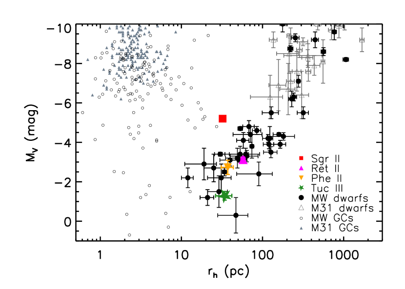
Figure 5 displays the absolute magnitude () vs. half-light radius () of our objects in the context of M31 and MW satellites. Small filled gray triangles are M31 globular clusters from Strader et al. (2011), and open gray triangles are M31 satellite galaxies from McConnachie (2012). Small open black circles represent MW globular clusters from the Harris (2010) catalog, supplemented by more recent discoveries (Belokurov et al., 2010; Muñoz et al., 2012; Balbinot et al., 2013; Kim & Jerjen, 2015; Kim et al., 2015b, 2016; Laevens et al., 2014). Filled black circles show MW dwarfs from McConnachie (2012), including recently discovered MW dwarf candidates (Kim et al., 2016; Drlica-Wagner et al., 2015; Koposov et al., 2015a; Kim & Jerjen, 2015; Bechtol et al., 2015; Torrealba et al., 2016; Laevens et al., 2015; Homma et al., 2016, 2018; Drlica-Wagner et al., 2016; Koposov et al., 2018; Carlin et al., 2017). Our objects are displayed with a filled red square (Sgr II), filled magenta triangle (Ret II), filled yellow upside down triangle (Phe II), and filled green star (Tuc III). Sgr II stands out with its intermediate position between the loci of dwarf galaxies and globular clusters in the size-luminosity plane. We discuss each satellite’s derived properties in detail in the following subsections.
4.1 Sgr II
Our deep photometry provides robust constraints on the structural parameters of Sgr II, and our results are consistent with the discovery analysis of Laevens et al. (2015) within the uncertainties. The CMD of Sgr II (Figure 1) has well-defined features: a narrow RGB and a clear main sequence turnoff (MSTO), with several blue HB candidates. In Figure 4, magenta diamonds show the spatial position of the HB candidates, most of which are centrally concentrated around Sgr II. Overall, the CMD is consistent with an old stellar population with [Fe/H]2.
Sgr II occupies an interesting place in the size-luminosity plane (see Figure 5), as it sits in an intermediate position between the loci of dwarf galaxies and globular clusters. Nonetheless, there are several globular clusters with large half-light radii ( pc) and an absolute magnitude of mag that occupy a similar region in parameter space (see Figure 5). They are mostly distant, and the most metal poor among them (NGC 5053) has [Fe/H] (Harris, 2010), a value that is consistent with the photometric metallicity of Sgr II. Adding to this, Sgr II is very round, with 0.1, which is consistent with the bulk of MW GCs, although there are definite dwarf galaxies with similar ellipticities (for instance, Leo II; Coleman et al., 2007a).
The ensemble properties of Sgr II (i.e., distance, luminosity, and size) are comparable to that of Palomar 14 (Pal 14), which is one of the most distant ( kpc), faint ( mag), and diffuse ( pc) outer Galactic halo globular clusters (Sollima et al., 2011)333Note that in Figure 5 we plot the properties of MW globular clusters from Harris (2010), which report pc and mag for Pal 14.. Similar to Sgr II, the CMD of Pal 14 presents a narrow RGB (Sollima et al., 2011). However, Sgr II is more metal-poor than Pal 14 ([Fe/H]). Based on its existing tidal tail, Pal 14 was suggested to be a part of a stream consisting of the Fornax dSph and globular cluster Palomar 15 (Sollima et al., 2011).
A population of extended, diffuse star clusters have recently been discovered around M31 (Huxor et al., 2014) with roughly similar properties to Sgr II. Most of these systems are far from M31 itself (30 kpc), and many appear to be associated with streams (Chapman et al., 2008; Forbes & Bridges, 2010; Mackey et al., 2010). This supports the picture described by Laevens et al. (2015) in which Sgr II was brought into the MW halo along with the Sgr stream, and similar to numerous other MW and M31 GCs (e.g. Law & Majewski, 2010; Mackey et al., 2013).
Despite the strong hints presented above that Sgr II is likely an extended globular cluster, ultimately spectroscopic follow up is necessary to determine its true nature.
4.2 Ret II
In Figure 2, the CMD of Ret II shows a well-defined main sequence, with several blue HB candidates which trace its density contours. Two of our candidates (shown with magenta stars in Figure 4) are the confirmed members of Ret II (Simon et al., 2015), based on their velocities. We note that other two were not studied by Simon et al. (2015). Our distance measurement (D=321 kpc) is consistent with both independent discovery analyses (Bechtol et al., 2015; Koposov et al., 2015a). Our ML analysis suggests a similar value for its half-light radius ( pc) to the result of Bechtol et al. (2015, pc), and this is also marginally consistent with the result444Koposov et al. (2015a) reported the azimuthally averaged half-light radius of 32 pc. Their value after correcting for the ellipticity is pc of Koposov et al. (2015a). Our absolute magnitude measurement () is in between the results of Koposov et al. (2015a, ) and Bechtol et al. (2015, ). Ret II is among the most elongated of the MW satellites with 0.6, comparable to Hercules (0.7) and Ursa Major I (0.8), both of which are at 100 kpc (see Table 7 of Sand et al. 2012). Therefore, Ret II is the most elongated nearby dwarf galaxy currently known for its luminosity range. In spite of its elongated nature, our density map does not show any clear sign of tidal features within our FoV (see Figure 4). Deep wide-field observations of Ret II are necessary to truly search for signs of extended structure.
Ret II lands directly on the locus defined by MW ultra-faint dwarf galaxies of similar luminosity (see Figure 5); spectroscopic follow-up (Simon et al., 2015; Walker et al., 2015; Koposov et al., 2015b) confirmed that it is a MW ultra-faint dwarf galaxy based on the velocities and metallicities of its stars. They found that Ret II is strongly dark matter dominated and one of the most metal-poor galaxies known with a mean metallicity of [Fe/H]. As expected from these studies, an old metal-poor Dartmouth isochrone ([Fe/H], [/Fe], 13.5 Gyr) provides the best fit to the features of its CMD at our measured distance (see Figure 2).
A tentative gamma-ray detection associated with Ret II (at the level; Geringer-Sameth et al., 2015), led to excitement that a signal from annihilating dark matter was found, but this detection is not seen by all of the searching teams (see Drlica-Wagner et al., 2015). Using the photometric analysis of Bechtol et al. (2015), Simon et al. (2015) conclude that Segue 1, Ursa Major II and Coma Berenices, which possess larger J-factors, are more promising gamma-ray targets than Ret II. Using our photometric analysis and the scaling relation of Pace & Strigari (2018), we find the same value for the J-factor and confirm their conclusion.
4.3 Phe II
The CMD features of Phe II are much clearer in the Hess diagram, which accounts for the contaminating background stars (see Figure 2). Phe II has a sparsely populated RGB, with a potential population of blue HBs outside our half-light radius (see Figure 4).
The structural parameters of Phe II are not well-constrained in the discovery analyses (Bechtol et al., 2015; Koposov et al., 2015a). Our deep photometry provides robust constraints on these parameters, which mostly agree well with the results from Koposov et al. (2015a), within the uncertainties. Compared to their estimations, our ML analysis suggests a similar size ( pc versus 555Koposov et al. (2015a) reported the azimuthally averaged half-light radius of 26 pc. This is their value after correcting for the ellipticity. pc) and a slightly rounder shape ( versus ) with similar luminosity ( versus ) for Phe II. We note our absolute magnitude is fainter than that in Bechtol et al. (2015) (), however their value would be if shifted by our distance modulus (). In Figure 5, it lands directly on the locus defined by other MW ultra-faint dwarf galaxies of similar luminosity. Judging from the ellipticity and position in the size-luminosity plane, it is likely that Phe II is a dwarf galaxy.
4.4 Tuc III
Our deep photometry of Tuc III reveals a well-defined narrow main sequence consistent with old, metal-poor stellar populations, as expected from the spectroscopic metallicity measurement ([Fe/H], Simon et al. 2017). There are no HB candidates within our FoV, both within our Magellan photometric catalog (which saturates at 18 mag) and the DES catalog, which goes to brighter magnitudes (Drlica-Wagner et al., 2015).
Tuc III is known to host a stellar stream extending at least from its core (Drlica-Wagner et al., 2015; Shipp et al., 2018). Despite our narrow FoV, and the likelihood that it is contaminated with Tuc III stars throughout, there is still evidence for the stream in our stellar density map (see Figure 4). The presence of bright stars in our field (cyan circles) causes some irregularities in the contours of the satellite body near its center. Despite the existence of a stellar stream, Drlica-Wagner et al. (2015) suggest a relatively low ellipticity for Tuc III. Our ML analysis gives an ellipticity of with a major-axis position angle of . Compared to the discovery analysis ( pc, ), our photometry suggests a similar size ( pc) within the uncertainties, but fainter absolute magnitude (). The stellar stream together with the narrow FoV and presence of bright stars makes it hard to obtain a robust estimate of Tuc III’s structural parameters, therefore our results should be used with caution.
Spectroscopic follow-up (Simon et al., 2017) has been unable to conclusively determine Tuc III’s dynamical status and dark matter content. Compared to any known dwarf galaxy, they found a smaller metallicity dispersion and likely a smaller velocity dispersion for Tuc III, and tentatively suggested that it is the tidally-stripped remnant of a dark matter-dominated dwarf galaxy. Moreover, its location in the size-luminosity plane favors a ultra-faint dwarf galaxy interpretation (see Figure 5), comparable to Segue I (, pc) and Triangulum II (, pc), both of which have been suggested to be tidally stripped (e.g., Niederste-Ostholt et al., 2009; Kirby et al., 2017).
5 SUMMARY AND CONCLUSIONS
We have presented deep Magellan/Megacam photometric follow-up observations of new MW satellites Sgr II, Ret II, Phe II, and Tuc III. Our photometry reaches 2-3 mag deeper than the original discovery data for each object, and allows us to revisit the distance, structural properties, and luminosity measurements. An archival analysis allowed us to place HI gas mass limits on each system, which are all devoid of gas as expected for their location within the virial radius of the MW (e.g. Spekkens et al., 2014).
Sgr II stands in an interesting location in the size-luminosity plane, just between the loci of dwarf galaxies and globular clusters. However, the ensemble of its structural parameters is more consistent with a globular cluster classification. In particular, many of its physical properties are comparable to those of Pal 14. Spectroscopic follow up is necessary to determine its true nature.
Two independent discovery analyses found different values for the structural parameters of Ret II and Phe II. Our deep photometry resolves this inconsistency, and provides robust constraints on these parameters. We find for Ret II and for Phe II, with corresponding half-light radii of pc and pc. Ret II and Phe II therefore land directly on the locus defined by MW ultra-faint dwarf galaxies of similar luminosity. Ret II is the most elongated nearby dwarf galaxy currently known for its luminosity range, and it is more likely that Phe II is a dwarf galaxy than a star cluster.
Tuc III is extremely faint with , and compact ( pc). It is apparently made up of an old, metal-poor stellar population, as expected from its measured spectroscopic metallicity of [Fe/H] (Simon et al., 2017). Our photometry suggests that Tuc III is a tidally-disrupted dwarf galaxy.
Finally, we search for any clear sign of extended structure for these satellites (see Figure 4). We find no evidence for structural anomalies or tidal disruption in Sgr II and Phe II. In spite of its apparent high ellipticity, Ret II also does not show any firm evidence of extra-tidal material outside the satellite. The stellar density map of Tuc III is of particular interest, because it is known to be associated with a stellar stream. Our deep imaging allows us to map the connection between the stellar steam and the body of Tuc III. However, deep wide-field observations, in particular for Ret II and Tuc III, are necessary to definitively investigate the outer regions of these systems.
References
- Adén et al. (2009) Adén, D., Wilkinson, M. I., Read, J. I., et al. 2009, ApJ, 706, L150
- Balbinot et al. (2013) Balbinot, E., Santiago, B. X., da Costa, L., et al. 2013, ApJ, 767, 101
- Baltz et al. (2008) Baltz, E. A., Berenji, B., Bertone, G., et al. 2008, J. Cosmology Astropart. Phys, 7, 013
- Barnes et al. (2001) Barnes, D. G., Staveley-Smith, L., de Blok, W. J. G., et al. 2001, MNRAS, 322, 486
- Bechtol et al. (2015) Bechtol, K., Drlica-Wagner, A., Balbinot, E., et al. 2015, ApJ, 807, 50
- Belokurov et al. (2014) Belokurov, V., Irwin, M. J., Koposov, S. E., et al. 2014, MNRAS, 441, 2124
- Belokurov et al. (2010) Belokurov, V., Walker, M. G., Evans, N. W., et al. 2010, ApJ, 712, L103
- Bergström & Snellman (1988) Bergström, L., & Snellman, H. 1988, Phys. Rev. D, 37, 3737
- Bernard et al. (2014) Bernard, E. J., Ferguson, A. M. N., Schlafly, E. F., et al. 2014, MNRAS, 442, 2999
- Bertin & Arnouts (1996) Bertin, E., & Arnouts, S. 1996, A&AS, 117, 393
- Bradford et al. (2015) Bradford, J. D., Geha, M. C., & Blanton, M. R. 2015, ApJ, 809, 146
- Bressan et al. (2012) Bressan, A., Marigo, P., Girardi, L., et al. 2012, MNRAS, 427, 127
- Carlin et al. (2017) Carlin, J. L., Sand, D. J., Muñoz, R. R., et al. 2017, AJ, 154, 267
- Chambers et al. (2016) Chambers, K. C., Magnier, E. A., Metcalfe, N., et al. 2016, ArXiv e-prints, arXiv:1612.05560
- Chapman et al. (2008) Chapman, S. C., Ibata, R., Irwin, M., et al. 2008, MNRAS, 390, 1437
- Coleman et al. (2007a) Coleman, M. G., Jordi, K., Rix, H.-W., Grebel, E. K., & Koch, A. 2007a, AJ, 134, 1938
- Coleman et al. (2007b) Coleman, M. G., de Jong, J. T. A., Martin, N. F., et al. 2007b, ApJ, 668, L43
- Collins et al. (2017) Collins, M. L. M., Tollerud, E. J., Sand, D. J., et al. 2017, MNRAS, 467, 573
- Conn et al. (2018a) Conn, B. C., Jerjen, H., Kim, D., & Schirmer, M. 2018a, ApJ, 852, 68
- Conn et al. (2018b) —. 2018b, ApJ, 857, 70
- Crnojević et al. (2016) Crnojević, D., Sand, D. J., Zaritsky, D., et al. 2016, ApJ, 824, L14
- DES Collaboration (2018) DES Collaboration. 2018, ArXiv e-prints, arXiv:1801.03181
- Dotter et al. (2008) Dotter, A., Chaboyer, B., Jevremović, D., et al. 2008, ApJS, 178, 89
- Drlica-Wagner et al. (2015) Drlica-Wagner, A., Bechtol, K., Rykoff, E. S., et al. 2015, ApJ, 813, 109
- Drlica-Wagner et al. (2016) Drlica-Wagner, A., Bechtol, K., Allam, S., et al. 2016, ApJ, 833, L5
- Fitzpatrick (1999) Fitzpatrick, E. L. 1999, PASP, 111, 63
- Flewelling et al. (2016) Flewelling, H. A., Magnier, E. A., Chambers, K. C., et al. 2016, ArXiv e-prints, arXiv:1612.05243
- Forbes & Bridges (2010) Forbes, D. A., & Bridges, T. 2010, MNRAS, 404, 1203
- Garling et al. (2018) Garling, C., Willman, B., Sand, D. J., et al. 2018, ApJ, 852, 44
- Geringer-Sameth et al. (2015) Geringer-Sameth, A., Walker, M. G., Koushiappas, S. M., et al. 2015, Physical Review Letters, 115, 081101
- Grcevich & Putman (2009) Grcevich, J., & Putman, M. E. 2009, ApJ, 696, 385
- Gunn et al. (1978) Gunn, J. E., Lee, B. W., Lerche, I., Schramm, D. N., & Steigman, G. 1978, ApJ, 223, 1015
- Harris (2010) Harris, W. E. 2010, ArXiv e-prints, arXiv:1012.3224
- Homma et al. (2016) Homma, D., Chiba, M., Okamoto, S., et al. 2016, ApJ, 832, 21
- Homma et al. (2018) —. 2018, PASJ, 70, S18
- Hooper & Linden (2015) Hooper, D., & Linden, T. 2015, J. Cosmology Astropart. Phys, 9, 016
- Huang et al. (2012) Huang, S., Haynes, M. P., Giovanelli, R., & Brinchmann, J. 2012, ApJ, 756, 113
- Huxor et al. (2014) Huxor, A. P., Mackey, A. D., Ferguson, A. M. N., et al. 2014, MNRAS, 442, 2165
- Kalberla & Haud (2015) Kalberla, P. M. W., & Haud, U. 2015, A&A, 578, A78
- Kim & Jerjen (2015) Kim, D., & Jerjen, H. 2015, ApJ, 799, 73
- Kim et al. (2015a) Kim, D., Jerjen, H., Mackey, D., Da Costa, G. S., & Milone, A. P. 2015a, ApJ, 804, L44
- Kim et al. (2016) —. 2016, ApJ, 820, 119
- Kim et al. (2015b) Kim, D., Jerjen, H., Milone, A. P., Mackey, D., & Da Costa, G. S. 2015b, ApJ, 803, 63
- Kirby et al. (2017) Kirby, E. N., Cohen, J. G., Simon, J. D., et al. 2017, ApJ, 838, 83
- Koposov et al. (2017) Koposov, S. E., Belokurov, V., & Torrealba, G. 2017, MNRAS, 470, 2702
- Koposov et al. (2015a) Koposov, S. E., Belokurov, V., Torrealba, G., & Evans, N. W. 2015a, ApJ, 805, 130
- Koposov et al. (2015b) Koposov, S. E., Casey, A. R., Belokurov, V., et al. 2015b, ApJ, 811, 62
- Koposov et al. (2018) Koposov, S. E., Walker, M. G., Belokurov, V., et al. 2018, ArXiv e-prints, arXiv:1804.06430
- Kraft & Ivans (2003) Kraft, R. P., & Ivans, I. I. 2003, PASP, 115, 143
- Laevens et al. (2014) Laevens, B. P. M., Martin, N. F., Sesar, B., et al. 2014, ApJ, 786, L3
- Laevens et al. (2015) Laevens, B. P. M., Martin, N. F., Bernard, E. J., et al. 2015, ApJ, 813, 44
- Landsman (1993) Landsman, W. B. 1993, in Astronomical Society of the Pacific Conference Series, Vol. 52, Astronomical Data Analysis Software and Systems II, ed. R. J. Hanisch, R. J. V. Brissenden, & J. Barnes, 246
- Law & Majewski (2010) Law, D. R., & Majewski, S. R. 2010, ApJ, 718, 1128
- Mackey et al. (2010) Mackey, A. D., Huxor, A. P., Ferguson, A. M. N., et al. 2010, ApJ, 717, L11
- Mackey et al. (2013) —. 2013, MNRAS, 429, 281
- Magnier et al. (2016) Magnier, E. A., Schlafly, E. F., Finkbeiner, D. P., et al. 2016, ArXiv e-prints, arXiv:1612.05242
- Martin et al. (2008) Martin, N. F., de Jong, J. T. A., & Rix, H.-W. 2008, ApJ, 684, 1075
- Martin et al. (2015) Martin, N. F., Nidever, D. L., Besla, G., et al. 2015, ApJ, 804, L5
- McClure-Griffiths et al. (2009) McClure-Griffiths, N. M., Pisano, D. J., Calabretta, M. R., et al. 2009, ApJS, 181, 398
- McConnachie (2012) McConnachie, A. W. 2012, AJ, 144, 4
- McLeod et al. (2015) McLeod, B., Geary, J., Conroy, M., et al. 2015, PASP, 127, 366
- McLeod et al. (2000) McLeod, B. A., Conroy, M., Gauron, T. M., Geary, J. C., & Ordway, M. P. 2000, in Further Developments in Scientific Optical Imaging, ed. M. B. Denton, 11
- Muñoz et al. (2012) Muñoz, R. R., Geha, M., Côté, P., et al. 2012, ApJ, 753, L15
- Muñoz et al. (2010) Muñoz, R. R., Geha, M., & Willman, B. 2010, AJ, 140, 138
- Niederste-Ostholt et al. (2009) Niederste-Ostholt, M., Belokurov, V., Evans, N. W., et al. 2009, MNRAS, 398, 1771
- Pace & Strigari (2018) Pace, A. B., & Strigari, L. E. 2018, ArXiv e-prints, arXiv:1802.06811
- Rockosi et al. (2002) Rockosi, C. M., Odenkirchen, M., Grebel, E. K., et al. 2002, AJ, 124, 349
- Roderick et al. (2015) Roderick, T. A., Jerjen, H., Mackey, A. D., & Da Costa, G. S. 2015, ApJ, 804, 134
- Sand et al. (2009) Sand, D. J., Olszewski, E. W., Willman, B., et al. 2009, ApJ, 704, 898
- Sand et al. (2010) Sand, D. J., Seth, A., Olszewski, E. W., et al. 2010, ApJ, 718, 530
- Sand et al. (2012) Sand, D. J., Strader, J., Willman, B., et al. 2012, ApJ, 756, 79
- Schlafly & Finkbeiner (2011) Schlafly, E. F., & Finkbeiner, D. P. 2011, ApJ, 737, 103
- Schlegel et al. (1998) Schlegel, D. J., Finkbeiner, D. P., & Davis, M. 1998, ApJ, 500, 525
- Shipp et al. (2018) Shipp, N., Drlica-Wagner, A., Balbinot, E., et al. 2018, ArXiv e-prints, arXiv:1801.03097
- Simon et al. (2015) Simon, J. D., Drlica-Wagner, A., Li, T. S., et al. 2015, ApJ, 808, 95
- Simon et al. (2017) Simon, J. D., Li, T. S., Drlica-Wagner, A., et al. 2017, ApJ, 838, 11
- Skrutskie et al. (2006) Skrutskie, M. F., Cutri, R. M., Stiening, R., et al. 2006, AJ, 131, 1163
- Sollima et al. (2011) Sollima, A., Martínez-Delgado, D., Valls-Gabaud, D., & Peñarrubia, J. 2011, ApJ, 726, 47
- Spekkens et al. (2014) Spekkens, K., Urbancic, N., Mason, B. S., Willman, B., & Aguirre, J. E. 2014, ApJ, 795, L5
- Stetson (1994) Stetson, P. B. 1994, PASP, 106, 250
- Strader et al. (2011) Strader, J., Caldwell, N., & Seth, A. C. 2011, AJ, 142, 8
- Torrealba et al. (2016) Torrealba, G., Koposov, S. E., Belokurov, V., et al. 2016, MNRAS, 463, 712
- Torrealba et al. (2018) Torrealba, G., Belokurov, V., Koposov, S. E., et al. 2018, MNRAS, 475, 5085
- Van Der Walt et al. (2011) Van Der Walt, S., Colbert, S. C., & Varoquaux, G. 2011, ArXiv e-prints, arXiv:1102.1523
- Walker et al. (2015) Walker, M. G., Mateo, M., Olszewski, E. W., et al. 2015, ApJ, 808, 108
- Walsh et al. (2008) Walsh, S. M., Willman, B., Sand, D., et al. 2008, ApJ, 688, 245
- Westmeier et al. (2015) Westmeier, T., Staveley-Smith, L., Calabretta, M., et al. 2015, MNRAS, 453, 338