Quasars probing quasars X: The quasar pair spectral database

Abstract

The rare close projection of two quasars on the sky provides the opportunity to study the host galaxy environment of a foreground quasar in absorption against the continuum emission of a background quasar. For over a decade the "Quasars probing quasars" series has utilized this technique to further the understanding of galaxy formation and evolution in the presence of a quasar at $z>2$, resolving scales as small as a galactic disc and from bound gas in the circumgalactic medium to the diffuse environs of intergalactic space. Presented here, is the public release of the quasar pair spectral database utilized in these studies. In addition to projected pairs at $z>2$, the database also includes quasar pair members at $z<2$, gravitational lens candidates and quasars closely separated in redshift that are useful for small-scale clustering studies. In total the database catalogs 5627 distinct objects, with 4083 lying within 5^′of at least one other source. A spectral library contains 3582 optical and near-infrared spectra for 3028 of the cataloged sources. As well as reporting on 54 newly discovered quasar pairs, we outline the key contributions made by this series over the last ten years, summarize the imaging and spectroscopic data used for target selection, discuss the target selection methodologies, describe the database content and explore some avenues for future work. Full documentation for spectral database, including download instructions are supplied at http://specdb.readthedocs.io/en/latest/

1 Introduction

An understanding of the processes by which galaxies accrete, expel and recycle gas is as essential to a complete theory of galaxy evolution as population demographics and star formation. At its largest scales, the Universe is seen as a living network of filaments blossoming with clusters and galaxies at their intersections. This "Cosmic web" contains 90 percent of all the baryonic material in the Universe and supplies the fuel for galaxy formation along its filaments. The journey of this gas into the interstellar medium (ISM) occurs through the circumgalactic medium (CGM), a gravitationally bound gas reservoir, distinct from the ISM but contained within a region similar in extent to a galaxy’s own virial radius. In their recent review, Tumlinson et al. (2017) liken the CGM to a galactic utility provider, acting as the galactic fuel tank, waste dump and recycling center simultaneously.

The CGM is diffuse and therefore difficult to detect in emission, and has traditionally received less attention than the ISM and the intergalactic medium (IGM). However, interest in the CGM has undergone somewhat of a revolution in recent years. Galactic gas flows, which by necessity must pass through the CGM, appear to be at the heart of a myriad of unresolved and compelling issues including the “missing baryon” problem (e.g. Keeney et al., 2017), the metal census (e.g. Peeples et al., 2014), the quenching of star formation in passive galaxies and the perpetuation of star formation in star forming galaxies (the so called red-blue dichotomy e.g. Bordoloi et al., 2011; Borthakur et al., 2016).

Advances in the modeling of galactic flows has prompted large strides forward in the observational capabilities to detect them, notably with the Cosmic Origins Spectrograph (COS; Tumlinson et al., 2013; Werk et al., 2013) on the Hubble Space Telescope (HST). Evidence for accretion flows comes from line widths in HI and various other species, which reveal velocity dispersions in halo gas that show it to be bound (e.g. Tumlinson et al., 2013; Bordoloi et al., 2014; Ho et al., 2017). In the Milky Way, unmistakable evidence for accretion comes in the form of blueshifted high velocity clouds (HVCs) (e.g. Sembach et al., 2004; Lehner & Howk, 2011). In other galaxies the evidence has been more difficult to ascertain presumably because individual flows contain insufficient mass or are too diffuse or both (Rubin et al., 2012). There are a handful of examples in which diffuse gas has been detected in emission around other galaxies (Cantalupo et al., 2014; Martin et al., 2014; Hennawi et al., 2015; Fumagalli et al., 2017) but for the most part the community has relied on absorption line spectroscopy (Rubin et al., 2012; Bouché et al., 2016; Wiseman et al., 2017).

On the other hand observations of pristine gas in the IGM are rare (Fumagalli et al., 2011) and the metalicity of the gas in all phases of the CGM (Tumlinson et al., 2013; Peeples et al., 2014; Prochaska et al., 2017) is a sure indication that it has at some point passed through the ISM. This evokes a picture in which a significant amount of accreted material is recycled, blown out of the ISM and into galactic halos via feedback-triggered outflows. The evidence for outflows is large (Steidel et al., 2010; Rubin et al., 2014; Fox et al., 2015; Wiseman et al., 2017). What is less well known is how outflows interact with the CGM, and beyond, to transport processed matter and energy, and to what extent these processed materials are recycled in subsequent star formation.

The extensive progress of this field in recent years is examined comprehensively in a number of recent reviews (Putman et al., 2012; Tumlinson et al., 2017; Fox & Davé, 2017). However a complete picture of the CGM in the context of galaxy evolution is unachievable without broadening the discussion towards the extreme and evanescent phases of galaxy evolution such as nuclear starbursts, mergers and active galaxies or quasars. The latter has been the subject of a series of nine papers known as the Quasars Probing Quasars (QPQ) project (Hennawi et al., 2006b; Hennawi & Prochaska, 2007; Prochaska & Hennawi, 2009; Hennawi & Prochaska, 2013; Prochaska et al., 2013a, b, 2014; Lau et al., 2016, 2017, henceforth QPQ1-QPQ9). Just as the Cosmic web or a galactic halo can be observed in absorption against the continuum emission of a distant quasar, so too can the CGM of a quasar host when a background quasar is projected close to the line of sight of a foreground quasar. This is in fact the idea behind the QPQ project, which aims to elucidate the CGM in the massive $M\approx 10^{12.5}\,M_{\odot}$ halos that host quasars at $z\gtrsim 2$ (e.g. Eftekharzadeh et al., 2015).

A reoccurring conclusion throughout the QPQ series is that a quasar’s ionizing continuum illuminates surrounding gas in an anisotropic fashion. Excess absorbers are found transverse to quasar sight lines (QPQ1) and the quasar-absorber clustering signal measured in transverse directions has been shown to over predict the number of absorbers in line of sight directions by several times (QPQ2). This result holds to $\mathrm{Mpc}$ scales (QPQ6) and beyond (Font-Ribera et al., 2013, Sorini et al. 2018, in prep.). Furthermore, if this cool gas were to be illuminated by the quasar radiation field then it should emit Ly$\alpha$ photons, either from fluorescent recombinations, resonant scattering, or by Ly$\alpha$ cooling radiation. This has only rarely been found on large scales (QPQ4; Cantalupo et al. 2014; Martin et al. 2014; Hennawi et al. 2015). Other lines of inquiry have failed to detect the transverse proximity effect in background quasar spectra despite numerous attempts (Fernandez-Soto et al., 1995; Liske & Williger, 2001; Schirber et al., 2004; Croft, 2004; Prochaska et al., 2013a).

Large covering fractions of HI extend to impact parameters of $R_{\perp}\lesssim 200\,\mathrm{kpc}$ likely coinciding with the virial radii of halos (; ; ; ). This gas represents up to a third of the total baryonic mass within the CGM, approaching the mass of baryons in the ISM (QPQ7). Beyond $R_{\perp}\gtrsim 500\,\mathrm{kpc}$ the mass of cool gas remains substantial. If it is possible to generalize these findings to all coeval massive galaxies, then a significant amount of all optically thick gas is found within the extended regions around massive galaxies at $z\approx 2$ (QPQ6). Indeed, this phenomenon has no obvious affinity with coeval galaxy populations in other mass regimes (QPQ7) and must surely indicate a divergence of evolutionary processes.

Clues to the provenance of this cool halo gas can be explored via its metal content. Incidences of low-ion metal absorption systems follow closely with the results of HI above, i.e. the gas is enriched out to impact parameters of at least $\mathrm{1\,Mpc}$ and shows the strongest signatures of metal enrichment at $R_{\perp}\lesssim 200\,\mathrm{kpc}$ (; ; ; ). Stacked spectra reveal average profiles of both low and high ions with systematically larger equivalent widths than any other known galaxy population (QPQ7). Strong signatures of $\alpha$-elements implicate core-collapse supernovae as the progenitors of this gas and point to star formation histories similar to massive ellipticals, which are thought to be the modern-day descendants of quasars (; ). This may link the enrichment of the CGM in quasar hosts at least in part to their own ISM but poses further questions regarding transport mechanisms.

Both quasar and star formation feedback are invoked as the transport mechanisms required to move gas out of the ISM and into the CGM. However QPQ finds no obvious evidence for any single dominant process. While kinematics are extreme and in some cases suggestive of violent outflow (; ), on the whole there is no need to appeal to anything beyond the gravitationally supported dynamics expected of massive halos (; ). Simple arguments concerning timescales and energetics show that episodes of quasar activity are insufficient to place metals at $\sim\mathrm{Mpc}$ distances within a single duty cycle (; ). Furthermore cool gas is present, albeit in lower quantities, in the halos of quiescent galaxy populations so ongoing quasar activity is not a prerequisite for its existence. On the other hand the average gas covering fraction may be correlated with quasar bolometric luminosity (Johnson et al., 2015), making it difficult to argue against the connection between cool halo gas and quasar activity. Far from ruling out quasar feedback as a transport mechanism completely, it is more appealing to invoke it as an intermittent agent operating on $\sim 100\,\mathrm{kpc}$ scales.

Outflows supported by star formation feedback are found in a variety galaxy populations across time (Pettini et al., 1998; Martin, 2005; Weiner et al., 2009; Rubin et al., 2014). Ongoing star formation however, does not appear to be precondition of a cool enriched CGM. Early type galaxies contain a large reservoir of cool enriched halo gas (Thom et al., 2012) and there is scant evidence to link the strength or prevalence of optically-thick absorbers to star formation rate (QPQ7). Indeed $z\sim 2$ quasar hosts do not show evidence for increased star formation (Rosario et al., 2013; Stanley et al., 2017). Furthermore the large impact parameters to which cool gas extends puts it beyond the influence of any single star formation episode. The presence of heavy elements in the CGM serves as strong evidence that it has at some point passed through the ISM, but as with quasar feedback this is likely to happen over integrated episodes limited to $\sim 100\,\mathrm{kpc}$ scales.

The presence of heavy elements in the cool halo gas on $\mathrm{Mpc}$ scales means that it cannot be entirely explained by accretion of pristine gas from the cosmic web. Rather it may arise from galactic winds driven by star formation in low-mass satellite galaxies that deposit their metals in cosmic filaments. Modeling of these processes has begun to be able to match the covering fractions of cool gas seen in observations (Faucher-Giguère et al., 2016), which alleviates the need for feedback processes in the host galaxy to act at these distances.

The QPQ series has contributed to a boom in the understanding of the CGM in the massive galaxies that host quasars at $z>2$. To facilitate this work the project has put together a database of over 2000 projected quasar pairs with transverse separations at foreground quasar redshifts ranging from between tens of physical kpc to a few Mpc. Equivalently the database probes scales as small as a galactic disc, to unbound gas in the surrounding IGM, to everything in between. The QPQ collaboration here presents its extensive database of quasar pairs and their spectra. This submission adopts the $\Lambda$CDM cosmology of the Planck Collaboration et al. (2016) and reports all magnitudes on the AB system. Section 2 recalls the basic principles behind the QPQ experiment, section 3 discusses the selection of quasar pairs in spectroscopic redshift surveys, section 4 discusses quasar pair selection in imaging data, section 5 presents recent results from the latest QPQ quasar pair search using ATLAS, SDSS and WISE imaging, section 6 describes the content and architecture of the quasar pair catalog and accompanying spectral database and section 7 provides a summary of this submission and lays out some avenues for the future exploitation of the QPQ database.

2 The Experiment

To begin, it is useful to briefly review the basic principle behind the QPQ experiment. The upper panel of Figure 1 shows the projected quasar pair J1204+0221 in SDSS (Sloan Digital Sky Survey; York et al., 2000) imaging. The pair members are separated by an angular distance of $\theta\simeq 13.28^{\prime\prime}$ on the sky and are located at foreground and background redshifts of $z=2.44$ and $z=2.53$ respectively. From the adopted cosmology it follows that the sightline of the background quasar passes the foreground quasar at a transverse distance of $R_{\perp}\simeq 110\,\mathrm{pkpc}$. On their way to the observer, background quasar photons are absorbed and scattered by gas associated with the foreground quasar’s halo and may ionize HI and other atomic species. The absorption features are seen as electronic transitions, primarily at far-ultra-violet (UV) rest-frame energies, in the spectrum of the background quasar at transition wavelengths corresponding to the redshift of the absorbing gas. This is shown in the lower panel, where Ly$\alpha$ absorption is clearly seen in the background spectrum at the redshift of the foreground quasar. This is accompanied by a series of labeled metal transitions.

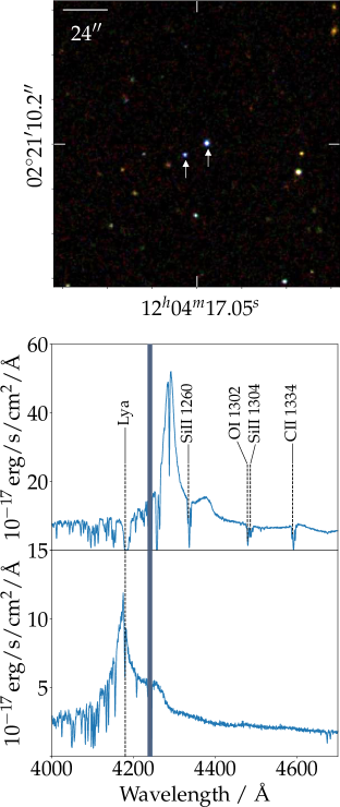
Figure 1: Illustrating the basic observation behind the QPQ experiment. The upper panel shows the projected quasar pair J1204+0221 at redshifts of z=$2.44$ and $z=2.53$. Photons from the background quasar pass through the halo of the foreground quasar and ionize HI and other atomic gas on their path. In the lower panel this process in manifested in the form of absorption line transitions in the spectrum of the background quasar (upper) at transition wavelengths corresponding to the redshift of the foreground quasar (lower). The shaded areas mask regions of bad data.

A major goal of the QPQ project has been to search for projected quasar pairs in optical spectroscopic and photometric surveys. The blue cutoff in the optical $u$ band falls at $\sim 3500$Å, which corresponds to the wavelength of the redshifted Ly$\alpha$ transition at $z\sim 2$. This is the limit at which one can reasonably detect atomic hydrogen at optical wavelengths and in large, ground-based surveys such as the SDSS. QPQ pair searches have therefore been focused towards pairs with foreground members within this redshift regime. Inevitably however, pairs outside of this redshift regime have found their way into the QPQ sample as false positives. These pairs are also included in the database, as are close physical binaries and gravitational lens candidates.

3 Quasar pair selection from spectroscopic surveys

A projected quasar pair is confirmed once spectra have been obtained that unambiguously reveal the spectral type of each pair member. In an age where spectroscopic redshift surveys have become a mainstay in extragalactic exploration, numbers of known quasar pairs have seen a corresponding spurt in growth.

Over the years, public spectroscopic survey projects have observed and cataloged over half a million quasars to redshifts in excess of $z=7$. Unquestionably, the largest compendium of quasar spectroscopy has been provided by the SDSS. Using straightforward spatial matching, QPQ has relied heavily on the annual spectroscopic data releases of the SDSS to select quasar pairs at separations of $\gtrsim$1^′. Due to fiber collisions, some pairs at closer separations require alternate techniques, which are discussed later in this section.

3.1 The SDSS Legacy Surveys

The original SDSS (York et al., 2000) ran between the years 2000-2008 and provides both imaging and spectroscopic coverage over $\sim 12,000\,\mathrm{deg^{2}}$ of the sky. The two components of the survey, SDSS-I and SDSS-II, ran consecutively on a dedicated 2.5 m telescope located at the Apache Point Observatory, in New Mexico (Gunn et al., 2006). Collectively, these surveys are now known as the SDSS Legacy survey (SDSS-LS).

SDSS-I ran during the first five years of operation and carried out multicolor $u\ (3551\,\text{\AA})$, $g\ (4686\,\text{\AA})$, $r\ (6166\,\text{\AA})$, $i\ (7480\,\text{\AA})$, $z\ (8932\,\text{\AA})$ (Fukugita et al., 1996; Stoughton et al., 2002; Doi et al., 2010) imaging and targeted spectroscopic follow-up within the imaging footprint. SDSS-II extended SDSS-I imaging footprint towards the Galactic plane.

The imaging and astrometric pipelines are described by Lupton et al. (2001) and Pier et al. (2003) respectively. Photometric calibration is tied to a standard star network (Hogg et al., 2001; Smith et al., 2002) and is refined to the $\sim 1$ per cent level via a global re-calibration (Padmanabhan et al., 2008). The $95\%$ completeness point source imaging depths are $u=22.0$, $g=22.2$, $r=22.2$, $i=21.3$ and $z=20.5$.

3.2 The SDSS Baryon Oscillation Spectroscopic Survey

The SDSS-LS was followed by SDSS-III, incorporating the Baryon Oscillation Spectroscopic Survey (BOSS; Dawson et al., 2013), which was designed to measure the scale of baryon acoustic oscillations (BAO) using quasars to trace the clustering of mass. SDSS-III extended the multi color imaging of the SDSS-LS by a further $\sim 2500\,\mathrm{deg}^{2}$ with the same telescope and camera between the years 2008-2009. All the SDSS imaging data was uniformly reduced with an improved sky subtraction and released under DR8 (Aihara et al., 2011), bringing the total imaging footprint to $14,555\,\mathrm{deg^{2}}$.

The remainder of the survey (2009-2014) was devoted to spectroscopy. The SDSS-LS spectrographs were upgraded (Smee et al., 2013) with new higher-efficiency volume holographic gratings, fully-depleted red CCDs with superior red response, blue CCDs with improved blue response and 1000 new fibers. Continuous wavelength coverage is provided between $3600$-$10,400\,\text{\AA}$ at resolutions between 1560-2270 in the blue channel and 1850-2650 in the red channel. Improved photometric selection algorithms were used to target 1.5 million luminous galaxies (Reid et al., 2016) and 150,000 new quasars in spectroscopy (Ross et al., 2012; Pâris et al., 2017).

3.3 The 2dF QSO Redshift Survey

Running in partial overlap with the SDSS surveys was the 2 degree Field (2dF) QSO Redshift Survey (2QZ; Croom et al., 2004). The QPQ search for quasar pairs in 2QZ was a similar search for spatially coincident catalog positions.

2QZ provides a homogeneous quasar catalog flux-limited to $16.00<b_{J}<20.85$. Candidates were color- selected via multi-wavelength $u$, $b_{J}$, $r$ photometry from automated plate measurement (APM) of UK Schmidt Telescope (UKST) photographic plates. These candidates were then observed by the 2dF instrument, a multi-object spectrograph at the Anglo-Australian Telescope (AAT). The 2QZ catalog comprises of 23,338 quasars spanning a redshift range of $0.3\lesssim z\lesssim 3.0$. The footprint covers a total area of $721.6\,\mathrm{deg}^{2}$ and is arranged over two contiguous strips of $75\degree\times 5\degree$ in area across the southern Galactic cap, centered on $\delta=-30\degree$ and northern Galactic cap centered on $\delta=0\degree$.

4 Quasar pair selection in imaging surveys

The 2QZ and SDSS surveys have made searching for quasar pairs a trivial endeavor with, however, the caveat that this method is inherently biased against close pairs due to the finite distance at which pairs of spectroscopic fibers can be placed from one another.

Approximately $30\%$ of the SDSS-LS and BOSS are covered spectroscopically in more than one epoch. These regions do not suffer from the effects of fiber collisions and close quasar pairs in these footprints can be drawn directly from the spectroscopic catalogs. Additionally, the 2QZ NGC region shares approximately half of its footprint with SDSS-LS, allowing 2QZ quasars to be assigned SDSS quasar pairs.

For the most part, however, fiber collisions prevent objects with separations of $<55\hbox{${}^{\prime\prime}$}$, $<62\hbox{${}^{\prime\prime}$}$ and $<30\hbox{${}^{\prime\prime}$}$ from being observed simultaneously in SDSS-LS, BOSS and 2QZ respectively (Blanton et al., 2003; Dawson et al., 2013; Lewis et al., 2002). Therefore in most cases, close quasar pairs are selected by spatially matching to photometrically targeted objects with quasar-like colors in close proximity to spectroscopically cataloged quasars. Photometric candidates are later followed-up spectroscopically to confirm the pair.

QPQ has used SDSS imaging to select photometric quasar pair members in this way via three distinct methods. Hennawi et al. (2006a) described a means to select pairs at similar redshifts via a $\chi^{2}$ selection statistic, which utilizes the fact that the rest-frame UV to optical spectral energy distributions of quasars follow a remarkably tight color redshift relation. If one neglects the relatively small intrinsic scatter of the population about this relation, then the fluxes of a pair of quasars at the same redshift should be related by a single proportionality constant across all bands. Variation in this proportionality can then be approximately attributed to observational error. One can find the constant of proportionality that minimizes the sum of the differences in flux between pairs across all bands. In this way it is possible to efficiently select close pairs of quasars at similar redshifts.

To select close quasar pairs at differing redshifts, Hennawi et al. (2006a) (see also Myers et al., 2007, 2008; Eftekharzadeh et al., 2017) made use of the various photometric catalogs collated by Richards et al. (2004, 2009a, 2009b, 2015). Richards et. al. used kernel density estimation to model the probability density functions of stars and quasars in the 4-D SDSS color space. The likelihood that a given photometric object originates from either of these two distributions is combined with prior knowledge of quasar and stellar number densities using Bayes’ theorem. The result is a probabilistic classification of an object as either a star or a quasar. QPQ mined these catalogs for both photometric-photometric and photometric-spectroscopic pairs with large quasar probabilities. Candidates were then followed up spectroscopically.

Bovy et al. (2011) compiled a targeting catalog of photometric quasar candidates for BOSS using a non-parametric Bayesian classifier that represents an advance on the Richards et al. technique by approximating the underlying density distributions of stars and galaxies in flux space via an extreme-deconvolution. The classification code, XDQSO, was extended to provide probabilistic selection over arbitrary redshift intervals as well as incorporating UV and near- infrared (IR) information (XDQSOz; Bovy et al., 2012). Further details of the continuing effort to discover both photometric-spectroscopic and photometric-photometric quasar pairs is detailed in Hennawi (2004) and Hennawi et al. (2006a, 2010).

5 New pairs from SDSS, ATLAS & WISE

The most recent QPQ search for photometric-photometric pairs was conducted in optical imaging from the SDSS and VST ATLAS (Shanks et al., 2015) surveys combined with mid-IR data from the Wide- Field Infrared Survey Explorer (WISE; Wright et al., 2010). Unlike the searches described in previous sections, this search has not been discussed in any previous publication, it is described here in detail for the first time.

5.1 The VST ATLAS Survey

ATLAS is an optical $u$, $g$, $r$, $i$, $z$ survey carried out by OmegaCam (Kuijken, 2011) on the European Southern Observatory’s (ESO) $2.61\,\mathrm{m}$ VLT Survey Telescope (VST; Schipani et al., 2012) at the Cerro Paranal Observatory in Chile. ATLAS has completed its final $4711\,\mathrm{deg}^{2}$ footprint in all filters over two contiguous regions covering the northern and southern Galactic caps during 6 years of observations. The premise of the ATLAS survey is to provide imaging in the southern hemisphere with equivalent depth and better image quality than SDSS.

The ATLAS data is reduced by end-to-end astrometric and photometric pipelines run by the Cambridge Astronomical Survey Unit (CASU) and archived by the Wide Field Astronomy Unit (WFAU) in the OmegaCam Science Archive (OSA).

5.2 The Wide-Field Infrared Survey Explorer

WISE was launched in December 2009 and from February to August 2010, surveyed the entire sky in four mid-IR bands W1 ($3.4\,\mu\mathrm{m}$), W2 ($4.6\,\mu\mathrm{m}$), W3 ($12\,\mu\mathrm{m}$) and W4  ($22\,\mu\mathrm{m}$). This initial survey release, termed the "AllSky" release, represents a significant step forward in exploration of the mid-IR sky at these wavelengths. The 5$\sigma$ AB point source sensitivity limits are deeper than 19.1, 18.8, 16.4 and 14.5 mag in W1-W4 respectively, providing over a hundred times the sensitivity of the $12\mu\mathrm{m}$ band of the InfraRed Astronomical satellite (IRAS; Neugebauer et al., 1984).

In September 2010 the cryogen cooling the W3 and W4 instruments depleted, ending the full four band mission. The W1 and W2 band missions continued through February 2011 encompassing both the AllWISE and Near Earth Object WISE (NEOWISE; Mainzer et al., 2011) data releases. After a period of hibernation this was followed by the NEOWISE Reactivation mission (NEOWISER; Mainzer et al., 2014) in October 2013, which is still in operation at the time of writing (March 2018).

5.3 Data preparation & candidate selection

SDSS and ATLAS differ widely to WISE in depth, resolution and wavelength and as a result there are significant benefits to forced photometry in WISE images at optical positions compared to traditional positional catalog matching. The angular resolution of the WISE imaging is diffraction-limited and at long mid-IR wavelengths this translates into a resolving power of several arcseconds. Conversely, the angular resolution of the optical imaging catalogs are seeing limited, translating to roughly 1.0^′′ at the median. Forced photometry ensures that the optical and WISE measurements are linked to a consistent set of sources, whereas catalog-matching would inevitably lead to a tail of wide separation erroneous positional matches.

Furthermore the bulk of SDSS and ATLAS quasar candidates lie towards the limiting depths of the respective catalogs. Many of these sources are undetected at the shallower limiting depths of the AllWISE public release catalogs. Measurements of these faint or even undetected sources in WISE are just as scientifically valuable as a significant detection, particularly for the sophisticated statistical selection techniques described in section 4.

The full-depth coadded WISE images are available as part of the AllWISE data release. These full-depth images are convolved by the point spread function (PSF) during the coaddition process. This step is included to improve the detection of isolated point sources but it is inappropriate for other applications such as forced photometry, since the blurring of the PSF decreases the available signal-to-noise. Lang (2014) provide an independent reduction of the AllWISE data products, which consists of full-depth coadds at the full instrument resolution. These data products, termed the “unWISE” coadds, were used to assemble a catalog of mid-IR photometry forced at the sites of over 400 million SDSS sources (Lang et al., 2016). Closely following this release, the XDQSOz selection code was updated to incorporate the unWISE imaging and a catalog of over 5 million photometric quasar candidates was generated over the SDSS footprint (DiPompeo et al., 2015). This candidate list served as the starting point for the photometric pair search in SDSS and WISE.

More recently Meisner et al. (2017) have undertaken further reprocessing of AllWISE, incorporating three years of NEOWISER imaging into the unWISE framework. The coadded data products provide significant gains in depth over the original unWISE release and, in addition, time dependent artifacts such as moon contamination are largely eliminated because of the inclusion of multiple epochs.

Band merged ATLAS source catalogs provided by CASU were force photometered at the W1 and W2 bandpasses in the unWISE coadds of Meisner et al. (2017). The forced photometry was performed by the Tractor (Lang et al. in preparation). The Tractor is an innovative code for inference modeling of astronomical sources. The premise is the optimization of a likelihood for the source properties given a set of imaging data and an informative noise model. The details of the Tractor implementation running in forced photometry mode on the unWISE coadds is discussed by Lang et al. (2016). The QPQ Tractor run follows this closely.

QPQ used the updated XDQSOz selection code to construct a catalog of quasar candidates from ATLAS and forced unWISE imaging over a fraction of the ATLAS footprint. This catalog, along with the SDSS-unWISE catalog described above were then mined for close pairs of objects with $>90\%$ quasar probabilities. Candidates were selected to $r<22$ but emphasis was typically placed on selecting pairs with $r<21$ and with foreground members at $z>3$. All pairs within 1^′ were considered for follow up, but priority was given to pairs within $<30$^′′.

The benefits of combining WISE mid-IR data into the established $ugriz$ optical quasar selection method has been explored since the WISE AllSky data release in March 2012 (e.g. Wu et al., 2012). Among the first projects to explore this practically were the SDSS-IV Extended Baryon Oscillation Spectroscopic Survey (eBOSS; Myers et al., 2015) and the 2dF Quasar Dark Energy Survey pilot (2QDESp; Chehade et al., 2016), a spectroscopic survey of quasar candidates selected in ATLAS and WISE imaging. These projects showed the utility of the infrared excess in quasar SEDs to achieve large separations between the quasar and stellar loci. The utility of the WISE mid-IR imaging can be seen in Figure 2, where the quasar pair database is plotted along side stars for four different color-color combinations including the SDSS and WISE W1 passbands. Only where WISE data is incorporated, as in the lower right-hand panel, is there a significant distinction between the stellar and quasar loci.

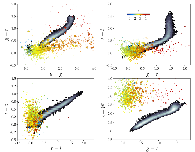
Figure 2: Color-color plots showing the stellar locus in gray scale and the quasar pair database color coded according to redshift. The benefit of introducing the WISE W1 band to SDSS $ugriz$ color combinations is seen in the bottom right hand panel, where quasars and stars occupy distinct regions of color-color space. The star shaped symbols show quasar pairs discovered during the recent QPQ search in ATLAS, SDSS and WISE imaging. The circles show the remainder to the QPQ pair database. No attempt has been made here to place the ATLAS photometry on to the SDSS system; at the scales presented here the differences are completely negligible.

5.4 Spectroscopic follow up

Candidates at declination $>-20~{}\rm deg$ (all those presented here) were observed on the Intermediate dispersion Spectrograph and Imaging System (ISIS; Jorden, 1990), mounted at the Cassegrain focus of the 4.2 m William Herschel Telescope (WHT). The observing run was conducted on 22 nights between December 2015 and March 2016 as part of program 2015/P1 and 2016/P6. Approximately three nights were lost due to poor weather. Usable nights were for the most part clear but not always photometric.

The instrument was configured with R300B and R316R gratings centered at 4230 Å and 6400 Å in the blue and red arms respectively, with the D5300 dichroic filter in place over both channels. A 1^′′slit width combined with a factor 2 binning in the dispersion direction at readout time, resulted in continuous wavelength coverage over $3000-7630$ Å with average resolutions of $R\sim 4.1$Å and $R\sim 3.8$Å in the blue and red channels respectively.

The data were reduced using the Low-Redux pipeline extended to work with the ISIS detectors. This pipeline performs basic calibrations (bias, flat-fielding, and wavelength calibration), and extracts flux-calibrated 1D spectra which are then coadded across multiple exposures. All spectra were visually inspected to separate stars from quasars, and to measure the quasar redshifts by superposing a quasar template to the data.

In total, 69 photometrically selected pairs in ATLAS were observed on WHT, resulting in 15 new projected quasar pairs. The remaining observing time was devoted to observations of candidates selected from SDSS, yielding the discovery of 39 new pairs.

The foreground quasars are distributed between $z\approx 0.8$-$3.6$ and their halos are probed by their background counterparts over physical scales of $\mathrm{R_{\perp}}\approx 0.1$-$0.5\,\mathrm{Mpc}$. The coordinates, redshifts, on-sky and physical separations are given for the new quasar pairs in Table 1. The star symbols in Figure 2 show the positions of the new projected quasars in $ugrizW1$ color-color space and are color coded according to their redshifts.

Table 1: Table of new quasar pairs discovered in combined ATLAS, SDSS and WISE imaging.

$\mathrm{QSO_{fg}}$	$\mathrm{QSO_{bg}}$	$z_{\mathrm{fg}}$	$z_{\mathrm{bg}}$	$\theta\hbox{${}^{\prime}$}$	$R_{\perp}\ (\mathrm{pkpc})$	Survey
J003308.63-083222.19	J003307.31-083241.55	3.038	3.043	0.459	216.433	SDSS
J012902.78+191824.46	J012901.92+191847.18	2.680	2.691	0.430	209.778	SDSS
J015415.22+032455.84	J015416.43+032457.86	2.660	3.219	0.304	148.640	SDSS
J022845.72-124643.92	J022848.07-124706.78	1.733	2.032	0.688	358.303	ATLAS
J023229.05-100123.48	J023231.25-100102.92	2.063	2.386	0.641	328.856	ATLAS
J031855.31-103040.30	J031853.87-102945.32	2.226	2.417	0.982	498.485	ATLAS
J032926.40-134732.22	J032926.04-134831.51	2.073	2.372	0.992	508.701	ATLAS
J033347.40-133928.44	J033345.40-133938.41	2.230	2.679	0.513	260.495	ATLAS
J034952.34-110620.59	J034955.77-110642.91	2.449	2.824	0.920	458.622	ATLAS
J090551.96+253003.35	J090551.25+253026.09	3.325	3.300	0.411	188.462	SDSS
J090828.30+080313.18	J090826.82+080320.34	2.390	3.168	0.385	193.025	SDSS
J091800.77+153621.46	J091800.70+153631.31	2.980	2.958	0.165	78.282	SDSS
J093240.91+400905.65	J093243.02+400913.95	2.962	3.130	0.426	202.556	SDSS
J093836.78+100905.34	J093837.81+100922.00	2.504	2.818	0.376	186.529	SDSS
J095503.57+614242.66	J095503.14+614247.33	2.739	2.725	0.093	45.173	SDSS
J095549.38+153838.11	J095549.80+153837.00	0.830	2.900	0.103	48.214	SDSS
J095629.72+243441.34	J095627.88+243436.98	2.979	2.914	0.425	201.423	SDSS
J100205.70+462411.82	J100202.89+462407.25	3.138	2.760	0.490	228.948	SDSS
J100253.37+341924.03	J100254.22+341928.47	2.418	2.506	0.190	95.194	SDSS
J100903.16-142104.27	J100859.11-142114.19	2.033	2.068	0.995	511.335	ATLAS
J101853.24-160727.80	J101853.10-160808.04	2.331	2.953	0.672	338.026	ATLAS
J102947.32+120817.11	J102945.77+120824.53	2.820	3.392	0.399	192.024	SDSS
J103109.37+375749.68	J103108.25+375801.19	2.752	2.589	0.292	141.842	SDSS
J103716.68+430915.57	J103716.86+430944.83	2.676	3.286	0.489	238.758	SDSS
J104314.33+143434.81	J104313.69+143435.73	2.980	3.361	0.156	73.812	SDSS
J104339.12+010531.29	J104338.28+010507.77	3.240	3.001	0.445	205.465	SDSS
J105202.95-103803.70	J105203.23-103815.09	2.104	2.194	0.202	103.336	ATLAS
J105338.15-081623.66	J105336.09-081620.94	2.192	2.294	0.512	260.282	ATLAS
J105354.90-100941.44	J105354.48-100931.71	3.232	3.248	0.192	88.924	ATLAS
J110402.08+132154.46	J110401.42+132134.70	2.869	2.576	0.366	175.702	SDSS
J110124.79-105645.12	J110126.03-105642.26	2.579	2.688	0.308	151.832	ATLAS
J111820.36+044120.22	J111820.46+044125.26	3.120	3.454	0.088	40.981	SDSS
J112032.04-095203.21	J112032.65-095138.28	2.180	3.627	0.442	224.954	ATLAS
J112239.32+450618.54	J112236.72+450628.12	3.590	3.044	0.486	216.459	SDSS
J112355.97-125040.73	J112359.53-125056.76	2.965	3.428	0.908	431.314	ATLAS
J112516.06+284057.59	J112516.26+284122.74	2.845	2.834	0.421	202.590	SDSS
J112839.64-144842.36	J112843.30-144837.44	1.920	2.200	0.888	459.457	ATLAS
J112913.52+662039.13	J112915.28+662101.63	2.807	2.803	0.414	199.966	SDSS
J113820.28+203336.93	J113820.42+203333.18	2.687	2.679	0.071	34.437	SDSS
J114443.59+102143.48	J114442.32+102125.21	1.503	2.833	0.436	227.342	SDSS
J115037.52+422421.01	J115035.53+422409.90	2.883	3.126	0.411	197.017	SDSS
J115222.15+271543.29	J115221.84+271540.80	3.102	3.083	0.080	37.686	SDSS
J120032.34+491951.99	J120034.26+492015.22	2.629	3.254	0.498	244.193	SDSS
J121642.25+292537.97	J121641.77+292529.34	2.532	2.519	0.178	87.996	SDSS
J122900.87+422243.23	J122859.36+422229.73	3.842	3.459	0.358	155.535	SDSS
J123055.78+184746.79	J123056.94+184736.83	3.169	3.089	0.321	149.312	SDSS
J132728.77+271311.96	J132729.83+271324.94	3.085	2.658	0.320	150.152	SDSS
J134221.26+215041.97	J134219.85+215051.20	3.062	2.506	0.362	170.098	SDSS
J135456.96+494143.74	J135456.76+494154.08	3.126	2.928	0.175	81.962	SDSS
J141457.24+242039.67	J141457.12+242106.23	3.576	3.515	0.444	197.922	SDSS
J143622.50+424127.13	J143622.01+424132.22	3.000	3.050	0.124	58.564	SDSS
J144225.30+625600.96	J144223.04+625625.99	3.271	3.271	0.490	225.685	SDSS
J162413.70+183330.72	J162412.59+183348.25	2.763	3.263	0.393	190.480	SDSS
J214858.11-074033.28	J214858.06-074034.98	2.660	2.660	0.031	15.128	SDSS

Note. — From left to right columns give the names of the foreground and background quasars, the foreground and background quasar redshifts, the on-sky angular separation between the pair in arcminutes, the physical transverse distance between the line of sight of the background quasar and the foreground quasar in pkpc and the survey in which the pair was discovered.

6 The Quasar pair database

The database of quasar pairs comprises a catalog and a spectral library both housed within a single HDF5 specDB file. specDB is a software package for generating and interfacing with databases of astronomical spectra, written and maintained by JXP. The following sections focus on the database content, source and data characteristics and the database architecture. Full documentation of the specDB package, including download instructions for the spectral database, are supplied by Read the Docs. We further note that the igmspec database, also under specDB, provides approximately 500,000 quasar spectra from public and private datasets (Prochaska, 2017). In keeping with its goals, which include maintaining a highly complete database of quasar spectra in a consistent format, the quasar pair spectra will also be ingested into igmspec, however some of the catalog content will only be available via the QPQ pair catalog presented here.

6.1 The catalog

The quasar pair catalog comprises of a simple table containing a single record for each unique source. Distinct catalog records are uniquely identified via a primary key. The catalog also contains celestial coordinates, redshifts, references to the aforementioned, a redshift uncertainty column, which remains empty and UV and mid-IR photometry for all pairs within $5\hbox{${}^{\prime}$}$ of separation. The celestial coordinates come largely from PanStarrs (Chambers et al., 2016) because, except for a small fraction of objects that fall outside of the footprint, PanStarrs covers the entire catalog with sub-arcsecond accuracy.

The catalog redshifts are estimated via a wide range of distinct methodologies from a variety of sources including cross correlation (Hewett & Wild, 2010), principle component analysis (Pâris et al., 2012), spectral line fitting (QPQ6) and visual inspection (this submission). The most significant difficulty in estimating quasar redshifts is in accounting for the natural variance in emission line properties of the quasar population both as a function of redshift and luminosity. This variation is large and ill-understood and some redshift estimators are better than others in accounting for it. Consolidating redshift uncertainties with differing systematics into a single table would be inconsistent and misleading. Instead redshift uncertainties have been estimated at $\delta\simeq\,1000\mathrm{km\,s^{-1}}$, which is conservative. The redshift uncertainty column is empty but remains in the catalog to facilitate future attempts to measure redshifts more consistently (see section  7).

Columns of mid-IR and UV photometry are provided via measurements made at the positions of catalog objects in the unWISE coadds (section 5) and the Galaxy Evolution Explorer (GALEX; Morrissey et al., 2007) imaging products. Forced photometry from these two surveys is included for the reasons discussed in section 5.

GALEX undertook wide field surveys in both imaging and low resolution grism spectroscopy from May 2003 until February 2012. It delivered the first broadband imaging surveys in the far-UV and near-UV at central wavelengths of $1528$Å and $2310$Å respectively.

Flux-calibrated, background-subtracted intensity maps as well as the sky background and threshold weight maps are served by the Barbara A. Mikulski Archive for Space Telescopes (MAST). The GALEX photometry pipeline (Morrissey et al., 2007) passes these products through SExtractor (Bertin & Arnouts, 1996) to obtain calibrated catalogs. MAST also serves the SExtractor configuration and parameter files necessary for computing photometery on each individual image. In principle then, one should be able to reconstruct any GALEX catalog in the official release. The slight complication with forced photometry is the need to bypass the source detection stage and simply place apertures down at predefined pixel positions. SExtractor does not have this facility and therefore forced photometry was performed by constructing mock images with mock sources at the position of the object of interest. SExtractor was then run in dual image mode, which allows the mock image to be used for the purposes of source detection and the real image to be used for the source extraction, thereby extracting the real source from the real image at the position of the mock source in the mock image. Beyond this modification the procedure follows that of the actual GALEX photometry pipeline. Photometry is provided for a 6^′′ radius aperture, which is a reasonable compromise between minimizing background noise contributions and measuring photometry towards the field edges where the PSF becomes degraded.

The results of the unWISE and GALEX forced photometry are verified in Figures 3 and 4 respectively, where members of the quasar pair catalog which are detected in the officially released AllWISE or GALEX catalogs are plotted against the forced photometry. In Figure 3 the left-hand panels show the comparison of AllWISE and unWISE photometry and the orange lines show a one-to-one relationship. The plot axes extend to the average $3\sigma$ depth of the official release in each band and the dashed lines show the average $5\sigma$ depth in each band. The right-hand panels compare magnitude errors. The benefits of using the unWISE products over the official AllWISE release are clear. Significant gains in signal-noise are achieved in all bands and particularly in W1 and W2 where the addition of the NEOWISE observations have almost doubled the signal-noise over the AllWISE release.

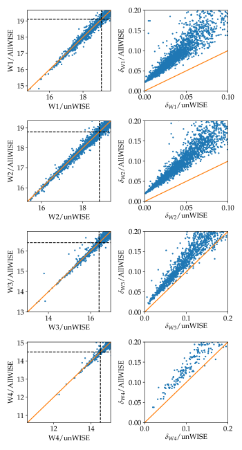
Figure 3: A comparison of the AllWISE photometry of detected quasar pairs with the forced photometry of the unWISE images. Left had panels show the magnitude measurements from the AllWISE release versus the forced measurements. The orange line shows a one-to-one relationship and the dashed lines are placed at the average $5\sigma$ AllWISE limiting magnitudes. The right hand panels compare the magnitude errors. The gains in the unWISE over the AllWISE dataset are obviously apparent, especially in the W1 and W2 bands where the addition of NEOWISE and NEOWISER data has approximately doubled the signal-noise.

Figure 4 shows a similar comparison between the officially released and forced GALEX photometry. The forced photometry in both cases, unWISE and GALEX, is in good agreement with their respective official releases. Forced photometry of quasar pairs in optical or near-IR surveys is omitted from the catalog since straight-forward catalog matching is both efficient and accurate at the fine spatial resolutions offered by modern surveys in these wavelength regimes.

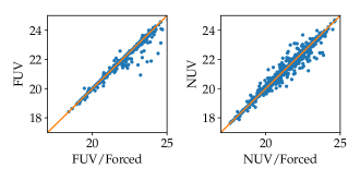
Figure 4: A comparison of officially released GALEX photometry for detected quasars versus forced photometry. The left panel shows FUV photometry and the right panel shows NUV photometry. The orange line shows a one-to-one relationship and the two sets of measurements are in good agreement, which serves to verify the forced photometry method.

A full description of the catalog is given in Table 3. Figure 5 shows the sky coverage of the catalog with points plotted at the locations of all foreground quasars and color coded according to redshift. The filled regions correspond to the imaging footprints of the surveys that bound the QPQ quasar searches, namely SDSS-LS, BOSS, ATLAS and 2QZ. The background map shows the Milky Way polarized dust emission from the Planck commander component separation (Planck Collaboration et al., 2015).

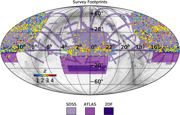
Figure 5: The sky coverage of the QPQ catalog in equatorial coordinates. Points show the locations of all foreground quasar pair members and are color coded according to redshift. The shaded regions show the various survey footprints which bound the QPQ search area and are color coded as given in the legend. The SDSS-LS and BOSS imaging footprints are plotted in the same color labeled “SDSS". The gray scale background shows the Milky Way polarized dust emission as seen by Planck.

The distribution of foreground quasar redshifts is shown in the right hand panel of the joint-plot in Figure 6. The distribution peaks at $z\sim 2.5$, corresponding to the peak in cosmic quasar activity. From the redshifts of foreground and background pair members and the known angular separations between them, one can compute the proper transverse separation of a foreground quasar to the sightline of the background quasar. The distribution of proper transverse separations is shown in the upper panel of Figure 6 and the joint distribution with redshift is shown in the main panel of the same Figure. Physical binaries are omitted in each of these plots by cutting the sample to pairs with velocity differences of $>3000\,\mathrm{km\,s^{-1}}$. This plot serves to illustrate the range of environments probed by the background quasar sightlines. Distances of tens of $\mathrm{pkpc}$, corresponding to the outer regions of galactic discs to hundreds of $\mathrm{pkpc}$, probing the CGM, to a few $\mathrm{pMpc}$ corresponding to scales in the cosmic web are all probed by the background sources.

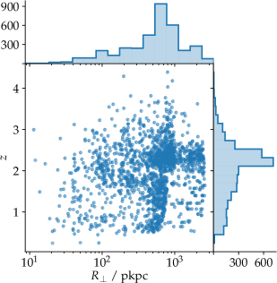
Figure 6: The joint distribution of redshift and physical transverse separation $R_{\perp}$ is shown in the main panel. Each is also plotted independently in the histograms on the peripheral panels. The peak in the redshift distribution corresponds to the peak in cosmic AGN activity. The distribution of physical transverse separation shows that the catalog probes the halos of quasars at impact parameters of tens of physical kpc to a few Mpc. Physical binaries are omitted in each of these plots by cutting the sample to pairs with velocity differences of $>3000\,\mathrm{km\,s^{-1}}$.

6.2 The spectroscopic library

The spectroscopic library houses the spectra of quasar pairs in the catalog listing. There may be multiple spectra associated with any distinct catalog source. The spectroscopic library is a heterogeneous data set which includes low to moderate to high resolution spectra with wavelength coverage from the optical to the near-IR. The low and many of the moderate resolution spectra generally result from QPQ campaigns focused on fast and efficient spectroscopic identification of photometric targets. A significant fraction of the optical, moderate-resolution spectra come from SDSS-LS or BOSS. The high resolution spectra were specifically targeted towards and have been used in detailed studies of the CGM (; ).

Over the years, related projects with broadened science goals have extended the QPQ catalog further. The various science cases have included measuring the small-scale clustering of quasars (Hennawi et al., 2006a; Myers et al., 2007, 2008; Hennawi et al., 2010; Shen et al., 2010; Eftekharzadeh et al., 2017), exploring correlations in the IGM along close separation sightlines (Ellison et al., 2007; Martin et al., 2010), analyzing small-scale transverse Ly$\alpha$ forest correlations (Rorai et al., 2013), characterizing the transverse proximity effect (Schmidt et al., 2017), probing the halos of damped Ly$\alpha$ systems (DLAs; Rubin et al., 2015)and correcting CIV-based virial BH masses (Coatman et al., 2017)

The latter submission describes the near-infrared spectra of approximately 120 quasar pairs observed as part of QPQ follow-up programs. Coatman et al. also provide an additional  500 near-IR quasar spectra of non-pairs compiled both from the literature and from their own observations. At the time of writing all the Coatman et al. near-IR spectra are restricted to proprietary use but are expected to become publicly available in the very near future . As soon as this occurs, the near-IR pair spectra will be ingested by the QPQ database.

The range in resolving power covered by the spectral library is shown for each instrument in Figure 7. The wavelength coverage of the spectra are characterized in Table 2, with respect to the optical and near-IR broad-band filters of the SDSS and UKIDSS imaging surveys. Each row corresponds to a particular telescope and instrument in the catalog. Column “Total” refers to the total number of spectra. The columns $ugriz$YJHK refer to the SDSS or UKIDSS passbands of the same name and indicate the number of spectra with coverage in those passpands. A spectrum is arbitrarily considered to have coverage in a given passband when its wavelength array falls entirely or partially within the cut-on and cut-off wavelengths at 50 percent transmission. To avoid counting the less useful low signal-noise regions of any spectrum (usually found towards detector edges), positive wavelength coverage also requires that the average signal-noise in the 50 pixels either side of the central covering pixel is at least 3.

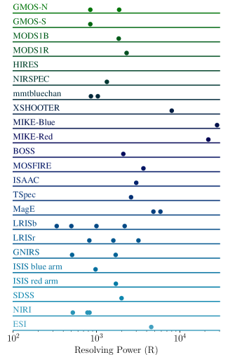
Figure 7: The range in spectral resolving power grouped by instrument. Resolving power (R) is given along the $x$-axis for each instrument listed on the $y$-axis. Note that no numerical scale is associated with the $y$-axis and that this figure does not give information pertaining to the number of spectra associated with a given instrument (see Table 2). Rather unique R-values for all spectra associated with a given instrument are represented by single points along the $x$-axis.

Table 2: Wavelength coverage

Telescope	Instrument	Total	$u$	$g$	$r$	$i$	$z$	$Y$	$J$	$H$	$K$
Gemini-North	GMOS-N	71	28	70	37	0	0	0	0	0	0
Gemini-North	NIRI	33	0	0	0	0	0	0	0	30	3
Gemini-South	GMOS-S	36	3	34	36	6	0	0	0	0	0
Gemini-South	GNIRS	29	0	0	0	2	24	28	29	28	29
MGIO-LBT	MODS1B	10	7	10	0	0	0	0	0	0	0
MGIO-LBT	MODS1R	10	0	0	10	10	10	0	0	0	0
Keck-I	LRISb	358	258	216	129	0	0	0	0	0	0
Keck-I	LRISr	140	0	0	136	136	134	0	0	0	0
Keck-I	HIRES	1	1	1	1	0	0	0	0	0	0
Keck-I	MOSFIRE	2	0	0	0	0	0	0	1	2	0
Keck-II	NIRSPEC	5	0	0	0	0	0	0	0	2	2
Keck-II	ESI	115	0	86	109	112	108	89	0	0	0
MMTO	mmtbluechan	91	68	87	22	0	0	0	0	0	0
ESO-VLT-U2	XSHOOTER	36	15	32	33	32	29	23	33	34	8
ESO-VLT-U3	ISAAC	17	0	0	0	0	0	0	0	17	0
Clay (Mag.II)	MIKE-Blue	6	2	5	2	2	2	0	0	0	0
Clay (Mag.II)	MIKE-Red	4	0	4	4	4	2	0	0	0	0
Clay_Mag_2	MagE	76	32	73	75	75	74	39	0	0	0
SDSS 2.5-M	SDSS	88	46	72	83	83	57	0	0	0	0
SDSS 2.5-M	BOSS	2304	526	1896	1539	1526	1305	221	0	0	0
200	TSpec	68	0	0	0	0	0	64	67	67	52
WHT	ISIS blue arm	41	0	23	0	0	0	0	0	0	0
WHT	ISIS red arm	41	0	0	35	29	0	0	0	0	0

Note. — Wavelength coverage of individual spectra in the spectral library. Wavelength coverage is described with respect to the $ugrizYJHK$ bandpasses of the SDSS and UKIDSS imaging surveys. A spectrum is arbitrarily defined to have coverage in a particular bandpass if its wavelength array falls within the interval of the cut-on cut-off values at 50 per cent of the peak bandpass transmission. In order to avoid counting low signal-noise regions of the spectrum, the average signal-noise in the 50 pixels either side of the central covering pixel must have signal-noise of at least 3. The column “Total” gives the total number of spectra grouped according to a particular Telescope and instrument combination. The columns $ugrizYJHK$ give the number of spectra deemed to have coverage in that bandpass.

6.3 Database Architecture

The database comprises a catalog listing and a spectral library. The catalog listing is a simple table containing one record for each unique source in the database. Each field in the catalog is described in Table 3. The spectral library may contain one or more spectra for each individual catalog source. A catalog record is linked to its corresponding spectra via a primary key field unique at the catalog level and having a one to many relationship with all spectra associated to that source.

Table 3: Catalog schema.

Key	Type	Depscription
QPQ_ID	INT	Primary key unique identifier
flag_group	INT	Bitwise flag indicating the groups that the source has spectra in
zem	FLOAT	Emission redshift of source
sig_zem	FLOAT	Estimated error in the redshift
flag_zem	STR	Key indicating source of the redshift
RA	FLOAT	Celestial Right Ascension in decimal degrees
DEC	FLOAT	Celestial declination in decimal degrees
flag_coo	STR	Key indicating source of the coordinates
STYPE	STR	Spectral type (e.g. QSO)
W1_FLUX	FLOAT	WISE W1 AB flux in nanomaggies
W2_FLUX	FLOAT	WISE W2 AB flux in nanomaggies
W3_FLUX	FLOAT	WISE W3 AB flux in nanomaggies
W4_FLUX	FLOAT	WISE W4 AB flux in nanomaggies
W1_IVAR	FLOAT	WISE W1 AB invserse variance in nanomagies-2
W2_IVAR	FLOAT	WISE W2 AB invserse variance in nanomaggies-2
W3_IVAR	FLOAT	WISE W3 AB invserse variance in nanomaggies-2
W4_IVAR	FLOAT	WISE W4 AB invserse variance in nanomaggies-2
FUV_FLUX	FLOAT	GALEX FUV AB flux in nanomaggies
NUV_FLUX	FLOAT	GALEX NUV AB flux in nanomaggies
FUV_IVAR	FLOAT	GALEX FUV AB invserse variance in nanomaggies-2
NUV_IVAR	FLOAT	GALEX NUV AB invserse variance in nanomaggies-2

Within the spectral library, spectra are arranged within a set of distinct groups. Each group contains the spectra and a meta-data table, which maintains a list of the common properties pertaining to each spectrum, including the primary key, wavelength coverage, resolving power, telescope and instrument etc. Entries in the meta-data table are ordered identically and aligned row-by-row with their corresponding spectra. A complete description of the meta-data fields is given in Table 4.

Table 4: Meta-data schema.

Key	Type	Depscription
QPQ_ID	INT	Primary key unique at the catalog level
GROUP_ID	INT	Primary key unique at the group level
IGM_ID	INT	Primary key reference in to igmspec
zem_GROUP	FLOAT	Emission redshift
sig_zem	FLOAT	Estimated error in the redshift
flag_zem	STR	Key indicating source of the redshift
RA_GROUP	FLOAT	Right Ascension in decimal degrees
DEC_GROUP	FLOAT	Declination in decimal degrees
EPOCH	FLOAT	Year of epoch
R	FLOAT	Spectral resolution ($\delta\lambda/\lambda$): FWHM
WV_MIN	FLOAT	Minimum wavelength value in Å
WV_MAX	FLOAT	Maximum wavelength value in Å
NPIX	INT	Number of pixels in the spectrum
SPEC_FILE	STR	Individual filename of the spectrum
STYPE	STR	Spectral type (e.g. QSO)
INSTR	STR	Instrument
DISPERSER	STR	Dispersing element
TELESCOPE	STR	Name of the telescope
GROUP	STR	Name of group
DATE-OBS	STR	Observation date

The groups themselves are assigned and named according to the spectrograph used to measure the spectrum. A list of the groups can be found in Table 5. Note that in most cases the name of the group is identical to the corresponding value in the instrument meta-data field. However, there are a few instances where this is not the case. In particular where a set of observations on a single spectrograph result in a blue channel and a red channel spectrum and these spectra have not been merged, then two instruments exist inside a single group, one for the red channel and one for the blue channel.

Table 5: Groups within the spectral library.

Group Names
GMOS	ISAAC	MODS
TRIPLESPEC	HIRES	MAGE
NIRSPEC	LRIS	MMT
GNIRS	XSHOOTER	SDSS
MIKE	NIRI	BOSS
ESI	MOSFIRE	ISIS

Given this simple architecture it is straightforward to pull spectra out of the library given a catalog search. For example one may query the catalog on any number of its fields to obtain a subsidiary table built to the query constraints. The primary key field of the subsidiary table can then be used to query the spectral library and retrieve the desired spectra. Of course, the catalog, spectral library and meta-data can also be queried independently of one another.

7 Summary & Future Work

With the addition here of 54 newly discovered quasar pairs from VST ATLAS, SDSS and WISE, the QPQ database contains catalog listings for over 5500 distinct objects and a spectral database containing over 3500 optical and near-infrared spectra of projected quasar pairs, quasars closely separated in redshift and gravitational lens candidates. The database is the fruit of over a decade of work, nine previously published articles and many other related projects and studies. The projected pairs provide a means to probe the $z>2$ CGM of quasar host galaxies at impact parameters of tens of $\mathrm{pkpc}$ through to several $\mathrm{pMpc}$ or equivalently from scales comparable in extent to galactic discs, to bound gas in the CGM and to nearby regions of intergalactic space. In publishing this catalog the hope is to provide a laboratory for future discoveries in the CGM of massive galaxies hosting quasars. This database serves as a living resource which will continue to grow, reflecting advances in both scientific understanding and instrumentation.

New multi-fiber spectrographs such as DESI (Dark Energy Spectroscopic Instrument; DESI Collaboration et al., 2016) and Suburu PSF (Prime Focus Spectrograph; Tamura et al., 2016) will supply the data sets for future catalog expansion. DESI alone will target and obtain redshifts for over $\sim 700,000$ quasars at $z\gtrsim 2$, providing gains of over 3 times in comparison to the combined SDSS, BOSS and the ongoing eBOSS quasar redshift surveys. The QPQ project lays the foundation for future pair searches in these data sets as well as the techniques to be able to study them in unprecedented and exquisite statistical detail.

The promise of future large spectroscopic surveys demands increasing numbers of parallel, detailed case studies. To that end, the pursuit of a much larger sample of high-resolution, high signal-noise spectra is of prime importance. The complexities of the CGM are manifest in its rich multiphase, multiscale structures, which display distinct kinematics and metallicities. The detailed dissection of all facets of the CGM requires the capability to resolve its smallest coherent structures. With current ground-based 10 m telescopes few QPQ pairs are currently within range of echelle spectrographs which can provide resolutions of $\mathrm{FWHM}\sim 10\,\mathrm{km\,s^{-1}}$. The arrival of 30 m class telescopes in the near future will place many of the QPQ pairs in the realm of these instruments and thus provide the required samples of high resolution spectra.

High resolution spectra are not useful in assessing the kinematics of distinct clouds or flows if line centroids cannot be measured with appreciable accuracy. This requires access to the HI Balmer series or narrow forbidden lines such as [OII] and [OIII], which at $z\sim 2$ are redshifted into the near-IR. In order to refine current kinematic constraints and provide the foundation for future high resolution observations, near-IR spectroscopy of quasar pairs is required. A campaign of near- IR spectroscopy has been undertaken as part of the QPQ project, the spectra themselves are released in the database presented here, precise redshift measurement from these spectra will be presented in a forthcoming paper (Hennawi et al 2018 in prep.) and near-IR spectroscopic follow-up of quasar pairs continues.

In comparison to the success in cataloging projected quasar pairs, the pursuit of galaxies at small impact parameters from bright quasar sightlines has been less fruitful. By the same tenet, these projections are required to probe the CGM of “normal” galaxies. Despite over a decade of searches on 10 m telescopes, only $\sim 10$ such sightlines currently exist with projected separations $\sim 200\,\mathrm{pkpc}$. On the other hand, there is strong evidence to suggest that Lyman Limit Systems (LLS), which are easily detected in quasar absorption spectra, originate in galactic halos (e.g. Fumagalli et al., 2013, 2016). When LLSs are captured in the absorption spectra of two more closely separated quasars, one can use the LLS autocorrelation function along these multiple close sightlines to glean the extent, covering factor and spatial profile of cool gas in the CGM.

It is similarly possible to study the interaction between different gas phases in the CGM by concentrating of intervening metal transitions. This experiment will elucidate the interplay between inflowing gas, expected to be metal poor, and outflows, which will be enriched. Such experiments are well underway, QPQ affiliated projects are using the $z\sim 3$ projected quasars presented in this submission and a sample of $z\sim 2$ quasar pairs, which have recently been observed by HST with the WFC3/UVIS grism to study the correlation of LLSs across the epoch of peak galaxy formation.

In contrast to well established techniques in absorption spectroscopy, the capacity to detect diffuse extragalactic gas in emission has been lacking until relatively recently. Cutting-edge techniques and advanced instruments have delivered some promising results and are set to alter this situation dramatically. Using custom built narrow-band filters to image quasar fields, several authors have reported the presence of Enormous Ly$\alpha$ nebulae (ELAN), illuminated by elevated UV radiation fields (Cantalupo et al., 2014; Hennawi et al., 2015; Martin et al., 2014). Such are their projected angular sizes, ELAN are expected to extend well beyond the virial radii of quasar host galaxies, indicating that the emitting gas belongs to the surrounding IGM. This provides a new opportunity to study the characteristics of the gas feeding galaxies in emission and offers an independent and complimentary probe to absorption studies. Integral field unit spectrographs such as MUSE (Multi Unit Spectroscopic Explorer Bacon et al., 2010), CWI (Cosmic Web Imager; Matuszewski et al., 2010), KCWI (Keck Cosmic Web Imager; Rockosi et al., 2016) and comparable instruments on 30 m class telescopes will begin to lead this field.

Hennawi et al. (2015) demonstrated that physical quasar pairs may be signposts of ELAN. They report on the discovery of an ELAN in the presence of a physically associated quasar quartet. The chances of stumbling upon such a system serendipitously are $\sim 10^{-7}$, which strongly suggests a physical connection between ELAN and multiple quasars in overdense systems such as proto-clusters. QPQ physical quasar pair fields provide ideal locations for current and future searches for ELAN.

References

- Aihara et al. (2011) Aihara, H., Allende Prieto, C., An, D., et al. 2011, ApJS, 193, 29
- Bacon et al. (2010) Bacon, R., Accardo, M., Adjali, L., et al. 2010, in Proc. SPIE, Vol. 7735, Ground-based and Airborne Instrumentation for Astronomy III, 773508
- Bertin & Arnouts (1996) Bertin, E., & Arnouts, S. 1996, A&AS, 117, 393
- Blanton et al. (2003) Blanton, M. R., Lin, H., Lupton, R. H., et al. 2003, AJ, 125, 2276
- Bordoloi et al. (2011) Bordoloi, R., Lilly, S. J., Knobel, C., et al. 2011, ApJ, 743, 10
- Bordoloi et al. (2014) Bordoloi, R., Tumlinson, J., Werk, J. K., et al. 2014, ApJ, 796, 136
- Borthakur et al. (2016) Borthakur, S., Heckman, T., Tumlinson, J., et al. 2016, ApJ, 833, 259
- Bouché et al. (2016) Bouché, N., Finley, H., Schroetter, I., et al. 2016, ApJ, 820, 121
- Bovy et al. (2011) Bovy, J., Hennawi, J. F., Hogg, D. W., et al. 2011, ApJ, 729, 141
- Bovy et al. (2012) Bovy, J., Myers, A. D., Hennawi, J. F., et al. 2012, ApJ, 749, 41
- Cantalupo et al. (2014) Cantalupo, S., Arrigoni-Battaia, F., Prochaska, J. X., Hennawi, J. F., & Madau, P. 2014, Nature, 506, 63
- Chambers et al. (2016) Chambers, K. C., Magnier, E. A., Metcalfe, N., et al. 2016, ArXiv e-prints, arXiv:1612.05560 [astro-ph.IM]
- Chehade et al. (2016) Chehade, B., Shanks, T., Findlay, J., et al. 2016, MNRAS, 459, 1179
- Coatman et al. (2017) Coatman, L., Hewett, P. C., Banerji, M., et al. 2017, MNRAS, 465, 2120
- Croft (2004) Croft, R. A. C. 2004, ApJ, 610, 642
- Croom et al. (2004) Croom, S. M., Smith, R. J., Boyle, B. J., et al. 2004, MNRAS, 349, 1397
- Dawson et al. (2013) Dawson, K. S., Schlegel, D. J., Ahn, C. P., et al. 2013, AJ, 145, 10
- DESI Collaboration et al. (2016) DESI Collaboration, Aghamousa, A., Aguilar, J., et al. 2016, ArXiv e-prints, arXiv:1611.00036 [astro-ph.IM]
- DiPompeo et al. (2015) DiPompeo, M. A., Bovy, J., Myers, A. D., & Lang, D. 2015, MNRAS, 452, 3124
- Doi et al. (2010) Doi, M., Tanaka, M., Fukugita, M., et al. 2010, AJ, 139, 1628
- Eftekharzadeh et al. (2017) Eftekharzadeh, S., Myers, A. D., Hennawi, J. F., et al. 2017, MNRAS, 468, 77
- Eftekharzadeh et al. (2015) Eftekharzadeh, S., Myers, A. D., White, M., et al. 2015, MNRAS, 453, 2779
- Ellison et al. (2007) Ellison, S. L., Hennawi, J. F., Martin, C. L., & Sommer-Larsen, J. 2007, MNRAS, 378, 801
- Faucher-Giguère et al. (2016) Faucher-Giguère, C.-A., Feldmann, R., Quataert, E., et al. 2016, MNRAS, 461, L32
- Fernandez-Soto et al. (1995) Fernandez-Soto, A., Barcons, X., Carballo, R., & Webb, J. K. 1995, MNRAS, 277, 235
- Font-Ribera et al. (2013) Font-Ribera, A., Arnau, E., Miralda-Escudé, J., et al. 2013, J. Cosmology Astropart. Phys, 5, 018
- Fox & Davé (2017) Fox, A., & Davé, R., eds. 2017, Astrophysics and Space Science Library, Vol. 430, Gas Accretion onto Galaxies
- Fox et al. (2015) Fox, A. J., Bordoloi, R., Savage, B. D., et al. 2015, ApJ, 799, L7
- Fukugita et al. (1996) Fukugita, M., Ichikawa, T., Gunn, J. E., et al. 1996, AJ, 111, 1748
- Fumagalli et al. (2016) Fumagalli, M., Cantalupo, S., Dekel, A., et al. 2016, MNRAS, 462, 1978
- Fumagalli et al. (2011) Fumagalli, M., O’Meara, J. M., & Prochaska, J. X. 2011, Science, 334, 1245
- Fumagalli et al. (2013) Fumagalli, M., O’Meara, J. M., Prochaska, J. X., & Worseck, G. 2013, ApJ, 775, 78
- Fumagalli et al. (2017) Fumagalli, M., Mackenzie, R., Trayford, J., et al. 2017, MNRAS, 471, 3686
- Gunn et al. (2006) Gunn, J. E., Siegmund, W. A., Mannery, E. J., et al. 2006, AJ, 131, 2332
- Hennawi (2004) Hennawi, J. F. 2004, PhD thesis, Ph.D dissertation, 2004. 232 pages; United States – New Jersey: Princeton University; 2004. Publication Number: AAT 3151085. DAI-B 65/10, p. 5189, Apr 2005
- Hennawi & Prochaska (2007) Hennawi, J. F., & Prochaska, J. X. 2007, ApJ, 655, 735
- Hennawi & Prochaska (2013) —. 2013, ApJ, 766, 58
- Hennawi et al. (2015) Hennawi, J. F., Prochaska, J. X., Cantalupo, S., & Arrigoni-Battaia, F. 2015, Science, 348, 779
- Hennawi et al. (2006a) Hennawi, J. F., Strauss, M. A., Oguri, M., et al. 2006a, AJ, 131, 1
- Hennawi et al. (2006b) Hennawi, J. F., Prochaska, J. X., Burles, S., et al. 2006b, ApJ, 651, 61
- Hennawi et al. (2010) Hennawi, J. F., Myers, A. D., Shen, Y., et al. 2010, ApJ, 719, 1672
- Hewett & Wild (2010) Hewett, P. C., & Wild, V. 2010, MNRAS, 405, 2302
- Ho et al. (2017) Ho, S. H., Martin, C. L., Kacprzak, G. G., & Churchill, C. W. 2017, ApJ, 835, 267
- Hogg et al. (2001) Hogg, D. W., Finkbeiner, D. P., Schlegel, D. J., & Gunn, J. E. 2001, AJ, 122, 2129
- Johnson et al. (2015) Johnson, S. D., Chen, H.-W., & Mulchaey, J. S. 2015, MNRAS, 452, 2553
- Jorden (1990) Jorden, P. R. 1990, in Proc. SPIE, Vol. 1235, Instrumentation in Astronomy VII, ed. D. L. Crawford, 790
- Keeney et al. (2017) Keeney, B. A., Stocke, J. T., Danforth, C. W., et al. 2017, ApJS, 230, 6
- Kuijken (2011) Kuijken, K. 2011, The Messenger, 146, 8
- Lang (2014) Lang, D. 2014, AJ, 147, 108
- Lang et al. (2016) Lang, D., Hogg, D. W., & Schlegel, D. J. 2016, AJ, 151, 36
- Lau et al. (2016) Lau, M. W., Prochaska, J. X., & Hennawi, J. F. 2016, ApJS, 226, 25
- Lau et al. (2017) —. 2017, ArXiv e-prints, arXiv:1705.03476
- Lehner & Howk (2011) Lehner, N., & Howk, J. C. 2011, Science, 334, 955
- Lewis et al. (2002) Lewis, I. J., Cannon, R. D., Taylor, K., et al. 2002, MNRAS, 333, 279
- Liske & Williger (2001) Liske, J., & Williger, G. M. 2001, MNRAS, 328, 653
- Lupton et al. (2001) Lupton, R., Gunn, J. E., Ivezić, Z., Knapp, G. R., & Kent, S. 2001, in Astronomical Society of the Pacific Conference Series, Vol. 238, Astronomical Data Analysis Software and Systems X, ed. F. R. Harnden, Jr., F. A. Primini, & H. E. Payne, 269
- Mainzer et al. (2011) Mainzer, A., Bauer, J., Grav, T., et al. 2011, ApJ, 731, 53
- Mainzer et al. (2014) Mainzer, A., Bauer, J., Cutri, R. M., et al. 2014, ApJ, 792, 30
- Martin (2005) Martin, C. L. 2005, ApJ, 621, 227
- Martin et al. (2010) Martin, C. L., Scannapieco, E., Ellison, S. L., et al. 2010, ApJ, 721, 174
- Martin et al. (2014) Martin, D. C., Chang, D., Matuszewski, M., et al. 2014, ApJ, 786, 106
- Matuszewski et al. (2010) Matuszewski, M., Chang, D., Crabill, R. M., et al. 2010, in Proc. SPIE, Vol. 7735, Ground-based and Airborne Instrumentation for Astronomy III, 77350P
- Meisner et al. (2017) Meisner, A. M., Lang, D., & Schlegel, D. J. 2017, AJ, 153, 38
- Morrissey et al. (2007) Morrissey, P., Conrow, T., Barlow, T. A., et al. 2007, ApJS, 173, 682
- Myers et al. (2007) Myers, A. D., Brunner, R. J., Richards, G. T., et al. 2007, ApJ, 658, 99
- Myers et al. (2008) Myers, A. D., Richards, G. T., Brunner, R. J., et al. 2008, ApJ, 678, 635
- Myers et al. (2015) Myers, A. D., Palanque-Delabrouille, N., Prakash, A., et al. 2015, ApJS, 221, 27
- Neugebauer et al. (1984) Neugebauer, G., Habing, H. J., van Duinen, R., et al. 1984, ApJ, 278, L1
- Padmanabhan et al. (2008) Padmanabhan, N., Schlegel, D. J., Finkbeiner, D. P., et al. 2008, ApJ, 674, 1217
- Pâris et al. (2012) Pâris, I., Petitjean, P., Aubourg, É., et al. 2012, A&A, 548, A66
- Pâris et al. (2017) Pâris, I., Petitjean, P., Ross, N. P., et al. 2017, A&A, 597, A79
- Peeples et al. (2014) Peeples, M. S., Werk, J. K., Tumlinson, J., et al. 2014, ApJ, 786, 54
- Pettini et al. (1998) Pettini, M., Kellogg, M., Steidel, C. C., et al. 1998, ApJ, 508, 539
- Pier et al. (2003) Pier, J. R., Munn, J. A., Hindsley, R. B., et al. 2003, AJ, 125, 1559
- Planck Collaboration et al. (2015) Planck Collaboration, Ade, P. A. R., Aghanim, N., et al. 2015, A&A, 576, A104
- Planck Collaboration et al. (2016) —. 2016, A&A, 594, A13
- Prochaska (2017) Prochaska, J. X. 2017, Astronomy and Computing, 19, 27
- Prochaska & Hennawi (2009) Prochaska, J. X., & Hennawi, J. F. 2009, ApJ, 690, 1558
- Prochaska et al. (2013a) Prochaska, J. X., Hennawi, J. F., & Simcoe, R. A. 2013a, ApJ, 762, L19
- Prochaska et al. (2014) Prochaska, J. X., Lau, M. W., & Hennawi, J. F. 2014, ApJ, 796, 140
- Prochaska et al. (2013b) Prochaska, J. X., Hennawi, J. F., Lee, K.-G., et al. 2013b, ApJ, 776, 136
- Prochaska et al. (2017) Prochaska, J. X., Werk, J. K., Worseck, G., et al. 2017, ApJ, 837, 169
- Putman et al. (2012) Putman, M. E., Peek, J. E. G., & Joung, M. R. 2012, ARA&A, 50, 491
- Reid et al. (2016) Reid, B., Ho, S., Padmanabhan, N., et al. 2016, MNRAS, 455, 1553
- Richards et al. (2004) Richards, G. T., Nichol, R. C., Gray, A. G., et al. 2004, ApJS, 155, 257
- Richards et al. (2009a) Richards, G. T., Myers, A. D., Gray, A. G., et al. 2009a, ApJS, 180, 67
- Richards et al. (2009b) Richards, G. T., Deo, R. P., Lacy, M., et al. 2009b, AJ, 137, 3884
- Richards et al. (2015) Richards, G. T., Myers, A. D., Peters, C. M., et al. 2015, ApJS, 219, 39
- Rockosi et al. (2016) Rockosi, C., Cowley, D., Cabak, J., Hilyard, D., & Pfister, T. 2016, in Proc. SPIE, Vol. 9908, Ground-based and Airborne Instrumentation for Astronomy VI, 990854
- Rorai et al. (2013) Rorai, A., Hennawi, J. F., & White, M. 2013, ApJ, 775, 81
- Rosario et al. (2013) Rosario, D. J., Trakhtenbrot, B., Lutz, D., et al. 2013, A&A, 560, A72
- Ross et al. (2012) Ross, N. P., Myers, A. D., Sheldon, E. S., et al. 2012, ApJS, 199, 3
- Rubin et al. (2015) Rubin, K. H. R., Hennawi, J. F., Prochaska, J. X., et al. 2015, ApJ, 808, 38
- Rubin et al. (2012) Rubin, K. H. R., Prochaska, J. X., Koo, D. C., & Phillips, A. C. 2012, ApJ, 747, L26
- Rubin et al. (2014) Rubin, K. H. R., Prochaska, J. X., Koo, D. C., et al. 2014, ApJ, 794, 156
- Schipani et al. (2012) Schipani, P., Capaccioli, M., Arcidiacono, C., et al. 2012, in Proc. SPIE, Vol. 8444, Ground-based and Airborne Telescopes IV, 84441C
- Schirber et al. (2004) Schirber, M., Miralda-Escudé, J., & McDonald, P. 2004, ApJ, 610, 105
- Schmidt et al. (2017) Schmidt, T. M., Worseck, G., Hennawi, J. F., Prochaska, J. X., & Crighton, N. H. M. 2017, ApJ, 847, 81
- Sembach et al. (2004) Sembach, K. R., Wakker, B. P., Tripp, T. M., et al. 2004, ApJS, 150, 387
- Shanks et al. (2015) Shanks, T., Metcalfe, N., Chehade, B., et al. 2015, MNRAS, 451, 4238
- Shen et al. (2010) Shen, Y., Hennawi, J. F., Shankar, F., et al. 2010, ApJ, 719, 1693
- Shen et al. (2016) Shen, Y., Brandt, W. N., Richards, G. T., et al. 2016, ApJ, 831, 7
- Smee et al. (2013) Smee, S. A., Gunn, J. E., Uomoto, A., et al. 2013, AJ, 146, 32
- Smith et al. (2002) Smith, J. A., Tucker, D. L., Kent, S., et al. 2002, AJ, 123, 2121
- Stanley et al. (2017) Stanley, F., Alexander, D. M., Harrison, C. M., et al. 2017, MNRAS, 472, 2221
- Steidel et al. (2010) Steidel, C. C., Erb, D. K., Shapley, A. E., et al. 2010, ApJ, 717, 289
- Stoughton et al. (2002) Stoughton, C., Lupton, R. H., Bernardi, M., et al. 2002, AJ, 123, 485
- Tamura et al. (2016) Tamura, N., Takato, N., Shimono, A., et al. 2016, in Proc. SPIE, Vol. 9908, Ground-based and Airborne Instrumentation for Astronomy VI, 99081M
- Thom et al. (2012) Thom, C., Tumlinson, J., Werk, J. K., et al. 2012, ApJ, 758, L41
- Tumlinson et al. (2017) Tumlinson, J., Peeples, M. S., & Werk, J. K. 2017, ARA&A, 55, 389
- Tumlinson et al. (2013) Tumlinson, J., Thom, C., Werk, J. K., et al. 2013, ApJ, 777, 59
- Weiner et al. (2009) Weiner, B. J., Coil, A. L., Prochaska, J. X., et al. 2009, ApJ, 692, 187
- Werk et al. (2013) Werk, J. K., Prochaska, J. X., Thom, C., et al. 2013, ApJS, 204, 17
- Wiseman et al. (2017) Wiseman, P., Perley, D. A., Schady, P., et al. 2017, ArXiv e-prints, arXiv:1705.01543
- Wright et al. (2010) Wright, E. L., Eisenhardt, P. R. M., Mainzer, A. K., et al. 2010, AJ, 140, 1868
- Wu et al. (2012) Wu, X.-B., Hao, G., Jia, Z., Zhang, Y., & Peng, N. 2012, AJ, 144, 49
- York et al. (2000) York, D. G., Adelman, J., Anderson, Jr., J. E., et al. 2000, AJ, 120, 1579