The Origin of the 300 km s^-1 Stream Near Segue 1

Abstract

We present a search for new members of the 300 km s^-1 stream (300S) near the dwarf galaxy Segue 1 using wide-field survey data. We identify 11 previously unknown bright stream members in the APOGEE-2 and SEGUE-1 and 2 spectroscopic surveys. Based on the spatial distribution of the high-velocity stars, we confirm for the first time that this kinematic structure is associated with a 24°-long stream seen in SDSS and Pan-STARRS imaging data. The 300S stars display a metallicity range of $-2.17<{\rm[Fe/H]}<-1.24$, with an intrinsic dispersion of 0.21${}_{-0.09}^{+0.12}$ dex. They also have chemical abundance patterns similar to those of Local Group dwarf galaxies, as well as that of the Milky Way halo. Using the open-source code galpy to model the orbit of the stream, we find that the progenitor of the stream passed perigalacticon about 70 Myr ago, with a closest approach to the Galactic Center of about 4.1 kpc. Using Pan-STARRS DR1 data, we obtain an integrated stream luminosity of $4\times 10^{3}$ L_⊙. We conclude that the progenitor of the stream was a dwarf galaxy that is probably similar to the satellites that were accreted to build the present-day Milky Way halo.

1 Introduction

The $\Lambda$CDM cosmological model posits that larger galaxies form via the hierarchical mergers of smaller galaxies (e.g., Searle & Zinn, 1978; White & Rees, 1978). Simulations using $\Lambda$CDM predict that hierarchical merging processes form stellar substructures, remnants of individually tidally disrupted dwarf satellite galaxies, in the halos of larger galaxies (e.g., Bullock et al., 2001; Bullock & Johnston, 2005; Cooper et al., 2010). The Milky Way halo, which we can study in great detail, encodes the history of tidal accretion events in the form of stellar streams and other substructures. Studying these streams can provide clues to the Milky Way’s recent formation history, such as the timescale of accretion events, as well as the type of objects that were accreted to form the Galaxy’s halo (e.g., Helmi et al., 1999; Zolotov et al., 2010; Bonaca et al., 2012; Tissera et al., 2014; Koposov et al., 2014; Pillepich et al., 2015; Guglielmo et al., 2017; Küpper et al., 2017).

Multiple spectroscopic studies of the dwarf galaxy Segue 1 have uncovered a distinct population of stars with a heliocentric recessional velocity of $\sim 300$ km s^-1 in the same field (Geha et al. 2009, henceforth G09, Norris et al. 2010, henceforth N10, Simon et al. 2011, henceforth S11). S11 suggested that these stars belong to a stellar stream (henceforth 300S) rather than a compact object due to the stars’ diffuse positions over their $\sim 0.25\arcdeg$ survey area. Frebel et al. (2013, henceforth F13) studied the chemical abundances of the brightest star in the stellar stream and suggested that it is similar to halo stars; this means that the stream’s only distinct signature from the halo is its 300 km s^-1 heliocentric velocity. If that is the case, then 300S may be representative of a large number of similar objects that were accreted at earlier times. However, the nature of the progenitor of 300S is currently unknown.

From SDSS photometric data, Niederste-Ostholt et al. (2009) used a matched-filter technique to discover an elongated structure in the vicinity of Segue 1, extending about 4$\degree$ east-west. S11 suggested that this feature could be the photometric counterpart of 300S. Bernard et al. (2016, henceforth B16) used Pan-STARRS photometry to trace the same feature over a wider area of the sky, showing that it extends spatially over the range $144\arcdeg<\mbox{RA}<168\arcdeg$ (also see Grillmair 2014). Follow-up spectroscopic observations over this patch of the sky are crucial for determining whether the photometric structure and the kinematic structure are linked.

All-sky surveys are optimal for studying stellar streams because of (1) their ability to detect and map out the full extent of the stream, and (2) their ability to provide photometric and spectroscopic data that allows for further characterization of stellar streams. In particular, radial velocities and proper motions allow us to model the orbit of the stream, providing insight into the stream’s tidal disruption history. All-sky, high-resolution spectroscopic surveys such as APOGEE-2 can also yield detailed insights into the chemical evolution of the stream progenitor, and discern whether the progenitor is a globular cluster or a dwarf galaxy.

In this study, we present an analysis of members of 300S found in APOGEE-2 and SEGUE data. Section 2 describes the member selection process. In Section 3, we compare the chemical abundances of 300S to those of other Milky Way populations. In Section 4, we model the orbit of the stream and discuss its tidal disruption history. In Section 5, we discuss the nature of the 300S progenitor and infall scenarios. In Section 6, we summarize our results and present our conclusions.

2 Stream Member Selection

2.1 Stream Members in APOGEE-2

The Apache Point Observatory Galactic Evolution Experiment (APOGEE; Majewski et al., 2017) survey obtained high signal-to-noise ratio ($\mbox{S/N}~{}\gtrsim 100$), high-resolution ($R\approx 22,500$) near-infrared ($1.51-1.70~{}\mu$m) spectra of 146,000 stars in and around the Milky Way with the Sloan Digital Sky Survey 2.5 m telescope (Gunn et al., 2006). After processing with the APOGEE data reduction pipeline (Nidever et al., 2015), stellar atmospheric parameters such as temperature, metallicity, and surface gravity are determined by the APOGEE Stellar Parameter and Chemical Abundances Pipeline (ASPCAP; García Pérez et al., 2016). The APOGEE-2 project, part of the fourth-generation Sloan Digital Sky Survey (SDSS-IV; Blanton et al., 2017), is extending APOGEE observations to a larger sample of stars (270,000 in DR14; Abolfathi et al. 2017). This extended sample includes 9 dwarf galaxies out to distances of $\sim 100$ kpc, and covers the southern hemisphere (Majewski et al., 2016; Zasowski et al., 2017). Several APOGEE-2 plug-plates span the location of the photometric features possibly associated with 300S, and provide the potential to study the chemical evolution history of the stream progenitor.

To search for potential 300S members, we begin with the APOGEE-2 allstars file, which was released in SDSS DR14 (Abolfathi et al., 2017). This file includes the spectra of the original APOGEE survey, re-reduced and re-analyzed with the same software used on APOGEE-2 data. To isolate potential stream stars, we apply a velocity cut of $275~{}\mbox{km\,s${}^{-1}$}<V_{\rm helio}<325$ km s^-1, and a spatial cut of $140\degree<\alpha_{2000}<170\degree$, $10\degree<\delta_{2000}<22\degree$. We search in this region because it contains the photometric overdensity shown in Figure 3 from B16. Given the stream velocity dispersion measured by S11, the velocity criterion is quite generous ($3.5\sigma$), but it allows for a possible velocity gradient along the stream. As it turns out, none of the member stars we identify are near the edge of the velocity selection window, so the exact limits chosen do not affect our results. The stars resulting from this cut are shown in Figures 1, 2 and 3 as open blue circles.

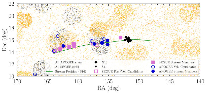
Figure 1: Spatial distribution of previously known 300S members, as well as the 300S candidates identified in this study. We also include all of the stars from the APOGEE (black) and SEGUE (orange) surveys in this patch of sky for reference. B16 reported that the stream spatial extent is slightly larger than the plotted stream track. However, we only include this section of the track because that is where the presence of the stream is most apparent.

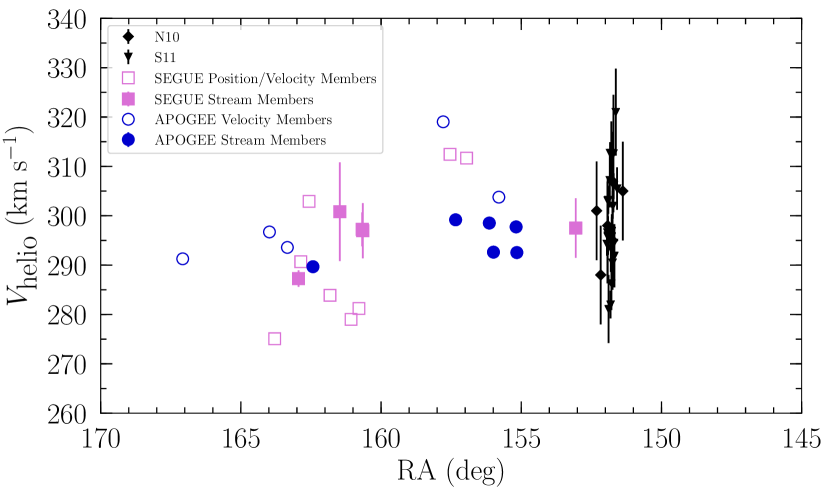
Figure 2: Velocity distribution of stream members and candidates as a function of RA. Since the stream runs approximately east-west, RA serves as a proxy for position along the stream. There may be a slight velocity gradient, with velocity decreasing as RA increases, but it is subtle.

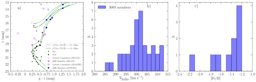
Figure 3: (a) CMD of the 300S members and APOGEE-2 and SEGUE candidates. Most of the new stars lie on the red giant branch, with one horizontal branch member from SEGUE. The symbols are the same as in Figure 1; the hollow symbols are stars that passed the velocity criterion, but failed the CMD selection. (b) Velocity distribution of the stream members selected from the two surveys, as well as from S11 and N10. Bins are 2 km s^-1 wide. (c) Metallicity distribution of stream members selected from the two surveys. Bins are 0.1 dex wide. There is a peak in metallicity at around $\mbox{[Fe/H]}=-1.4$, which is consistent with the metallicity measurement of one stream star by F13 and the photometric estimate from S11.

In order to obtain a reference isochrone against which to compare potential 300S members, we fit the known stream population from S11 and N10. For these stars, as for the rest of the stars in this study, we obtain their Pan-STARRS DR1 (PS1; Chambers et al., 2016) photometry, using the mean PS1 magnitudes, and apply extinction corrections using the Bayestar17 3D dust map and extinction laws of Green et al. (2018). A PARSEC isochrone (Marigo et al., 2017) with $\mbox{[Fe/H]}=-1.5$ and an age of 12 Gyr at a distance of 18 kpc is a good match to the known stream population, in agreement with the results from S11 and F13.

For the APOGEE-2 stars, we do an initial selection by examining their position on the color-magnitude diagram (CMD) shown in Figure 3a. B16 reported that the stream distance ranges from $14-19$ kpc. Because the stream distance near Segue 1 is 18 kpc, we posit that the stream distance increases toward smaller right ascension, and make a qualitative color selection based on identifying stars whose position on the CMD is close to, or in between, the best-fit isochrone shifted to distances of 14 kpc and 18 kpc.

The star 2M10231170+1608483 lacks PS1 and SDSS photometry, so we could not confirm its membership using its position on the CMD. The stars 2M10310815+1550149, 2M10555533+1409147, and 2M10532191+1638441 lie well away from the stream isochrone; 2M10532191+1638441 also lies too far north of the stream trace to be considered a member. After this photometric and kinematic selection, the majority of the stars lie along the trace of the stream from B16 (Figure 1), confirming for the first time that 300S is the kinematic counterpart of the photometric feature seen in B16. This association gives us an additional criterion for membership selection. In particular, the star 2M11081786+1018043 has colors consistent with it being a member of 300S, but falls several degrees beyond the trace of the stream from B16. It also falls outside of the track of the modeled orbit (see Section 4). For that reason, we also exclude it from 300S membership.

In summary, out of the 11 APOGEE stars that remain after the velocity selection, we reject 5 of them as 300S members for the following reasons: 1 lacks photometry, 3 lie far from the isochrone shifted to the appropriate distance, and 1 falls beyond the trace of the stream as shown in B16. All of these stars are represented in Fig 1 and on the CMD in Fig 3a as blue circles.

We then proceed to a more quantitative selection for photometric stream members. We approximate the distance gradient along the stream as varying linearly with right ascension ($\alpha$), where $(d/1~{}\mbox{kpc})=48.9952-0.2083\alpha$ and $\alpha$ is in degrees. The $y$-intercept and slope were determined by using the RA and distance measurements from B16, where we assume $d_{\rm 300S}=14$ kpc at $\alpha=168\arcdeg$, and $d_{\rm 300S}=19$ kpc at $\alpha=144\arcdeg$. Within the APOGEE-2 stars, we select photometric members of the stream by requiring that members be within 0.12 mag of the theoretical isochrone at its corresponding distance along the stream. Although the photometric uncertainties for these bright stars are quite small, we allow for a relatively wide selection window around the isochrone in order to account for uncertainties in our distance model and the stellar populations of the stream.

Table 1 provides the list of stars in APOGEE-2 that passed the spatial and velocity selection criteria. The stars that we consider members of 300S are marked with a “1” under the “MEM” field. Out of the 27 stars from APOGEE-2 in this patch of sky with $V_{\rm helio}>250$ km s^-1, 6 are ultimately members of 300S.

2.2 Stream Members in SEGUE-1, SEGUE-2

The SEGUE (Sloan Extension for Galactic Understanding and Exploration) 1 & 2 surveys collected $R\sim 1800$ spectra in the $3900-9000$ Å wavelength range for $\sim 240,000$ stars with $14<g<20.3$ across a wide range of spectral types (Yanny et al., 2009). The SEGUE data releases provide the radial velocity for every star, and, if the spectrum is of sufficient S/N, stellar atmospheric parameters such as metallicity, surface gravity, and effective temperature from the SEGUE Stellar Parameter Pipeline (SSPP) (Lee et al. 2008, Lee et al. 2008, Allende Prieto et al. 2008, Smolinski et al. 2011, Lee et al. 2011).

To search for 300S members from the SEGUE surveys, we begin by selecting stars in the region displayed in Figure 3 from B16 with velocities between 275 km s^-1 and 325 km s^-1, and with uncertainties of less than 10 km s^-1. To ensure that we do not have duplicate entries, we select stars that have the ‘scienceprimary’ flag set to 1. The spatial distribution of SEGUE stars with velocities near 300 km s^-1 does not obviously reveal the presence of the stream, so we make another spatial cut by selecting stars that are less than 0.75° away from the center of the stream trace shown in Figure 1. A total of 13 stars pass the velocity and position cuts, shown in Figures 1, 2 and 3 as pink squares.

In selecting for photometric members, we apply the same criterion described in Section 2.1, leaving 6 candidates. One of the stars, PSO J104717.120+145503.948, should lie on the RGB of the stream at an extinction-corrected $r$-band magnitude of 16.65. However, its atmospheric parameters determined from SEGUE spectroscopy, $T_{\rm eff}=5353$ K and $\log{g}=4.4$, suggest that it is a main sequence star. Thus, we exclude this star from the member sample.

The results of 300S member selection are shown in Figures 1, 2, and 3. Table 2 provides the list of stars in the SEGUE survey data that passed the spatial and velocity selection criteria. Table 3 provides the atmospheric parameters of the same stars, obtained from the publicly available SEGUE data. It also contains [Fe/H], [$\alpha$/Fe], and [C/Fe] abundance ratios derived from the updated SSPP described in Lee et al. (2011, $\alpha$-elements) and Lee et al. (2013, carbon). For these stars, the [Fe/H] measurements from the publicly available SEGUE data and from the updated SSPP pipeline are consistent with each other. In the rest of our analysis, we use the [Fe/H] measurements presented in Table 3. In both tables, the 5 stars that we consider members of 300S are marked with a “1” under the “MEM” field.

Table 1: 300S Candidate Members from APOGEE Data

APOGEE ID	RA	Dec	$V_{\rm helio}$	$\sigma_{V_{\rm helio}}$	[Fe/H]	$\sigma_{[Fe/H]}$	[C/Fe]	[C/Fe] (c.)	$g$	$r$	$i$	MEM
	($\degree$)	($\degree$)	(km s-1)	(km s-1)		(dex)			(mag)	(mag)	(mag)
2M10203784+1514471	155.15769	15.24642	292.54	0.01	$-$1.38	0.10	$-$0.57	$-$0.02	14.99	14.02	13.61	1
2M10204415+1555327	155.18399	15.92577	297.74	0.06	$-$1.24	0.10	$-$0.69	$-$0.45	16.02	15.36	15.03	1
2M10235791+1530589	155.99132	15.51638	292.62	0.13	…	…	…	…	17.40	16.83	16.57	1
2M10243358+1531009	156.13992	15.51694	298.52	0.04	$-$1.28	0.10	$-$0.50	$-$0.33	16.25	15.60	15.31	1
2M10292189+1520453	157.34122	15.34594	299.18	0.07	$-$1.32	0.10	$-$0.21	$-$0.18	16.22	15.67	15.41	1
2M10494291+1500530	162.42883	15.01473	289.68	0.01	$-$1.28	0.10	$-$0.65	$-$0.10	14.21	13.39	12.89	1
2M10231170+1608483	155.79876	16.14675	303.77	0.02	$-$1.20	0.10	$-$0.38	…	…	14.34	13.77	0
2M10310815+1550149	157.78400	15.83748	319.03	0.05	$-$1.00	0.10	$-$0.08	…	14.71	14.11	13.87	0
2M10532191+1638441	163.34129	16.64560	293.58	0.06	$-$1.14	0.10	$-$0.23	…	13.64	13.33	13.06	0
2M10555533+1409147	163.98056	14.15408	296.72	0.09	$-$1.39	0.10	$-$0.72	…	14.43	13.97	13.77	0
2M11081786+1018043	167.07442	10.30121	291.28	0.07	$-$1.07	0.10	$-$0.25	…	15.67	15.06	14.77	0

Note. — The 11 APOGEE-2 stars that meet the velocity criteria in the region of the stream trace found by B16. For easier direct comparison to the PS1 catalog, the PS1 magnitudes presented in this table have not been corrected for extinction.

Table 2: 300S Candidate Members from SEGUE Data

PS1 ID	RA	Dec	$V_{\rm helio}$	$\sigma_{V_{\rm helio}}$	[Fe/H]	$\sigma_{[Fe/H]}$	$g$	$r$	$i$	MEM
	($\degree$)	($\degree$)	(km s-1)	(km s-1)		(dex)	(mag)	(mag)	(mag)
PSO J101213.614+162336.187	153.05674	16.39340	297.5	6.0	$-$2.07	0.08	18.25	17.76	17.51	1
PSO J104236.584+150006.746	160.65240	15.00186	297.0	5.6	$-$1.45	0.08	19.24	18.82	18.64	1
PSO J104241.253+151913.286	160.67186	15.32034	297.2	3.4	$-$1.76	0.08	18.42	17.95	17.73	1
PSO J104552.952+144850.129	161.47066	14.81393	300.8	10.0	$-$1.43	0.04	19.45	19.23	19.17	1
PSO J105146.576+142850.068	162.94404	14.48055	287.3	1.7	$-$1.41	0.05	16.79	16.52	16.42	1
PSO J102747.821+151112.482	156.94925	15.18678	311.7	5.5	$-$1.44	0.24	17.48	17.55	17.64	0
PSO J103009.937+152241.212	157.54140	15.37809	312.4	5.3	$-$1.57	0.14	17.64	17.69	17.78	0
PSO J104309.200+152210.855	160.78830	15.36964	281.2	4.7	$-$1.33	0.04	18.83	18.52	18.40	0
PSO J104416.759+145459.165	161.06981	14.91639	279.0	6.1	$-$1.23	0.02	18.60	18.34	18.24	0
PSO J104717.120+145503.948	161.82127	14.91769	283.9	1.5	$-$1.43	0.06	17.21	16.73	16.52	0
PSO J105016.344+144644.466	162.56806	14.77903	302.9	2.8	$-$1.26	0.01	16.96	16.30	16.34	0
PSO J105127.367+144705.996	162.86398	14.78494	290.7	2.1	$-$1.83	0.02	16.23	16.01	15.95	0
PSO J105510.494+141100.053	163.79369	14.18334	275.1	6.4	$-$2.48	0.01	18.54	18.27	18.17	0

Note. — The stars from the SEGUE surveys that pass the spatial and velocity cut. For easier direct comparison to the PS1 catalog, the PS1 magnitudes presented in this table have not been corrected for extinction. The quoted metallicity uncertainties are SSPP internal errors; external uncertainties are 0.2 dex. PSO J101213.614+162336.187 is rather metal-poor compared to the other members. However, its velocity is consistent with membership in 300S.

2.3 Properties of Newly Identified Stream Members

As illustrated in Figure 3a, most of the 300S members appear to lie on the red giant branch. However, there is one star from the SEGUE survey that lies on the horizontal branch, which may be advantageous for determining a more robust distance measurement of the stream at a position away from Segue 1. The mean metallicity of the stream from these measurements is $\mbox{[Fe/H]}=-1.48$. For the SEGUE stars, we adopt an external metallicity uncertainty of 0.2 dex. For the APOGEE-2 stars, we adopt an external metallicity uncertainty of 0.1 dex. Using those values, we calculate an intrinsic metallicity dispersion of 0.21${}^{+0.12}_{-0.09}$ dex. Holtzman et al. (2015) note that the external uncertainty on ASPCAP [Fe/H] measurements ranges from 0.1 dex to 0.2 dex. The exact value that we adopt for the APOGEE-2 stars does not significantly affect our results because the metallicity dispersion is driven largely by the more metal-poor SEGUE stars. However, the choice of metallicity uncertainty for the SEGUE members does matter; a larger value can substantially reduce the derived intrinsic metallicity dispersion for 300S.

Figure 2 shows the heliocentric velocity of the stream members as a function of RA. There may be a slight velocity gradient along the stream, with velocity increasing with negative RA, but it is subtle. A larger sample size would be needed to verify the existence of the gradient.

For the 300S members in both the APOGEE-2 and SEGUE samples, we correct for the depletion of [C/Fe] along the red giant branch by applying the methods used in Placco et al. (2014). For the APOGEE-2 members, the respective carbon corrections for stars with available abundances (shown in the order in Table 1) are 0.55, 0.24, 0.17, 0.03, and 0.55 dex. We present the corrected values in Table 1. For the SEGUE stars, the corrected carbon abundances are included in Table 3. For these stars, the corrections are less than 0.1 dex. One 300S star, PSO J104236.584+150006.746, can be classified as carbon-enhanced ($\mbox{[C/Fe]}=+0.90$). Given its metallicity, PSO J104236.584+150006.746 is likely a CEMP-$s$ star enriched by a binary companion. Follow-up spectroscopy to measure its neutron-capture element abundances and velocity variability may be interesting to confirm this possibility.

Table 3: Atmospheric Parameters and Abundances for 300S Candidates Members from SEGUE

PS1ID	$T_{\mbox{eff}}$	$\sigma_{T_{\mbox{eff}}}$	$\log{g}$	$\sigma_{\log{g}}$	[Fe/H]	$\sigma_{\mbox{[Fe/H]}}$	[$\alpha$/Fe]	$\sigma_{\mbox{[$\alpha$/Fe]}}$	[C/Fe]	$\sigma_{\mbox{[C/Fe]}}$	[C/Fe] (c.)	MEM
	(K)	(K)		(dex)		(dex)		(dex)		(dex)
PSO J101213.614+162336.187	5057	83	2.3	0.1	$-$2.17	0.13	$+$0.85	0.17	$-$0.26	0.12	$-$0.26	1
PSO J104236.584+150006.746	5367	47	2.6	0.1	$-$1.65	0.11	$+$0.28	0.22	$+$0.88	0.11	$+$0.90	1
PSO J104241.253+151913.286	5216	63	2.5	0.1	$-$1.75	0.13	$+$0.39	0.15	$+$0.04	0.10	$+$0.06	1
PSO J104552.952+144850.129	6557	53	4.0	0.6	$-$1.26	0.20	$+$0.21	0.20	$+$0.57	0.42	$+$0.57	1
PSO J105146.576+142850.068	6131	62	2.3	0.3	$-$1.45	0.07	$+$0.43	0.08	$-$0.12	0.22	$-$0.10	1
PSO J102747.821+151112.482	8275	22	4.1	0.2	$-$1.56	0.11	…	…	…	…	…	0
PSO J103009.937+152241.212	7970	76	4.0	0.1	$-$1.49	0.08	…	…	$+$2.19	0.5	$+$2.20	0
PSO J104309.200+152210.855	6047	55	4.2	0.1	$-$1.30	0.02	$+$0.31	0.16	$+$0.21	0.14	$+$0.21	0
PSO J104416.759+145459.165	6313	53	3.3	0.2	$-$1.27	0.11	$+$0.26	0.20	$+$0.58	0.28	$+$0.59	0
PSO J104717.120+145503.948	5353	17	4.4	0.0	$-$1.44	0.04	$+$0.46	0.04	$+$0.04	0.02	$+$0.04	0
PSO J105016.344+144644.466	6590	105	3.2	0.2	$-$1.46	0.07	$+$0.67	0.10	$+$0.46	0.16	$+$0.48	0
PSO J105127.367+144705.996	6453	32	3.7	0.1	$-$1.87	0.06	$+$0.54	0.14	$<$0.01	…	…	0
PSO J105510.494+141100.053	6329	56	3.8	0.2	$-$2.75	0.12	$+$0.64	0.15	$+$1.66	0.42	$+$1.66	0

Note. — Atmospheric parameters and [Fe/H], [$\alpha$/Fe], and [C/Fe] abundances for the 11 SEGUE stars that pass the spatial and velocity cuts. $T_{\mbox{eff}}$ and $\log{g}$ were obtained from the publicly available SEGUE data, while the abundance measurements were obtained using the updated SSPP, described in Lee et al. (2011, $\alpha$-elements) and Lee et al. (2013, carbon). The column “[C/Fe] (c.)” provides the carbon abundances of these stars, corrected for evolutionary stage using the methods described in Placco et al. (2014). The uncertainties quoted are SSPP internal errors. External uncertainties in $T_{\rm eff}$, $\log{g}$, [Fe/H], [$\alpha$/Fe] and [C/Fe] are 125 K, 0.35 dex, 0.2 dex, 0.2 dex and 0.25 dex respectively. The star PSO J104236.584+150006.746 can be classified as carbon-enhanced ($\mbox{[C/Fe]}=+0.90$); given its metallicity, it is likely a CEMP-$s$ star.

3 Chemical Abundance Analysis

In this section we examine the chemical abundances of the stream members identified in Section 2. We analyze detailed abundances for the six APOGEE-2 stream members identified in Section 2.1. For one of these stars, 2M10235791+1530589, the ASPCAP pipeline was unable to determine any abundances. However, a line-by-line analysis of its spectrum suggests similar abundances to the other five stars. We also examine the [$\alpha$/Fe] abundance ratios for the SEGUE stream members.

3.1 Comparison Sample Selection

From the APOGEE-2 dataset, we select various other sets of stars with which to compare chemical abundances. For all stars, we verify that none have the ‘STAR_BAD’ ASPCAP flag, which encodes any unreliable ASPCAP measurements, set (Holtzman et al., 2015). We also ensure that these stars have internal uncertainties less of than 0.2 dex for each element considered.

For a dwarf galaxy comparison sample, we select members of the Sagittarius (Sgr) dwarf galaxy from APOGEE (see Hasselquist et al. 2017 for a detailed study of the chemical abundances of Sagittarius). We begin by selecting stars with the ‘APOGEE_SGR_DSPH’ flag set in the APOGEE_TARGET1 column. From that sample, we apply a velocity cut, selecting stars with $120~{}\mbox{km\,s${}^{-1}$}<V_{\rm helio}<160$ km s^-1, which isolates most stars in the core and removes some potential contaminants. For data on other dwarf galaxies, we use the measurements of Shetrone et al. (2003) for Sculptor, Leo I, Carina and Fornax, Cohen & Huang (2009) for Draco, and Cohen & Huang (2010) for Ursa Minor.

We also select APOGEE stars in the globular clusters M13 and M92 for comparison. We chose M13 because its metallicity is similar to that of the stream, and M92 as a metal-poor reference. We take cluster membership information from Mészáros et al. (2015). However, we use chemical abundances from ASPCAP to control for potential systematics due to different analysis methods.

We construct our halo sample by obtaining distances from the APOGEE DR14-Based Distance Estimations value added catalog, which was constructed using the isochrone matching technique (NICE; Schultheis et al., 2014). To determine the height above the Galactic plane where 90% of the stars are from the halo as a function of Galactocentric radius, we use the Trilegal model (Vanhollebeke, Groenewegen, & Girardi, 2009). This height varies from  3 to 10 kpc as a function of radius.

We also supplement our position-selected halo sample with stars that have 3D space motions consistent with halo membership, which we base on Gaia DR1 proper motions (see Gaia Collaboration et al. 2016, Brown et al. 2016, Lindegren et al. 2016, and Arenou et al. 2017, among others) and APOGEE DR14 radial velocities. We select our stars as those that have rotational and $UW$ velocities that differ from those of thick- and thin-disk stars by more than 2$\sigma$. Due to the magnitude limits in Gaia DR1, there was very little overlap between these two differently selected samples.

3.2 Light-Element Abundance Correlations

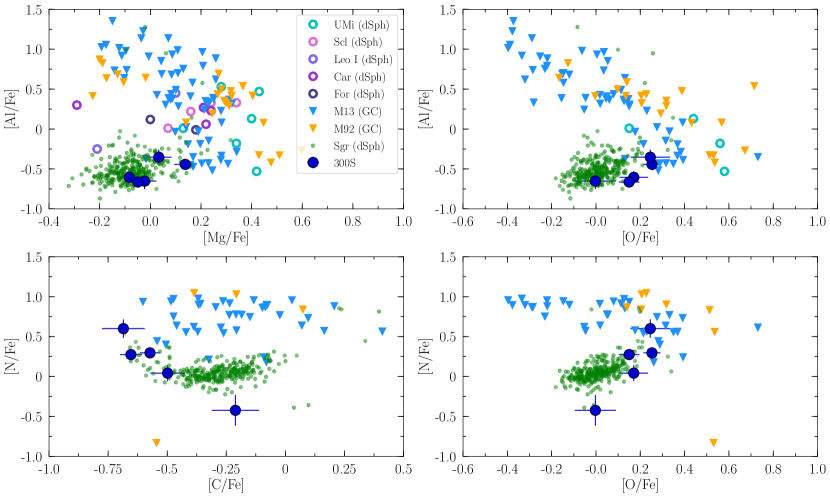
Figure 4: Light-element abundance ratios of 300S stars (filled blue circles) in comparison to globular clusters and dwarf galaxies. Data for UMi are from Cohen & Huang (2010). Data for the other dwarf spheroidals (dSphs), not including Sgr, are from Shetrone et al. (2003). 300S does not follow the light-element correlations seen in globular clusters. Instead, its abundance pattern resembles Sgr.

We begin our investigation into the nature of the stream progenitor by comparing its chemical abundance pattern to those of globular clusters. Globular cluster stars obey well-known correlations between abundances of light elements including carbon, nitrogen, oxygen, sodium, aluminum, and magnesium (see, e.g., Gratton et al., 2004, and references therein). In Figure 4 we examine the light-element abundances of 300S in comparison to M92 and M13, as well as to Local Group dwarf galaxies. Because Na is too weak to be measured in the $H$-band at low metallicity ($[\mathrm{Na/H}]\lesssim-1$), we could not test for a Na-O anti-correlation among the 300S stars.

It is apparent that members of 300S do not display the chemical abundance correlations of globular clusters, either in the direction of the correlation or the shape of the distribution. From comparison with Figure 9 of Mészáros et al. (2015), which shows the Mg-Al correlations of the globular clusters from that study, we note in particular that 300S does not resemble either the first-generation or second-generation stars in M13. The chemical abundances of 300S are also much more similar to those of the Sagittarius dwarf galaxy than either of the globular clusters. This comparison strongly suggests that the progenitor of 300S is more likely to be a dwarf galaxy than a globular cluster.

3.3 [C/N] Ratio

To first order, the [C/N] ratio serves as an indicator of age. In Figure 5 we compare the [C/N] ratios of 300S to those of Sagittarius and the Milky Way halo. To control for evolutionary stage and possible deviations from local thermodynamic equilibrium (LTE), we select stars from our comparison sample that have similar $\log{g}$ and [Fe/H] to 300S. In the regime of $-1.5<\mbox{[Fe/H]}<-1.0$, the 300S members appear to be approximately as old as Sgr and the halo.

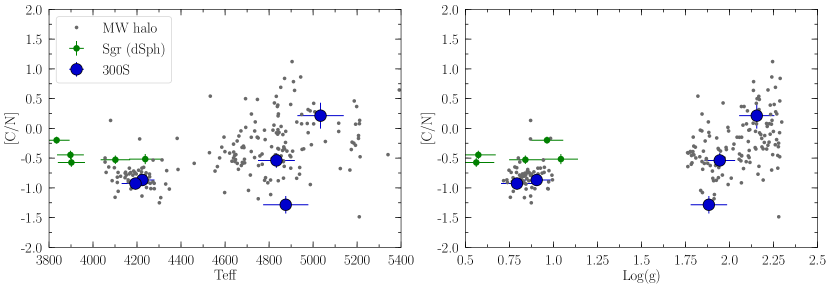
Figure 5: Comparison of the [C/N] ratio of 300S stars to that of Sgr and MW halo stars with similar metallicity and $\log{g}$. In the range of $-1.5<\mbox{[Fe/H]}<-1.0$, 300S looks similar to both Sgr and the MW halo, suggesting that they are approximately of the same age.

3.4 Chemical Abundance Patterns

To control for non-LTE effects, we originally only selected stars that are similar to the 300S sample in $T_{\rm eff}$ and $\log{g}$. However, the conclusions we drew from considering only such $T_{\rm eff}$ and $\log{g}$ “twins” were the same as those from considering the full halo sample. Therefore, we present our full sample of halo stars in the following figures in order to better illustrate the halo chemical abundance distribution, and highlight the stars that are $T_{\rm eff}$ and $\log{g}$ twins of 300S.

Figure 6 compares the [$\alpha$/Fe] abundance ratios of 300S to those of Sgr, the MW halo, and Ursa Minor. To ensure a consistent comparison to the [$\alpha$/Fe] ratios for the SEGUE stars, we calculate [$\alpha$/Fe] for the other populations by taking a weighted average abundance of Mg, Ca, Ti, and Si, where the weights for these four elements are given in Lee et al. (2011). For Ti, we give the same weight to the abundances of its different ionization states. Ursa Minor was the only dSph from the literature included in this sample, because it alone has published abundances for all four of the above-mentioned elements. The “knee” of the [$\alpha$/Fe] ratio as a function of metallicity (Tinsley, 1979) for 300S appears to occur at around [Fe/H] = $-1.3$. 300S reaches solar [$\alpha$/Fe] at a similar metallicity to the classical dSphs.

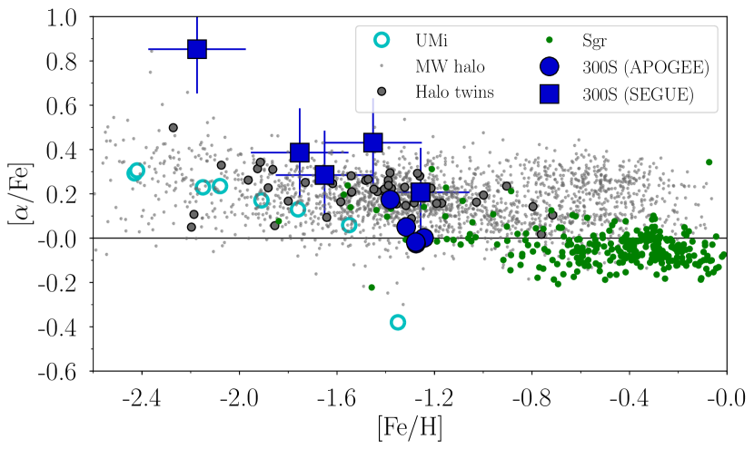
Figure 6: Comparison of [$\alpha$/Fe] ratio of 300S stars to that of Sgr and MW halo stars, as well as to Ursa Minor. MW halo stars that are $T_{\rm eff}$ and $\log{g}$ twins of 300S are shown as solid gray circles with black outlines. The error bars on the SEGUE data points are based on their external uncertainties. The stars in 300S appear to reach solar levels of [$\alpha$/Fe] at around [Fe/H] = $-1.3$, which is between the respective metallicities where Ursa Minor and Sagittarius reach solar [$\alpha$/Fe] levels.

Figure 7 compares individual $\alpha$-elements as a function of metallicity in 300S and Sgr. The $\alpha$-element abundances of 300S generally match those of the classical dSphs. 300S may be slightly enriched in calcium compared to Sgr and the other dwarf spheroidals. Compared to the MW halo, 300S also seems to have similar $\alpha$-element abundances.

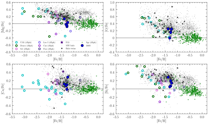
Figure 7: The $\alpha$-element abundance ratios as a function of metallicity for 300S stars compared to those of the halo and other Milky Way satellites. Data for UMi and Draco are from Cohen & Huang (2010) and Cohen & Huang (2009), respectively. Data for the other dSphs, not including Sgr, are from Shetrone et al. (2003). MW halo stars that are $T_{\rm eff}$ and $\log{g}$ twins of 300S are shown as solid gray circles with black outlines. We also include the 300S member analyzed in F13, shown as the purple star when relevant. Overall, 300S displays similar $\alpha$-element abundances to those of the Local Group dwarf galaxies and the MW halo.

Figure 8 compares the abundances of Fe-peak elements in 300S to those of the other Milky Way systems. 300S appears to be deficient in Cr relative to the other dwarf spheroidals. Within the uncertainties, 300S has similar Mn and Ni abundances to the dwarf galaxies. Overall, 300S has similar Fe-peak abundance patterns relative to the MW halo. Compared to the reference globular clusters, 300S is deficient in Fe-peak elements.

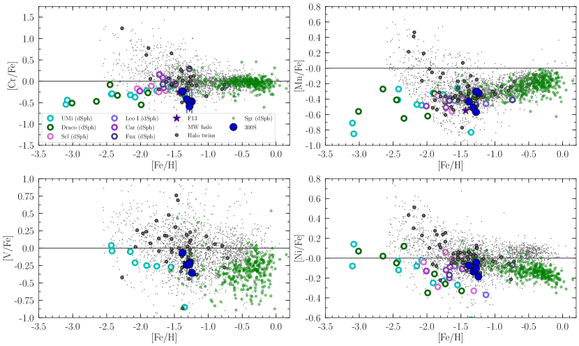
Figure 8: The Fe-peak element abundance ratios for 300S stars relative to those of Milky Way systems. Data for other dwarf galaxies in these plots are from the same studies cited previously. MW halo stars that are $T_{\rm eff}$ and $\log{g}$ twins of 300S are shown as solid gray circles with black outlines.

That 300S has similar chemical abundance patterns to the Milky Way halo, as well as dSphs, and different ones from those of globular clusters, further suggests that the 300S progenitor is a dwarf galaxy.

4 Tidal Disruption History

4.1 Proper Motion Modeling

In Section 2, we determined the path of 300S along the sky and its distance and velocity as a function of position. In order to calculate the orbit of the stream around the Milky Way, we also require proper motions.

We initially attempted to employ proper motion catalogs such as UCAC5 (Zacharias et al., 2017), and the recently released GPS-1 (Tian et al., 2017), to constrain the proper motions of the stream members. However, we found that the published proper motions of the APOGEE-2 and SEGUE stars in the stream exhibit a large scatter, and the UCAC5 and GPS-1 proper motions are not in very good agreement for the stars with measurements in both catalogs. Table 4 presents the catalog proper motion values for the members of 300S identified in Section 2.

Table 4: Proper motions for 300S Members from UCAC5, GPS-1

StarID	$\mu_{\alpha,GPS1}\cos{\delta}$	$\sigma$	$\mu_{\delta,GPS1}$	$\sigma$	$\mu_{\alpha,UCAC5}\cos{\delta}$	$\sigma$	$\mu_{\delta,UCAC5}$	$\sigma$
	(mas yr-1)	(mas yr-1)	(mas yr-1)	(mas yr-1)	(mas yr-1)	(mas yr-1)	(mas yr-1)	(mas yr-1)
2M10203784+1514471	-5.7	3.0	-2.7	2.5	…	…	…	…
2M10204415+1555327	-5.7	1.7	-1.4	1.3	…	…	…	…
2M10235791+1530589	-0.4	1.4	0.0	1.2	…	…	…	…
2M10243358+1531009	-2.4	1.3	-7.7	1.2	-6.5	3.8	-3.4	2.7
2M10292189+1520453	0.0	1.5	0.2	1.2	…	…	…	…
2M10494291+1500530	0.0	3.0	-8.3	2.6	-4.8	1.1	-4.5	1.1
PSO J101213.614+162336.187	-1.9	1.7	-1.8	1.2	…	…	…	…
PSO J104236.584+150006.746	-3.5	1.9	-2.7	1.5	…	…	…	…
PSO J104241.253+151913.286	-6.4	1.8	-6.1	1.8	…	…	…	…
PSO J104552.952+144850.129	-3.4	2.1	-1.6	1.7	…	…	…	…
PSO J105146.576+142850.068	-1.5	1.4	-4.4	1.4	-8.9	14.9	1.0	9.7

Note. — Proper motions for the new 300S stars, obtained from the GPS-1 and UCAC5 catalogs. Directly to the right of every proper motion measurement is its corresponding measurement uncertainty.

Thus, we instead infer the proper motion of the stream by considering many possible orbits subject to the constraints of its known properties. We test a grid covering the full range of plausible proper motions to see which of them produce a stream with (1) the observed path, constrained by B16, (2) the distance along the stream, which we were able to obtain for APOGEE-2 stars from Queiroz et al. (2018), and (3) the velocity along the stream, constrained by the APOGEE-2 and SEGUE 300S members.

We model 300S using the open-source code galpy (Bovy, 2015), and approximate the orbit of the stream using point-particle integration. We integrate the orbits in the MWPotential2014 potential, which is the standard Milky Way model in galpy, and adopt the solar motion from Schönrich et al. (2010). In order to initialize an orbit, galpy requires 6D phase space information about the point where the orbit is initialized. We initialize the orbit of 300S at the location of the S11 stars (i.e., Segue 1) because that region has the best-constrained values as a result of the large sample of confirmed main sequence member stars. At that location, $\alpha=151.8\arcdeg$, $\delta=16.1\arcdeg$, $V_{\rm helio}=298.8$ km s^-1, and $D_{\odot}=18$ kpc (S11).

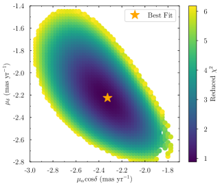
Figure 9: Reduced $\chi^{2}$ value of the best-fitting orbit (DOF=72). The best-fit $\mu_{\alpha}\cos{\delta}$, $\mu_{\delta}$ values are $-$2.33 mas yr^-1and $-$2.22 mas yr^-1, respectively. The orbit from those proper motions has a reduced $\chi^{2}$ value close to 1, suggesting that the orbit model is a good fit to the data.

For every orbit corresponding to a proper motion, we compute its $\chi^{2}$ value based on its fit to the stream observables. Since the velocity errors for APOGEE are very small (Nidever et al., 2015), we calculate $\chi^{2}$ for the APOGEE velocities assuming a Gaussian dispersion of 3 km s^-11 as a reasonable velocity dispersion for a stellar stream (Newberg et al. 2010, Casey et al. 2013). The velocity dispersion of the stream further away from Segue 1 is not well-constrained (see Section 5), so we allow for the possibility of a velocity dispersion without deviating too far from the measured values. We estimate the width of the stream to be 0.94 degree, and, assuming that our points are roughly centered on the stream, adopt a Gaussian dispersion of 0.47 degree for our on-sky spatial uncertainty.

Figure 9 shows the results of the $\chi^{2}$ fits for a region around the best fit proper motion. The proper motion of the orbit corresponding to the lowest $\chi^{2}$ fit is $\mu_{\alpha}\cos{\delta}=-$2.33 mas yr^-1, and $\mu_{\delta}=-$2.22 mas yr^-1. The reduced $\chi^{2}$ value of the orbit fit at those proper motions, with a DOF of 72, is close to 1, suggesting that the model is a good fit. This proper motion is also close to the weighted mean of the GPS-1 proper motions of the member stars ($\mu_{\alpha}\cos{\delta}=-2.5\pm 0.5$ mas yr^-1, $\mu_{\delta}=-2.8\pm 0.4$ mas yr^-1), despite the large uncertainties of many of the individual measurements.

For completeness, we fit an orbit with a positive $\mu_{\alpha}$, where the stream would travel in the opposite direction, and obtain proper motions of $\mu_{\alpha}\cos{\delta}=1.48$ mas yr^-1, and $\mu_{\delta}=-2.63$ mas yr^-1. This orbit has a distance vs. $RA$ gradient that points in the opposite direction of the negative $\mu_{\alpha}$ solution. This orbit also has a corresponding reduced $\chi^{2}$ value of 2.15, suggesting that the positive $\mu_{\alpha}$ orbit is a poorer fit to the data, and is on a lower eccentricity orbit with a larger perigalactic distance of 17 kpc.

Thus, we prefer the negative $\mu_{\alpha}$ solution due to its better agreement with the GPS-1 proper motions, and because its much smaller perigalactic distance is more consistent with the observed disruption of the stream progenitor. The forthcoming Gaia DR2 measurements will eliminate this degeneracy.

4.2 Properties of the Modeled Orbit

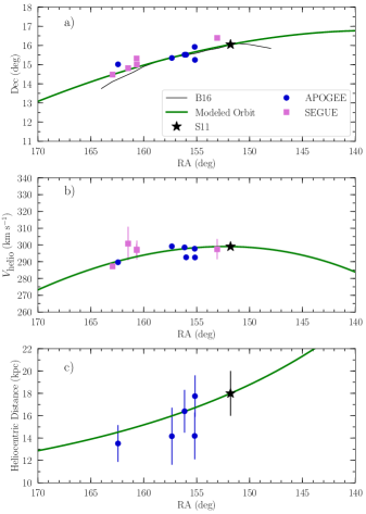
Figure 10: (a) Modeled orbit of the stream compared to its observed position on the sky. The orbit passes through the position of the known members, but deviates slightly from the trace of the stream as seen in B16. (b) Modeled heliocentric velocity along the stream track. The modeled orbit is in good agreement with the data. (c) Modeled distance along the stream. Distances plotted are to the APOGEE-2 stream members according to Queiroz et al. (2018). The modeled orbit is consistent with all of the distance measurements to within $2\sigma$.

The panels in Figure 10 compare the modeled orbit with the observed properties of the stream. In Figure 10a, the position of the modeled orbit is consistent with the location of the 300S members. The orbit also does not pass close to the position of 2M11081786+1018043, corroborating our decision in Section 2.1 that the star is not a likely 300S member. In Figure 10b and 10c, the modeled orbit is consistent with the heliocentric velocity and distance along the stream track. Although the orbit deviates slightly from the trace of the stream as seen in B16, it is still reasonable to use it to infer general features of the stream’s kinematic history.

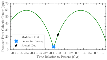
Figure 11: Galactocentric distance of the stream orbit as a function of time. The stream passed perigalacticon about 70 Myr ago, approaching within $\sim$4.1 kpc of the Galactic Center.

Figure 11 shows the distance of the stream away from the Galactic Center as a function of time, suggesting that the progenitor of 300S passed perigalacticon only $\sim$ 70 Myr ago. At its closest approach, the progenitor was $\sim$4.1 kpc from the Galactic Center, and thus must have experienced powerful tidal forces.

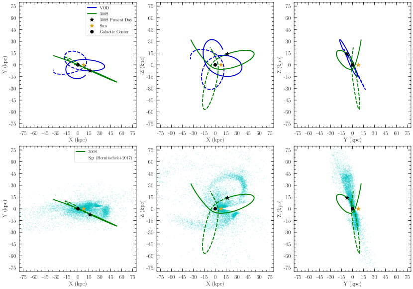
Figure 12: Modeled orbit of 300S (green curve) projected onto various Cartesian frames centered at the Galactic Center, illustrating the high eccentricity of the stream’s orbit. The top row compares the orbit of 300S with the Virgo Overdensity (VOD), using the data from Carlin et al. (2012). The results of this orbit suggest a possible association between 300S and VOD. The second row compares the orbit of 300S with the observed portions of Sagittarius as seen in Hernitschek et al. (2017). These results affirm the conclusion of previous studies that Sgr and 300S are unlikely to be kinematically related. More detailed data and modeling would be needed to further ascertain the relationship of 300S to these two substructures.

Figure 12 shows the modeled orbit projected onto various Cartesian planes centered on the Galactic Center, compared to the orbit of the Sagittarius dwarf spheroidal galaxy (bottom row, observed data from (Hernitschek et al., 2017)) and to that of the Virgo Overdensity (VOD; observed parameters from Carlin et al., 2012). The orbit of 300S does not resemble that of Sgr (also see Law & Majewski, 2010), supporting previous suggestions that 300S is unlikely to be kinematically associated with the Sagittarius stream (G09, S11, B16). If the two are related, the 300S progenitor must have been stripped from Sgr long ago. However, the orbit of VOD appears to pass close to 300S, supporting Carlin et al. (2012)’s suggestion that the two substructures could share a common origin. Finally, the orbit of the stream is perpendicular to the proper motion of Segue 1 (Fritz et al., 2017), ruling out any association with that galaxy.

4.3 Integrated Luminosity of the Stream

In order to place a lower limit on the original mass of the core of the progenitor, we calculate the integrated luminosity of the stream using PS1 photometry (Chambers et al., 2016). We follow the same procedures outlined in B16 to select stellar-like objects. In particular, we select sources with $|r_{\rm psf}-r_{\rm aperture}|\leq 0.2$ mag. To ensure the quality of our photometry, we also reject sources with uncertainties larger than 0.2 mag in $g$, $r$, and $i$ bands. We correct for reddening effects using the dust maps of Schlegel et al. (1998) and the extinction law of Schlafly & Finkbeiner (2011).

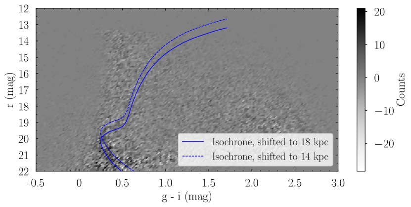
Figure 13: Background-subtracted Hess diagram of 300S, where the main sequence of the stream is apparent. The isochrone overplotted at different distance is the same as that in Figure 3a.

We create a Hess diagram of 300S by subtracting a matching Hess diagram of the Milky Way foreground population from the Hess diagram of the region within the stream. The width of the stream is $\sim 1\arcdeg$ (see Section 5). Thus, to construct our foreground distribution, we consider two regions. At a distance of 1° north of the center of the stream, we obtain the foreground distribution by using the stars within a region of sky that is 1° wide and runs parallel to the stream track. At a distance of 1° south of the stream center, we construct another foreground distribution in an analogous fashion. We average the distributions from the regions above and below the stream to produce the foreground Hess diagram, and subtract that from the Hess diagram of the region within the stream. We present the 300S Hess diagram in Figure 13, along with the isochrone of 300S overplotted at 14 and 18 kpc for comparison.

From the foreground-subtracted Hess diagram, we find a total of 637 stars within the stream down to a magnitude of $r=22$. For comparison, Martin et al. (2008) measured 65 stars in Segue 1 ($L=335$ L_⊙) down to the same magnitude limit in SDSS. In each Hess diagram bin along the stream CMD sequence we calculate a luminosity using the isochrone described in Section 2.1 and shown in Figure 3a. After correcting for the contribution of sources below the PS1 magnitude limit following Martin et al. (2008), we obtain an integrated luminosity for 300S of $4\times 10^{3}$ L_⊙.

Since the chemical abundances of the stream stars suggest that the progenitor of 300S is a dwarf galaxy, we can invoke the mass-metallicity relationship for dwarf galaxies (Kirby et al., 2013) to infer a progenitor stellar mass of $10^{6.9\pm 0.6}$ M_⊙, which is on the order of a classical dwarf galaxy (e.g., Leo I, Sculptor). The implied luminosity of this stellar mass is far greater than the observed luminosity of the stream. This suggests that the 300S progenitor was either abnormally metal-rich for its luminosity, or that most of its mass was stripped earlier and is not present in the currently-known part of the stream.

5 The Origin of 300S

Until the discovery of the ultra-faint dwarf galaxies in 2005 (Willman et al., 2005a, b), globular clusters and dwarf galaxies exhibited clearly distinct structural properties, with all dwarf galaxies having radii of more than 100 pc and all globular clusters having radii less than 30 pc (e.g., Belokurov et al., 2007). Over the last decade the size distributions of the two populations have begun to encroach upon one another at faint luminosities ($L\lesssim 10^{4}$ L_⊙), such that size alone is no longer sufficient to classify compact stellar systems. This convergence has led to the adoption of alternative classification criteria, namely dynamical mass-to-light ratio and metallicity dispersion (Willman & Strader, 2012). While the interpretation of the stellar kinematics is rendered more difficult in the case of a tidally disrupted object, the chemical properties of the stars are preserved during the disruption process.

To ascertain the nature of the 300S progenitor, we first consider the chemical abundance measurements presented in Sections 2 and 3. The metallicites of the APOGEE-2 member stars are all quite similar to each other (and to 300S-1 from F13). However, the SEGUE members span a range in metallicity from $\mbox{[Fe/H]}=-1.3$ to $-2.2$, such that the intrinsic dispersion of the metallicity distribution for our full sample of new members is 0.21${}_{-0.09}^{+0.12}$ dex. While we cannot distinguish this value from zero with high statistical significance, the data do suggest that 300S is not a mono-metallic system. Although the sample size is small, we also do not see any sign of the characteristic globular cluster light-element abundance correlations in 300S. With detailed abundance patterns for only five stars, we cannot exclude the possibility that all of the APOGEE-2 stars happen to belong to a single stellar generation and that high-resolution spectroscopy of additional stars would reveal multiple populations with correlated abundances. While each individual piece of evidence is not a strong indicator of the nature of the progenitor, taken together, the best explanation for the data is that the progenitor of 300S was a dwarf galaxy.

To constrain the size of the stream progenitor, we estimate the width of the stream. The profile of the stream perpendicular to its length has a full-width at half maximum of 0.94°, corresponding to a physical extent of $\sim 260$ pc at an average distance of 16 kpc. This size is consistent with the hypothesis that the progenitor was a relatively compact dwarf galaxy.

S11 measured a velocity dispersion for the stream at the position of Segue 1 of $7.0\pm 1.4$ km s^-1 with all candidate member stars included, and $5.6\pm 1.2$ km s^-1 if several possible foreground stars are excluded. Because the best-fit stream model we computed in Section 2 indicates that there may be a velocity gradient of $\sim 10$ km s^-1 across the full region spanned by the spectroscopic data, we cannot simply use the entire sample of member stars to calculate the velocity dispersion. Instead, we use the fact that the five of the six APOGEE-2 stars and four of the five SEGUE stars are clustered together (near $\alpha_{2000}=156\arcdeg$ and $\alpha_{2000}=161.5\arcdeg$, respectively) to determine local velocity dispersions at these two positions. The dispersion of the APOGEE-2 stars near $\alpha_{2000}=156\arcdeg$ is $\sigma=3.3^{+1.8}_{-1.1}$ km s^-1, while that of the SEGUE stars near $\alpha_{2000}=161.5\arcdeg$ is $\sigma=5.1^{+4.8}_{-2.8}$ km s^-1. Within the uncertainties, we therefore conclude that the data are consistent with the stream having a constant velocity dispersion of $\sim 4-5$ km s^-1 over the RA range $\alpha_{2000}=151.8\arcdeg-161.5\arcdeg$. Recognizing that the disruption of the progenitor may have resulted in a stream velocity dispersion that is higher than that of the progenitor system, we note that this dispersion is larger than that of the prototypical globular cluster stream Pal 5 (Odenkirchen et al., 2009; Kuzma et al., 2015).

Finally, we consider the stream orbit derived in Section 4. The path of the stream indicates that it is moving on a highly elliptical orbit. Such an orbit would be quite unusual for a globular cluster (e.g., Dinescu et al., 1999; Allen et al., 2006). More eccentric orbits are expected for dwarf galaxies, which may have fallen into the Milky Way from large distances, as opposed to forming in situ like many globular clusters. Orbits approaching within a few kpc of the Galactic Center are likely not common for dwarfs either, but very small perigalacticon distances are necessary in order to completely disrupt a dark matter-dominated system. As an example, S11 calculated that a galaxy with the mass and size of Segue 1 would need to pass within $\sim 4$ kpc of the Galactic Center to be disrupted.

We conclude that the observed properties of 300S favor a dwarf galaxy, rather than a globular cluster, progenitor. Next, we examine some of its characteristics in the context of other dwarf galaxies. If we invoke the mass-metallicity relation for dwarf galaxies (Kirby et al., 2013), the metallicity of the stream corresponds to a progenitor stellar mass of $10^{6.9\pm 0.6}$ M_⊙, which is comparable to a classical dwarf spheroidal galaxy such as Leo I (${\rm[Fe/H]}=-1.43$). That 300S reaches solar levels of [$\alpha$/Fe] at a metallicity between that of Ursa Minor and Sgr also suggests that the stellar mass of its progenitor is between $2\times 10^{5}$ M_⊙ (UMi) and at least $2\times 10^{7}$ M_⊙ (Sgr, core). Using Equation 28 from Erkal et al. (2016), which calculates the mass of the stream progenitor from the width of the stream on the sky and the enclosed mass at the stream distance, we obtain a progenitor mass of $10^{5.3}$ M_⊙. However, the integrated luminosity of the stream over its observed extent is only $4000$ L_⊙. Reconciling these numbers requires either that the progenitor dwarf was unusually metal-rich (and perhaps unusually extended) for its luminosity, that the progenitor was strongly dark-matter dominated, or that nearly all of the stars belonging to the progenitor lie outside the known stream. Since the stream’s orbit extends out to nearly 60 kpc, where most of its stars would be too faint to be detected by current surveys, the latter scenario may be plausible. In addition, it is possible that the progenitor made previous close passages to the Galactic Center during which most of its mass was lost. Given the derived orbital period of $\sim 1$ Gyr (see Fig. 11), such stars could now be located quite far away from 300S.

The origin of 300S could be connected with other known substructures. While the orbit of 300S is not perfectly coincident with that of VOD, their similarity suggests that that the two substructures could share a common origin. Carlin et al. (2012) estimated a progenitor mass of $10^{9}M_{\odot}$ for VOD, so 300S may have fallen into the Milky Way with a more massive companion. Cosmological simulations indicate that $\sim 30-60$% of dwarf satellites around MW-like halos were accreted as members of galaxy groups (Wetzel et al., 2015); thus, the phenomenon of group infall more generally is not unlikely. Although the radial velocity and orbit shape of 300S are not consistent with the known portions of the Sgr stream (G09), the spatial overlap between the two and their chemical similarity suggests the possibility that the stream progenitor might once have been a dwarf satellite of Sagittarius. Previous wraps of Sgr debris around the Galaxy are not well-constrained by existing data, so an association with Sgr cannot currently be ruled out observationally. For both VOD and Sgr, improved proper motion measurements and more detailed modeling of the early history of their interaction with the Milky Way would be needed to understand their relationship to 300S.

6 Conclusions

In this study, we present 11 new members of 300S identified in the APOGEE-2 and SEGUE spectroscopic surveys. From the position of these stars on the sky, we show that 300S is the kinematic counterpart of the elongated photometric substructure found in the same region.

We find that the 300S members from APOGEE-2 are chemically similar to Local Group dwarf galaxies and the Milky Way halo, and do not display the characteristic light-element abundance correlations of globular clusters. The new known members also display a metallicity dispersion of 0.21${}_{-0.09}^{+0.12}$ dex, exceeding an intrinsic dispersion of 0 by 2 $\sigma$. This suggests that the progenitor may have had an extended period of star formation and a potential well sufficiently deep to retain supernova ejecta. The relatively large width and velocity dispersion of the stream also point to a massive progenitor. Thus, we conclude that 300S is likely the remnant of a tidally disrupted dwarf galaxy.

We infer the proper motion of the stream by fitting the observed properties of the stream to orbits generated from a grid of possible proper motions. The best-fit orbit is highly eccentric, with an apogalacticon distance of 60 kpc and perigalacticon distance of 4.1 kpc away from the Galactic Center. The orbital period of 300S is $\sim 1$ Gyr, with its most recent perigalacticon passage 70 Myr ago.

Invoking the mass-metallicity relationship for dwarf galaxies, we find that the progenitor of 300S should have a stellar mass of $10^{6.9\pm 0.6}$ M_⊙, which is comparable to classical dwarf spheroidal galaxies such as Leo I, Sculptor, and Fornax. We also calculate the integrated luminosity of the stream to be $4\times 10^{3}$ L_⊙, which is much lower than the luminosity implied by the stellar mass from the previous relation. However, at a perigalacticon distance of 4.1 kpc, the tidal field of the Milky Way is sufficiently strong for even a dark matter-dominated system to undergo tidal disruption. With an orbital period of 1 Gyr, it is quite possible that the progenitor of 300S lost most of its stars over multiple close passages to the Milky Way. This is consistent with matched-filter maps of the stream, which show a system that is completely tidally disrupted.

At an observed distance of 20 kpc away from the Milky Way center, 300S may be a valuable probe of the Milky Way potential interior to that distance. With a perigalacticon passage of 4.1 kpc, the orbit of stars in 300S may be affected by time-dependent effects of the Galactic Bar. For reference, the Pal 5 stream, with a perigalacticon distance of of 8 kpc, displays gaps that may have resulted from the bar rotation (Pearson et al., 2017). Thus, the modeling of 300S in tandem with other stellar streams should provide a more complete picture of the Milky Way potential within its inner tens of kpc.

The upcoming Gaia Data Release 2 should provide strong constraints on the proper motion along the stream track, as the brightest members of 300S are predicted to have proper motion uncertainties of just $\sim 0.06$ mas yr^-1 (Gaia Collaboration, 2018). The Gaia data should also aid in selecting additional 300S targets for spectroscopic followup to determine the velocity dispersion and gradient along the stream, as well as for determining detailed chemical abundances of more stream members.

References

- Abolfathi et al. (2017) Abolfathi, B., Aguado, D. S., Aguilar, G., et al. 2017, ApJS, in press, arXiv:1707.09322
- Allen et al. (2006) Allen, C., Moreno, E., & Pichardo, B. 2006, ApJ, 652, 1150
- Allende Prieto et al. (2008) Allende Prieto, C., Sivarani, T., Beers, T. C., et al. 2008, AJ, 136, 2070
- Arenou et al. (2017) Arenou, F., Luri, X., Babusiaux, C., et al. 2017, A&A, 599, A50
- Belokurov et al. (2007) Belokurov, V., Zucker, D. B., Evans, N. W., et al. 2007, ApJ, 654, 897
- Bernard et al. (2016) Bernard, E. J., Ferguson, A. M., Schlafly, E. F., et al. 2016, MNRAS, 463, 1759
- Blanton et al. (2017) Blanton, M. R., Bershady, M. A., Abolfathi, B., et al. 2017, AJ, 154, 28
- Bonaca et al. (2012) Bonaca, A., Geha, M., & Kallivayalil, N. 2012, ApJ, 760, L6
- Bovy (2015) Bovy, J. 2015, ApJS, 216, 29
- Brown et al. (2016) Brown, A. G., Vallenari, A., Prusti, T., et al. 2016, A&A, 595, A2
- Bullock & Johnston (2005) Bullock, J. S., & Johnston, K. V. 2005, ApJ, 635, 931
- Bullock et al. (2001) Bullock, J. S., Kravtsov, A. V., & Weinberg, D. H. 2001, ApJ, 548, 33
- Carlin et al. (2012) Carlin, J. L., Yam, W., Casetti-Dinescu, D. I., et al. 2012, ApJ, 753, 145
- Casey et al. (2013) Casey, A. R., Da Costa, G., Keller, S. C., & Maunder, E. 2013, ApJ, 764, 39
- Chambers et al. (2016) Chambers, K. C., Magnier, E., Metcalfe, N., et al. 2016, arXiv preprint arXiv:1612.05560
- Cohen & Huang (2009) Cohen, J. G., & Huang, W. 2009, ApJ, 701, 1053
- Cohen & Huang (2010) —. 2010, ApJ, 719, 931
- Cooper et al. (2010) Cooper, A. P., Cole, S., Frenk, C. S., et al. 2010, MNRAS, 406, 744
- Dinescu et al. (1999) Dinescu, D. I., Girard, T. M., & van Altena, W. F. 1999, AJ, 117, 1792
- Erkal et al. (2016) Erkal, D., Belokurov, V., Bovy, J., & Sanders, J. L. 2016, MNRAS, 463, 102
- Frebel et al. (2013) Frebel, A., Lunnan, R., Casey, A. R., et al. 2013, ApJ, 771, 39 (F13)
- Fritz et al. (2017) Fritz, T., Lokken, M., Kallivayalil, N., et al. 2017, submitted to ApJ, arXiv:1711.09097
- Gaia Collaboration (2018) Gaia Collaboration. 2018, Gaia Data Release 2 (DR2), ,
- Gaia Collaboration et al. (2016) Gaia Collaboration, Prusti, T., de Bruijne, J. H. J., et al. 2016, A&A, 595, A1
- García Pérez et al. (2016) García Pérez, A. E., Allende Prieto, C., Holtzman, J. A., et al. 2016, AJ, 151, 144
- Geha et al. (2009) Geha, M., Willman, B., Simon, J. D., et al. 2009, ApJ, 692, 1464 (G09)
- Gratton et al. (2004) Gratton, R., Sneden, C., & Carretta, E. 2004, ARA&A, 42, 385
- Green et al. (2018) Green, G. M., Schlafly, E. F., Finkbeiner, D., et al. 2018, submitted to MNRAS, arXiv:1801.03555
- Grillmair (2014) Grillmair, C. J. 2014, in IAU Symposium, Vol. 298, Setting the scene for Gaia and LAMOST, ed. S. Feltzing, G. Zhao, N. A. Walton, & P. Whitelock, 405–405
- Guglielmo et al. (2017) Guglielmo, M., Lane, R. R., Conn, B. C., et al. 2017, MNRAS, 474, 4584
- Gunn et al. (2006) Gunn, J. E., Siegmund, W. A., Mannery, E. J., et al. 2006, AJ, 131, 2332
- Hasselquist et al. (2017) Hasselquist, S., Shetrone, M., Smith, V., et al. 2017, ApJ, 845, 162
- Helmi et al. (1999) Helmi, A., White, S. D. M., de Zeeuw, P. T., & Zhao, H. 1999, Nature, 402, 53
- Hernitschek et al. (2017) Hernitschek, N., Sesar, B., Rix, H.-W., et al. 2017, ApJ, 850, 96
- Holtzman et al. (2015) Holtzman, J. A., Shetrone, M., Johnson, J. A., et al. 2015, AJ, 150, 148
- Kirby et al. (2013) Kirby, E. N., Cohen, J. G., Guhathakurta, P., et al. 2013, ApJ, 779, 102
- Koposov et al. (2014) Koposov, S., Irwin, M., Belokurov, V., et al. 2014, MNRAS, 442, L85
- Küpper et al. (2017) Küpper, A. H., Johnston, K. V., Mieske, S., Collins, M. L., & Tollerud, E. J. 2017, ApJ, 834, 112
- Kuzma et al. (2015) Kuzma, P. B., Da Costa, G. S., Keller, S. C., & Maunder, E. 2015, MNRAS, 446, 3297
- Law & Majewski (2010) Law, D. R., & Majewski, S. R. 2010, ApJ, 714, 229
- Lee et al. (2008) Lee, Y. S., Beers, T. C., Sivarani, T., et al. 2008, AJ, 136, 2022
- Lee et al. (2008) Lee, Y. S., Beers, T. C., Sivarani, T., et al. 2008, AJ, 136, 2050
- Lee et al. (2011) Lee, Y. S., Beers, T. C., Allende Prieto, C., et al. 2011, AJ, 141, 90
- Lee et al. (2013) Lee, Y. S., Beers, T. C., Masseron, T., et al. 2013, AJ, 146, 132
- Lindegren et al. (2016) Lindegren, L., Lammers, U., Bastian, U., et al. 2016, A&A, 595, A4
- Majewski et al. (2016) Majewski, S. R., APOGEE Team, & APOGEE-2 Team. 2016, Astronomische Nachrichten, 337, 863
- Majewski et al. (2017) Majewski, S. R., Schiavon, R. P., Frinchaboy, P. M., et al. 2017, AJ, 154, 94
- Marigo et al. (2017) Marigo, P., Girardi, L., Bressan, A., et al. 2017, ApJ, 835, 77
- Martin et al. (2008) Martin, N. F., de Jong, J. T. A., & Rix, H.-W. 2008, ApJ, 684, 1075
- Mészáros et al. (2015) Mészáros, S., Martell, S. L., Shetrone, M., et al. 2015, AJ, 149, 153
- Newberg et al. (2010) Newberg, H. J., Willett, B. A., Yanny, B., & Xu, Y. 2010, ApJ, 711, 32
- Nidever et al. (2015) Nidever, D. L., Holtzman, J. A., Allende Prieto, C., et al. 2015, AJ, 150, 173
- Niederste-Ostholt et al. (2009) Niederste-Ostholt, M., Belokurov, V., Evans, N., et al. 2009, MNRAS, 398, 1771
- Norris et al. (2010) Norris, J. E., Wyse, R. F., Gilmore, G., et al. 2010, ApJ, 723, 1632 (N10)
- Odenkirchen et al. (2009) Odenkirchen, M., Grebel, E. K., Kayser, A., Rix, H.-W., & Dehnen, W. 2009, AJ, 137, 3378
- Pearson et al. (2017) Pearson, S., Price-Whelan, A. M., & Johnston, K. V. 2017, Nature Astronomy, 1, 633
- Pillepich et al. (2015) Pillepich, A., Madau, P., & Mayer, L. 2015, ApJ, 799, 184
- Placco et al. (2014) Placco, V. M., Frebel, A., Beers, T. C., & Stancliffe, R. J. 2014, ApJ, 797, 21
- Queiroz et al. (2018) Queiroz, A., Anders, F., Santiago, B. X., et al. 2018, MNRAS, 476, 2556
- Schlafly & Finkbeiner (2011) Schlafly, E. F., & Finkbeiner, D. P. 2011, ApJ, 737, 103
- Schlegel et al. (1998) Schlegel, D. J., Finkbeiner, D. P., & Davis, M. 1998, ApJ, 500, 525
- Schönrich et al. (2010) Schönrich, R., Binney, J., & Dehnen, W. 2010, MNRAS, 403, 1829
- Schultheis et al. (2014) Schultheis, M., Zasowski, G., Prieto, C. A., et al. 2014, AJ, 148, 24
- Searle & Zinn (1978) Searle, L., & Zinn, R. 1978, ApJ, 225, 357
- Shetrone et al. (2003) Shetrone, M., Venn, K. A., Tolstoy, E., et al. 2003, AJ, 125, 684
- Simon et al. (2011) Simon, J. D., Geha, M., Minor, Q. E., et al. 2011, ApJ, 733, 46 (S11)
- Smolinski et al. (2011) Smolinski, J. P., Lee, Y. S., Beers, T. C., et al. 2011, AJ, 141, 89
- The Astropy Collaboration et al. (2018) The Astropy Collaboration, Price-Whelan, A. M., Sipőcz, B. M., et al. 2018, ArXiv e-prints, arXiv:1801.02634
- Tian et al. (2017) Tian, H.-J., Gupta, P., Sesar, B., et al. 2017, ApJS, 232, 4
- Tinsley (1979) Tinsley, B. 1979, ApJ, 229, 1046
- Tissera et al. (2014) Tissera, P. B., Beers, T. C., Carollo, D., & Scannapieco, C. 2014, MNRAS, 439, 3128
- Vanhollebeke et al. (2009) Vanhollebeke, E., Groenewegen, M., & Girardi, L. 2009, A&A, 498, 95
- Wetzel et al. (2015) Wetzel, A. R., Deason, A. J., & Garrison-Kimmel, S. 2015, ApJ, 807, 49
- White & Rees (1978) White, S. D. M., & Rees, M. J. 1978, MNRAS, 183, 341
- Willman & Strader (2012) Willman, B., & Strader, J. 2012, AJ, 144, 76
- Willman et al. (2005a) Willman, B., Blanton, M. R., West, A. A., et al. 2005a, AJ, 129, 2692
- Willman et al. (2005b) Willman, B., Dalcanton, J. J., Martinez-Delgado, D., et al. 2005b, ApJ, 626, L85
- Yanny et al. (2009) Yanny, B., Rockosi, C., Newberg, H. J., et al. 2009, ApJ, 137, 4377
- Zacharias et al. (2017) Zacharias, N., Finch, C., & Frouard, J. 2017, AJ, 153, 166
- Zasowski et al. (2017) Zasowski, G., Cohen, R. E., Chojnowski, S. D., et al. 2017, AJ, 154, 198
- Zolotov et al. (2010) Zolotov, A., Willman, B., Brooks, A. M., et al. 2010, ApJ, 721, 738