A data-driven framework for sparsity-enhanced surrogates with arbitrary mutually dependent randomness

Abstract

The challenge of quantifying uncertainty propagation in real-world systems is rooted in the high-dimensionality of the stochastic input and the frequent lack of explicit knowledge of its probability distribution. Traditional approaches show limitations for such problems, especially when the size of the training data is limited. To address these difficulties, we have developed a general framework of constructing surrogate models on spaces of stochastic input with arbitrary probability measure irrespective of the mutual dependencies between individual components of the random inputs and the analytical form. The present Data-driven Sparsity-enhancing Rotation for Arbitrary Randomness (DSRAR) framework includes a data-driven construction of multivariate polynomial basis for arbitrary mutually dependent probability measure and a sparsity enhancement rotation procedure. This sparsity enhancement method was initially proposed in our previous work Lei_Yang_MMS_2015 for Gaussian density distributions, which may not be feasible for non-Gaussian distributions due to the loss of orthogonality after the rotation. To remedy such difficulties, we developed a new data-driven approach to construct orthonormal polynomials for polynomials for arbitrary mutually dependent (amdP) randomness, ensuring the constructed basis maintains the orthogonality/near-orthogonality with respect to the density of the rotated random vector, where directly applying the regular polynomial chaos including arbitrary polynomial chaos (aPC) OLADYSHKIN2012 shows limitations due to the assumption of the mutual independence between the components of the random inputs. The developed DSRAR framework leads to accurate recovery, with only limited training data, of a sparse representation of the target functions. The effectiveness of our method is demonstrated in challenging problems such as PDEs and realistic molecular systems within high-dimensional conformational space ($O(10)$) where the underlying density is implicitly represented by a large collection of sample data, as well as systems with explicitly given non-Gaussian probabilistic measures.

I Introduction

A fundamental problem in uncertainty quantification (UQ) Saltelli_book_2008 is to calculate the statistical properties of a quantity of interest (QoI) due to various sources of randomness, e.g., numerical simulations subject to uncertain parameters, initial conditions and/or boundary conditions, as well as experimental measurements in the presence of material heterogeneity, thermal fluctuations. Such sources of uncertainty are usually characterized by high-dimensional random variables whose probability measures can be either discrete or continuous. In real-world systems, there are usually two crucial challenges to accurately quantify the propagation of the randomness from the input to the system response. The first challenge comes from the high-dimensionality of the random inputs. For such systems, limited computational resources often motivates further dimensionality reduction Bishop_2006 . However, it is often non-trivial to accurately transfer the high-dimensional random space into a low-dimensional random space. This results in the numerical intractability of quantifying the uncertainty of the QoI from training data of limited size. The second challenge arises from frequent dependencies and arbitrary distribution of the random inputs. Typically, random inputs are represented by random vectors with mutually independent components. For realistic systems, the underlying distribution of the inputs can often involve dependencies that cannot be ignored (e.g., see molecule systems in Ref. Laio_Parrinello_PNAS_2002 and Sec. IV.4). Moreover, the input distribution could be even unknown and thus we may only have access to it implicitly through a collection of samples. This creates further numerical obstacles in characterizing the random inputs as well as their effect on the system response. In the current work, we present a Data-driven Sparsity-enhancing Rotation for Arbitrary Randomness (DSRAR) framework for dealing with all of the aforementioned challenges. While we focused on numerical experiments in the present study, the developed framework can be also applied to UQ in experimental studies.

In practice, a straightforward and robust approach is the Monte Carlo (MC) method, which involves collecting a large number of samples of the random inputs from their distribution, evaluating the QoI at each sample point, and then obtaining the statistical properties (mean, variance, sensitivity indices, probability density function, probability of a certain event etc.) of the QoI. Unfortunately, to get an accurate estimate, the MC method requires a large number of simulations due to its slow convergence rate Fishman96 ; Kucherenko_2015 . Furthermore, for large or complex systems, even a single instance of these simulations may require very large computational resources. Under such circumstances, the computational cost of MC method can become extremely large. Several approaches have been developed to alleviate such difficulties. For instance, sampling approaches such as multilevel-MC Giles_2015 ; Heinrich_MLMC_2001 ; Pisaroni_Nobile_CMAME_2017 and multifidelity-MC Koutsourelakis_SISC_2009 ; Peherstorfer_Willcox_SISC_2016 have been designed to optimize the computational load when samples of the QoI are available at hierarchical levels of accuracy; sampling approaches like quasi-MC Fox99 ; Niedeereiter92 ; NiederreiterHLZ98 and Latin Hypercube sampling Mckay_Beckman_Technometrics_1979 ; Stein_tech87 ; Loh_AS96 , have been designed to accelerate convergence. However, when the underlying distribution of the inputs is arbitrary and not explicitly given, the latter two sampling strategies may lose their advantage if it is not straightforward to generate quasi-random sequences following the underlying distribution.

An alternative approach approximates the QoI via constructing the surrogate model of the random inputs and then calculates the statistics of the QoI analytically or numerically. Among such approaches, the most popular are the Gaussian Process Sack_Welch_Stat_1989 ; Kennedy_Hagan_JRSS_2001 ; GP_book_Rasmussen_2006 , and the polynomial chaos expansion originally introduced by Wiener Wiener38 , applied to UQ by Ghanem Ghanem_1991Spectralappro and extended to the generalized polynomial chaos (gPC) expansion by Xiu Xiu_2002Wiener . The Gaussian Process (GP) is a stochastic process which approximates the values of the QoI at every finite sets of sample point as multivariate Gaussian random vectors. The flexibility of the mean and covariance functions enables GP to characterize a wide range of function behavior with broad applications on UQ GP_book_Rasmussen_2006 ; Qian_Wu_2008 ; Williams_2006 ; Oakley_OHagan_Biometrika_2002 ; Lockwood_Anitescu_2012 . The gPC expansion approximates the QoI by a set of simple basis functions. It is known to be a mathematically optimal approximation of the QoI when the basis functions are chosen to be orthogonal with respect to the probability measure of the random inputs. This approach has been demonstrated for diverse applications in UQ XiuK_JCP03 ; GhanemMPW_CMAME05 ; Knio_CFD06 ; Sudret2008 ; LiXiu_JCP09 ; MarzoukXiu2009 ; Li2010 ; Li2018 due to its spectral convergence under certain situations. In this study, we focus on the approach developed based on gPC and we refer to previous publications Schobi_2015 ; Gratiet_2016 ; Owen_Challenor_SIAM_2017 ; Roy_Mocayd_2018 (and the references therein) for comparative studies of the two approaches.

In principle, if the orthogonal polynomial type and the corresponding random variables are determined, both intrusive and non intrusive methods can be used to evaluate the coefficients of the expansion. For example, stochastic collocation, based on tensor products of one-dimensional quadrature rules, is often employed when dimensionality is small MathelinH_NASA03 ; XiuH_SISC05 ; Babuska2007 , with the number of basis functions given by $(p+d)!/p!d!$, where $p$ is polynomial order and $d$ is the dimension. However, as the dimension increases, the number of quadrature points needed for the tensor product rule increases exponentially. To mitigate this issue, sparse grid and adaptive collocation methods have been proposed to deal with moderate dimensionality XiuH_SISC05 ; nobile2008sparse ; Ma2009 ; Foo2010 ; CONSTANTINE2012 ; jakemanG2013 ; Li2016 . When the dimension of the random inputs is large, none of the above collocation methods is feasible. In the case of a limited number of available simulations and large dimensionality, compressed sensing (CS) approaches have been used to construct sparse polynomial approximations of the QoI Doostan_2011nonadapted ; Yan_2012Sc ; Rauhut_2012sparseLegen ; mathelin_gallivan_2012 ; Yang_2013reweightedL1 ; Hampton_2015Cs ; Peng_2016gradientL1 ; Yan_2017 ; Liu_2016QMCL1 ; Lei_Karniadakis_JCP_2017 ; ALEMAZKOOR2017 ; DIAZ2018 ; RAI2018 . Finally, we note that gPC (including extensions such as arbitrary polynomial chaos OLADYSHKIN2012 ), in its current form, can only handle random vector with independent identically distributed (i.i.d.) components in standard types (uniform, Gaussian, gamma, beta, etc.). For other distributions, a pre-processing step is required to transform the original random variables into i.i.d. random variables of standard types. In general, these transformations are highly nonlinear which result in the final QoI function approximation to be a high-degree polynomial in order to maintain accuracy.

The methods discussed above rely on the explicit knowledge of the underlying probability measures and/or the assumption of mutual independence between the components of the random inputs. However, such assumptions on the random inputs can be quite restrictive for realistic applications. One such example is the UQ for molecular system properties QoIs due to conformational fluctuations Huang_Protein_book_2005 . For such systems, the random inputs are the various conformational states (i.e., the instantaneous structure) of the molecule. The underlying distribution is determined by the free energy function of the system, which is essentially the multi-dimensional marginal density distribution with respect to the (Boltzmann) distribution of the full Hamiltonian system. Unfortunately, numerical evaluation of the free energy function is a well-known challenging problem. Although various sampling strategies have been developed Kumar_Kollman_JCC_1992 ; Laio_Parrinello_PNAS_2002 ; Mar_Van_JCP_2008 , the explicit free energy function is usually unknown for dimensions greater than $4$. In practice, the underlying density is only known implicitly through a large collection of the molecule conformational states obtained from experiments or simulated trajectories. Another commonly encountered example arises in our recent work Lei_Yang_MMS_2015 on constructing sparse representations of a QoI based on CS. Inspired by the active subspace method ConstantineDW14 , we proposed a method to enhance the sparsity of polynomial expansion in terms of a new random vector via unitary rotation of the original random vector. For i.i.d. Gaussian random inputs, the new random vector retains the same distribution. However, for non-Gaussian random inputs, which are more realistic for applications, the new random vector does not retain the mutual independence even if the original random vector elements are i.i.d.

For problems with non-Gaussian random inputs, the traditional approach is to cast the available statistics into a family of standard distributions and then to apply the gPC techniques discussed above. Gaussian mixture models, due to their flexibility, are broadly employed to approximate the distribution of the data. With the distribution approximated, a gPC expansion of the QoI can be constructed for each Gaussian component. The statistical properties of the QoI are derived by combining the statistical properties of all components LIweixuan2015 ; Vittaldev2016 . However, there are two drawbacks of the Gaussian mixture approach: (i) it lacks one-to-one correspondence between one instance of random inputs and the approximated function evaluation, (ii) it is difficult to determine an appropriate and accurate probability density approximation when the dimension is larger than one. Copulas have been employed to treat dependent probabilistic models for surrogate construction in FEINBERG2015 . Zabaras Zabaras_2014 has established a graph-based approach to factorize the joint distribution into a set of conditional distributions based on the dependence structure of the variables. Alternatively, several studies have been devoted to constructing orthogonal polynomial bases using the moments of the random variables. Orthogonal polynomial chaos for random vectors with independent components of arbitrary measure was proposed in OLADYSHKIN2012 ; WanK_SISC06 ; Witteveen_Bijl_2006 ; Zheng_2015MEPCM ; YIN2018 . Ahlfeld investigated the quadrature rule of this arbitrary polynomial chaos (aPC) and proposed a sparse quadrature rule for the integration which can facilitate the evaluation of the expansion coefficients AHLFELD2016 . However, those quadrature rules of arbitrary polynomial chaos again assume the components of the random inputs are mutually independent.

In this paper, we develop a general UQ framework for constructing surrogate models via DSRAR irrespective of possible mutual dependencies between the random input components. This approach is different from the aforementioned studies based on polynomial chaos expansions and, therefore, can be particularly useful for realistic systems where the input distributions can be non-standard or unknown analytically. The key idea is a data-driven approach for basis construction, consisting of multivariate orthonormal polynomials for arbitrary mutually dependent (amdP), coupled with the previously developed rotation-based sparsity enhancement approach Lei_Yang_MMS_2015 . This can be viewed a special case of the present method when the random inputs are from a Gaussian distribution. When the size of the training set is limited, the method can recover the expansion coefficients by CS, under the assumption that there exists a sparse representation of surrogate model. As we will show, directly employing a regular polynomial basis and/or the sparsity enhancement rotation on the random input may result in large recovery error due to the violation of orthogonality for non-standard density distributions. The procedure of data-driven basis construction described in the present study retains proper orthogonality with respect to the associated random inputs and therefore ensures more accurate recovery. In this sense, the present method takes advantage of both the orthonormal basis expansion and the enhanced sparsity of the expansion coefficients. The method deals with two situations widely encountered in real-world applications: (I) probability measures that are implicitly represented by a large collection of samples and (II) non-Gaussian probability measures with explicit (analytical) forms. For the first situation, we construct orthonormal polynomial bases with respect to discrete measures on the sample set. Besides the exact orthonormal basis, we also propose a heuristic method to construct a near-orthonormal basis, which yields a smaller basis bound than the exact orthonormal basis and results in more accurate recovery of the sparse representation. For the second situation, we construct the orthonormal basis when the quadrature rules for polynomial integration are known. This construction is especially well suited to random variables obtained from sparsity enhancement of non-Gaussian distributions.

The paper is organized as follows. In Section II, we present the problem setup and briefly review preliminary background on multivariate orthogonal polynomials and compressed sensing. In Section III, we present the DSRAR framework by first introducing the methods to construct data-driven orthonormal amdP basis. When the underlying density is implicitly represented by a large collection of random input samples, we propose a heuristic approach to construct a near-orthonormal basis along with some heuristics on the advantage over an exactly orthonormal basis. Then we introduce the rotation-based sparsity enhancement method and provide algorithmic details on how to combine the data-driven basis construction and sparsity enhancement rotation. In Section IV, we demonstrate the developed framework in a realistic molecular system fluctuating in a high-dimensional conformational space ($O(10)$) as well as partial differential equations with arbitrary randomness where the underlying distributions are either explicitly known or implicitly represented by a large collection of samples. Concluding remarks and directions for future work are provided in Section V.

II Background

II.1 Approximation with orthogonal polynomials

We begin with a few facts about multivariate orthogonal polynomials dunkl_xu_2014 . Let $\Pi^{d}$ be the set of polynomials in $d$ variables on $\mathbb{R}^{d}$. Polynomials in $\Pi^{d}$ are naturally indexed by the multi-indices set $\mathbb{N}_{0}^{d}$. For $\bm{\alpha}=(\alpha_{1},\dots,\alpha_{d})\in\mathbb{N}_{0}^{d}$ and $\bm{z}=(z_{1},\dots,z_{d})$, a monomial $z^{\alpha}$ is defined by $\bm{z}^{\bm{\alpha}}=z_{1}^{\alpha_{1}}\cdots z_{d}^{\alpha_{d}}$ and the degree of $\bm{z}^{\bm{\alpha}}$ is defined by $|\bm{\alpha}|=a_{1}+\dots+a_{d}$. From now on, without confusion, $|\cdot|$ operating on a multi-index $\bm{\alpha}$ denotes the $\ell_{1}$ norm of $\bm{\alpha}$ while $|\cdot|$ operating on a set $T$ denotes the cardinality of $T$. The degree of a polynomial is defined by the largest degree of its monomial terms. Then the space of polynomials of degree at most $p$ is defined by

$$\Pi_{p}^{d}:=\textrm{span}\{\bm{z}^{\bm{\alpha}}:|\bm{\alpha}|\leq p,\bm{\alpha}\in\mathbb{N}_{0}^{d}\}\textrm{ and }\dim\Pi_{p}^{d}=\left(\begin{array}[]{c}p+d\\ p\end{array}\right).$$ (II.1)

If we equip $\mathbb{R}^{d}$ with a probability measure $\rho$, then we can define an inner product on $\Pi^{d}$,

$$\langle f,g\rangle_{\rho}=\int_{\mathbb{R}^{d}}fg\,\mathrm{d}\rho\qquad f,g\in\Pi^{d}.$$ (II.2)

$f$ and $g$ are said to be orthogonal with respect to $\rho$ if $\langle f,g\rangle_{\rho}=0$. Given such an inner product, and an order of the set $\mathbb{N}_{0}^{d}$, we can apply the Gram-Schmidt process on the ordered set $\{\bm{z}^{\bm{\alpha}}:\bm{\alpha}\in\mathbb{N}_{0}^{d}\}$ to generate a sequence of orthogonal polynomials. We will revisit this construction in Section III.1. When $d>1$, there is no natural order among monomials. As a result, multivariate orthogonal polynomials are, in general, not uniquely determined. In this paper, we choose the graded lexicographic order when applying the Gram-Schmidt process, that is, $\bm{z}^{\bm{\alpha}}\succ\bm{z}^{\bm{\beta}}$ if $|\bm{\alpha}|>|\bm{\beta}|$ or if $|\bm{\alpha}|=|\bm{\beta}|$ and the first nonzero entry in the difference $\bm{\alpha}-\bm{\beta}$ is positive.

When a simulation model is expensive to run, building an approximation of the response of the model output with respect to the variations in the model input can often be an efficient approach to quantify uncertainty propagation. The polynomial approximation of a function (model) $f(\bm{z}):\mathbb{R}^{d}\rightarrow\mathbb{R},d\geq 1$ where $\bm{z}=(z_{1},\dots,z_{d})$ $:\Omega\rightarrow\mathbb{R}^{d}$ is a $d$-dimensional random variable with associated probability measure $\rho(\bm{z})$, which is widely used due to its fast convergence when $f(\bm{z})$ is analytic. In this paper, we will approximate $f$ using an orthogonal polynomial basis. It is a generalization of the gPC expansion which usually deals with i.i.d. random variables.

Let $\Psi=\{\psi_{\bm{\alpha}}(\bm{z}):\bm{\alpha}\in\mathbb{N}_{0}^{d}\}$ be a set of orthonormal polynomial basis of $\Pi^{d}$ associated with the measure $\rho(\bm{z})$, that is,

$$\int\psi_{\bm{\alpha}}(\bm{z})\psi_{\bm{\beta}}(\bm{z})\,\mathrm{d}\rho(\bm{z})=\delta_{\bm{\alpha}\bm{\beta}},\quad\bm{\alpha},\bm{\beta}\in\mathbb{N}_{0}^{d},$$ (II.3)

where $\delta_{\bm{\alpha\beta}}:=\prod_{i=1}^{d}\delta_{\alpha_{i},\beta_{i}}$ to be the multi-index Kronecker delta. Then the $p$th-degree arbitrary orthogonal polynomial expansion $f_{p}(\bm{z})$ of function $f(\bm{z})$ associated with $\psi$ is defined as,

$$f(\bm{z})\approx f_{p}(\bm{z}):=\sum_{\bm{\alpha}\in\Lambda^{d}_{p}}c_{\bm{\alpha}}\psi_{\bm{\alpha}}(\bm{z}),\quad\Lambda^{d}_{p}=\left\{\bm{\alpha}\in\mathbb{N}_{0}^{d}:|\bm{\alpha}|\leq p\right\},$$ (II.4)

where $c_{\bm{\alpha}}$ is the coefficient to be evaluated. Using an ordering of the orthonormal polynomial basis, we can change (II.4) into the following single index version

$$f_{p}(\bm{z})=\sum_{\bm{\alpha}\in\Lambda^{d}_{p}}c_{\bm{\alpha}}\psi_{\bm{\alpha}}(\bm{z})=\sum_{n=1}^{N}{c}_{n}\psi_{n}(\bm{z}),$$ (II.5)

where $N$ is the total number of basis and is given by

$$N=\dim\Pi_{p}^{d}=|\Lambda^{d}_{p}|=\left(\begin{array}[]{c}d+p\\ p\end{array}\right).$$

II.2 Compressed sensing

Compressed sensing is a well-studied and popular approach to find sparse solutions to linear equations Candes_2005error ; Candes_2008Rip ; Davies_2010RICLp ; Donoho_2006srs . In this subsection, we briefly review the theory of CS and discuss the conditions which allow accurate recovery of solutions to underdetermined linear system.

Under certain assumptions, the solution—or its approximation—can be found by the well-studied $\ell_{1}$ minimization, i.e., finding the minimizer

$$\min\|\bm{c}\|_{1}\quad\text{subject to }\bm{A}\bm{c}=\bm{b},$$ (II.6)

where $\bm{A}\in\mathbb{R}^{M\times N}$, $\bm{b}\in\mathbb{R}^{M}$ and $\|\bm{c}\|_{1}=\sum_{i=1}^{N}|c_{i}|$ is the $\ell_{1}$ norm of the vector $\bm{c}$.

When the data $\bm{b}$ is contaminated by noise, the constraint in (II.6) is relaxed to obtain the basis pursuit denoising problem,

$$\min\|\bm{c}\|_{1}\quad\text{subject to }\|\bm{A}\bm{c}-\bm{b}\|_{2}\leq\sigma,$$ (II.7)

where $\sigma$ is an estimate of the $\ell_{2}$ norm of the noise. The optimization problems (II.6) and (II.7) can be solved with efficient algorithms from convex optimization Berg_2007spgl .

Next we discuss the conditions for the sparse recovery of $\bm{c}$.

Definition II.1.

A vector $\bm{c}$ is said to be $s$-sparse if it has at most $s$ nonzero entries, i.e., $\bm{c}$ is supported on $T\subset\{1,\dots,N\}$ with $|T|\leq s$.

Definition II.2 (Restricted isometry constant Candes_2005Decoding ; Candes_2006Stablesrec ).

For each integer $s=1,2,\ldots,{N}$ define the isometry constant $\delta_{s}$ of a matrix $\bm{A}$ as the smallest number such that

$$(1-\delta_{s})\|\bm{c}\|_{2}^{2}\leq\|\bm{A}\bm{c}\|_{2}^{2}\leq(1+\delta_{s})\|\bm{c}\|_{2}^{2}$$

holds for any $s$-sparse vector $\bm{c}\in{\color[rgb]{0,0,0}\definecolor[named]{pgfstrokecolor}{rgb}{0,0,0}\pgfsys@color@gray@stroke{0}\pgfsys@color@gray@fill{0}\mathbb{R}^{N}}$.

The restricted isometry constants characterizes matrices that are nearly orthonormal. The spare recovery is established by the following theorem.

Theorem II.3 (Sparse Recovery for restricted isometry property (RIP)-Matrices).

Let $\bm{A}\in\mathbb{R}^{M\times N}$. Assume that its isometry constant $\delta_{2s}$ satisfies $\delta_{2s}<0.4931$. Let $\bm{c}\in\mathbb{R}^{N}$, and assume noisy measurements $\bm{b}=\bm{A}\bm{c}+\bm{\eta}$ are given with $\|\bm{\eta}\|_{2}\leq\sigma$, then the minimizer $\bm{c}^{*}$ of

$$\min\|\bm{c}\|_{1}\quad\textrm{subject to }\|\bm{A}\bm{c}-\bm{b}\|_{2}\leq\sigma,$$

satisfies

$$\begin{split}\|\bm{c}-\bm{c}^{*}\|_{2}&\leq C_{1}\frac{\sigma_{s}(\bm{c})}{\sqrt{s}}+C_{2}\sigma,\\ \|\bm{c}-\bm{c}^{*}\|_{1}&\leq C_{3}\sigma_{s}(\bm{c})+C_{4}\sqrt{s}\sigma.\end{split}$$ (II.8)

where constants $C_{1}$, $C_{2}$, $C_{3}$ and $C_{4}$ depend only on $\delta_{2s}$, and $\sigma_{s}(\bm{c})=\inf_{{\bm{c}_{s}:\|\bm{c}_{s}\|_{0}\leq s}}\|\bm{c}-\bm{c}_{s}\|_{1}$ with $\|\bm{c}_{s}\|_{0}$ indicates the number of nonzero entries of $\bm{c}_{s}$ In particular, if $\bm{c}$ is $s$-sparse, then the reconstruction is exact.

Proof.

See Rauhut and Ward Rauhut_2012sparseLegen . ∎

A bounded orthonormal system has the following definition.

Definition II.4.

$\{\psi_{n}\},n=1,\ldots,N$ is a bounded orthonormal system, if

$$K:=\sup_{n}\|\psi_{n}\|_{\infty}=\sup_{n}\sup_{\bm{z}}|\psi_{n}(\bm{z})|<\infty,$$ (II.9)

where $K$ is called the basis bound.

These definitions allow us to establish the recoverability of (II.6) based on the RIP.

Theorem II.5 (RIP for bounded orthonormal systems).

Let $\bm{A}\in\mathbb{R}^{M\times N}$ be the interpolation matrix with entries $\{a_{j,n}=\psi_{n}(\bm{z}^{(j)})\}_{1\leq n\leq N,1\leq j\leq M}$ (see (III.2)), where $\{\psi_{n}\}$ is a bounded orthonormal system satisfying (II.9). Assume that

$$M\geq C\delta^{-2}K^{2}s\log^{3}(s)\log(N),$$

then with probability at least $1-N^{-\gamma\log^{3}(s)}$, the RIC $\delta_{s}$ of $1/\sqrt{M}\bm{A}$ satisfies $\delta_{s}\leq\delta$. Here, $C,\gamma>0$ are universal constants.

Proof.

See Rauhut and Ward Rauhut_2012sparseLegen . ∎

Theorem II.3 and Theorem II.5 establish the sparse recoverability of the bounded orthonormal systems.

III Methods

In this section, we introduce the DSRAR framework to construct surrogate model. The goal of this study is to determine, given a small set of $M\ll N$ unstructured realizations $\{\bm{z}^{(i)}\}_{i=1}^{M}$ and the corresponding outputs $b=(f(\bm{z}^{(1)}),...f(\bm{z}^{(M)}))^{T},$ the polynomial approximation in (II.4) or (II.5) when $f(\bm{z})$ has a sparse representation. This small set $\{\bm{z}^{(i)}\}_{i=1}^{M}$ is usually called training set and $M$ is the training sample size. There are two quantities we need to compute: (i) an appropriate orthonormal polynomial basis $\psi$ and (ii) an interpolation-type sparse solution $\bm{c}=(c_{1},\dots,c_{N})^{T}\in\mathbb{R}^{N}$ such that $f_{p}(\bm{z}^{(i)})=f(\bm{z}^{(i)})$ for $i=1,\dots,M$ with the smallest possible number nonzero $\bm{c}$. The basis construction, step (i), will be discussed in detail in Section III.1. We can reformulate the second part as the following constrained optimization problem,

$$\min\|\bm{c}\|_{0}\quad\text{subject to }\bm{A}\bm{c}=\bm{b},$$ (III.1)

where $\|\bm{c}\|_{0}$ indicates the number of nonzero entries of $\bm{c}$ and $\bm{A}\in\mathbb{R}^{M\times N}$ (usually called the measurement matrix) is written as

$$\bm{A}=(a_{ij})_{1\leq i\leq M,1\leq j\leq N},\quad a_{ij}=\psi_{j}(\bm{z}^{(i)}).$$ (III.2)

It is well known that this $\ell_{0}$ minimization problem (III.1) is NP-hard Natarajan_1995L0 . As mentioned in Section II.2, CS is a well-studied and popular approach to find sparse solutions to (III.1) through $\ell_{1}$-minimization shown in (II.6) (no noise) or (II.7) (with noise). Therefore, the approach introduced below can be viewed as a method for data-driven construction of bases that allow sparse representation and accurate recovery for QoIs in UQ applications.

III.1 Data-driven construction of the amdP basis

Let us start with a set of samples of $d$-dimensional random vector $\bm{\xi}\in\mathbb{R}^{d}$, i.e., $S:=\left\{\bm{\xi}^{(k)}\right\}_{k=1}^{N_{s}}$ with the underlying probability measure $\rho(\bm{\xi}).$ $S$ is usually called the sample set. We aim to construct a set of orthonormal polynomial basis functions $\left\{\psi_{\bm{\alpha}}(\bm{\xi})\right\}_{|\bm{\alpha}|=0}^{p}$ with respect to $\rho(\bm{\xi})$ in $\Pi_{p}^{d},$ the space of polynomials up to degree $p$. Since $\rho(\bm{\xi})$ can be non-Gaussian or even unknown, we do not make the assumption that each component of $\bm{\xi}$ is mutually independent, even under a linear transformation such as those based on principal component analysis (PCA). Consequently, the orthogonal polynomial basis $\psi_{\bm{\alpha}}(\bm{\xi})$ cannot be directly constructed as a tensor product of univariate orthonormal basis functions in each component of $\bm{\xi}$. Below, we introduce a data-driven approach to construct multivariate amdP randomness.

III.1.1 Orthonormal basis

When we have a collection of random samples $S$, and the underlying probability measure $\rho(\bm{\xi})$ can be approximated by the discrete measure $\nu_{S}(\bm{\xi})$

$$\rho(\bm{\xi})\approx\displaystyle\nu_{S}(\bm{\xi}):=\frac{1}{N_{s}}\sum_{\bm{\xi}^{(k)}\in S}\delta_{\bm{\xi}^{(k)}}(\bm{\xi}),$$ (III.3)

where $\delta_{\bm{\xi}^{(k)}}$ is the Dirac measure, that is $\delta_{\bm{\xi}^{(k)}}(\bm{\xi})$ is equal to 1 when $\bm{\xi}=\bm{\xi}^{(k)}$ and 0 otherwise. Given the inner product defined as in (II.2) with $\rho$ replaced by the discrete measure $\nu_{S},$ we can construct a set of orthonormal multivariate polynomial basis functions $\left\{\psi_{\bm{\alpha}}(\bm{\xi})\right\}_{|\bm{\alpha}|=0}^{p}$ via the Gram-Schmidt orthogonalization process on an ordered monomial basis $\{\hat{\psi}_{\bm{\alpha}}(\bm{\xi})\}_{|\bm{\alpha}|=0}^{p}$. Here, we use the aforementioned graded lexicographic ordering of the multi-index.

Similar to Dunkl and Xu dunkl_xu_2014 , $\psi_{\bm{\alpha}}$ can be constructed using the recursive formulation

$$\psi_{\bm{\alpha}}(\bm{\xi})=f_{\bm{\alpha}}^{\bm{\alpha}}\hat{\psi}_{\bm{\alpha}}(\bm{\xi})-\sum_{\bm{\beta}\prec\bm{\alpha}}f_{\bm{\beta}}^{\bm{\alpha}}\psi_{\bm{\beta}}(\bm{\xi}),$$ (III.4)

where $\hat{\psi}_{\bm{\alpha}}(\bm{\xi}):=\prod_{k=1}^{d}\xi^{\alpha_{k}}_{k}$ represents the multivariate monomial basis function. The expression $\bm{\beta}\prec\bm{\alpha}$ means that the multi-index $\bm{\beta}$ comes before $\bm{\alpha}$ under the chosen ordering. The coefficients $f_{\bm{\beta}}^{\bm{\alpha}}$ are determined by imposing an orthonormal condition with respect to the discrete measure $\nu_{S}$, i.e.,

$$\begin{split}\int\psi_{\bm{\alpha}}(\bm{\xi})\psi_{\bm{\beta}}(\bm{\xi})\,\mathrm{d}\rho(\bm{\xi})&\approx\int\psi_{\bm{\alpha}}(\bm{\xi})\psi_{\bm{\beta}}(\bm{\xi})\,\mathrm{d}\nu_{S}(\bm{\xi})\\ &=\frac{1}{N_{s}}\sum_{k=1}^{N_{s}}\psi_{\bm{\alpha}}(\bm{\xi}^{(k)})\psi_{\bm{\beta}}(\bm{\xi}^{(k)})\\ &\equiv\delta_{\bm{\alpha,\beta}},\quad\quad\bm{\beta}\preceq\bm{\alpha}.\end{split}$$ (III.5)

Equations (III.4) and (III.5) generate a set of orthonormal basis functions on the discrete measure $\nu_{S}$ irrespective of the mutual dependence between the components of $\bm{\xi}$. We employ $\left\{\psi_{\bm{\alpha}}(\bm{\xi})\right\}_{|\bm{\alpha}|=0}^{p}$ as the amdP basis on $\rho(\bm{\xi})$. Numerically, the modified Gram-Schmidt orthogonalization can be used as an alternative approach when the number of basis is too large and there exists instability in the standard Gram-Schmidt orthogonalization.

When $\rho(\bm{\xi})$ is known explicitly, orthonormal basis functions can also be constructed by taking the general formulation in Equation (III.4) and imposing the inner product in Equation (II.2) with respect to $\rho$. Here we will also consider a special case when $\bm{\xi}$ is a random vector that is linearly transformed from a random vector $\bm{z}$ with i.i.d. components via $\bm{\xi}=\mathbf{Q}\bm{z}.$ This case is motivated by the sparsity enhancement approach discussed in Sec. III.2. In particular, we assume that the quadrature rule of polynomial integration with respect to the probability measure of $\bm{z}$ is explicitly known.

Given these assumptions, $f_{\bm{\beta}}^{\bm{\alpha}}$ can be determined by Equation (III.4) and the orthonormal condition

$$\begin{split}\int\psi_{\bm{\alpha}}(\bm{\xi})\psi_{\bm{\beta}}(\bm{\xi})\,\mathrm{d}\rho(\bm{\xi})&=\sum_{k=1}^{N_{Q}}\psi_{\bm{\alpha}}\left(\mathbf{Q}\bm{z}_{Q}^{(k)}\right)\psi_{\bm{\beta}}\left(\mathbf{Q}\bm{z}_{Q}^{(k)}\right)w_{k}\\ &\equiv\delta_{\bm{\alpha,\beta}},\quad\quad\bm{\beta}\preceq\bm{\alpha}.\end{split}$$ (III.6)

where $\left\{\bm{z}_{Q}^{(k)}\right\}_{k=1}^{N_{Q}}$ and $\left\{w_{k}\right\}_{k=1}^{N_{Q}}$ represent the quadrature points and weights constructed to yield an exact integration with probability measure of $\bm{z}$ for polynomials of degree $|\bm{\alpha}|+|\bm{\beta}|$ or less.

 

List of Algorithms 1 Construct the orthonormal amdP basis $\left\{\psi_{\bm{\alpha}}(\bm{\xi})\right\}_{|\bm{\alpha}|=0}^{p}$ on discrete sample set $S$.

 

1:Given sample set $S=\left\{\bm{\xi}^{(k)}\right\}_{k=1}^{N_{s}}$.

2:Given a fixed multi-index order $\left\{\bm{\alpha}^{(l)}\right\}_{l=1}^{N}$.

3:for $l=1$ to $N$ do

4:   Let $\bm{\alpha}=\bm{\alpha}^{(l)}$, construct $\displaystyle\psi_{\bm{\alpha}}(\bm{\xi})=f_{\bm{\alpha}}^{\bm{\alpha}}\hat{\psi}_{\bm{\alpha}}(\bm{\xi})-\mathop{\sum}_{\bm{\beta}\prec\bm{\alpha}}f_{\bm{\beta}}^{\bm{\alpha}}\psi_{\bm{\beta}}(\bm{\xi})$ subject to Equation (III.5).

5:end for 

 

List of Algorithms 2 Construct the orthonormal amdP basis $\left\{\psi_{\bm{\alpha}}(\bm{\xi})\right\}_{|\bm{\alpha}|=0}^{p}$ with probability measure $\rho(\bm{\alpha})$.

 

1:Given a multi-index order $\left\{\bm{\alpha}^{(l)}\right\}_{l=1}^{N}$.

2:for $l=1$ to $N$ do

3:   Let $\bm{\alpha}=\bm{\alpha}^{(l)}$, construct $\displaystyle\psi_{\bm{\alpha}}(\bm{\xi})=f_{\bm{\alpha}}^{\bm{\alpha}}\hat{\psi}_{\bm{\alpha}}(\bm{\xi})-\mathop{\sum}_{\bm{\beta}\prec\bm{\alpha}}f_{\bm{\beta}}^{\bm{\alpha}}\psi_{\bm{\beta}}(\bm{\xi})$ by evaluating the basis inner product using existing quadrature rule or Equation (III.6) if $\bm{\xi}$ can be linearly transformed from a random vector with i.i.d. components $\bm{z}$ with an explicitly known quadrature rule.

4:end for

 

Algorithms 1 and 2 summarize the procedure of orthonormal basis construction when $\rho(\bm{\xi})$ is implicitly represented by a sample set $S$ and known explicitly, respectively. There is no unique system of orthogonal polynomial basis functions for both scenarios if $d>1$; different orderings of $\bm{\alpha}$ lead to different orthogonal basis dunkl_xu_2014 . On the other hand, the constructed orthonormal basis is unique up to unitary transformations as we prove in Theorem III.1.

Theorem III.1.

Let $\left\{\psi_{\bm{\alpha}}(\bm{\xi})\right\}_{|\bm{\alpha}|=0}^{p}$ be a set of orthonormal polynomial basis with respect to the measure $\rho(\bm{\xi})$, $\bm{\xi}\in\mathbb{R}^{d}$. Denote by $\bm{\varPsi}(\bm{\xi})$ the polynomial basis vector

$$\bm{\varPsi}(\bm{\xi}):=(\psi_{\bm{\alpha}^{(1)}},\cdots,\psi_{\bm{\alpha}^{(N)}})^{T},$$ (III.7)

where $\bm{\alpha}^{(1)},\cdots,\bm{\alpha}^{(N)}$ is the arrangement of multi-index $\bm{\alpha}$ according to a fixed multi-index order. Let $\bm{\chi}=\mathbf{Q}\bm{\xi}$, where $\mathbf{Q}\in\mathbb{R}^{d\times d}$ is invertible. Let $\left\{\phi_{\bm{\beta}}(\bm{\chi})\right\}_{|\bm{\beta}|=0}^{p}$ be a set of orthonormal polynomial basis functions with respect to a measure $\rho^{\prime}(\bm{\chi})$ constructed with order $\bm{\beta}^{(1)},\cdots,\bm{\beta}^{(N)}$, where $\rho^{\prime}(\bm{\chi})$ is induced from $\rho(\bm{\xi})$. Then there exists a unitary matrix $\mathbf{U}$ such that $\bm{\varPhi}(\bm{\chi})=\mathbf{U}\bm{\varPsi}(\bm{\xi})$, where $\bm{\varPhi}(\bm{\chi}):=(\phi_{\bm{\beta}^{(1)}},\cdots,\phi_{\bm{\beta}^{(N)}})^{T}$ denotes the corresponding polynomial basis vector.

Proof.

Let $\hat{\bm{\varPsi}}(\bm{\xi})$ be the monomial basis vector. Note that $\left\{\psi_{\bm{\alpha}}(\bm{\xi})\right\}_{|\bm{\alpha}|=0}^{p}$ and $\left\{\phi_{\bm{\beta}}(\bm{\bm{\xi}})\right\}_{|\bm{\beta}|=0}^{p}$ are two sets of basis in $\Pi_{p}^{d}$. There exists transfer matrices $\mathcal{M_{\psi}}$ and $\mathcal{M_{\phi}}\in\mathbb{R}^{N\times N}$ such that

$$\bm{\varPsi}(\bm{\xi})=\mathcal{M}_{\psi}\hat{\bm{\varPsi}}(\bm{\xi}),\quad\bm{\varPhi}(\bm{\xi})=\mathcal{M}_{\phi}\hat{\bm{\varPsi}}(\bm{\xi}).$$

With $\bm{\chi}=\mathbf{Q}\bm{\xi}$, $\bm{\varPhi}(\mathbf{Q}\bm{\xi})$ is also a basis in $\Pi_{p}^{d}$. Then there exists an invertible matrix $\mathcal{T}\in\mathbb{R}^{N\times N}$ such that

$$\bm{\varPhi}(\bm{\chi})=\bm{\varPhi}(\mathbf{Q}\bm{\xi})=\mathcal{T}\hat{\bm{\varPsi}}(\bm{\xi}),$$

which gives $\bm{\varPhi}(\bm{\chi})=\mathcal{U}\bm{\varPsi}(\bm{\xi})$, where $\mathcal{U}=\mathcal{T}\mathcal{M}_{\psi}^{-1}$. Recall $\left\{\psi_{\bm{\alpha}}(\bm{\xi})\right\}_{|\bm{\alpha}|=0}^{p}$ and $\left\{\phi_{\bm{\beta}}(\bm{\chi})\right\}_{|\bm{\beta}|=0}^{p}$ are orthonormal basis with respect to $\rho(\bm{\xi})$ and $\rho^{\prime}(\bm{\chi})$, we have

$$\mathbf{I}=\int\bm{\varPhi}(\bm{\chi})\bm{\varPhi}(\bm{\chi})^{T}\,\mathrm{d}\rho^{\prime}(\bm{\chi})=\int\mathcal{U}\bm{\varPsi}(\bm{\xi})\bm{\varPsi}(\bm{\xi})^{T}\mathcal{U}^{T}\,\mathrm{d}\rho(\bm{\xi})=\mathcal{U}\mathcal{U}^{T}$$ (III.8)

∎

We do not need further assumptions on $\rho(\bm{\xi})$ because Theorem III.1 holds both when $\rho(\bm{\xi})$ is a measure on the continuous random vector $\bm{\xi}$ (with probability density function $\omega(\bm{\xi})$) or a discrete measure $\nu_{S}(\bm{\xi})$ on a sample set $S$. Furthermore, it is straightforward to show the following Corollary.

Corollary 1.

Let $S_{1}:=\left\{\bm{\xi}^{(k)}\right\}_{k=1}^{M}$ and $S_{2}:=\left\{\bm{\chi}^{(k)}\right\}_{k=1}^{M}$ be two sets of random sampling points where $\bm{\chi}^{(k)}=\mathbf{Q}\bm{\xi}^{(k)}$ with invertible $\mathbf{Q}$. Let $\mathbf{G}_{\bm{\xi}}$ and $\mathbf{G}_{\bm{\chi}}$ be the Gram matrix constructed by $\bm{\varPsi}(\bm{\xi})$ and $\bm{\varPhi}(\bm{\chi})$ defined in Theorem III.1, i.e., $\displaystyle\mathbf{G}_{\bm{\xi}}:=\sum_{k=1}^{M}\bm{\varPsi}(\bm{\xi}^{(k)})\bm{\varPsi}(\bm{\xi}^{(k)})^{T}/M$ and $\displaystyle\mathbf{G}_{\bm{\chi}}:=\sum_{k=1}^{M}\bm{\varPhi}(\bm{\chi}^{(k)})\bm{\varPhi}(\bm{\chi}^{(k)})^{T}/M$. Then $\mathbf{G}_{\cdot}$ has invariant $l_{2}$ norm, that is, $\|\mathbf{G}_{\bm{\xi}}\|_{2}=\|\mathbf{G}_{\bm{\chi}}\|_{2}$. Moreover, $\|\mathbf{G}_{\bm{\xi}}-\mathbf{I}\|_{2}=\|\mathbf{G}_{\bm{\chi}}-\mathbf{I}\|_{2}$.

In general, the $l_{2}$ norm of $\|\mathbf{G}_{\bm{\xi}}-\mathbf{I}\|_{2}$ is independent of specific monomial order of $\bm{\alpha}$ and invariant under linear transformations of the random vector. The basis functions $\left\{\psi_{\bm{\alpha}}(\bm{\xi})\right\}_{|\bm{\alpha}|=0}^{p}$ constructed by Equations (III.4) and (III.5) provide an appropriate candidate for representing the surrogate model $f(\bm{\xi})$ via CS.

III.1.2 Near-orthonormal basis

When $\rho(\bm{\xi})$ is implicitly represented by a sample set $S$, we employ the discrete measure $\nu_{S}$ to construct $\left\{\psi_{\bm{\alpha}}(\bm{\xi})\right\}_{|\bm{\beta}|=0}^{p}$. However, we note that the training set that queries $f(\cdot)$, denoted by $S_{f}$, may not be a subset of $S$. In practice, the sample set $S$ and the training set $S_{f}$ are usually collected in a sequential manner or directly from different experiments, although individual sampling points of both $S$ and $S_{f}$ follow the same distribution. Since $S$ only contains a finite number of samples of $\bm{\xi}$, basis $\left\{\psi_{\bm{\alpha}}(\bm{\xi})\right\}_{|\bm{\alpha}|=0}^{p}$ constructed by (III.4) and (III.5) is not the “exact orthonormal” basis with respect to $\rho(\bm{\xi})$. Especially, let $S^{\prime}=\left\{{\bm{\xi}^{\prime}}_{k}\right\}_{k=1}^{N_{s}}$ be another sample set following the same distribution $\rho(\cdot)$ and $\nu_{S^{\prime}}(\cdot)$ be the discrete measure defined on $S^{\prime}$. For the orthonormal amdP basis functions $\left\{\psi_{\bm{\alpha}}(\bm{\xi})\right\}_{|\bm{\alpha}|=0}^{p}$ constructed on $S$, we have $\mathbb{E}\left[\bm{\varPsi}(\bm{\xi})\bm{\varPsi}(\bm{\xi})^{T}\right]\neq\mathbf{I}$ under the discrete measure $\nu_{S^{\prime}}(\bm{\xi})$ and vice versa.

The above observation forces us to re-examine the orthonormal condition imposed by (III.5). Since the pre-constructed basis $\psi_{\bm{\alpha}}(\bm{\xi})$ does not retain the exact orthonormal condition when later being applied to approximate $f(\bm{\xi})$, we may relax the condition when determining the coefficients $f_{\bm{\beta}}^{\bm{\alpha}}$ in (III.4). In the present study, we propose the following heuristic criterion

$$\arg\min_{\hat{\mathbf{f}}^{\bm{\alpha}}}\|\hat{\mathbf{f}}^{\bm{\alpha}}\|_{2}~{}~{}\mbox{subject to}~{}~{}\left|\int\psi_{\bm{\alpha}}(\bm{\xi})\psi_{\bm{\beta}}(\bm{\xi})\,\mathrm{d}\nu_{S}(\bm{\xi})-\delta_{\bm{\alpha,\beta}}\right|<\zeta_{\bm{\alpha},\bm{\beta}},~{}~{}\bm{\beta}\leq\bm{\alpha},$$ (III.9)

where $\hat{\mathbf{f}}^{\bm{\alpha}}$ is the coefficient vector of $\psi_{\bm{\alpha}}$ when represented using monomial basis functions, i.e., $\displaystyle\psi_{\bm{\alpha}}(\bm{\xi})=\sum_{\bm{\beta}\leq\bm{\alpha}}\hat{f}_{\bm{\beta}}^{\bm{\alpha}}\hat{\psi}_{\bm{\beta}}(\bm{\xi})$. $\hat{\mathbf{f}}^{\bm{\alpha}}$ is related to $\mathbf{f}^{\bm{\alpha}}$ through the linear transformation

$$\hat{\mathbf{f}}^{\bm{\alpha}}=\begin{pmatrix}\mathbf{F}&0\\ 0&1\end{pmatrix}\mathbf{f}^{\bm{\alpha}},$$ (III.10)

where $\mathbf{F}$ is an upper triangle matrix determined by pre-computed $\hat{\mathbf{f}}^{\bm{\beta}},\bm{\beta}\prec\bm{\alpha}$, i.e.,

$$\left[\mathbf{F}\right]_{I_{\bm{\beta}^{\prime}}I_{\bm{\beta}}}=\begin{cases}\hat{f}_{\bm{\beta}^{\prime}}^{\bm{\beta}}\quad&\bm{\beta}^{\prime}\preceq\bm{\beta}\\ 0\quad&\bm{\beta}^{\prime}\succ\bm{\beta},\end{cases}$$ (III.11)

where $I_{\bm{\beta}}$ represents the mapping from multi-index to single index.

The parameter $\zeta_{\bm{\alpha},\bm{\beta}}$ quantifies the relaxation of the orthonormal condition. We split the sample set $S$ equally into two parts $S:=S_{1}\cup S_{2}$. Denote $\left\{\psi^{\left(1\right)}_{\bm{\alpha}}(\bm{\xi})\right\}_{|\bm{\alpha}|=0}^{p}$ and $\left\{\psi^{\left(2\right)}_{\bm{\alpha}}(\bm{\xi})\right\}_{|\bm{\alpha}|=0}^{p}$ the orthonormal bases constructed by Equations (III.4) and (III.5) on the discrete measures $\nu_{S_{1}}(\bm{\xi})$ and $\nu_{S_{2}}(\bm{\xi})$, respectively. Inspired by cross-validation, we have chosen $\displaystyle\zeta_{\bm{\alpha},\bm{\beta}}=\frac{|\zeta_{1}|+|\zeta_{2}|}{2\sqrt{2}}$

$$\zeta_{1}=\int\psi^{(1)}_{\bm{\alpha}}(\bm{\xi})\psi^{(1)}_{\bm{\beta}}(\bm{\xi})\,\mathrm{d}\nu_{S_{2}}(\bm{\xi}),\quad\zeta_{2}=\int\psi^{(2)}_{\bm{\alpha}}(\bm{\xi})\psi^{(2)}_{\bm{\beta}}(\bm{\xi})\,\mathrm{d}\nu_{S_{1}}(\bm{\xi}).$$ (III.12)

 

List of Algorithms 3 Construct the near-orthonormal amdP basis $\left\{\psi_{\bm{\alpha}}(\bm{\xi})\right\}_{|\bm{\alpha}|=0}^{p}$ on discrete sample set $S$.

 

1:Collect samples of $\bm{\xi}$ from sample set $S=\left\{\bm{\xi}^{(k)}\right\}_{k=1}^{N_{s}}$, split $S$ equally into two disjoint subsets, i.e., $S=S_{1}\cup S_{2}$, $S_{1}\cap S_{2}=\O$.

2:Given fixed monomial index order $\left\{\bm{\alpha}^{(l)}\right\}_{l=1}^{N}$, construct the orthonormal amdP basis $\left\{\psi^{\left(1\right)}_{\bm{\alpha}}(\bm{\xi})\right\}_{|\bm{\alpha}|=0}^{p}$ and $\left\{\psi^{\left(2\right)}_{\bm{\alpha}}(\bm{\xi})\right\}_{|\bm{\alpha}|=0}^{p}$ on set $S_{1}$ and $S_{2}$ by Algorithm 1.

3:for $l=1$ to $N$ do

4:   Let $\bm{\alpha}=\bm{\alpha}^{(l)}$, construct $\displaystyle\psi_{\bm{\alpha}}(\bm{\xi})=f_{\bm{\alpha}}^{\bm{\alpha}}\hat{\psi}_{\bm{\alpha}}(\bm{\xi})-\mathop{\sum}_{\bm{\beta}\prec\bm{\alpha}}f_{\bm{\beta}}^{\bm{\alpha}}\psi_{\bm{\beta}}(\bm{\xi})$ on by Equations (III.9), (III.10), and (III.12).

5:end for

 

Algorithm 3 describes construction for a set of near-orthonormal amdP basis functions on the sample set $S$. When applied to the sample set $S^{\prime}$ to approximate $f(\bm{\xi})$, the basis shows comparable orthonormal conditions with the basis constructed by (III.5). Such results can be partially understood by the theoretical bound from Theorem II.5 on the number of samples $M$ for exact recovery in orthonormal polynomial systems, $\displaystyle M\geq C_{1}K^{2}s\log^{3}(s)\log(N)$, where $\displaystyle s=\|\bm{c}\|_{0}$ and $\displaystyle K=\sup_{\bm{\alpha}}\|\psi_{\bm{\alpha}}\|_{\infty}$. Theoretical analysis of the recovery error under different basis functions is out of the scope of the present work and is left for future investigation. However, we note that the accuracy of the surrogate model $f(\bm{\xi})$ can be further improved by enhancing the sparsity of $\bm{c}.$ This can be achieved through the ideas presented in our previous work Lei_Yang_MMS_2015 which will be extended to general distributions below.

Remark III.2.

We emphasize that (III.9) provides a heuristic approach to construct the near-orthonormal amdP basis functions $\psi_{\bm{\alpha}}(\bm{\xi})$ with a smaller basis bound. In practice, (III.9) can be further relaxed to

$$\begin{split}\arg\min_{\hat{\mathbf{f}}^{\bm{\alpha}}}\|\hat{\mathbf{f}}^{\bm{\alpha}}\|_{2}~{}~{}\mbox{subject to}~{}~{}\sum_{|\bm{\beta}|=r,\bm{\beta}<\bm{\alpha}}\left|\int\psi_{\bm{\alpha}}(\bm{\xi})\psi_{\bm{\beta}}(\bm{\xi})\,\mathrm{d}\nu_{S}(\bm{\xi})\right|^{2}<\sum_{|\bm{\beta}|=r,\bm{\beta}<\bm{\alpha}}\zeta_{\bm{\alpha},\bm{\beta}}^{2},\\ \left|\int\psi_{\bm{\alpha}}(\bm{\xi})\psi_{\bm{\alpha}}(\bm{\xi})\,\mathrm{d}\nu_{S}(\bm{\xi})-1\right|<\zeta_{\bm{\alpha},\bm{\alpha}},~{}~{}r=0,\cdots,|\bm{\alpha}|,\end{split}$$ (III.13)

which shows similar numerical performance. There is no theoretical guarantee yet that Equations (III.9) and (III.13) yield a smaller basis bound than (III.5) on ${S_{f}}$, $S$ or the entire domain of $\bm{\xi}$. We numerically compare some properties of different bases in Section IV.1, which illustrate the performance of the near-orthonormal amdP basis constructed above. There may exist other numerical approaches to optimize $\psi_{\bm{\alpha}}(\bm{\xi})$ that can lead to an even smaller basis bound. We also note that the threshold $\zeta_{\bm{\alpha},\bm{\beta}}$ is determined by directly splitting $S$ into two disjoint sets. In practice, it is possible to design more sophisticated strategies to optimize the choice of $\zeta_{\bm{\alpha},\bm{\beta}}$ and the basis construction procedure. We leave such studies for future work.

III.2 Sparsity enhancement

For the linear system in (II.6), the numerical accuracy of the recovered $\bm{\tilde{}}{c}$ via $l_{1}$-minimization depends on the sparsity of $\bm{c}$. This dependence motivates us to develop a numerical approach to further enhance the sparsity of $\bm{c}$ through the variability analysis of $f(\bm{\xi})$ Lei_Yang_MMS_2015 . If we know $f(\bm{\xi})$ explicitly, the (sorted) directions of variance in $f(\bm{\xi})$ under the distribution of $\bm{\xi}$ can be found based on the active subspace method Russi_PHD_2001 ; ConstantineDW14 . In particular, we define the gradient matrix $\mathbf{G}$ by

$$\mathbf{G}=\mathbb{E}\left[\nabla f(\bm{\xi}){\nabla f(\bm{\xi})}^{T}\right]$$ (III.14)

where $\nabla f(\bm{\xi})$ is the gradient vector defined by $\nabla f(\bm{\xi})=\left(\frac{\partial f}{\partial\xi_{1}},\frac{\partial f}{\partial\xi_{2}},\cdots\frac{\partial f}{\partial\xi_{d}}\right)^{T}$. Eigendecomposition of $\mathbf{G}$,

$$\mathbf{G}=\mathbf{Q}\mathbf{K}\mathbf{Q}^{T},~{}~{}~{}~{}~{}\mathbf{Q}=\left[{\mathbf{q}}_{1}~{}\mathbf{q}_{2}\cdots~{}\mathbf{q}_{d}\right],$$ (III.15a)

$$\mathbf{K}={\rm diag}(k_{1},\cdots,k_{d}),~{}~{}~{}k_{1}\geq\cdots\geq k_{d}\geq 0,$$ (III.15b)

yields the sorted variability directions $\mathbf{q}_{1},\mathbf{q}_{2},\cdots,\mathbf{q}_{d}$. Accordingly, we may define a new random vector $\bm{\chi}$ following the sorted variability directions via linear transformation

$${\bm{\chi}}=\mathbf{Q}^{T}\bm{\xi}.$$ (III.16)

$f(\bm{\xi})=f((\mathbf{Q}^{T})^{-1}\bm{\chi})=f(\mathbf{Q}\bm{\chi})$ can be approximated by expansion in an orthonormal polynomial basis $\bm{\chi}$ with a coefficient vector $\bm{c}$ which is sparser than the $f(\bm{\xi})$ being expanded by orthonormal basis of $\bm{\xi}$. For the remainder of this paper, we use $\mathbf{Q}$ to denote the rotation matrix to transform $\bm{\xi}$ to $\bm{\chi}$ and $g(\bm{\chi})$ to represent $f(\mathbf{Q}\bm{\chi})$.

In practice, $f(\bm{\xi})$ is usually not explicitly known. We may numerically approximate $\mathbf{G}$ by

$$\mathbf{G}\approx\mathbb{E}\left[\nabla\tilde{f}(\bm{\xi}){\nabla\tilde{f}(\bm{\xi})}^{T}\right],$$ (III.17)

where $\tilde{f}(\bm{\xi})$ represents the approximation of $f(\bm{\xi})$ by the orthonormal polynomial basis functions $\psi_{\bm{\alpha}}(\bm{\xi})$ as proposed in Lei_Yang_MMS_2015 or obtained via solving (II.6) with the data-driven basis approach (i.e., basis functions constructed with respect to an arbitrary measure) described in Section III.1. In particular, if $\bm{\xi}$ is a random vector with i.i.d. Gaussian components, $\bm{\chi}$ is also a random vector with i.i.d. Gaussian components. Thus, $\tilde{f}(\bm{\xi})$ and $\tilde{g}(\bm{\chi}):=\tilde{f}(\mathbf{Q}\bm{\chi})$ can be represented by the orthonormal basis functions of the same form, e.g., tensor products of univariate Hermite polynomials. Without of lost of generality, from now on, we use $\tilde{g}(\bm{\chi})$ to represent $\tilde{f}(\mathbf{Q}\bm{\chi})$.

However, if $\rho(\bm{\xi})$ is not i.i.d. Gaussian, $\bm{\chi}$ and $\bm{\xi}$ do not generally have the same distribution. Therefore, an orthonormal polynomial basis $\psi(\cdot)$ with respect to $\bm{\xi}$ cannot be directly applied to $\bm{\chi}$. The general approach presented in Section III.1 enables us to construct the amdP basis with respect to the probability measure of the rotated vector $\bm{\chi}$. The two orthonormal bases associated with $\bm{\xi}$ and $\bm{\chi}$ respectively are related to each other via a unitary transformation as shown in Theorem III.1. In particular, if $\rho(\bm{\xi})$ is implicitly described by a sample set $S=\left\{\bm{\xi}^{(k)}\right\}_{k=1}^{N_{s}}$, $\mathbf{G}$ can be easily evaluated by representing $\psi_{\bm{\alpha}}(\bm{\xi})$ via the monomial basis, i.e., $\displaystyle\psi_{\bm{\alpha}}(\bm{\xi})=\sum_{\bm{\beta}\preceq\bm{\alpha}}\hat{f}_{\bm{\beta}}^{\bm{\alpha}}\hat{\psi}_{\bm{\beta}}(\bm{\xi})$ via Equation (III.10) and then integrating with discrete measure $\nu_{S}$. By transforming $S$ and $S_{f}$ into $\left\{{\bm{\chi}}^{(k)}\right\}_{k=1}^{N_{s}}$ and $\left\{{\bm{\chi}^{\prime}}^{(k)}\right\}_{k=1}^{M}$, the orthonormal and near-orthonormal amdP basis functions with respect to $\bm{\chi}$ can be constructed by Eqs. (III.5) (III.13). The surrogate model $\tilde{g}(\bm{\chi})$ can then be constructed by solving (II.6).

The entire DSRAR procedure is presented in Algorithm 4. Compared with $\tilde{f}(\bm{\xi})$, $\tilde{g}({\bm{\chi}})$ shows smaller numerical error in general. The additional cost of sparsity enhancement procedure in Step 4 - 6 is less than $0.6$ CPU (3.7 GHz Quad-Core Intel Xeon E5) hour for the numerical examples considered in this study. For realistic applications, the overhead of Step 4 - 6 could be relatively small if sampling of QoI is expensive or the available training set is limited.

 

List of Algorithms 4 DSRAR: Surrogate model construction with discrete sample set $S$ and training set $S_{f}$.

 

1:Collect the sample set within the random space $S=\left\{\bm{\xi}^{(k)}\right\}_{k=1}^{N_{s}}$.

2:Generate evaluations of $f$ on training set $S_{f}=\left\{{\bm{\xi}^{\prime}}^{(k)}\right\}_{k=1}^{M}$ with $M$ outputs $f_{1},f_{2},\cdots,f_{M}$.

3:Construct the data-driven amdP basis $\left\{\psi_{i}(\bm{\xi})\right\}_{i=1}^{N}$ on discrete measure $\nu_{S}(\bm{\xi})$ as the exact orthonormal basis by Algorithm 1 or the near orthonormal basis by Algorithm 3.

4:Evaluate the measurement matrix ${\bm{A}}_{ij}=\psi_{j}({\bm{\xi}^{\prime}}^{(i)})$, $1\leq i\leq M$, $1\leq j\leq N$; construct surrogate model $\tilde{f}(\bm{\xi})=\displaystyle\sum_{|\alpha|=0}^{p}c_{\bm{\alpha}}\psi_{\bm{\alpha}}(\bm{\xi})$ by solving the $l_{1}$-minimization problem.

5:Evaluate the gradient matrix $\mathbf{G}\approx\mathbb{E}\left[\nabla\tilde{f}(\bm{\xi})\nabla\tilde{f}(\bm{\xi})^{T}\right]$ on $\nu_{S}(\bm{\xi})$. Find the eigendecomposition $\mathbf{G}=\mathbf{Q}\mathbf{K}\mathbf{Q}^{T}$, define sample set $\left\{\bm{\chi}^{(k)}\right\}_{k=1}^{N_{s}}$ and training set $\left\{{\bm{\chi}^{\prime}}^{(k)}\right\}_{k=1}^{M}$ by $\bm{\chi}^{(k)}=\mathbf{Q}^{T}\bm{\xi}^{(k)}$, $\bm{\chi^{\prime}}^{(k)}=\mathbf{Q}^{T}{\bm{\xi}^{\prime}}^{(k)}$.

6:Reconstruct the data-driven amdP basis $\left\{\phi_{\bm{\alpha}}(\bm{\chi})\right\}_{|\bm{\alpha}|=0}^{p}$ by Algorithm 3 and surrogate model $\tilde{g}(\bm{\chi})$ with enhanced sparsity following Step 3 and Step 4.

 

The DSRAR framework described above is also applicable to systems with standard density distributions, where $\rho(\bm{\xi})$ is known explicitly. Without loss of generality, we assume that an orthonormal polynomial basis $\left\{\psi_{\bm{\alpha}}(\bm{\xi})\right\}_{|\bm{\alpha}|=0}^{p}$ is known. Evaluation of $\mathbf{G}$ by (III.17) on $\rho(\bm{\xi})$ is straightforward. The surrogate model of $f$ can be constructed via $l_{1}$ minimization with enhanced sparsity through Algorithm 5.

 

List of Algorithms 5 DSRAR: Surrogate model construction with training set $S_{f}$ and probability measure $\rho(\bm{\xi})$.

 

1:Evaluate $f$ on training set $S_{f}=\left\{{\bm{\xi}^{\prime}}^{(k)}\right\}_{k=1}^{M}$ with $M$ outputs $f_{1},f_{2},\cdots,f_{M}$.

2:Evaluate the measurement matrix ${\bm{A}}_{ij}=\psi_{j}({\bm{\xi}^{\prime}}^{(i)})$, $1\leq i\leq M$, $1\leq j\leq N$ ; construct surrogate model $\tilde{f}(\bm{\xi})=\displaystyle\sum_{|\alpha|=0}^{p}c_{\bm{\alpha}}\psi_{\bm{\alpha}}(\bm{\xi})$ by solving $l_{1}$ minimization problem.

3:Evaluate the gradient matrix $\mathbf{G}=\mathbb{E}\left[\nabla\tilde{f}(\bm{\xi})\nabla\tilde{f}(\bm{\xi})^{T}\right]$ on $\rho(\bm{\xi})$. Conduct eigendecomposition $\mathbf{G}=\mathbf{Q}\mathbf{K}\mathbf{Q}^{T}$ and define training set $\left\{\bm{\chi^{\prime}}^{(k)}\right\}_{k=1}^{M}$, $\bm{\chi^{\prime}}^{(k)}=\mathbf{Q}^{T}{\bm{\xi}^{\prime}}^{(k)}$.

4:Re-construct the orthonormal amdP basis $\left\{\phi_{\bm{\alpha}}(\bm{\chi})\right\}_{|\bm{\alpha}|=0}^{p}$ with respect to $\rho^{\prime}(\bm{\chi})$ by Algorithm 2. Construct the surrogate model $\tilde{g}(\bm{\chi})$ with enhanced sparsity following Step 3.

 

The procedures for random vector rotation and surrogate construction presented in Algorithms 4 and 5 can be conducted in an iterative manner. We have investigated this issue Yang_Lei_JCP_2016 by applying a previously developed rotation procedure Lei_Yang_MMS_2015 successively to systems with underlying Gaussian distributions. For the systems studied in the present work, the improvement of the numerical accuracy is marginal after the first rotation procedure. Therefore, the numerical results with only one rotation procedure will be presented in this manuscript.

IV Results

This section presents the numerical results of the present DSRAR framework for surrogate model construction with arbitrary underlying distributions. For numerical examples where the probability measure $\rho(\bm{\xi})$ (with density function $\omega(\bm{\xi})$) is not known explicitly and is represented by a discrete data set $S=\left\{\bm{\xi}^{(k)}\right\}_{k=1}^{N_{s}}$, we split $S$ equally into two subsets $S=S_{1}\cup S_{2}$. We use $S_{1}$ to construct the data-driven amdP basis and split $S_{2}$ into two disjoint subset $S_{2}=S_{2,1}\cup S_{2,2}$, where $S_{2,1}$ is the training set for surrogate model construction and $S_{2,2}$ is the test set to evaluate the accuracy of the constructed surrogate model. The size of the training set is $O(10^{2})-O(10^{3})$ and size of the test set is $O(10^{5})$.

IV.1 Accurate recovery of linear systems with data-driven bases

In this test, we collected a sample set $S=\left\{\bm{\xi}^{(k)}\right\}_{k=1}^{N_{s}}$ with $N_{s}=2\times 10^{5}$. The random vector $\bm{\xi}$ followed the Gaussian mixture distribution

$$\omega(\bm{\xi})=\sum_{i=1}^{N_{m}}a_{i}\mathcal{N}(\bm{\mu_{i},\Sigma_{i}})$$ (IV.1)

where $N_{m}$ is the number of Gaussian modes. We set $N_{m}=3$, $a_{i}>0$ for $i=1,2,3$ and $\sum_{i=1}^{3}a_{i}=1$. For each Gaussian mode, $\bm{\mu}_{i}$ is a 25-dimensional i.i.d. random vector with uniform distribution $\mathcal{U}[-2.5,2.5]$ on each dimension and then shifted such that $\sum_{i=1}^{3}a_{i}\bm{\mu}_{i}=0$. The matrices $\bm{\Sigma}_{i}$ were chosen such that

$$\bm{\Sigma}_{i}=(\bm{\Upsilon}_{i}{\bm{\Upsilon}_{1}}^{T}+\mathbf{I})/4,$$ (IV.2)

where $\bm{\Upsilon}_{i}$ is a random matrix with i.i.d. entries from $\mathcal{U}[0,1]$ for $i=1,2,3$.

We considered a linear system

$${\bm{A}}\bm{c}={\bm{b}}+\bm{\varepsilon}$$

and recovered $\bm{c}$ using $M$ training points by solving the $l_{1}$ minimization problem defined by (II.6) where

$$\left[{\bm{A}}\right]_{i,j}=\psi_{j}(\bm{\xi}^{(i)}),\quad b_{i}=\sum_{k=1}^{N}c_{k}\psi_{k}(\bm{\xi}^{(i)}),$$ (IV.3)

with $1\leq i\leq M$, $1\leq j\leq N$, and $\bm{\varepsilon}$ is noise with $\|\bm{\varepsilon}\|_{2}\leq 10^{-7}$. We set $d=25$, $p=2$ and $N=\left(\begin{array}[]{c}d+p\\ p\end{array}\right)=351$. The basis functions $\psi_{\bm{\alpha}}(\bm{\xi})$ were constructed on the set $S_{1}$ by the following approaches:

1. the orthonormal amdP basis subject to Equations (III.4) and (III.5);

2. the near-orthonormal amdP basis subject to Equation (III.9);

3. tensor product of univariate normalized Legendre polynomials (both sampling points and training points are scaled to lie in $[-1,1]$ on each dimension accordingly).

Training points from set $S_{2}$ were used to examine the recovery accuracy of $\bm{c}$.

IV.1.1 Sparse linear systems

First, we considered the scenario where $\bm{c}$ is a $s$-sparse vector and employed the following theoretical bound to examine the recovery accuracy via $l_{1}$-minimization.

Theorem IV.1.

Given a matrix $\bm{{\Psi}}\in\mathbb{R}^{M\times N}$ and set $T_{\bm{\alpha}}$ with $s=|T_{\bm{\alpha}}|$, a $s$-sparse vector $\bm{c}$ with non-zero entries on $T_{\bm{\alpha}}$ can be exactly recovered via $l_{1}$-minimization if $\frac{\theta_{s}}{1-\delta_{s}}<0.5$, where $\delta_{s}$ and $\theta_{s}$ are defined by

$$\begin{split}&\delta_{s}:=\inf\left[\delta:(1-\delta)\|\bm{y}\|_{2}^{2}\leq\|\bm{\Psi}_{t}\bm{y}\|_{2}^{2}\leq(1+\delta)\|\bm{y}\|_{2}^{2}\right],\ \forall t\subseteq\mathbf{T},\forall\bm{y}\in\mathbb{R}^{|t|}\\ &\theta_{s}:=\inf\left[\theta:|\langle\bm{\Psi}_{t^{\prime}}{\bm{y}}^{\prime},\bm{\Psi}_{t}\bm{y}\rangle|\leq\theta\|{\bm{y}}^{\prime}\|_{2}\|\bm{y}\|_{2}\right],\ \forall t\subseteq\mathbf{T},t^{\prime}\nsubseteq\mathbf{T},|t^{\prime}|\leq s,\forall\bm{y}\in\mathbb{R}^{|t|},{\bm{y}}^{\prime}\in\mathbb{R}^{|t^{\prime}|}\end{split}$$ (IV.4)

where $\bm{\Psi}_{t}$ and $\bm{\Psi}_{t^{\prime}}$ denote the sub-matrices of $\bm{\Psi}$ with column indices in $t$ and $t^{\prime}$ respectively.

Theorem IV.4 (see A for proof) provides a sufficient condition to exactly recover $\bm{c}$ with non-zero entries on index set $T_{\bm{\alpha}}$. For numerical study, we randomly chose an index set $T_{\bm{\alpha}}$ from $\Lambda^{d}_{p}$ with $|T_{\bm{\alpha}}|=3$, where $\Lambda_{p}^{d}$ is defined by (II.4). For each training set, we constructed the measurement matrix $\bm{A}$ with different bases and computed $\theta_{s}/\left(1-\delta_{s}\right)$ by (IV.4). Figure 1(a) shows the mean value $\mathbb{E}\left[\theta_{s}/\left(1-\delta_{s}\right)\right]$ on $200$ independent training sets chosen from $S_{2}$ for each $M$. The exact and near-orthonormal bases yield similar results: $\mathbb{E}\left[\theta_{s}/\left(1-\delta_{s}\right)\right]$ becomes smaller than $0.5$ as $M$ approaches $210$, which is also shown in the inset plot of Figure 1(a). In contrast, $\mathbb{E}\left[\theta_{s}/\left(1-\delta_{s}\right)\right]$ obtained from Legendre polynomial basis shows worse performance due to the loss of orthonormality.

Figure 1: The measurement matrices constructed by the exact and near-orthonormal bases exhibit similar performance in the theoretical (sufficient) bound and numerical results for recovery of sparse vector. Both bases outperform the Legendre basis. “ ”: the exact orthonormal amdP basis; “ ”: the near-orthonormal amdP basis; “ ”: Legendre basis. (a) Mean value of the theoretical bound $\mathbb{E}\left[\theta_{s}/\left(1-\delta_{s}\right)\right]$ of exact recovery for measurement matrices $\bm{A}$ constructed by various bases for the chosen non-zero index $T_{\bm{\alpha}}$ with $s=3$. The error bar represents the standard deviation. The inset plot shows the theoretical prediction of the exact recovery probability. (b) Relative $l_{1}$ error of the recovered sparse vector ($s=5$) using different training set size $M$. The inset plot shows the recovery error $\|\bm{c}-\tilde{\bm{c}}\|_{1}$ of one training set for the Legendre basis system.

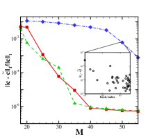
In our numerical experiments, we were able to recover $\bm{c}$ using fewer samples than the number $M$—as suggested by the sufficient condition (Theorem 2.5) originally given by Rauhut Rauhut_2012sparseLegen —since this number is based on the worst case scenario and is not, in general, a sharp bound. Figure 1(b) shows the numerical results of a test case with $\bm{c}_{T_{\bm{\alpha}}}=1$, $\bm{c}_{T_{\bm{\alpha}}^{c}}=0$, $|T_{\bm{\alpha}}|=5$. For each $M$, $200$ CS implementations were conducted to compute the average of the relative error $\|\bm{c}-\tilde{\bm{c}}\|_{1}/\|\bm{c}\|_{1}$. The exact and near-orthonormal amdP bases show similar performance, where $\bm{c}$ can be accurately recovered (up to $\|\bm{\varepsilon}\|_{2}$) using $M=45$ training points. In contrast, the Legendre basis yields larger relative error in $\ell_{1}$-norm. The relative error of the recovered coefficients from one CS implementation with Legendre basis is shown in the inset plot of Figure 1(b).

IV.1.2 Non-sparse linear systems

We also tested the recovery performance when the exact representation is not sparse. The vector $\bm{c}$ is chosen with a random non-zero index set $T_{\bm{\alpha}}$ with $|T_{\bm{\alpha}}|=120$. Individual components of $\bm{c}_{T_{\bm{\alpha}}}$ are i.i.d. log-normal, such that $\log\bm{c}_{T_{\bm{\alpha}}}\sim\mathcal{N}(0,2)$. For each size ($M$) of the training set, $200$ CS implementations were conducted to compute the average of the numerical error $\|\bm{c}-\tilde{\bm{c}}\|_{2}$, as shown in Figure 2(a). Similar to the previous example, the Legendre basis exhibits the largest approximation error. The near-orthonormal basis shows smaller error than the exact orthonormal basis.

Figure 2: The measurement matrices constructed by different bases show different numerical performance for the recovery of non-sparse vector. The near-orthonormal basis shows the most accurate result. (a) $l_{1}$ error of the recovered vector $\mathbf{c}$ with different bases. “ ”: the exact orthonormal amdP basis; “ ”: the near-orthonormal amdP basis; “ ”: Legendre basis. (b-d) Contours of $|\mathbf{c}_{\bm{\alpha}^{\prime}}-\tilde{\mathbf{c}}_{\bm{\alpha}^{\prime}}|$ (sorted by magnitude) from training sets of size $M=230$ with Legendre (top right), orthonormal (bottom left) and near-orthonormal bases (bottom right).

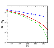
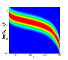
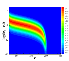
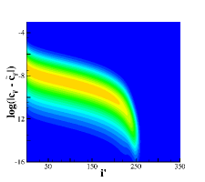
We also computed the density distribution of individual component $|\bm{c}_{i^{\prime}}-\tilde{\bm{c}}_{i^{\prime}}|$, where $i^{\prime}$ refers to single index sorted by the magnitude in descending order. Figure 2(b-d) shows that, compared with the exact orthonormal basis and the Legendre basis, the distribution of $\log\left|\bm{c}_{i^{\prime}}-\tilde{\bm{c}}_{i^{\prime}}\right|$ obtained from near-orthonormal basis is biased toward the smallest magnitudes for error of individual $i^{\prime}$. This result can be interpreted as that the average of $\|\bm{c}-\tilde{\bm{c}}\|_{2}$ of the near orthogonal basis is smaller than that of the exact orthogonal basis and also outperforms the Legendre basis.

IV.2 Systems with explicit knowledge of density function

In this subsection, we demonstrate the proposed method in systems with common non-Gaussian randomness with analytical density function $\omega(\bm{\xi})$. We show that the present method based on orthonormal basis construction and rotation of the random variables exploits the sparser representation of QoI while retaining proper orthogonality with respect to rotated variables. Therefore, it yields more accurate surrogate models than other approaches based on the direct recovery of $\bm{c}$ without the sparsity enhancement rotation procedure and/or directly applying the rotation procedure without reconstruction of the orthonormal amdP basis.

IV.2.1 High-dimensional polynomial

For the first numerical example, we consider a high-dimensional polynomial function

$$f(\bm{\xi})=\sum_{|\bm{\alpha}|\leq 3}\hat{c}_{\bm{\alpha}}\hat{\psi}_{\bm{\alpha}}(\bm{\xi})=\sum_{i=1}^{N}\frac{\eta_{i}}{|i|^{1.5}}\hat{\psi}_{i}(\bm{\xi}),$$ (IV.5)

where $\hat{\psi}_{\bm{\alpha}}$ and $\hat{\psi}_{i}$ represent monomial basis functions, $\eta_{i}$ represents uniform random variables $\mathcal{U}\left[0,1\right].$ We employed this polynomial function with sparse coefficients as a benchmark problem to examine the recovery accuracy of the present method. $\bm{\xi}$ is a random vector consisting of $20$ i.i.d. random variables. The density function of the $i\mathchar 45\relax$th variable $\xi_{i}$ is given by

$$\omega(\xi_{i})=e^{-\xi_{i}},$$ (IV.6)

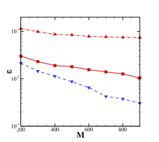
where the corresponding orthonormal basis are given by the Laguerre polynomials. Accordingly, we construct a 3-order polynomial expansion $\tilde{f}(\bm{\xi})$ with $N=1771$ multivariate basis functions, which are the tensor product of the univariate Laguerre polynomials. Figure 3 shows the relative $l_{2}$ error of $\tilde{f}$ computed by level $4$ sparse grid integration. Similar to the previous example, the probability density function (PDF) of $\bm{\chi}$ does not retain the form $\omega^{\prime}(\bm{\chi})=\prod_{i=1}^{d}\exp(-\chi_{i})$ after the rotation. Iteratively employing the multivariate Laguerre polynomials to represent $\tilde{g}(\bm{\chi})$ may result in erroneous prediction (the red dash-dotted curve). Alternatively, such a problem can be addressed by using the reconstructed orthonormal amdP basis with respect to $\bm{\chi}$, which yields a smaller error than $\tilde{f}(\bm{\xi})$ (the blue dashed curve).

Figure 3: Sparsity-enhancing rotation with the reconstructed orthonormal amdP basis yields the most accurate recovery of a high-dimensional polynomial function of random vectors following density function given by Equation (IV.6). Directly applying the rotation procedure without reconstructing the orthonormal basis yields errorneous prediction. “ ”: Laguerre polynomial basis with respect to $\bm{\xi}$; “ ”: Laguerre polynomial basis with respect to rotated vector $\bm{\chi}$; “ ”: the reconstructed amdP orthonormal basis with respect to rotated vector $\bm{\chi}$.

IV.2.2 One-dimensional elliptic PDEs with high-dimensional random inputs

We applied the proposed method to model the solution to a one-dimensional (1D) elliptic PDE with high dimensional random input

$$-\frac{d}{dx}\left(D(x;\bm{\xi})\frac{du(x;\bm{\xi})}{dx}\right)=1, \quad x\in(0,1)$$ (IV.7)

$$u(0)=u(1)=0,$$

where $a(x;\bm{\xi}):=\log D(x;\bm{\xi})$ is the stochastic input and $a(x;\bm{\xi})$ was a stationary process with correlation function

$$K(x,x^{\prime})=\exp\left(\dfrac{|x-x^{\prime}|}{l_{c}}\right),$$ (IV.8)

where $l_{c}$ is the correlation length. We constructed $a(x;\bm{\xi})$ by the Karhunen-Loève (KL) expansion:

$$a(x;\bm{\xi})=a_{0}(x)+\sigma\sum_{i=1}^{d}\sqrt{\lambda_{i}}\phi_{i}(x)\xi_{i},$$ (IV.9)

where $\{\lambda_{i}\}_{i=1}^{d}$, and $\{\phi_{i}(x)\}_{i=1}^{d}$ are the $d$ largest eigenvalues and the corresponding eigenfunctions of $K(x,x^{\prime})$. The values of $\lambda_{i}$ and the analytical expressions for $\phi_{i}$ were available from the literature JardakSK02 . The $\xi_{i}$ are i.i.d.  random variables on $\left[-1,1\right]$. The density function of $\xi_{i}$ is given by

$$\omega(\xi_{i})=\frac{1}{\pi\sqrt{1-\xi_{i}^{2}}},$$ (IV.10)

where the corresponding orthonormal basis consists of Chebyshev polynomials of the first kind. For this example, we set $a_{0}(x)\equiv 1$, $\sigma=0.8$, $l_{c}=0.14$ and $d=16$. We chose the quantity of interest as $u(x;\bm{\xi})$ at $x=0.45$ and constructed a 3-order polynomial expansion with $N=969$ basis functions. Figure 4 shows the relative $l_{2}$ error of the constructed $\tilde{f}(\bm{\xi})$ and $\tilde{g}({\bm{\chi}})$.

Figure 4: Sparsity-enhancing rotation with reconstructed orthonormal basis yield the most accurate surrogate models for a 1D elliptical PDE with random permeability coefficient modeled by Equations (IV.9) and (IV.10). Directly applying the rotation procedure without reconstructing the orthonormal basis yields increased numerical error. “ ”: Chebyshev polynomial basis with respect to $\bm{\xi}$; “ ”: Chebyshev polynomial basis with respect to rotated vector $\bm{\chi}$; “ ”: the reconstructed orthonormal amdP basis with respect to rotated vector $\bm{\chi}$.

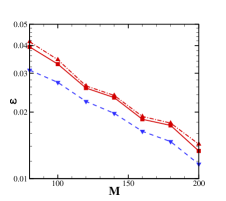
For the density function $\omega(\bm{\xi}_{i})$ given by (IV.10), $\tilde{f}(\bm{\xi})$ can be represented by a multivariate basis constructed by the tensor products of univariate Chebyshev polynomials. However, in general, the PDF of $\bm{\chi}$ does not retain the form $\omega^{\prime}(\bm{\chi})=\prod_{i=1}^{d}\frac{1}{\pi\sqrt{1-\chi_{i}^{2}}}$. As shown in Figure 4, iteratively employing the multivariate Chebyshev polynomials to represent $\tilde{g}(\bm{\chi})$ (the red dash-dotted curve)—as done in previous studies Yang_Wan_rotation_2017 —resulted in a larger error than $\tilde{f}(\bm{\xi}).$ Representing $\tilde{g}(\bm{\chi})$ by the reconstructed orthonormal amdP basis (the blue dashed curve) further decreases the numerical error compared to $\tilde{f}(\bm{\xi})$ (the solid red curve).

IV.3 Systems with implicit knowledge of density function

In this suite of benchmark examples, we investigated the applicability and efficiency of the developed DSRAR framework based on data-driven orthonormal bases construction and sparsity enhanced rotation.

IV.3.1 High-dimensional polynomials

We studied the ability of the data-driven method to recover a high-dimensional polynomial function

$$f(\bm{\xi})=\sum_{\bm{\alpha}\in T_{\bm{\alpha}}}\hat{\psi}_{\bm{\alpha}}(\bm{\xi}),$$ (IV.11)

where $\hat{\psi}_{\bm{\alpha}}$ represents the monomial basis function, $T_{\bm{\alpha}}$ represents a set containing $50$ indices randomly chosen from $\Lambda_{p}^{d}$ with $d=25$ and $p=3$. The sample set $S$ of random vector $\bm{\xi}$ for basis construction was generated from the Gaussian mixture model specified in (IV.1) with $|S|=2\times 10^{5}$.

We approximated $f(\bm{\xi})$ by a 3-order polynomial expansion $\tilde{f}(\bm{\xi})=\sum_{i=1}^{N}\tilde{c}_{i}\psi_{i}(\bm{\xi})$ with $N=3276$. Figure 5(a) shows the relative $l_{2}$ error of the constructed surrogate model $\tilde{f}$ defined by

$$\epsilon=\left(\int(f(\bm{\xi})-\tilde{f}(\bm{\xi}))^{2}\,\mathrm{d}\nu_{S_{2}}(\bm{\xi})\big{/}\int f(\bm{\xi})^{2}\,\mathrm{d}\nu_{S_{2}}(\bm{\xi})\right)^{\frac{1}{2}},$$ (IV.12)

where $20$ implementations were utilized for each training sample size number $M$.

Figure 5: Numerical results for recovery of a high-dimensional polynomial function. The combination of near-orthonormal basis construction with the sparsity enhancement rotation procedure yields the most accurate results. Directly applying the rotation procedure to the Legendre basis may lead to increased error despite increased sparsity in $\bm{c}$. (a) Relative $l_{2}$ error of the recovered polynomial function with different bases: the exact orthonormal amdP basis with respect to $\bm{\xi}$ (“ ”) and $\bm{\chi}$ (“ ”); the near-orthonormal amdP basis with respect to $\bm{\xi}$ (“ ”) and $\bm{\chi}$ (“ ”); Legendre basis with respect to $\bm{\xi}$ (“ ”) and $\bm{\chi}$( “ ”). (b) Coefficients magnitude $|c_{i}|$ recovered using different bases. “ ”: the exact orthonormal amdP basis with respect to $\bm{\xi}$; “ ”: the near-orthonormal amdP basis with respect to $\bm{\xi}$; “ ”: Legendre basis with respect to $\bm{\xi}$. (c) Recovered coefficient magnitude $|\mathbf{c}_{i}|$ using the near orthogonal basis with respect to $\bm{\xi}$ (“ ”) and $\bm{\chi}$ (“ ”). The dashed vertical lines indicate the separation between different polynomial orders $p$. (d) Recovered coefficient magnitude $|\mathbf{c}_{i}|$ using the Legendre basis with respect to $\bm{\xi}$ (“ ”) and $\bm{\chi}$ (“ ”).

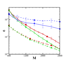
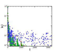
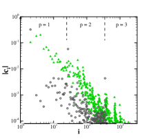
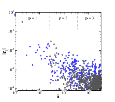
As shown in Figure 5(a), $\tilde{f}(\bm{\xi})$ constructed by the near-orthonormal amdP basis yielded the smallest error while the tensor product of Legendre basis functions yielded the largest error. Accordingly, the magnitudes of the recovered coefficients $|\tilde{c}_{i}|$ by the exact and near-orthonormal bases decayed more quickly than those recovered using the Legendre basis functions, as shown in Figure 5(b). Furthermore, $\tilde{f}(\bm{\xi})$ allowed us to define a new random vector $\bm{\chi}$, which further enhanced the sparsity of $\bm{c}$, as shown in Figures 5(c) and (d). Following Step 5 in Algorithm 4, we defined a new random $\bm{\chi}$ through rotation. The associated representation coefficient vector $\bm{c}$ has enhanced sparsity.

However, for the exact and near-orthonormal basis, the $\tilde{g}(\bm{\chi})$ gave smaller errors (the dashed curve) than $\tilde{f}(\bm{\xi})$ (the solid curve), as shown in Figure 5(a). Thus, enhancing the sparsity of $\bm{c}$ alone does not guarantee enhanced accuracy of $\tilde{f}$. In particular, $\tilde{g}(\bm{\chi})$ constructed by the Legendre basis yielded larger error than $\tilde{f}(\bm{\xi})$ as demonstrated in Figure 5(a); although, the sparsity of $\bm{c}$ was greater, as seen in Figure 5(d). This behavior indicates that retaining the orthonormal condition can be crucial for the accurate construction of $\tilde{f}$. The basis bound (see Table 2 in B) provides a metric to understand why the near-orthonormal basis performs better than the exact orthonormal basis.

IV.3.2 1D elliptic PDEs with high-dimensional random inputs

In this example, we revisited the 1D elliptic PDE (IV.7) with random coefficient given by Equation (IV.9). Here we set $a_{0}(x)\equiv 1$, $\sigma=1$, $l_{c}=0.12$ and $d=20$ such that $\sum_{i=1}^{d}\lambda_{i}>0.91\sum_{i=1}^{\infty}\lambda_{i}$.

Similar to the work by Zabaras et al. Zabaras_2014 , a non-Gaussian multivariate distribution was used for $\bm{\xi}=\left(\xi_{1},\xi_{2},\cdots,\xi_{d}\right)$. We generated a sample set $\left\{\tilde{\bm{\xi}}^{(k)}\right\}_{k=1}^{Ns}$, where $N_{s}=2\times 10^{5}$ and $\tilde{\bm{\xi}}$ came from the Gaussian mixture distribution specified in (IV.1). We used PCA to transform $\tilde{\bm{\xi}}$ to $\bm{\xi}$ such that $\mathbb{E}\left[\bm{\xi}_{i}\right]=0$ and $\mathbb{E}\left[\bm{\xi}_{i}\bm{\xi}_{j}\right]=\delta_{ij}$. For each input sample $\bm{\xi}^{(k)}$, $a$ and $u$ only depended on $x$ and the solution of the deterministic elliptic equation is given by Yang_2013reweightedL1

$$\begin{split}&u(x)=u(0)+\int_{0}^{x}\dfrac{a(0)u(0)^{\prime}-y}{a(y)}\,\mathrm{d}y\\ &a(0)u(0)^{\prime}=\left(\int_{0}^{1}\dfrac{y}{a(y)}\,\mathrm{d}y\right)\Big{/}\left(\int_{0}^{1}\dfrac{1}{a(y)}\,\mathrm{d}y\right).\end{split}$$ (IV.13)

We chose the QoI to be $u(x;\bm{\xi})$ at $x=0.35$ and constructed a 3-order polynomial expansion with $N=1771$ basis functions. Figure 6 shows the relative $l_{2}$ error of $\tilde{f}(\bm{\xi})$ (solid curve) and $\tilde{g}(\bm{\chi})$ (dashed curve) constructed by different bases.

Figure 6: The combination of near-orthonormal basis construction and sparsity enhancement rotation yields the most accurate results, as shown through the relative $l_{2}$ error of the constructed surrogate model for the 1D elliptic PDE with random permeability coefficient: the exact orthonormal amdP basis with respect to $\bm{\xi}$ (“ ”) and $\bm{\chi}$ (“ ”); Legendre basis with respect to $\bm{\xi}$ (“ ”) and $\bm{\chi}$( “ ”); Hermite basis with respect to $\bm{\xi}$ (“ ”); the near-orthonormal amdP basis with respect to $\bm{\chi}$ (“ ”).

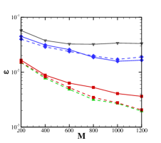
The data-driven bases (both exact orthonormal basis and near-orthonormal basis) showed more accurate results than the Legendre basis and the Hermite basis. In particular, the near-orthonormal basis with respect to the rotated variable $\bm{\chi}$ yielded the most accurate result (the green dashed curve). In contrast, directly employing the Legendre basis to the rotated variable $\bm{\chi}$ without reconstructing the basis function led to increased $l_{2}$ error, although $\bm{c}$ shows more sparsity in terms of $\bm{\chi}$ (the gray dashed curve) than $\bm{\xi}$ (the gray solid curve).

IV.4 UQ study of a molecule system under Non-Gaussian conformational distributions

We demonstrated the proposed method on a physical system exploring conformational uncertainty in a small molecule system. Molecular properties, such as solvation energies or solvent-accessible surface areas, are often calculated using single molecular conformations. However, due to thermal energy, a molecule undergoes conformational fluctuations which can induce significant uncertainty in properties calculated from single structures. Our previous work Lei_Yang_MMS_2015 was focused on quantifying this uncertainty using a simple multivariate Gaussian model for conformational fluctuations: the elastic network model Ati_Bahar_BJ_2001 . However, it is well known that the conformational fluctuations are often non-Gaussian due to the complicated structure of the underlying energy landscape. Therefore, in the current study, we construct the data-driven basis directly from the samples of molecular trajectories collected from molecular dynamics (MD) simulations, thus eliminating the over-simplified Gaussian assumption.

We simulated the dynamics of the small molecule benzyl bromide under equilibrium (see E for details) and collected a sample set of the instantaneous molecular structure $\left\{\mathbf{r}^{(k)}\right\}_{k=1}^{N_{s}}$ from MD simulation trajectories over $20\mu$s. In what follows, $N_{s}=2\times 10^{5}$ and $\mathbf{r}$ represent the positions of individual atoms. As a pre-processing step, we transformed $\left\{\mathbf{r}^{(k)}\right\}_{k=1}^{N_{s}}$ into a set of uncorrelated random vectors $S=\left\{\mathbf{\bm{\xi}}^{(k)}\right\}_{k=1}^{N_{s}}$ via PCA:

$$\begin{split}&\bm{\Sigma}=\mathbb{E}\left[\left(\mathbf{r}-\bar{\mathbf{r}}\right)\left(\mathbf{r}-\bar{\mathbf{r}}\right)^{T}\right]\\ &\bm{\Sigma}=\mathbf{Q}\bm{\Gamma}\mathbf{Q}^{T}\quad\bm{\xi}=\bm{\Gamma}^{-1/2}\mathbf{Q}^{T}\mathbf{r},\end{split}$$ (IV.14)

where the average $\mathbb{E}[\cdot]$ is taken over the entire sample set and $\bm{\xi}\in\mathbb{R}^{12}$ is the normalized random vector that represents $99.99\%$ of the observed variance. Figures 7(a) and (b) show the joint distributions of $\left(\xi_{1},\xi_{2}\right)$ and $\left(\xi_{1},\xi_{3}\right)$.

Figure 7: The present method based on data-driven basis construction and sparsity enhancement rotation yields the most accurate surrogate model for molecular systems with mutually dependent non-Gaussian density distributions. (a-b) Sampling points representing the joint distributions $\left(\xi_{1},\xi_{2}\right)$ (left) and $\left(\xi_{1},\xi_{3}\right)$ (right). (c-d) Relative $l_{2}$ error of the polar solvation energy (left) and the local SASA (right) of an individual atom (the H9 atom attached to the ortho-carbon atom) obtained with different numbers of training data $M$: the exact amdP orthonormal basis with respect to $\bm{\xi}$ (“ ”) and $\bm{\chi}$ (“ ”); Hermite basis with respect to $\bm{\xi}$ (“ ”) and $\bm{\chi}$ (“ ”); Legendre basis with respect to $\bm{\xi}$ (“ ”); the near-orthonormal amdP basis with respect to $\bm{\chi}$ (“ ”).

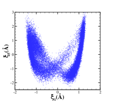
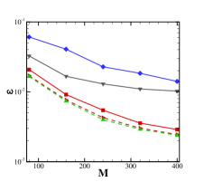
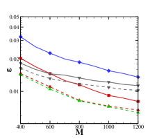
Although the individual components of $\bm{\xi}$ are uncorrelated, the joint density distributions are mutually dependent and deviate from the standard Gaussian distributions.

We chose the polar solvation energy and SASA as the target QoIs for this system. The polar solvation energy was modeled by the Poisson-Boltzmann equation ren_biomolecular_2012 ; baker_biomolecular_2005

$$-\nabla\cdot(\epsilon_{f}(\bm{x};\bm{\xi})\nabla\varphi(\bm{x};\bm{\xi}))=\rho_{f}(\bm{x};\bm{\xi})$$ (IV.15)

which relates the electrostatic potential $\varphi$ to a dielectric coefficient $\epsilon_{f}$ and a fixed charge distribution $\rho_{f}$. Equation (IV.15) is typically solved with Dirichlet boundary conditions set to an analytical asymptotic solution of the equation for an infinite domain. The dielectric coefficient $\epsilon_{f}$ implicitly represents the boundary between the atoms of the molecule and the surrounding solvent: the coefficient changes rapidly across this boundary from a low dielectric value in the molecular interior to a high dielectric value in the solvent. The charge distribution $\rho_{f}$ is generally modeled as a collection of $\delta$-like functions centered on the atoms of the molecule with magnitudes proportional to the atomic partial charges. Both $\epsilon_{f}$ and $\rho_{f}$ are dependent on the instantaneous molecular structure (i.e., $\bm{\xi}$). The polar solvation energy was calculated from

$$G_{p}(\bm{\xi})=\int\rho_{f}(\bm{x};\bm{\xi})\left(\varphi(\bm{x};\bm{\xi})-\varphi_{h}(\bm{x};\bm{\xi})\right)d\bm{x}$$ (IV.16)

where $\varphi_{h}$ is a reference potential obtained from solution of

$$-\epsilon_{h}\nabla^{2}\varphi_{h}(\bm{x};\bm{\xi})=\rho_{f}(\bm{x};\bm{\xi})$$ (IV.17)

where $\epsilon_{h}$ is a constant reference dielectric value. We used the Adaptive Poisson-Boltzmann Solver (APBS) software to solve the equations above APBS_2018 . Besides the solvation energy of the whole molecule, we also studied a local property like the SASA of an individual atom (the H9 atom attached to the ortho-carbon atom of the benzyl bromide molecule, see Figure 11) by the Shrake-Rupley algorithm Shrake_JMB_1973 using APBS. Details of the APBS calculations are presented in E.

Figures 7(c) and (d) show the relative $l_{2}$ error of the constructed surrogate model $\tilde{f}(\bm{\xi})$ for the solvation energy and SASA using a 4-order gPC expansion with $N=1820$ basis functions. For both QoIs, the near-orthonormal and orthonormal bases with respect to the rotated variable $\bm{\chi}$ (dashed curves) yield similar error which is much smaller than the error of Legendre and Hermite bases. A possible explanation for the similar performance of the near-orthonormal and orthonormal bases is the closeness of the basis bound estimates for these two bases (see Table 3 in B).

Figure 8: The present method yields the most accurate prediction on the PDF of the QoI for the molecular systems. Direct fitting of the underlying density $\omega(\bm{\xi})$ using Gaussian Mixture model may induce biased error to the PDF prediction. (a) Fitted random variables $(\xi_{1},\xi_{2})$ with Gaussian mixture models. (b) PDF of the solvation energy obtained with the Gaussian Mixture model and the present data-driven approach. “ ”: reference solution obtained from $2\times 10^{5}$ MC samples; “ ”: direct MC sampling using the same set of $200$ samples; “ ”: present method using the same set of $200$ samples; “ ”: fitting Gaussian Mixture model using $800$ samples.

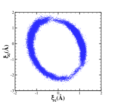
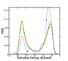
Instead of the direct construction of $\tilde{f}(\bm{\xi})$ using data-driven basis functions, another possible approach to characterize the uncertainty of the molecular system is to fit the distribution density $\omega(\bm{\xi})$ with a distribution model such as a Gaussian Mixture model. Figure 8 (a) shows a scatter plot of the joint distribution $\left(\xi_{1},\xi_{2}\right)$ extracted from the fitted Gaussian mixture distribution $\tilde{\omega}(\bm{\xi})$ using $7$ Gaussian modes. Accordingly, we can construct the surrogate model for each Gaussian mode using standard Hermite basis function. However, it is well-known that accurate construction of $\omega(\bm{\xi})$ is a numerically challenging problem for $d>4$. As shown in Figure 8(b), direct fitting $\omega(\bm{\xi})$ by $\tilde{\omega}(\bm{\xi})$ induces non-negligible error and leads to biased prediction of the PDF of the solvation energy. Furthermore, we lose the one-to-one mapping between the individual conformation state $\bm{\xi}$ and the QoIs through the constructed surrogate model $\tilde{f}(\bm{\xi})$.

V Summary

In this study, we have developed a DSRAR framework for constructing surrogate models irrespective of the mutual dependence between the components of random inputs using limited training points. To the best of our knowledge, this problem has not been addressed by previous UQ studies based on polynomial chaos expansions. The DSRAR framework does not assume mutual independence between the components of random inputs and therefore can be applied to UQ in complex systems where information about the underlying random distribution can be implicit. To construct the surrogate model, this framework uses data-driven amdP basis construction and a sparsity-enhancing rotation procedure which leads to more accurate recovery of the sparse representation of the target function. The method benefits from both the orthonormal basis expansion and the enhanced sparsity of the expansion coefficients. With the assumption that there exists a sparse representation of the surrogate model, the DSRAR approach can be applied to challenging UQ problems under two widely encountered situations: (I) probability measure implicitly represented by a large collection of samples and (II) non-Gaussian probability measures with explicit (analytical) forms. For systems with explicit knowledge of the probability measure, our method exploits sparser representations of QoIs while retaining proper orthogonality with respect to rotated variables. For systems with randomness implicitly represented by a large collection of random samples, we also proposed a heuristic method to construct a near-orthonormal basis in addition to the exact orthonormal basis with respect to the discrete measure. The near-orthonormal basis shows a smaller basis bound and empirically yields more accurate representations. The numerical examples show the effectiveness of our method for realistic problems on quantifying uncertainty propagation in molecular system under conformational fluctuations as well as PDEs with arbitrary underlying probability measures.

For future study, we note that several issues not considered in the present work could further improve the performance of the present DSRAR framework. The heuristic approach to constructing near-orthonormal basis introduced in this study yields smaller basis bounds and more accurate representations than existing methods. However, we do not have the theoretical analysis to formally show that the near-orthonormal basis is optimal and to establish the conditions under which it outperforms the exact orthonormal basis. It would be interesting to investigate different approaches of data-driven basis construction to further improve the properties of measurement matrix for CS purposes. For instance, if new data becomes available after the surrogate construction, it is worth exploring how to use the new information to design more sophisticated (cross-validation) strategies to optimize the orthonormal threshold values and the basis construction procedure. Furthermore, our study used a standard $\ell_{1}$ minimization approach for relaxing the CS problem and recovering a sparse solution of the under-determined system. However, other optimization approaches can be employed when the measurement matrix is highly coherent when $\ell_{1}$ minimization is not necessarily optimal. Finally, it would be interesting to employ the developed DSRAR approach for UQ study in other complex biological systems Bajaj_ACM_2016 ; Bajaj_JCB_2018 . Such results will be presented in a future publication.

Appendix A The proof of Theorem  IV.4

Proof.

Let $\bm{v}\in\rm{Ker}~{}\bm{A}$ and $\bm{x}\neq\bm{c}$ another solution of $\bm{A}\bm{x}=\bm{b}$. To show that $\bm{c}$ is the unique $l_{1}$ minimizer of $\bm{A}\bm{c}=\bm{b}$, it is sufficient if

$$\|\bm{v}_{T_{\bm{\alpha}}}\|_{1}<\|\bm{v}_{T_{\bm{\alpha}}^{c}}\|_{1},$$ (A.1)

which gives

$$\begin{split}\|\bm{c}\|_{1}&\leq\|\bm{c}-\bm{x}_{T_{\bm{\alpha}}}\|_{1}+\|\bm{x}_{T_{\bm{\alpha}}}\|_{1}=\|\bm{c}_{T_{\bm{\alpha}}}-\bm{x}_{T_{\bm{\alpha}}}\|_{1}+\|\bm{x}_{T_{\bm{\alpha}}}\|_{1}=\|\bm{v}_{T_{\bm{\alpha}}}\|_{1}+\|\bm{x}_{T_{\bm{\alpha}}}\|_{1}\\ &<\|\bm{v}_{T_{\bm{\alpha}}^{c}}\|_{1}+\|\bm{x}_{T_{\bm{\alpha}}}\|_{1}=\|\bm{x}\|_{1}.\end{split}$$ (A.2)

To satisfy (A.1), we partition $T_{\bm{\alpha}}^{c}$ into $T_{\bm{\alpha}}^{c}=T_{\bm{\alpha},1}^{c}\bigcup T_{\bm{\alpha},2}^{c}\bigcup\cdots$, where $T_{\bm{\alpha},1}^{c}$ is the index set of $s$ largest absolute entries of $\bm{v}$ in $T_{\bm{\alpha}}^{c}$, $T_{\bm{\alpha},2}^{c}$ is the index set of $s$ largest absolute entries of $\bm{v}$ in $T_{\bm{\alpha}}^{c}T_{\bm{\alpha},1}^{c}$. Accordingly,

$$\|\bm{v}_{T_{\bm{\alpha}}}\|_{2}^{2}\leq\frac{1}{1-\delta_{s}}\|\bm{A}\bm{v}_{T_{\bm{\alpha}}}\|_{2}=\frac{1}{1-\delta_{s}}\sum_{k=1}\left\langle\bm{A}\bm{v}_{T_{\bm{\alpha}}},\bm{A}(-\bm{v}_{T_{\bm{\alpha},k}^{c}})\right\rangle\leq\frac{\theta_{s}}{1-\delta_{s}}\sum_{k=1}\|\bm{v}_{T_{\bm{\alpha}}}\|_{2}\|\bm{v}_{T_{\bm{\alpha},k}^{c}}\|_{2},$$ (A.3)

which gives $\|\bm{v}_{T_{\bm{\alpha}}}\|_{2}\leq\frac{\theta_{s}}{1-\delta_{s}}\sum_{k=1}\|\bm{v}_{T_{\bm{\alpha},k}^{c}}\|_{2}$. The remaining of the proof is straightforward and follows Theorem 2.6 of Rauhut Rauhut_2010CsSM . By the Cauchy-Schwarz inequality, we obtain

$$\|\bm{v}_{T_{\bm{\alpha}}}\|_{1}\leq\frac{\theta_{s}}{1-\delta_{s}}\left(\|\bm{v}_{T_{\bm{\alpha}}}\|_{1}+\|\bm{v}_{T_{\bm{\alpha}}^{c}}\|_{1}\right).$$ (A.4)

Equation (A.1) follows if $\frac{\theta_{s}}{1-\delta_{s}}<0.5$. ∎

Remark A.1.

We emphasize that Theorem IV.4 holds only for the given index set $T_{\bm{\alpha}}$; it provides a metric to examine the recovery accuracy with respect to measurement matrix $\bm{A}$ and should not be viewed as the sufficient condition for exact recovery of arbitrary $s$-sparse vector via $l_{1}$-minimization (see canonical references Candes_2005Decoding ; Candes_2006Stablesrec ; Rauhut_2010CsSM for details). Theorem IV.4 also indicates that, for the given index set $T_{\bm{\alpha}}$, small $\|\bm{A}^{*}_{T_{\bm{\alpha}}}\bm{A}_{T_{\bm{\alpha}}}-I\|_{2}$ will promote the recover of $\bm{v}_{T_{\bm{\alpha}}}$.

Appendix B Measurement matrix and basis bounds

B.1 Null space of measurement matrix from Section IV.1

Let $\tilde{\bm{c}}=\bm{c}+\bm{v}$, $\bm{v}\in\textrm{Ker}~{}\bm{A}$ where $\bm{A}$ is the measurement matrix defined in (IV.3). From the null space property Rauhut_2010CsSM , $\tilde{\bm{c}}$ does not fully recover $\bm{c}$ by $\ell_{1}$ minimization (i.e., equation (II.6)) only if $\|\tilde{\bm{c}}\|_{1}<\|\bm{c}\|_{1}$. As a necessary condition for the failure of recovery, it requires

$$\left\|\bm{v}_{T_{\bm{\alpha}}}\right\|_{1}>\left\|\bm{v}_{T_{\bm{\alpha}}^{c}}\right\|_{1},$$ (B.1)

where $T_{\bm{\alpha}}^{c}$ refers to the complement of $T_{\bm{\alpha}}$. Accordingly, different null space of measurement matrix $\bm{A}$ generally leads to different recovery error.

We examined the above necessary condition (B.1) for different measurement matrices by randomly choosing a non-zero index set $T_{\bm{\alpha}}$ with $\left|T_{\bm{\alpha}}\right|=50$ and $M=180$. For $\bm{A}$ constructed by both basis sets, we collected $1000$ normalized $\bm{v}\in\rm{Ker}~{}\bm{A}$ that satisfy $\left\|\bm{v}_{T_{\bm{\alpha}}}\right\|_{1}>\left\|\bm{v}_{T_{\bm{\alpha}}^{c}}\right\|_{1}$. Figure 9 shows the density contour of individual component $\left|\bm{v}_{i^{\prime}}\right|$ in log-scale, where $i^{\prime}$ refers to the index sorted by magnitude in descending order.

Figure 9: The null spaces of measurement matrices constructed by the exact and near-orthonormal bases are different under $\left\|\bm{v}_{T_{\bm{\alpha}}}\right\|_{1}>\left\|\bm{v}_{T_{\bm{\alpha}}^{c}}\right\|_{1}$—a necessary condition for $\bm{c}$ not being recoverable exactly. Density contour of the normalized null space vector component $\log|\rm{v}_{i^{\prime}}|$ (sorted by magnitude) of the measurement matrix $\bm{A}$ constructed by orthogonal (a) and near-orthogonal basis functions (b) that satisfy $\left\|\bm{v}_{T_{\bm{\alpha}}}\right\|_{1}>\left\|\bm{v}_{T_{\bm{\alpha}}^{c}}\right\|_{1}$ and $\|\bm{v}\|_{2}=1$.

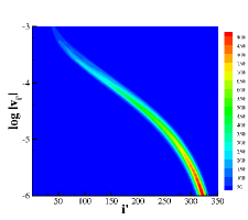
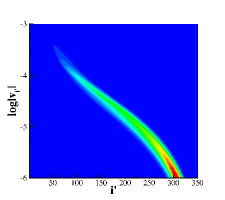
The two basis sets demonstrate different distributions of $\log\left|\bm{v}_{i^{\prime}}\right|$, which likely contribute to the different recovery errors shown in Figure 2.

B.2 Basis bounds

The lower bound of the required number of samples $M$ given in Theorem  II.5 suggests that bases with smaller basis bounds $K$ are preferred. We expect that smaller basis bounds will correlate with higher accuracy representations. For the constructed basis set $\psi_{i}(\bm{\xi}),i=1,\cdots,N$, we define the basis bound $\tilde{K}$ on the given data set $S$ by

$$\tilde{K}:=\frac{1}{|S_{M_{\sigma}}|}\sum_{\bm{\xi}\in S_{M_{\sigma}}}|k(\bm{\xi})|,$$ (B.2)

where the set $S_{M_{\sigma}}$ is defined by $S_{M_{\sigma}}=\left\{\bm{\xi}\Big{|}|k(\bm{\xi})-\mathbb{E}\left[k\right]|>M_{\sigma}\sigma\left[k\right],\bm{\xi}\in S\right\}$. Here $\displaystyle k(\bm{\xi}):=\mathop{\max}_{i}|\psi_{i}(\bm{\xi})|$ denotes the maximum magnitude for an individual sampling point $\bm{\xi}$, $\mathbb{E}\left[k\right]$ and $\sigma\left[k\right]$ represent the mean and the standard deviation of $k(\bm{\xi})$ on $S$ with respect to the discrete measure $\nu_{S}$. In this study, we present $\tilde{K}$ as an indication of the difference between the exact and near-orthonormal basis function. In compressive sensing, the measurement matrix only consists of limited number of samples. Therefore, we employ the mean of the tails in the basis bounds as an indicator of the upper bound of the largest entry values from the measurement matrix. $M_{\sigma}$ defines the range of this tail set. We choose $M_{\sigma}=5$ if not specified otherwise.

Table 1: $\tilde{K}$ of constructed basis set for Gaussian mixture system $d=25$, $p=2$ and $N_{s}=1\times 10^{5}$.

$M_{\sigma}$	$3$	$4$	$5$	$6$	$\displaystyle\mathop{\max}_{\bm{\xi}\in S}k(\bm{\xi})$
$\tilde{K}_{\rm orth}$	10.359	12.048	13.895	15.513	22.208
$\tilde{K}_{\rm near-orth}$	9.622	11.196	12.867	14.448	18.790

Following the definition by Equation (B.2), we examine the basis bound $\tilde{K}$ of the numerical examples presented in this study. Table 1 shows the results of Gaussian mixture system $\left\{\bm{\xi}^{(i)}\right\},i=1,\cdots,N_{s}$ with $N_{s}=1\times 10^{5}$, $d=25$ and $p=2$ which is defined in Section IV.1. For different values of $M_{\sigma}$, $\tilde{K}$ of the near orthogonal basis shows consistently smaller values than the values of the exact orthogonal basis set.

Table 2 shows the basis bound $\tilde{K}$ of the Gaussian mixture system which is studied in Section IV.3.1 with $N_{s}=2\times 10^{5}$, $d=25$ and $p=3$ . The values of $\tilde{K}$ for the near orthogonal basis are consistently smaller than the value for the exact orthogonal basis set no matter on the original random sample set or the rotated sample set. Furthermore, we present the basis bounds on the rotated sampling set $\left\{\bm{\chi}_{M}^{\left(i\right)}\right\}_{i=1}^{N_{s}}$, where the subscript “$M$” refers to the different number of training points utilized to construct the surrogate model $X(\bm{\xi})$. The near-orthogonal basis yields smaller $\tilde{K}$ than the exact orthogonal basis in each case.

Similarly, Table 3 shows $\tilde{K}$ of the constructed basis for uncertainty quantification of the molecular solvation energy ($d=12$, $p=4$ and $N_{s}=2\times 10^{5}$), which is studied in Section IV.4. The near-orthogonal basis yields smaller values consistently for different number ($\bm{\chi}_{M}$) of training points.

Table 2: $\tilde{K}$ of constructed basis set for Gaussian mixture system $d=25$, $p=3$ and $N_{s}=2\times 10^{5}$.

	$\bm{\xi}$	$\bm{\chi}_{M=400}$	$\bm{\chi}_{M=1200}$	$\bm{\chi}_{M=1600}$	$\bm{\chi}_{M=2400}$
$\tilde{K}_{\rm orth}$	32.497	32.522	32.079	33.142	32.308
$\tilde{K}_{\rm near-orth}$	28.320	29.811	29.407	29.512	29.192

Table 3: $\tilde{K}$ of constructed basis set for molecular system $d=12$, $p=4$ and $N_{s}=2\times 10^{5}$.

	$\bm{\chi}_{M=80}$	$\bm{\chi}_{M=160}$	$\bm{\chi}_{M=240}$	$\bm{\chi}_{M=320}$	$\bm{\chi}_{M=400}$
$\tilde{K}_{\rm orth}$	40.596	39.914	39.789	39.218	39.142
$\tilde{K}_{\rm near-orth}$	39.970	39.278	39.290	38.528	38.631

Appendix C Other metrics of surrogate model

Besides the relative $l_{2}$ error, we have also computed the predictivity coefficients $Q_{2}$ for the test cases of Gaussian Mixture systems (with $d=25$ and $p=3$) and the molecular systems. Similar to Ref. Marrel_Q2_2009 , $Q_{2}$ is defined by

$$Q_{2}=1-\int(f(\bm{\xi})-\tilde{f}(\bm{\xi}))^{2}\,\mathrm{d}\nu_{S_{2}}(\bm{\xi})\big{/}\int\left(f(\bm{\xi})-\bar{f}\right)^{2}\,\mathrm{d}\nu_{S_{2}}(\bm{\xi}),$$ (C.1)

where $\bar{f}$ represents the mean of QoI on $S_{2}$. The results are listed in Tab. 4, where the surrogate models are constructed by the present data-driven basis approach.

Table 4: The predictivity coefficient $Q_{2}$ for polynomial function with Gaussian Mixture measure ($d=25$ and $p=3$) and the molecular system for solvation energy and SASA of atom $\rm{H9}$.

molecule solvation	$M$	80	160	240	320	400
	$Q_{2}$	0.995715	0.999132	0.999731	0.999864	0.999911
molecule SASA	$M$	200	300	400	500	600
	$Q_{2}$	0.988675	0.996069	0.998272	0.998709	0.999027
Gaussian Mixture	$M$	200	300	400	500	600
	$Q_{2}$	0.998372	0.999347	0.999844	0.999892	0.999941

With the constructed surrogate model, we can further compute the Sobol’ sensitivity indices for QoI with dependent random variables. In brief, $f(\bm{\xi})$ is expanded by

$$f(\bm{\xi})=\eta_{0}(\bm{\xi})+\sum_{\bm{\beta}\in\Theta^{d}}\eta_{\bm{\beta}}(\bm{\xi}),$$ (C.2)

where $\Theta^{d}$ represents the collection of all subsets of $[1~{}:~{}d]$ and $\eta_{\bm{\beta}}(\bm{\xi})$ satisfies $\mathbb{E}\left[\eta_{\bm{\alpha}},\eta_{\bm{\beta}}\right]=0$, if $\bm{\alpha}\subset\bm{\beta}$. The sensitivity index $S_{\bm{\beta}}$ is given by

$$S_{\bm{\beta}}=\frac{\mathbb{V}(\eta_{\bm{\beta}})+\sum_{\bm{\alpha}\cap\bm{\beta}\neq\bm{\alpha},\bm{\beta}}\rm{Cov}(\eta_{\bm{\alpha}},\beta_{\bm{\beta}})}{\mathbb{V}(f)}$$ (C.3)

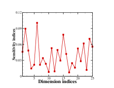
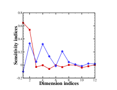
where $\mathbb{V}(\cdot)$ refers to the variance on $\nu_{S}$. We refer to Ref. Chastaing_sobol_2014 for the details. Fig. 4 shows the first order sensitivity indices for the test cases of Gaussian Mixture systems ($d=25$, $p=3$) and the biomolecular systems, where the surrogate models are constructed by the present data-driven basis approach using $M=800$, $M=240$ and $M=600$ training points, respectively. Based on the analysis, it is shown the dominant components are on the dimensions $(1,2,3,6,11,13,14,15,16,20,22,24,25)$, $(1,2,5)$ and $(1,2,4,5,7)$ ($90\%$ of total variance).

Figure 10: The first-order Sobol’ sensitivity indices for (a) polynomial function with Gaussian Mixture mesure ($d=25$, $p=3$) (b) molecular system for solvation energy (“ ”) and SASA of atom $\rm{H9}$(“ ”).

Appendix D Generation of Gaussian Mixture data set

We employ Matlab to generate the Gaussian Mixture data set in Sec. IV.1 by calling the function gmdistribution($\bm{\mu}$, $\left\{\Sigma_{i}\right\}_{i=1}^{3}$, $\bm{a}$). Here $\bm{a}=(0.5358,0.1281,0.3361)$. $\bm{\mu}$ is a $25\times 3$ random matrix with i.i.d. entries on $U[-2.5,2.5]$. $\left\{\Sigma_{i}\right\}_{i=1}^{3}$ is a $25\times 25\times 3$ array where $\Sigma_{i}$ is defined by

$$\bm{\Sigma}_{i}=(\bm{\Upsilon}_{i}{\bm{\Upsilon}_{i}}^{T}+\mathbf{I})/4,$$ (D.1)

where $\bm{\Upsilon}_{i}$ is a random matrix with i.i.d. entries from $\mathcal{U}[0,1]$ for $i=1,2,3$. $\bm{\mu}$ and $\Upsilon_{i}$ are generated by calling Matlab function rand() consequently with random number seed $200$.

Appendix E Molecular Dynamics simulation and calculation details

We performed all-atom MD simulation of benzyl bromide in water using GROMACS 5.1.2 GROMACS . The simulation system included a benzyl bromide molecule (see Figure 11 for the molecule structure) and 1011 water molecules. The General AMBER Force Field (GAFF) RN1 was used for benzyl bromide parameters. The partial charges of benzyl bromide molecule were calculated by RESP method RN2 . Bond lengths of benzyl bromide were constrained using the LINCS algorithm RN3 . The water molecule was modeled with the rigid TIP3P water model RN4 . The bond lengths and angles were held constant through the SETTLE algorithm RN5 . The system was equilibrated in the isothermal-isobaric ensemble for 10 ns at 300K and 1 bar after energy minimization. The van der Waals cut-off radii was 1.0 nm. Long-range electrostatics were calculated using a Particle Mesh Ewald (PME) summation with grid spacing of 0.12 nm. The time step was 2 fs. Isobaric-isothermal simulations were equilibrated using a V-rescale thermostat and Berendsen barostat. Following equilibration, the simulation was run for a production period of 20 $\mu$s in a NVT ensemble with a Nosé-Hoover thermostat. The trajectory was stored every 10000 time steps.

Figure 11: Sketch of the molecule benzyl bromide with labeled atoms.

APBS calculations BakerSJHM01 ; APBS_2018 were performed with $129^{3}$ grid points over a $40\times 40\times 40$ ų coarse grid domain with focusing to a $14\times 14\times 14$ ų fine grid domain with the grid origin located at the geometric center of the molecule. The Poisson equation was solved with Dirichlet boundary conditions based on the asymptotic behavior of multiple point charges in a homogeneous dielectric medium. The dielectric coefficient inside the domain used a van der Waals molecular volume definition with a dielectric value of 2.0 inside the molecule and 78.0 outside the molecule. Charges were modeled by Dirac delta functions but discretized to the finite difference grid points using a cubic spline approximation.