On the angular distribution of $\Lambda_{b}\to\Lambda(\to N\pi)\tau^{+}\tau^{-}$ decay

Abstract

We present a full angular distribution of the four body $\Lambda_{b}\to\Lambda(\to N\pi)\ell^{+}\ell^{-}$ decay where the leptons are massive and the $\Lambda_{b}$ is unpolarized, in an operator basis which includes the Standard Model operators, new vector and axial-vector operators, and scalar and pseudo-scalar operators. The angular coefficients are expressed in terms of transversity amplitudes. We study several $\Lambda_{b}\to\Lambda(\to p\pi)\tau^{+}\tau^{-}$ observables in the Standard Model and in the presence of the new operators. For our numerical analysis, we use the form factors from lattice QCD calculations.

1 Introduction

The loop induced rare $b\to s\ell^{+}\ell^{-}$ transitions are well known for their high sensitivity to physics beyond the Standard Model (SM), also known as new physics (NP). The $b\to s\ell^{+}\ell^{-}$ mediated decay of $B$ meson, the $B\to K^{\ast}(\to K\pi)\ell^{+}\ell^{-}$, is a very important decay mode in this regard as its full angular distribution gives access to a multitude of observables Kruger:1999xa that can uniquely test the SM. Therefore, the $B\to K^{\ast}(\to K\pi)\ell^{+}\ell^{-}$ decay is the topic of intense theoretical and experimental scrutiny in the past several decades. Recently, the LHCb measured Aaij:2015xza the first $b\to s\mu^{+}\mu^{-}$ mediated baryonic decay $\Lambda_{b}\to\Lambda\mu^{+}\mu^{-}$ which was earlier observed by the CDF Aaltonen:2011qs . The full angular distribution of $\Lambda_{b}\to\Lambda(\to N\pi)\mu^{+}\mu^{-}$ ($N\pi\equiv\{p^{+}\pi^{-},n^{0}\pi^{0}\}$) with unpolarized $\Lambda_{b}$ also provides a large number of observables Boer:2014kda which makes it at par with the $B\to K^{\ast}(\to K\pi)\ell^{+}\ell^{-}$ as far the number of accessible observables is concerned. On the other hand, if the polarization of the $\Lambda_{b}$ is accounted for, the number of observables that one can gain access to become more than three times than the unpolarized case Blake:2017une making this decay an unique test ground for the SM and searches for NP.

While the short-distance physics of $\Lambda_{b}\to\Lambda(\to N\pi)\ell^{+}\ell^{-}$, encoded in the $b\to s\ell^{+}\ell^{-}$ Wilson coefficients are very precisely known for some time Bobeth:1999mk , progress in the long distance calculations has recently been made. This includes the QCD sum-rules analysis of spectator-scattering corrections to the form factor relations Feldmann:2011xf , and better theoretical understanding of light-cone distribution amplitudes of $\Lambda_{b}$ baryon Ali:2012pn ; Bell:2013tfa ; Braun:2014npa . At low dilepton invariant mass squared $q^{2}$ or large recoil, the form factors are calculated in the light-cone sum rules in Refs. Wang:2008sm ; Wang:2015ndk , and in soft-collinear effective theory in Refs. Wang:2011uv ; Mannel:2011xg . The form factors have also been calculated in the relativistic quark model in Ref. Faustov:2017wbh . For our need of the form factors at large $q^{2}$ or low recoil, we use the results from the calculations in lattice QCD Detmold:2016pkz ; Detmold:2012vy

In a recent paper Das:2018sms we presented a model independent NP analysis of $\Lambda_{b}\to\Lambda\ell^{+}\ell^{-}$ decay where the NP operators include new vector and axial vector (VA) operators, scalar and pseudo-scalar (SP) operators, and tensor operators. In this analysis the mass of the final state leptons was neglected considering di-muon in the final state. The lepton mass should however be incorporated if there are $\tau^{+}\tau^{-}$ in the final state, or one wants to study lepton flavor universality (LFU) violation. Recent SM analysis of $\Lambda_{b}\to\Lambda(\to N\pi)\ell^{+}\ell^{-}$ with massive leptons can be found in Refs. Roy:2017dum ; Blake:2017une ; Gutsche:2013pp . In this paper we present a full angular analysis of $\Lambda_{b}\to\Lambda(\to N\pi)\ell^{+}\ell^{-}$ in the SM+NP operator basis where we consider the leptons to be massive and the $\Lambda_{b}$ to be unpolarized. The NP operators that we consider are new VA operators and SP operators. To keep the analysis simple, we have ignored the tensor operators as these operators lead to a large number of terms in the angular coefficients. We work in the transversity basis and calculate the angular coefficients in terms of fourteen transversity amplitudes. The full angular distribution allows us to construct a number of observables that can be measured in experiments. For phenomenological analysis, we study the $\Lambda_{b}\to\Lambda(\to p\pi)\tau^{+}\tau^{-}$ decay and present determinations of several observables in the SM and in the presence of the NP couplings. At present, no $b\to s\tau^{+}\tau^{-}$ transition has yet been observed and there are only upper limits on $B_{s}\to\tau^{+}\tau^{-}$ and $B^{+}\to K^{+}\tau^{+}\tau^{-}$ from the LHCb Aaij:2017xqt and BaBar TheBaBar:2016xwe , respectively. Interestingly, it has been shown in Refs. Alonso:2015sja ; Crivellin:2017zlb ; Capdevila:2017iqn that an explanation of the flavor anomalies in the recent $b\to c\ell\nu$ and $b\to s\mu^{+}\mu^{-}$ transitions Aaij:2014ora ; Aaij:2017vbb ; Aaij:2017tyk ; HFAG2017 lead to large enhancement in $b\to s\tau^{+}\tau^{-}$ rates. The $\Lambda_{b}\to\Lambda(\to p\pi)\tau^{+}\tau^{-}$ mode is therefore worth exploring.

The paper is organized as follows. In Sec. 2 we give the effective Hamiltonian for $b\to s\ell^{+}\ell^{-}$ transition. In Sec. 3 we describe the decay kinematics and work out the expressions of the hadronic and leptonic amplitudes in Sec. 4. The full angular distribution of $\Lambda_{b}\to\Lambda(\to N\pi)\ell^{+}\ell^{-}$ is derived in Sec. 5. The $\Lambda_{b}\to\Lambda$ form factors are described in Sec. 6 and we perform the numerical analysis in Sec. 7. The results are summarized in Sec. 8. We also give several appendixes where details of the derivations can be found.

2 Effective Hamiltonian

In the SM the rare $b\to s\ell^{+}\ell^{-}$ transition proceeds through loop diagrams and contains the radiative operator $\mathcal{O}_{7}$, the semi-leptoic operators $\mathcal{O}_{9,10}$, and the hadronic operators $\mathcal{O}_{1-6,8}$. We assume only the factorizable quark loop corrections to the hadronic operators which can be absorbed into the Wilson coefficients ${\mathcal{C}}_{7,9}^{\rm eff}$ corresponding to the operators $\mathcal{O}_{7,9}$. For simplicity we ignore the non-factorizable corrections which are expected to play significant role, particularly at large recoil Beneke:2001at ; Beneke:2004dp . Going beyond the SM operator basis, we also include new VA operators and SP operators. Therefore our Lagrangian reads Das:2018sms

$$\mathcal{H}^{\rm eff}=-\frac{4G_{F}}{\sqrt{2}}V_{tb}V_{ts}^{\ast}\frac{\alpha_{e}}{4\pi}\bigg{(}\sum_{i}{\mathcal{C}}_{i}\mathcal{O}_{i}+\sum_{j}{\mathcal{C}}^{\prime}_{j}\mathcal{O}^{\prime}_{j}\bigg{)}\,,$$ (1)

where $i=7,9,10,V,A,S,P$ and $j=V,A,S,P$. The operators $\mathcal{O}^{(\prime)}$ read

$$\begin{split}&O_{7}=\frac{m_{b}}{e}\big{[}\bar{s}\sigma^{\mu\nu}P_{R}b\big{]}F_{\mu\nu}\,,\quad\mathcal{O}_{9}=\big{[}\bar{s}\gamma^{\mu}P_{L}b\big{]}\big{[}\ell\gamma_{\mu}\ell\big{]}\,,\quad\mathcal{O}_{10}=\big{[}\bar{s}\gamma^{\mu}P_{L}b\big{]}\big{[}\ell\gamma_{\mu}\gamma_{5}\ell\big{]}\,,\\ &\mathcal{O}^{(\prime)}_{V}=\big{[}\bar{s}\gamma^{\mu}P_{L(R)}b\big{]}\big{[}\ell\gamma_{\mu}\ell\big{]}\,,\quad\mathcal{O}^{(\prime)}_{A}=\big{[}\bar{s}\gamma^{\mu}P_{L(R)}b\big{]}\big{[}\ell\gamma_{\mu}\gamma_{5}\ell\big{]}\,,\\ &\mathcal{O}_{S}^{(\prime)}=\big{[}\bar{s}P_{R}(L)b\big{]}\big{[}\ell\ell\big{]}\,,\quad\mathcal{O}_{P}^{(\prime)}=\big{[}\bar{s}P_{R}(L)b\big{]}\big{[}\ell\gamma_{5}\ell\big{]}\,.\end{split}$$ (2)

The radiative or dipole operator $\mathcal{O}_{7}$ contributes to the $b\to s\ell^{+}\ell^{-}$ transition through its coupling to a dilepton pair

$$\langle\Lambda(k)\ell^{+}(q_{1})\ell^{-}(q_{2})|\mathcal{O}_{7}|\Lambda_{b}(p)\rangle=-\frac{2m_{b}}{q^{2}}\langle\Lambda|\bar{s}i\sigma^{\mu\nu}q_{\nu}P_{R}b\big{|}\Lambda_{b}\rangle(\bar{u}_{\ell}\gamma_{\mu}v_{\ell})\,.$$ (3)

Here $G_{F}$ denotes the Fermi-constant, $\alpha_{e}=e^{2}/4\pi$ is the fine structure constant, $V_{tb}V_{ts}^{\ast}$ are the Cabibbo-Kobayashi-Maskawa(CKM) elements, $P_{L,R}=(1\mp\gamma_{5})/2$ are the chiral projection operators, and $\sigma_{\mu\nu}=i[\gamma_{\mu},\gamma_{\nu}]$/2. The $b$-quark mass appearing in the dipole operator $\mathcal{O}_{7}$ is the running mass in the modified minimal subtraction ($\overline{\text{MS}}$) scheme. In the SM, the Wilson coefficients of the NP operators ${\mathcal{C}}_{V,A}^{(\prime)},{\mathcal{C}}_{S,P}^{(\prime)}$ vanish. The expressions of ${\mathcal{C}}_{9}^{\rm eff}$ and other SM Wilson coefficients are given in Appendix A. In Eq. (1) we have neglected additional Cabibbo-suppressed contributions proportional to $V_{ub}V_{us}^{\ast}$ since $V_{ub}V_{us}^{\ast}<<V_{tb}V_{ts}^{\ast}$.

3 Kinematics of $\Lambda_{b}\to\Lambda(\to N\pi)\ell^{+}\ell^{-}$ decay

We assign the following momenta and spin variables to the different particles in the decay process

$$\begin{split}&\Lambda_{b}(p,s_{p})\to\Lambda(k,s_{k})\ell^{+}(q_{1})\ell^{-}(q_{2})\,,\\ &\Lambda(k,s_{k})\to N(k_{1},s_{N})\pi(k_{2})\,,\end{split}$$ (4)

i.e., $p,k,k_{1},k_{2},q_{1}$ and $q_{2}$ are the momenta of $\Lambda_{b}$, $\Lambda$, $N$, $\pi$, and the positively and negatively charged leptons, respectively, and $s_{p,k,N}$ are the projections of the baryonic spins on to the $z$-axis in their respective rest frames. From momentum conservation $k=k_{1}+k_{2}$ and we defined the four momentum of the dilepton pair as

$$q^{\mu}=q_{1}^{\mu}+q_{2}^{\mu}\,.$$ (5)

The decay can be completely described in terms of four independent kinematic variables which we choose as the dilepton invariant mass squared $q^{2}$, the angle $\theta_{\ell}$ which is defined as the angle made by $\ell^{-}$ with the $+z$-direction in the dilepton rest frame, the angle $\theta_{\Lambda}$ which is made by $N$ with respect to the $+z$-direction in the $N\pi$ rest frame, and the angle $\phi$ between the $\ell^{+}\ell^{-}$ and $N\pi$ decay planes.

4 Decay amplitudes

The four body decay proceeds in two steps, the decay $\Lambda_{b}\to\Lambda\ell^{+}\ell^{-}$ followed by $\Lambda\to N\pi$. Corresponding to the Hamiltonian (1) the amplitudes for $\Lambda_{b}\to\Lambda\ell^{+}\ell^{-}$ can be written as Das:2018sms

$$\mathcal{M}^{\lambda_{1},\lambda_{2}}(s_{p},s_{k}) = -\frac{G_{F}}{\sqrt{2}}V_{tb}V_{ts}^{\ast}\frac{\alpha_{e}}{4\pi}\sum_{i=L,R}\bigg{[}\sum_{\lambda}\eta_{\lambda}H^{i,s_{p},s_{k}}_{\rm VA,\lambda}L^{\lambda_{1},\lambda_{2}}_{i,\lambda}+H^{i,s_{p},s_{k}}_{\rm SP}L^{\lambda_{1},\lambda_{2}}_{i}\bigg{]}\,.$$ (6)

Here we have separated the left (L) and right (R) handed chiralities of the lepton currents. The $\Lambda_{b}\to\Lambda$ hadronic helicity amplitudes $H^{i,s_{p},s_{k}}$ are defined as the projections of the $\Lambda_{b}\to\Lambda$ hadronic matrix elements on the direction of polarization of the virtual gauge boson that decays into dilepton pair. The polarization states of the gauge boson are denoted by $\lambda=t,\pm 1,0$, the helicities of the leptons are denoted by $\lambda_{1,2}$ and $\eta_{t}=1,\eta_{\pm 1,0}=-1$. $H^{i,s_{p},s_{k}}$ were explicitly derived in Ref. Das:2018sms to which we refer but the expressions are also collected in Appendix B for completeness. The leptonic helicity amplitudes $L^{\lambda_{1},\lambda_{2}}$ for massive leptons are worked out in Sec. 4.2.

4.1 Transversity amplitudes

In this section we introduce the transversity amplitudes which are defined as linear combinations (see Appendix B) of the helicity amplitudes. As shown in Eq. (6), the amplitudes corresponding to the VA and SP operators can be separated. For VA operators we obtain ten transversity amplitudes

$$A^{L,(R)}_{\perp_{1}} = -\sqrt{2}N\bigg{(}f^{V}_{\perp}\sqrt{2s_{-}}{\mathcal{C}}^{L,(R)}_{\rm VA+}+\frac{2m_{b}}{q^{2}}f^{T}_{\perp}({m_{\Lambda_{b}}}+{m_{\Lambda}})\sqrt{2s_{-}}{\mathcal{C}}_{7}^{\rm eff}\bigg{)}\,,$$ (7)

$$A^{L,(R)}_{\|_{1}} = \sqrt{2}N\bigg{(}f^{A}_{\perp}\sqrt{2s_{+}}{\mathcal{C}}^{L,(R)}_{\rm VA-}+\frac{2m_{b}}{q^{2}}f^{T5}_{\perp}({m_{\Lambda_{b}}}-{m_{\Lambda}})\sqrt{2s_{+}}{\mathcal{C}}_{7}^{\rm eff}\bigg{)}\,,$$ (8)

$$A^{L,(R)}_{\perp_{0}} = \sqrt{2}N\bigg{(}f^{V}_{0}({m_{\Lambda_{b}}}+{m_{\Lambda}})\sqrt{\frac{s_{-}}{q^{2}}}{\mathcal{C}}^{L,(R)}_{\rm VA+}+\frac{2m_{b}}{q^{2}}f^{T}_{0}\sqrt{q^{2}s_{-}}{\mathcal{C}}_{7}^{\rm eff}\bigg{)}\,,$$ (9)

$$A^{L,(R)}_{\|_{0}} = -\sqrt{2}N\bigg{(}f^{A}_{0}({m_{\Lambda_{b}}}-{m_{\Lambda}})\sqrt{\frac{s_{+}}{q^{2}}}{\mathcal{C}}^{L,(R)}_{\rm VA-}+\frac{2m_{b}}{q^{2}}f^{T5}_{0}\sqrt{q^{2}s_{+}}{\mathcal{C}}_{7}^{\rm eff}\bigg{)}\,,$$ (10)

$$A_{\perp t} = -2\sqrt{2}Nf^{V}_{t}({m_{\Lambda_{b}}}-{m_{\Lambda}})\sqrt{\frac{s_{+}}{q^{2}}}({\mathcal{C}}_{10}+{\mathcal{C}}_{A}+{\mathcal{C}}_{A}^{\prime})\,,$$ (11)

$$A_{\|t} = 2\sqrt{2}Nf^{A}_{t}({m_{\Lambda_{b}}}+{m_{\Lambda}})\sqrt{\frac{s_{-}}{q^{2}}}({\mathcal{C}}_{10}+{\mathcal{C}}_{A}-{\mathcal{C}}_{A}^{\prime})\,.$$ (12)

The Wilson coefficients ${\mathcal{C}}^{\rm eff}_{9},{\mathcal{C}}_{10},{\mathcal{C}}_{V,A}^{(\prime)}$ appear in the VA amplitudes in the following combinations

$${\mathcal{C}}_{\rm VA,+}^{L(R)}=({\mathcal{C}}_{9}^{\rm eff}\mp{\mathcal{C}}_{10})+({\mathcal{C}}_{V}\mp{\mathcal{C}}_{A})+({\mathcal{C}}_{V}^{\prime}\mp{\mathcal{C}}_{A}^{\prime})\,,$$ (13)

$${\mathcal{C}}_{\rm VA,-}^{L(R)}=({\mathcal{C}}_{9}^{\rm eff}\mp{\mathcal{C}}_{10})+({\mathcal{C}}_{V}\mp{\mathcal{C}}_{A})-({\mathcal{C}}_{V}^{\prime}\mp{\mathcal{C}}_{A}^{\prime})\,,$$ (14)

and we have defined $s_{\pm}$ as

$$s_{\pm}=({m_{\Lambda_{b}}}\pm{m_{\Lambda}})^{2}-q^{2}\,.$$ (15)

The $q^{2}$ dependent normalization constant $N$ is given by

$$N(q^{2})=G_{F}V_{tb}V_{ts}^{\ast}\alpha_{e}\sqrt{\tau_{\Lambda_{b}}\frac{q^{2}\sqrt{\lambda({m^{2}_{\Lambda_{b}}},{m^{2}_{\Lambda}},q^{2})}}{3.2^{11}m^{3}_{\Lambda_{b}}\pi^{5}}\beta_{\ell}}\,,\quad\beta_{\ell}=\sqrt{1-\frac{4m_{\ell}^{2}}{q^{2}}}\,.$$ (16)

The current conservation ensures that the timelike amplitudes $A_{\perp t,\|t}$ depend only on the axial-vector couplings. It also ensures that the timelike amplitudes do not contribute if the leptons are massless.

Corresponding to the SP operators we obtain four transversity amplitudes

$$A_{\rm S\perp} = 2\sqrt{2}Nf^{V}_{t}\frac{{m_{\Lambda_{b}}}-{m_{\Lambda}}}{m_{b}}\sqrt{s_{+}}({\mathcal{C}}_{S}+{\mathcal{C}}_{S}^{\prime})\,,$$ (17)

$$A_{\rm S\|} = -2\sqrt{2}Nf^{A}_{t}\frac{{m_{\Lambda_{b}}}+{m_{\Lambda}}}{m_{b}}\sqrt{s_{-}}({\mathcal{C}}_{S}-{\mathcal{C}}_{S}^{\prime})\,,$$ (18)

$$A_{\rm P\perp} = -2\sqrt{2}Nf^{V}_{t}\frac{{m_{\Lambda_{b}}}-{m_{\Lambda}}}{m_{b}}\sqrt{s_{+}}({\mathcal{C}}_{P}+{\mathcal{C}}_{P}^{\prime})\,,$$ (19)

$$A_{\rm P\|} = 2\sqrt{2}Nf^{A}_{t}\frac{{m_{\Lambda_{b}}}+{m_{\Lambda}}}{m_{b}}\sqrt{s_{-}}({\mathcal{C}}_{P}-{\mathcal{C}}_{P}^{\prime})\,.$$ (20)

Note that these amplitudes are proportional to either the scalar (${\mathcal{C}}_{S},{\mathcal{C}}_{S}^{\prime}$) or the pseudo-scalar couplings (${\mathcal{C}}_{P},{\mathcal{C}}_{P}^{\prime}$) only.

4.2 Leptonic helicity amplitudes

The leptonic helicity amplitudes $L^{\lambda_{1},\lambda_{2}}$ are define as

$$L^{\lambda_{1},\lambda_{2}}_{L(R)}=\langle\bar{\ell}(\lambda_{1})\ell(\lambda_{2})|\bar{\ell}(1\mp\gamma_{5})\ell|0\rangle\,,$$ (21)

$$L^{\lambda_{1},\lambda_{2}}_{L(R),\lambda}=\bar{\epsilon}^{\mu}(\lambda)\langle\bar{\ell}(\lambda_{1})\ell(\lambda_{2})|\bar{\ell}\gamma_{\mu}(1\mp\gamma_{5})\ell|0\rangle\,,$$ (22)

where $\bar{\epsilon}^{\mu}(\lambda)$ are the polarization vectors of the virtual gauge boson. In Ref. Das:2018sms we derived the expressions of $L^{\lambda_{1},\lambda_{2}}_{L(R)}$ and $L^{\lambda_{1},\lambda_{2}}_{L(R),\lambda}$ in the limit of $m_{\ell}=0$. When $m_{\ell}\neq 0$, following the steps in Ref. Das:2018sms we obtain the following non-zero expressions of the leptonic helicity amplitudes for different combinations of $\lambda_{1}$ and $\lambda_{2}$

$$L^{{+\frac{1}{2}+\frac{1}{2}}}_{L}=-L^{{-\frac{1}{2}-\frac{1}{2}}}_{R}=\sqrt{q^{2}}(1+\beta_{\ell})\,,\quad L^{{-\frac{1}{2}-\frac{1}{2}}}_{L}=-L^{{+\frac{1}{2}+\frac{1}{2}}}_{R}=\sqrt{q^{2}}(1-\beta_{\ell})\,,$$ (23)

$$L^{{+\frac{1}{2}+\frac{1}{2}}}_{L,+1}=L^{{+\frac{1}{2}+\frac{1}{2}}}_{R,+1}=L^{{-\frac{1}{2}-\frac{1}{2}}}_{L,-1}=L^{{-\frac{1}{2}-\frac{1}{2}}}_{R,-1}=\sqrt{2}m_{\ell}\sin\theta_{\ell}\,,$$ (24)

$$L^{{-\frac{1}{2}-\frac{1}{2}}}_{L,+1}=L^{{-\frac{1}{2}-\frac{1}{2}}}_{R,+1}=L^{{+\frac{1}{2}+\frac{1}{2}}}_{L,-1}=L^{{+\frac{1}{2}+\frac{1}{2}}}_{R,-1}=-\sqrt{2}m_{\ell}\sin\theta_{\ell}\,,$$ (25)

$$L^{{+\frac{1}{2}-\frac{1}{2}}}_{L,+1}=-L^{{-\frac{1}{2}+\frac{1}{2}}}_{R,-1}=-\sqrt{\frac{q^{2}}{2}}(1-\beta_{\ell})(1-\cos\theta_{\ell})\,,$$ (26)

$$L^{{-\frac{1}{2}+\frac{1}{2}}}_{L,+1}=-L^{{+\frac{1}{2}-\frac{1}{2}}}_{R,-1}=\sqrt{\frac{q^{2}}{2}}(1+\beta_{\ell})(1+\cos\theta_{\ell})\,,$$ (27)

$$L^{{+\frac{1}{2}-\frac{1}{2}}}_{R,+1}=-L^{{-\frac{1}{2}+\frac{1}{2}}}_{L,-1}=-\sqrt{\frac{q^{2}}{2}}(1+\beta_{\ell})(1-\cos\theta_{\ell})\,,$$ (28)

$$L^{{-\frac{1}{2}+\frac{1}{2}}}_{R,+1}=-L^{{+\frac{1}{2}-\frac{1}{2}}}_{L,-1}=\sqrt{\frac{q^{2}}{2}}(1-\beta_{\ell})(1+\cos\theta_{\ell})\,,$$ (29)

$$-L^{{+\frac{1}{2}+\frac{1}{2}}}_{L,0}=L^{{-\frac{1}{2}-\frac{1}{2}}}_{L,0}=-L^{{+\frac{1}{2}+\frac{1}{2}}}_{R,0}=L^{{-\frac{1}{2}-\frac{1}{2}}}_{R,0}=2m_{\ell}\cos\theta_{\ell}\,,$$ (30)

$$L^{{+\frac{1}{2}-\frac{1}{2}}}_{L,0}=L^{{-\frac{1}{2}+\frac{1}{2}}}_{R,0}=\sqrt{q^{2}}(1-\beta_{\ell})\sin\theta_{\ell}\,,\quad L^{{-\frac{1}{2}+\frac{1}{2}}}_{L,0}=L^{{+\frac{1}{2}-\frac{1}{2}}}_{R,0}=\sqrt{q^{2}}(1+\beta_{\ell})\sin\theta_{\ell}\,,$$ (31)

$$L^{{+\frac{1}{2}+\frac{1}{2}}}_{L,t}=L^{{-\frac{1}{2}-\frac{1}{2}}}_{L,t}=-L^{{+\frac{1}{2}+\frac{1}{2}}}_{R,t}=-L^{{-\frac{1}{2}-\frac{1}{2}}}_{R,t}=2m_{\ell}\,.$$ (32)

The combinations of $\lambda_{1}$ and $\lambda_{2}$ for which the amplitudes vanish are not shown.

4.3 $\Lambda\to N\pi$ decay amplitudes

The $\Lambda_{b}\to\Lambda\ell^{+}\ell^{-}$ decay is followed by the subsequent parity violating weak decay of $\Lambda\to N\pi$ which is governed by the $\Delta S=1$ effective Hamiltonian

$$\mathcal{H}^{\rm eff}_{\Delta S=1}=\frac{4G_{F}}{\sqrt{2}}V_{ud}^{\ast}V_{us}\big{[}\bar{d}\gamma_{\mu}P_{L}u\big{]}\big{[}\bar{u}\gamma^{\mu}P_{L}s\big{]}\,.$$ (33)

The corresponding matrix elements are parametrized in terms of two hadronic parameters $\xi$ and $\omega$ as Boer:2014kda

$$\mathcal{M}_{2}(s_{k},s_{N}) = \langle p(k_{1},s_{N})\pi^{-}(k_{2})\big{|}[\bar{d}\gamma_{\mu}P_{L}u][\bar{u}\gamma^{\mu}P_{L}s]\big{|}\Lambda(k,s_{k})\rangle\,,$$ (34)

$$= \bar{u}(k_{1},s_{N})(\omega+\xi\gamma_{5})u(k,s_{k})\,.$$

The hadronic parameters $\xi,\omega$ can be extracted from the decay width and polarization measurements of $\Lambda\to p\pi^{-}$ decay. In terms of the kinematic variables the amplitudes can be written as Boer:2014kda

$$\begin{split}&\mathcal{M}_{2}\bigg{(}+\frac{1}{2},+\frac{1}{2}\bigg{)}=\bigg{(}\sqrt{r_{+}}\omega-\sqrt{r_{-}}\xi\bigg{)}\cos\frac{\theta_{\Lambda}}{2}\,,\\ &\mathcal{M}_{2}\bigg{(}+\frac{1}{2},-\frac{1}{2}\bigg{)}=\bigg{(}\sqrt{r_{+}}\omega+\sqrt{r_{-}}\xi\bigg{)}\sin\frac{\theta_{\Lambda}}{2}e^{i\phi}\,,\\ &\mathcal{M}_{2}\bigg{(}-\frac{1}{2},+\frac{1}{2}\bigg{)}=\bigg{(}-\sqrt{r_{+}}\omega+\sqrt{r_{-}}\xi\bigg{)}\sin\frac{\theta_{\Lambda}}{2}e^{-i\phi}\,,\\ &\mathcal{M}_{2}\bigg{(}-\frac{1}{2},-\frac{1}{2}\bigg{)}=\bigg{(}\sqrt{r_{+}}\omega+\sqrt{r_{-}}\xi\bigg{)}\cos\frac{\theta_{\Lambda}}{2}\,,\end{split}$$ (35)

where

$$r_{\pm}=(m_{\Lambda}\pm m_{N})^{2}-m_{\pi}^{2}\,.$$ (36)

The total decay width of $\Lambda\to N\pi$ is given by

$$\Gamma_{\Lambda}=\bigg{(}\frac{16G_{F}^{2}|V_{ud}^{\ast}V_{us}|^{2}}{2}\bigg{)}\frac{\sqrt{r_{+}r_{-}}}{16\pi m_{\Lambda}^{3}}\bigg{(}r_{-}|\xi|^{2}+r_{+}|\omega|^{2}\bigg{)}\,.$$ (37)

For future convenience we introduce the parity violating parameter

$$\alpha_{\Lambda}=\frac{-2{\rm Re}(\xi\omega)}{\sqrt{\frac{r_{-}}{r_{+}}}|\xi|^{2}+\sqrt{\frac{r_{+}}{r_{-}}}|\omega|^{2}}\,.$$ (38)

5 Angular distribution

With the hadronic and leptonic amplitudes defined in the previous sections, we write down the four fold differential distribution of the four-body $\Lambda_{b}\to\Lambda(\to N\pi)\ell^{+}\ell^{-}$ decay

$$\frac{d^{4}\mathcal{B}}{dq^{2}d\cos\theta_{\ell}d\cos\theta_{\Lambda}d\phi} = \frac{3}{8\pi}K(q^{2},\cos\theta_{\ell},\cos\theta_{\Lambda},\phi)\,,$$ (39)

where $K(q^{2},\cos\theta_{\ell},\cos\theta_{\Lambda},\phi)$ can be written in terms of a set of trigonometric functions and angular coefficients as

$$K(q^{2},\cos\theta_{\ell},\cos\theta_{\Lambda},\phi) = (K_{1ss}\sin^{2}\theta_{\ell}+K_{1cc}\cos^{2}\theta_{\ell}+K_{1c}\cos\theta_{\ell})\,$$ (40)

$$+ (K_{2ss}\sin^{2}\theta_{\ell}+K_{2cc}\cos^{2}\theta_{\ell}+K_{2c}\cos\theta_{\ell})\cos\theta_{\Lambda}\,$$

$$+ (K_{3sc}\sin\theta_{\ell}\cos\theta_{\ell}+K_{3s}\sin\theta_{\ell})\sin\theta_{\Lambda}\sin\phi\,$$

$$+ (K_{4sc}\sin\theta_{\ell}\cos\theta_{\ell}+K_{3s}\sin\theta_{\ell})\sin\theta_{\Lambda}\cos\phi\,.$$

As the final state leptons are massive, each of the angular coefficients can be decomposed as

$$K_{\{\cdots\}}=\mathcal{K}_{\{\cdots\}}+\frac{m_{\ell}}{\sqrt{q^{2}}}\mathcal{K}_{\{\cdots\}}^{\prime}+\frac{m_{\ell}^{2}}{q^{2}}\mathcal{K}_{\{\cdots\}}^{\prime\prime}\,,$$ (41)

where $\{\cdots\}$ correspond to the suffixes $1ss,1cc,1c,2ss,2cc,2c,3sc,3s,4sc,4s$. The first term $\mathcal{K}$ correspond to the results when the leptons are massless while the linear and the quadratic mass corrections are given by $\mathcal{K}^{\prime}$ and $\mathcal{K}^{\prime\prime}$ respectively. Deferring the derivations and the detailed expression of $\mathcal{K}$, $\mathcal{K}^{\prime}$ and $\mathcal{K}^{\prime\prime}$ to Appendix C, we note the following points.

1. The interference of the SM amplitudes with the scalar amplitudes ($A_{\rm S\perp,\|},A_{\rm P\perp,\|}$) appear in $\mathcal{K}^{\prime,\prime\prime}$ only. Therefore in the massless limit the interference terms vanish.

2. There are no linear mass corrections to $K_{3sc}$ and $K_{4sc}$ i.e., $\mathcal{K}^{\prime}_{3sc}=0,\mathcal{K}^{\prime}_{4sc}=0$.

3. There are no quadratic mass corrections to $K_{1c},K_{2c},K_{3s}$ and $K_{4s}$ i.e., $\mathcal{K}^{\prime\prime}_{1c,2c,3s,4s}=0$. The linear mass corrections also vanish in the SM i.e., $\mathcal{K}^{\prime}_{1c,2c,3s,4s}=0$.

4. There is no SP contribution to $K_{3sc}$ and $K_{4sc}$. These angular coefficients are therefore not sensitive to ${\mathcal{C}}_{S,P}^{(\prime)}$ couplings.

5. There is no pseudo-scalar contribution ($A_{\rm P\|,P\perp}$) to $K_{1c}$, $K_{2c}$, $K_{3s}$ and $K_{4s}$. Therefore, these angular coefficients are not sensitive to ${\mathcal{C}}_{P}^{(\prime)}$.

All the long- and short-distance physics in the SM and beyond are essentially contained in the angular coefficients. These coefficients therefore need to be measured in experiments. Usually, one constructs observables through weighted average of the differential distributions Eq. (39) over the angular variables $\theta_{\ell},\theta_{\Lambda}$ and $\phi$ which can be measured in experiments

$$X(q^{2})=\displaystyle\int\frac{d^{4}\mathcal{B}}{dq^{2}d\cos\theta_{\ell}d\cos\theta_{\Lambda}d\phi}\omega_{X}(q^{2},\cos\theta_{\ell}\cos\theta_{\Lambda},\phi)d\cos\theta_{\ell}d\cos\theta_{\Lambda}d\phi\,.$$ (42)

The observables that we will consider in this paper are listed below.

1. The differential branching ratio is obtained with the weight $\omega_{X}=1$

   $$\frac{d\mathcal{B}}{dq^{2}}=2K_{1ss}+K_{1cc}\,.$$ (43)

2. The fraction of longitudinal fraction is

   $$F_{L}=\frac{2K_{1ss}-K_{1cc}}{2K_{1ss}+K_{1cc}}\,,\quad\omega_{F_{L}}=\frac{2-5\cos^{2}\theta_{\ell}}{d\mathcal{B}/dq^{2}}\,.$$ (44)

3. In addition to defining the well known lepton side forward-backward asymmetry

   $$A^{\ell}_{\rm FB}=\frac{3}{2}\frac{K_{1c}}{2K_{1ss}+K_{1cc}}\,,\quad\quad\omega_{A^{\ell}_{\rm FB}}=\frac{{\rm sgn}[\cos\theta_{\ell}]}{d\mathcal{B}/dq^{2}}\,,$$ (45)

   we discuss the hadronic side forward-backward asymmetry $A^{\Lambda}_{\rm FB}$ and a combined forward-backward asymmetry $A^{\ell\Lambda}_{\rm FB}$ which are defined as

   $$A^{\Lambda}_{\rm FB} = \frac{1}{2}\frac{2K_{2ss}+K_{2cc}}{2K_{1ss}+K_{1cc}}\,,\quad\quad\omega_{A^{\Lambda}_{\rm FB}}=\frac{{\rm sgn}[\cos\theta_{\Lambda}]}{d\mathcal{B}/dq^{2}}\,,$$ (46)

   $$A^{\ell\Lambda}_{\rm FB} = \frac{3}{4}\frac{K_{2c}}{2K_{1ss}+K_{1cc}}\,,\quad\quad\omega_{A^{\ell\Lambda}_{\rm FB}}=\frac{{\rm sgn}[\cos\theta_{\ell}\cos\theta_{\Lambda}]}{d\mathcal{B}/dq^{2}}\,.$$ (47)

4. We also analyze the angular observables

   $$\hat{K}_{4sc} = \frac{K_{4sc}}{2K_{1ss}+K_{1cc}}\,,$$ (48)

   $$\hat{K}_{4s} = \frac{K_{4s}}{2K_{1ss}+K_{1cc}}\,.$$ (49)

5. We also define the following ratio that is sensitive to LFU violation

   $$R^{\tau/e}_{\Lambda_{b}}=\frac{\displaystyle\int_{q^{2}_{\rm min}}^{q^{2}_{\rm max}}dq^{2}d\mathcal{B}(\Lambda_{b}\to\Lambda(\to p\pi)\tau^{+}\tau^{-})/dq^{2}}{\displaystyle\int_{q^{2}_{\rm min}}^{q^{2}_{\rm max}}dq^{2}d\mathcal{B}(\Lambda_{b}\to\Lambda(\to p\pi)e^{+}e^{-})/dq^{2}}\,.$$ (50)

When we study $R^{\tau/e}_{\Lambda}$ in NP, we assume that the electron mode is SM like.

In the next sections we study these observables as functions of the dielpton invariant mass squared for $\Lambda_{b}\to\Lambda(\to p\pi)\tau^{+}\tau^{-}$ decay. We also make binned average predictions in different $q^{2}$ bins.

6 $\Lambda_{b}\to\Lambda$ form factors

The $\Lambda_{b}\to\Lambda$ hadronic matrix elements corresponding to the operators (1) are parametrized in terms of ten $q^{2}$ dependent helicity form factors $f^{V}_{t,0,\perp}$, $f^{A}_{t,0,\perp}$, $f^{T}_{0,\perp}$, $f^{T5}_{0,\perp}$ in Appendix D. For our numerical analysis we take the form factors from the calculation in lattice QCD Detmold:2016pkz . To obtain the $q^{2}$ dependence and estimate the uncertainties, the lattice calculations are fitted to two $z$-parameterizations. In the so called “nominal” fit the parametrization read

$$f(q^{2})=\frac{1}{1-q^{2}/(m^{f}_{\rm pole})^{2}}\big{[}a^{f}_{0}+a_{1}^{f}z(q^{2},t_{+})\big{]}\,.$$ (51)

The statistical uncertainties of the observable are calculated from the “nominal” fit, while, to estimate the systematic uncertainties a “higher-order” fit is used for which the fit function is

$$f(q^{2})=\frac{1}{1-q^{2}/(m^{f}_{\rm pole})^{2}}\big{[}a^{f}_{0}+a_{1}^{f}z(q^{2},t_{+})+a_{2}^{f}(z(q^{2},t_{+}))^{2}\big{]}\,,$$ (52)

where $z(q^{2},t_{+})$ is defined as

$$z(q^{2},t_{+})=\frac{\sqrt{t_{+}-q^{2}}-\sqrt{t_{+}-t_{0}}}{\sqrt{t_{+}-q^{2}}+\sqrt{t_{+}-t_{0}}}\,,$$ (53)

with $t_{0}=({m_{\Lambda_{b}}}-{m_{\Lambda}})^{2}$, $t_{+}=(m_{B}+m_{K})^{2}$. The values of the fit parameters and all the masses are taken from Detmold:2016pkz .

The method to estimate the central values and the statistical and systematic uncertainties for any observable $\mathcal{O}$ is as follows.

1. The central value and the uncertainty obtained using the nominal fit Eq. (51) is denoted as

   $$O\,,\quad\sigma_{O}\,.$$ (54)

2. The central value and the uncertainty computed using the higher order fit Eq. (52) is denoted as

   $$O_{\rm HO}\,,\quad\sigma_{O,{\rm HO}}\,.$$ (55)

3. The central value, the statistical uncertainty, and the systematic uncertainty are then given by

   $$O\pm\sigma_{O,\rm stat}\pm\sigma_{O,\rm syst}\,,$$ (56)

   where the statistical uncertainty and the systematic uncertainty are given by

   $$\sigma_{O,\rm stat} = \sigma_{O}\,,$$

   $$\sigma_{O,\rm syst} = {\rm max}\bigg{(}|O_{\rm HO}-O|,\sqrt{|\sigma^{2}_{O,\rm HO}-\sigma^{2}_{O}|}\bigg{)}\,.$$ (57)

Unless explicitly mentioned, we limit the range of the $q^{2}$ to $14.18<q^{2}<({m_{\Lambda_{b}}}-{m_{\Lambda}})^{2}$ GeV². For simplicity of the analysis we neglect the correlations among the fit parameters given in Detmold:2016pkz .

7 Numerical Analysis

In this section we study the $\Lambda_{b}\to(\Lambda\to p\pi)\tau^{+}\tau^{-}$ observables in the SM and in NP. We note that so far no $b\to s\tau^{+}\tau^{-}$ transition has yet been observed. Only the LHCb has searched for $B_{s}\to\tau^{+}\tau^{-}$ and provides an upper limit Aaij:2017xqt

$$\mathcal{B}(B_{s}\to\tau^{+}\tau^{-})^{\rm LHCb}<6.8\times 10^{-3}\,,$$ (58)

whereas the upper limit on $B^{+}\to K^{+}\tau^{+}\tau^{-}$ from BaBar TheBaBar:2016xwe is

$$\mathcal{B}(B^{+}\to K^{+}\tau^{+}\tau^{-})^{\rm BaBar}<2.25\times 10^{-3}\,.$$ (59)

The LHCb is capable to search for $B\to K^{\ast}\tau^{+}\tau^{-}$ and $B_{s}\to\phi\tau^{+}\tau^{-}$. On the other hand, the upcoming Belle II which is expected to run at $\Upsilon(4s)$ will be able to study $B\to K^{(\ast)}\tau^{+}\tau^{-}$. Due partly to the unsatisfactory experimental situation, the $b\to s\tau^{+}\tau^{-}$ has received very little theoretical attention. Recently, interest in $b\to s\tau^{+}\tau^{-}$ has been revived due to the observations in Refs. Alonso:2015sja ; Crivellin:2017zlb ; Capdevila:2017iqn that an explanation of the anomalies in the $b\to c\ell\nu$ and $b\to s\mu^{+}\mu^{-}$ modes lead to large enhancements to $b\to s\tau^{+}\tau^{-}$ rates.

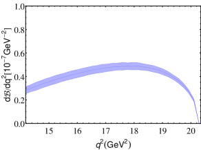
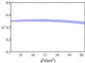
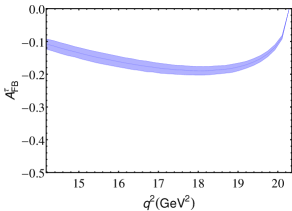
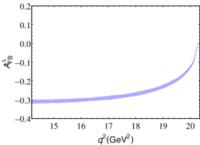
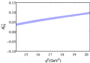
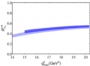
Figure 1: The SM predictions of various $\Lambda_{b}\to\Lambda(\to p^{+}\pi^{-})\tau^{+}\tau^{-}$ observables as a function of $q^{2}$. The $R^{\tau/e}_{\Lambda}$ is shown as a function of the upper limit of integration $q^{2}_{\rm max}$ for two values of lower integration limit $q^{2}_{\rm min}=14$ GeV² (light blue) and $q^{2}_{\rm min}=15$ GeV² (dark blue). The bands correspond to the uncertainties discussed in text. Since the OPE at large $q^{2}$ does not capture local resonance structures, the distributions can be locally off from the OPE predictions.

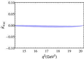
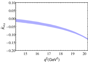
Figure 2: The SM predictions of $\hat{K}_{4sc}$ and $\hat{K}_{4s}$ for $\Lambda_{b}\to\Lambda(\to p^{+}\pi^{-})\tau^{+}\tau^{-}$ as a function of $q^{2}$. The bands correspond to the uncertainties discussed in text. Since the OPE at large $q^{2}$ does not capture local resonance structures, the distributions can be locally off from the OPE predictions.

For the SM analysis we set the couplings ${\mathcal{C}}_{V,A}^{(\prime)}=0,{\mathcal{C}}_{S,P}^{(\prime)}=0$. The SM Wilson coefficient ${\mathcal{C}}_{7,9}^{\rm eff}$ (see Appendix A) whose dominant contributions come from the short-distance corrections to $\mathcal{O}_{7,9}$, also contain the leading contributions from the factorizable non-local matrix elements of the purely hadronic operators $\mathcal{O}_{1-6,8}$ with quark electro-magnetic current Grinstein:2004vb ; Beylich:2011aq . The sub-leading contributions from an operator product expansion (OPE) Beylich:2011aq arise from dimension-5 operators, whose matrix elements are suppressed at high-$q^{2}$ by $\Lambda_{\rm had}^{2}/Q^{2}\sim 2\%$, where $Q^{2}\sim\{q^{2},m_{b}^{2}\}$. We ignore the yet to be derived non-factorizable spectator corrections for baryonic decay which are expected to be significant only at the low-$q^{2}$ region. However, the perturbative expressions of ${\mathcal{C}}_{7,9}^{\rm eff}$ given in Appendix A do not accurately describe the effects of multiple broad charmonium resonances at high-$q^{2}$ Lyon:2014hpa , which lead to the violation of quark-hadron duality. In the OPE based approach, these are beyond the neglected orders in $\alpha_{s}$ and $\Lambda_{\rm had}/Q$. The duality violation in $B\to K\ell^{+}\ell^{-}$ was estimated to be around 2% for the decay rate integrated over the high-$q^{2}$ region Beylich:2011aq . Since a detailed discussion of quark-hadron duality violation in $\Lambda_{b}\to\Lambda(\to p\pi)\tau^{+}\tau^{-}$ is beyond the scope of this paper, following Detmold:2016pkz we include 5% corrections to both ${\mathcal{C}}_{7,9}^{\rm eff}$ in our analysis to account for this effect. In addition to this correction, the $q^{2}$ distributions of observables, that we discuss next, come with a caveat; since the non-perturbative effects of local resonance structures are not captured by the OPE at any order in perturbation expansion, the distributions can be locally away from the OPE predictions by large amount. Even for observables integrated over the entire low recoil region, the effects can still be significant.

The central values and uncertainties of some of the inputs including the value of the parity violating parameter $\alpha_{\Lambda}$ are collected in table LABEL:tab:inputs in Appendix E while the rest are discussed in the text. The $q^{2}$ distributions of the SM differential branching ratio, the longitudinal polarization fraction $F_{L}$, and three angular asymmetries $A_{\rm FB}^{\tau,\Lambda,\tau\Lambda}$ are shown in figure 1. To obtain the plots the lattice QCD form factors are employed as discussed in Sec. 6. The bands correspond to the uncertainties of the form factors and other inputs. From the plot of the differential branching ratio $d\mathcal{B}/dq^{2}$ we see that the branching ratio is reduced compared to $\Lambda_{b}\to\Lambda\mu^{+}\mu^{-}$ by phase space suppression factor $\beta_{\ell}$. For the angular asymmetries $A^{\tau}_{\rm FB}$ ($A^{\tau\Lambda}_{\rm FB}$) the mass corrections terms to $K_{1c}$ ($K_{2c}$), i.e., $\mathcal{K}_{1c}^{\prime,\prime\prime}$ ($\mathcal{K}_{2c}^{\prime,\prime\prime}$) vanish in the SM. Therefore the effect of lepton mass mainly come due to normalization by the differential decay width and the factor $\beta_{\ell}$ appearing in $\mathcal{K}_{1c}$ ($\mathcal{K}_{2c}$). In the last panel of Fig. 1 we have shown $R^{\tau/e}_{\Lambda_{b}}$ as a function of $q^{2}_{\rm max}$ for two values of $q^{2}_{\rm min}$. In figure 2 we show the angular coefficients $\hat{K}_{4sc}$ and $\hat{K}_{4s}$. For the observable $\hat{K}_{4s}$, in the numerator the mass correction term $\mathcal{K}_{4s}^{\prime\prime}=0$ and $\mathcal{K}_{4s}^{\prime}=0$ in the SM. The effect of lepton mass therefore comes due to the normalization by the branching ratio and through the factor $\beta_{\ell}$ that appear in $\mathcal{K}_{4s}$.

$[q^{2}_{\rm min},q^{2}_{\rm max}]$	$\langle\mathcal{B}\rangle\times 10^{7}$	$\langle F_{L}\rangle$	$\langle A_{\rm FB}^{\tau}\rangle$	$\langle A_{\rm FB}^{\Lambda}\rangle$
[14,15]	$0.31\pm 0.03$	$0.350\pm 0.007$	$-0.120\pm 0.016$	$-0.309\pm 0.009$
[15,16]	$0.39\pm 0.03$	$0.354\pm 0.009$	$-0.149\pm 0.017$	$-0.304\pm 0.009$
[16,18]	$0.93\pm 0.06$	$0.353\pm 0.010$	$-0.180\pm 0.015$	$-0.289\pm 0.009$
[18,20]	$0.83\pm 0.05$	$0.346\pm 0.010$	$-0.173\pm 0.010$	$-0.227\pm 0.009$
[15,20]	$2.16\pm 0.13$	$0.351\pm 0.009$	$-0.171\pm 0.014$	$-0.268\pm 0.008$

Table 1: The total integrated branching ratio and the values of the observables in different $q^{2}$ bins (in GeV²). The errors correspond to the uncertainties discussed in text.

$[q^{2}_{\rm min},q^{2}_{\rm max}]$	$\langle A^{\tau\Lambda}_{\rm FB}\rangle$	$\langle\hat{K}_{4sc}\rangle$	$\langle\hat{K}_{4s}\rangle$
[14,15]	$0.041\pm 0.005$	$-0.0026\pm 0.0030$	$-0.0148\pm 0.0086$
[15,16]	$0.052\pm 0.006$	$-0.0037\pm 0.0036$	$-0.0243\pm 0.0089$
[16,18]	$0.067\pm 0.006$	$-0.0053\pm 0.0035$	$-0.0446\pm 0.0075$
[18,20]	$0.084\pm 0.005$	$-0.0053\pm 0.0028$	$-0.0827\pm 0.0050$
[15,20]	$0.071\pm 0.005$	$-0.0050\pm 0.0031$	$-0.0055\pm 0.0067$

Table 2: The values of the observables in different $q^{2}$ bins (in GeV²). The errors correspond to the uncertainties discussed in text.

In tables 1 and 2 we present the values of the observables in different di-lepton invariant mass squared bins. To be more precise, we have shown the total integrated branching ratio which defined as

$$\langle\mathcal{B}\rangle=\displaystyle\int_{q^{2}_{\rm min}}^{q^{2}_{\rm max}}dq^{2}\frac{d\mathcal{B}}{dq^{2}}\,.$$ (60)

The binned averaged values of an observables such as $\langle F_{L}\rangle$ is defined as

$$\langle F_{L}\rangle=\frac{\displaystyle\int_{q^{2}_{\rm min}}^{q^{2}_{\rm max}}dq^{2}(2K_{1ss}-K_{1cc})}{\displaystyle\int_{q^{2}_{\rm min}}^{q^{2}_{\rm max}}dq^{2}(2K_{2ss}+K_{2cc})}\,.$$ (61)

The $q^{2}$-integrated values of $R^{\tau/e}_{\Lambda_{b}}$ for two different low recoil bins are given below

$$\begin{split}R^{\tau/e}_{\Lambda_{b}}&=&0.5077\pm 0.0210\,,\quad[14-({m_{\Lambda_{b}}}-{m_{\Lambda}})^{2}]~{}\text{GeV}^{2}\,,\\ R^{\tau/e}_{\Lambda_{b}}&=&0.5315\pm 0.0189\,,\quad[15-({m_{\Lambda_{b}}}-{m_{\Lambda}})^{2}]~{}\text{GeV}^{2}\,.\end{split}$$ (62)

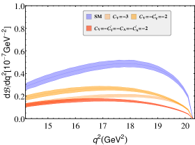
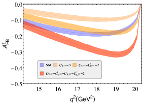
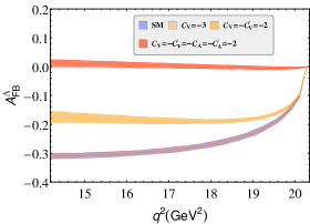
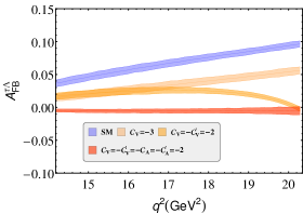
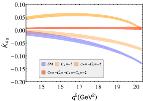
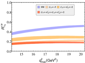
Figure 3: The $\Lambda_{b}\to\Lambda(\to p\pi)\tau^{+}\tau^{-}$ observables in the presence of VA couplings. The bands correspond to the uncertainties discussed in text. Since the OPE at large $q^{2}$ does not capture local resonance structures, the distributions can be locally off from the OPE predictions.

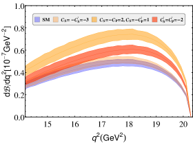
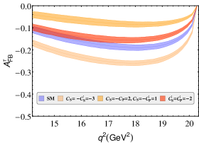
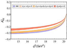
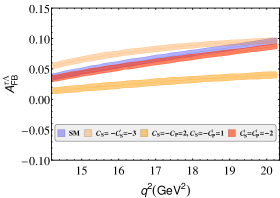
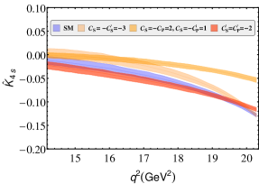
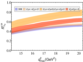
Figure 4: The $\Lambda_{b}\to\Lambda(\to p\pi)\tau^{+}\tau^{-}$ observables in the presence of SP couplings. The bands correspond to the uncertainties discussed in text. Since the OPE at large $q^{2}$ does not capture local resonance structures, the distributions can be locally off from the OPE predictions.

We now discuss the observables in the presence of the NP couplings. The VA and the SP couplings will be considered separately. Due to nonavailability of any data on $b\to s\tau^{+}\tau^{-}$ transition, currently the new physics couplings are very poorly constrained. For VA couplings, following Kamenik:2017ghi we consider the following three scenarios

$${\mathcal{C}}_{V} = -3\,$$

$${\mathcal{C}}_{V} = -{\mathcal{C}}_{V}^{\prime}=-2\,$$ (63)

$${\mathcal{C}}_{V} = -{\mathcal{C}}_{V}^{\prime}=-{\mathcal{C}}_{A}=-{\mathcal{C}}_{A}^{\prime}=-2\,.$$

These ranges of couplings are consistent with the existing direct bounds on $B\to K^{+}\tau^{+}\tau^{-}$ Bobeth:2011st and $B_{s}\to\tau^{+}\tau^{-}$ Aaij:2017xqt , and the bounds on $B\to K^{\ast}\nu\bar{\nu}$ due to heavy NP respecting SM $SU(2)_{L}$ gauge invariance Alonso:2015sja .

In Fig. 3 we present the effects of ${\mathcal{C}}_{V,A}^{(\prime)}$ couplings. The three cases in (7) are separately considered and in each case the rest of the couplings are SM like. We find that the branching ratio gets reduced for all the three scenarios. The leptonic forward-backward asymmetry can be both greater or smaller than the SM value. Note that in the absence of chirality flipped operators, i.e., when ${\mathcal{C}}_{V,A}^{\prime}=0$, the hadronic forward-backward asymmetry is independent of short-distance Wilson coefficients due to the low recoil symmetry of the form factors Boer:2014kda . This is also the reason why in the scenario ${\mathcal{C}}_{V}=-3$, the $A^{\Lambda}_{\rm FB}$ is SM like as can be seen from Fig. 3. In the last scenario of (7), ${\mathcal{C}}_{V}=-{\mathcal{C}}_{V}^{\prime}=-{\mathcal{C}}_{A}=-{\mathcal{C}}_{A}^{\prime}=-2$ the asymmetry $A^{\Lambda}_{\rm FB}$ has opposite sign than SM. For this scenario we notice sign flip in $A^{\tau\Lambda}_{\rm FB}$ and $\hat{K}_{4sc}$ also. For all the three cases, the value of $R^{\tau/e}_{\Lambda_{b}}$ is smaller than the SM value.

For the scalar couplings, indirect bounds from $b\to s\gamma$ and $b\to s\ell^{+}\ell^{-}$, and direct bounds from the limits on $B_{s}\to\tau^{+}\tau^{-}$ branching ratio, the exclusive semi-leptonic mode $B^{+}\to K^{+}\tau^{+}\tau^{-}$ and its inclusive counterpart $B\to X_{s}\tau^{+}\tau^{-}$ were studied in Bobeth:2011st . The obtained bounds are $|{\mathcal{C}}_{S}\mp{\mathcal{C}}_{P}|<0.4\frac{2\pi}{\alpha_{e}}\,$, $|{\mathcal{C}}_{S}^{\prime}\mp{\mathcal{C}}_{P}^{\prime}|<0.4\frac{2\pi}{\alpha_{e}}\,$ which are extremely weak. Therefore, for illustrative purpose we choose three sets of couplings (i) ${\mathcal{C}}_{S}=-{\mathcal{C}}_{S}^{\prime}=-3$, (ii) ${\mathcal{C}}_{S}=-{\mathcal{C}}_{P}=2,{\mathcal{C}}_{S}=-{\mathcal{C}}_{P}^{\prime}=-1$, and (iii) ${\mathcal{C}}_{S}^{\prime}={\mathcal{C}}_{P}^{\prime}=-2$. In Fig. 4 we show the plots for these three sets of couplings. The branching ratio and hence $R^{\tau/e}_{\Lambda}$ are enhanced for these couplings. However, for these set of couplings we did not notice any sign flip for the asymmetries $A^{\Lambda}_{\rm FB}$ and $A^{\tau\Lambda}_{\rm FB}$.

8 Summary

In this paper we have presented a full angular distribution of $\Lambda_{b}\to\Lambda(\to N\pi)\ell^{+}\ell^{-}$ decay for heavy leptons and unpolarized $\Lambda_{b}$ in an operator basis that includes the SM operators, new vector and axial-vector operators, and scalar and pseudo-scalar operators. We have worked in the transversity basis and expressed the angular coefficients in terms of the transversity amplitudes. The $\Lambda_{b}\to\Lambda$ hadronic matrix elements are parametrized in terms of helicity form factors whose $q^{2}$ dependence are known from fit to calculations in lattice QCD. For our numerical analysis we have studied the mode $\Lambda_{b}\to\Lambda(\to p\pi)\tau^{+}\tau^{-}$. We have presented the SM determinations of several observables including the lepton flavor universality sensitive observable $R^{\tau/e}_{\Lambda_{b}}$. We have also explored the effects of the NP couplings on the observables.

Appendix A SM Wilson coefficients

The standard model effective Wilson coefficients ${\mathcal{C}}_{7,9}^{\rm eff}$ are given as Grinstein:2004vb

$${\mathcal{C}}_{9}^{\rm eff} = \mathcal{C}_{9}^{\rm SM}+h(0,q^{2})\bigg{[}\frac{4}{3}{\mathcal{C}}_{1}+{\mathcal{C}}_{2}+\frac{11}{2}{\mathcal{C}}_{3}-\frac{2}{3}{\mathcal{C}}_{4}+52{\mathcal{C}}_{5}-\frac{32}{3}{\mathcal{C}}_{6}\bigg{]}\,$$ (64)

$$- \frac{1}{2}h(m_{b},q^{2})\bigg{[}7{\mathcal{C}}_{3}+\frac{4}{3}{\mathcal{C}}_{4}+76{\mathcal{C}}_{5}+\frac{64}{3}{\mathcal{C}}_{6}\bigg{]}+\frac{4}{3}\bigg{[}{\mathcal{C}}_{3}+\frac{16}{3}{\mathcal{C}}_{5}+\frac{16}{9}{\mathcal{C}}_{6}\bigg{]}\,$$

$$+ 8\frac{m_{c}^{2}}{q^{2}}\bigg{[}\frac{4}{9}{\mathcal{C}}_{1}+\frac{1}{3}{\mathcal{C}}_{2}+2{\mathcal{C}}_{3}+20{\mathcal{C}}_{5}\bigg{]}\,$$

$$+ \frac{\alpha_{s}}{4\pi}\bigg{[}{\mathcal{C}}_{1}(B(q^{2})+4C(q^{2}))-3{\mathcal{C}}_{2}(2B(q^{2})-C(q^{2}))-{\mathcal{C}}_{8}F_{8}^{(9)}(q^{2})\bigg{]}\,,$$

$${\mathcal{C}}_{7}^{\rm eff} = {\mathcal{C}}_{7}^{\rm SM}-\frac{1}{3}\bigg{[}{\mathcal{C}}_{3}+\frac{4}{3}{\mathcal{C}}_{4}+20{\mathcal{C}}_{5}+\frac{80}{3}{\mathcal{C}}_{6}\bigg{]}+\frac{\alpha_{s}}{4\pi}\bigg{[}({\mathcal{C}}_{1}-6{\mathcal{C}}_{2})A(q^{2})-{\mathcal{C}}_{8}F_{8}^{(7)}(q^{2})\bigg{]}\,,$$ (65)

where $\mathcal{C}_{7,9}^{\rm SM}$ are the SM values at the scale of $b$-quark mass Altmannshofer:2008dz , $\mu=m_{b}=4.8$ GeV. Rest of the Wilson coefficients are also taken from Altmannshofer:2008dz . The charm and the $b$-quark loop functions read Buras:1994dj ; Misiak:1992bc

$$h(m_{q},q^{2}) = -\frac{8}{9}\ln\frac{m_{q}}{m_{b}}+\frac{8}{27}+\frac{4}{9}x-\frac{2}{9}(2+x)|1-x|^{1/2}\left\{\begin{array}[]{ll}\ln\left|\frac{\sqrt{1-x}+1}{\sqrt{1-x}-1}\right|-i\pi,&x\equiv\frac{4m_{c}^{2}}{q^{2}}<1,\\ &\\ 2\arctan\frac{1}{\sqrt{x-1}},&x\equiv\frac{4m_{c}^{2}}{q^{2}}>1,\end{array}\right.$$ (69)

$$h(0,q^{2}) = \frac{8}{27}-\frac{4}{9}\ln\frac{q^{2}}{m_{b}^{2}}+\frac{4}{9}i\pi.$$ (70)

The loop functions $A(q^{2}),B(q^{2}),C(q^{2})$ and $F_{8}^{(7,9)}$ are taken from Beneke:2001at ; Seidel:2004jh .

Appendix B Transversity amplitudes

The $\Lambda_{b}\to\Lambda$ hadronic matrix elements for different operators can be parametrized in terms of ten helicity form factors $f^{V}_{t,0,\perp}$, $f^{A}_{t,0,\perp}$, $f^{T}_{0,\perp}$, $f^{T5}_{0,\perp}$ Feldmann:2011xf and spinor matrix elements. For the operators (2), the hadronic matrix elements parametrization in terms of the spinor bilinears are summarized in Appendix D. The spinor bilinears can be found in the Appendix of Das:2018sms . The helicity amplitudes are defined as the projection of the hadronic matrix elements on to the direction of the polarization of the virtual gauge boson that decays to a dilepton pair. For VA operators the detailed derivations of the helicity amplitudes for massless leptons can be found in Das:2018sms . For completeness we write down their expressions

$$H^{L(R),{+\frac{1}{2}+\frac{1}{2}}}_{\rm VA,0} = f^{V}_{0}({m_{\Lambda_{b}}}+{m_{\Lambda}})\sqrt{\frac{s_{-}}{q^{2}}}{\mathcal{C}}^{L,(R)}_{\rm VA,+}-f^{A}_{0}({m_{\Lambda_{b}}}-{m_{\Lambda}})\sqrt{\frac{s_{+}}{q^{2}}}{\mathcal{C}}^{L,(R)}_{\rm VA,-}\,$$ (71)

$$+ \frac{2m_{b}}{q^{2}}\bigg{(}f^{T}_{0}\sqrt{q^{2}s_{-}}-f^{T5}_{0}\sqrt{q^{2}s_{+}}\bigg{)}{\mathcal{C}}_{7}^{\rm eff}\,,$$

$$H^{L(R),{-\frac{1}{2}-\frac{1}{2}}}_{\rm VA,0} = f^{V}_{0}({m_{\Lambda_{b}}}+{m_{\Lambda}})\sqrt{\frac{s_{-}}{q^{2}}}{\mathcal{C}}^{L,(R)}_{\rm VA,+}+f^{A}_{0}({m_{\Lambda_{b}}}-{m_{\Lambda}})\sqrt{\frac{s_{+}}{q^{2}}}{\mathcal{C}}^{L,(R)}_{\rm VA,-}\,$$ (72)

$$+ \frac{2m_{b}}{q^{2}}\bigg{(}f^{T}_{0}\sqrt{q^{2}s_{-}}+f^{T5}_{0}\sqrt{q^{2}s_{+}}\bigg{)}{\mathcal{C}}_{7}^{\rm eff}\,,$$

$$H^{L(R),{-\frac{1}{2}+\frac{1}{2}}}_{\rm VA,+} = -f^{V}_{\perp}\sqrt{2s_{-}}{\mathcal{C}}^{L,(R)}_{\rm VA,+}+f^{A}_{\perp}\sqrt{2s_{+}}{\mathcal{C}}^{L,(R)}_{\rm VA,-}\,$$ (73)

$$- \frac{2m_{b}}{q^{2}}\bigg{(}f^{T}_{\perp}({m_{\Lambda_{b}}}+{m_{\Lambda}})\sqrt{2s_{-}}-f^{T5}_{\perp}({m_{\Lambda_{b}}}-{m_{\Lambda}})\sqrt{2s_{+}}\bigg{)}{\mathcal{C}}_{7}^{\rm eff}\,,~{}~{}~{}$$

$$H^{L(R),{+\frac{1}{2}-\frac{1}{2}}}_{\rm VA,-} = -f^{V}_{\perp}\sqrt{2s_{-}}{\mathcal{C}}^{L,(R)}_{\rm VA,+}-f^{A}_{\perp}\sqrt{2s_{+}}{\mathcal{C}}^{L,(R)}_{\rm VA,-}\,$$ (74)

$$- \frac{2m_{b}}{q^{2}}\bigg{(}f^{T}_{\perp}({m_{\Lambda_{b}}}+{m_{\Lambda}})\sqrt{2s_{-}}+f^{T5}_{\perp}({m_{\Lambda_{b}}}-{m_{\Lambda}})\sqrt{2s_{+}}\bigg{)}{\mathcal{C}}_{7}^{\rm eff}\,.$$

If the leptons are massive, then there are additional timelike helicity amplitudes that can be defined. The timelike polarization of the gauge boson $\bar{\epsilon}^{\mu}=q^{\mu}/\sqrt{q^{2}}$ leads to the following conservation laws

$$q^{\mu}(\bar{\ell}\gamma_{\mu}\ell)=0\,,\quad q^{\mu}(\bar{\ell}\gamma_{\mu}\gamma_{5}\ell)=2mi(\bar{\ell}\gamma_{5}\ell)\,.$$ (75)

These equations imply that the timelike components of the gauge boson can only couple to the axial-vector current and therefore can not have separate left- and right-handed parts. The two non-vanishing helicity amplitudes that we find are

$$H^{{+\frac{1}{2}+\frac{1}{2}}}_{t} = 2\bigg{(}f^{A}_{t}({m_{\Lambda_{b}}}+{m_{\Lambda}})\sqrt{\frac{s_{-}}{q^{2}}}({\mathcal{C}}_{10}+{\mathcal{C}}_{A}-{\mathcal{C}}_{A}^{\prime})\,$$ (76)

$$- f^{V}_{t}({m_{\Lambda_{b}}}-{m_{\Lambda}})\sqrt{\frac{s_{+}}{q^{2}}}({\mathcal{C}}_{10}+{\mathcal{C}}_{A}+{\mathcal{C}}_{A}^{\prime})\bigg{)}\,,$$

$$H^{{-\frac{1}{2}-\frac{1}{2}}}_{t} = -2\bigg{(}f^{A}_{t}({m_{\Lambda_{b}}}+{m_{\Lambda}})\sqrt{\frac{s_{-}}{q^{2}}}({\mathcal{C}}_{10}+{\mathcal{C}}_{A}-{\mathcal{C}}_{A}^{\prime})\,$$ (77)

$$+ f^{V}_{t}({m_{\Lambda_{b}}}-{m_{\Lambda}})\sqrt{\frac{s_{+}}{q^{2}}}({\mathcal{C}}_{10}+{\mathcal{C}}_{A}+{\mathcal{C}}_{A}^{\prime})\bigg{)}\,.$$

From these helicity amplitudes, we construct the following transversity amplitudes corresponding to the VA currents

$$A_{\perp_{0}}^{L(R)}=\frac{N}{\sqrt{2}}\bigg{[}H^{L(R),{+\frac{1}{2}+\frac{1}{2}}}_{0}+H^{L(R),{-\frac{1}{2}-\frac{1}{2}}}_{0}\bigg{]}\,,$$ (78)

$$A_{\|_{0}}^{L(R)}=\frac{N}{\sqrt{2}}\bigg{[}H^{L(R),{+\frac{1}{2}+\frac{1}{2}}}_{0}-H^{L(R),{-\frac{1}{2}-\frac{1}{2}}}_{0}\bigg{]}\,,$$ (79)

$$A_{\perp_{1}}^{L(R)}=\frac{N}{\sqrt{2}}\bigg{[}H^{L(R),{-\frac{1}{2}+\frac{1}{2}}}_{+}+H^{L(R),{+\frac{1}{2}-\frac{1}{2}}}_{-}\bigg{]}\,,$$ (80)

$$A_{\|_{1}}^{L(R)}=\frac{N}{\sqrt{2}}\bigg{[}H^{L(R),{-\frac{1}{2}+\frac{1}{2}}}_{+}-H^{L(R),{+\frac{1}{2}-\frac{1}{2}}}_{-}\bigg{]}\,,$$ (81)

$$A_{\perp_{t}}=\frac{N}{\sqrt{2}}\bigg{[}H^{{+\frac{1}{2}+\frac{1}{2}}}_{t}+H^{{-\frac{1}{2}-\frac{1}{2}}}_{t}\bigg{]}\,,$$ (82)

$$A_{\|_{t}}=\frac{N}{\sqrt{2}}\bigg{[}H^{{+\frac{1}{2}+\frac{1}{2}}}_{t}-H^{{-\frac{1}{2}-\frac{1}{2}}}_{t}\bigg{]}\,,$$ (83)

The helicty amplitudes corresponding to the scalar operators are derived in details in Ref. Das:2018sms . Here we define the transversity amplitudes in terms of them

$$A_{\rm S\perp}=\frac{N}{\sqrt{2}}\bigg{[}H^{L,{+\frac{1}{2}+\frac{1}{2}}}_{\rm SP}+H^{R,{+\frac{1}{2}+\frac{1}{2}}}_{\rm SP}+H^{L,{-\frac{1}{2}-\frac{1}{2}}}_{\rm SP}+H^{R,{-\frac{1}{2}-\frac{1}{2}}}_{\rm SP}\bigg{]}\,,$$ (84)

$$A_{\rm S\|}=\frac{N}{\sqrt{2}}\bigg{[}H^{L,{+\frac{1}{2}+\frac{1}{2}}}_{\rm SP}+H^{R,{+\frac{1}{2}+\frac{1}{2}}}_{\rm SP}-H^{L,{-\frac{1}{2}-\frac{1}{2}}}_{\rm SP}-H^{R,{-\frac{1}{2}-\frac{1}{2}}}_{\rm SP}\bigg{]}\,,$$ (85)

$$A_{\rm P\perp}=\frac{N}{\sqrt{2}}\bigg{[}H^{L,{+\frac{1}{2}+\frac{1}{2}}}_{\rm SP}-H^{R,{+\frac{1}{2}+\frac{1}{2}}}_{\rm SP}+H^{L,{-\frac{1}{2}-\frac{1}{2}}}_{\rm SP}-H^{R,{-\frac{1}{2}-\frac{1}{2}}}_{\rm SP}\bigg{]}\,,$$ (86)

$$A_{\rm P\|}=\frac{N}{\sqrt{2}}\bigg{[}H^{L,{+\frac{1}{2}+\frac{1}{2}}}_{\rm SP}-H^{R,{+\frac{1}{2}+\frac{1}{2}}}_{\rm SP}-H^{L,{-\frac{1}{2}-\frac{1}{2}}}_{\rm SP}+H^{R,{-\frac{1}{2}-\frac{1}{2}}}_{\rm SP}\bigg{]}\,.$$ (87)

Appendix C Angular coefficients

From Sec. 5 we recall that the angular coefficients are written as

$$K_{\{\cdots\}}=\mathcal{K}_{\{\cdots\}}+\frac{m_{\ell}}{\sqrt{q^{2}}}\mathcal{K}_{\{\cdots\}}^{\prime}+\frac{m_{\ell}^{2}}{q^{2}}\mathcal{K}_{\{\cdots\}}^{\prime\prime}\,,$$ (88)

where $\{\cdots\}$ correspond to the suffixes $1ss,1cc,1c,2ss,2cc,2c,3sc,3s,4sc,4s$. In terms of the transversity amplitudes the expressions of $\mathcal{K},\mathcal{K}^{\prime}\mathcal{K}^{\prime\prime}$ read as

$${\mathcal{K}}_{1ss} = \frac{1}{4}\bigg{(}2|{A^{R}_{\|_{0}}}|^{2}+|{A^{R}_{\|_{1}}}|^{2}+2|{A^{R}_{\perp_{0}}}|^{2}+|{A^{R}_{\perp_{1}}}|^{2}+\{R\leftrightarrow L\}\bigg{)}$$ (89)

$$+ \frac{1}{4}\bigg{(}|A_{\rm S\perp}|^{2}+|A_{\rm P\perp}|^{2}+\{\perp\leftrightarrow\|\}\bigg{)}\,,~{}~{}~{}~{}$$

$${\mathcal{K}}_{1ss}^{\prime} = {\rm Re}\bigg{(}A_{\|t}A_{\rm P\|}^{\ast}+A_{\perp t}A^{\ast}_{\rm P\perp}\bigg{)}\,,$$ (90)

$${\mathcal{K}}_{1ss}^{\prime\prime} = -\bigg{(}|A^{R}_{\|_{0}}|^{2}+|A^{R}_{\perp_{0}}|^{2}+\{R\leftrightarrow L\}\bigg{)}+\bigg{(}|A_{\perp t}|^{2}-|A_{\rm S\perp}|+\{\perp\leftrightarrow\|\}\bigg{)}$$ (91)

$$+ 2{\rm Re}\bigg{(}A^{R}_{\perp_{0}}A^{\ast L}_{\perp_{0}}+A^{R}_{\perp_{1}}A^{\ast L}_{\perp_{1}}+\{\perp\leftrightarrow\|\}\bigg{)}\,,$$

$${\mathcal{K}}_{1cc} = \frac{1}{2}\bigg{(}|{A^{R}_{\|_{1}}}|^{2}+|{A^{R}_{\perp_{1}}}|^{2}+\{R\leftrightarrow L\}\bigg{)}+\frac{1}{4}\bigg{(}|A_{\rm P\perp}|^{2}+|A_{\rm S\perp}|^{2}+\{\perp\leftrightarrow\|\}\bigg{)}\,,$$ (92)

$${\mathcal{K}}_{1cc}^{\prime} = {\rm Re}\bigg{(}A_{\|t}A^{\ast}_{\rm P\|}+A_{\perp t}A^{\ast}_{\rm P\perp}\bigg{)},$$ (93)

$${\mathcal{K}}_{1cc}^{\prime\prime} = \bigg{(}|A^{R}_{\|_{0}}|^{2}-|A^{R}_{\|_{1}}|^{2}+|A^{R}_{\perp_{0}}|^{2}-|A^{R}_{\perp_{1}}|^{2}+\{R\leftrightarrow L\}\bigg{)}+\bigg{(}|A_{\perp t}|^{2}-|A_{\rm S\perp}|^{2}+\{\perp\leftrightarrow\|\}\bigg{)}\,$$ (94)

$$+ 2{\rm Re}\bigg{(}A^{R}_{\perp_{0}}A^{\ast L}_{\perp_{0}}+A^{R}_{\perp_{1}}A^{\ast L}_{\perp_{1}}+\{\perp\leftrightarrow\|\}\bigg{)}\,,$$

$${\mathcal{K}}_{1c} = -\beta_{\ell}\bigg{(}A^{R}_{\perp_{1}}A^{\ast R}_{\|_{1}}-\{R\leftrightarrow L\}\bigg{)}\,,$$ (95)

$${\mathcal{K}}_{1c}^{\prime} = \beta_{\ell}{\rm Re}\bigg{(}A_{\rm S\perp}A^{\ast R}_{\perp_{0}}+A_{\rm S\perp}A^{\ast L}_{\perp_{0}}+\{\perp\leftrightarrow\|\}\bigg{)}\,,$$ (96)

$${\mathcal{K}}_{1c}^{\prime\prime} = 0\,,$$ (97)

$${\mathcal{K}}_{2ss} = \frac{\alpha_{\Lambda}}{2}{\rm Re}\bigg{(}2A^{R}_{\perp_{0}}A^{\ast R}_{\|_{0}}+A^{R}_{\perp_{1}}A^{\ast R}_{\|_{1}}+\{R\leftrightarrow L\}\bigg{)}+\frac{\alpha_{\Lambda}}{2}{\rm Re}\bigg{(}A_{\rm P\perp}A^{\ast}_{\rm P\|}+A_{\rm S\perp}A^{\ast}_{\rm S\|}\bigg{)}\,,$$ (98)

$${\mathcal{K}}_{2ss}^{\prime} = \alpha_{\Lambda}{\rm Re}\bigg{(}A_{\perp t}A^{\ast}_{\rm P\|}+A_{\|t}A^{\ast}_{\rm P\perp}\bigg{)}\,,$$ (99)

$${\mathcal{K}}_{2ss}^{\prime\prime} = -2\alpha_{\Lambda}{\rm Re}\bigg{(}A^{R}_{\perp_{0}}A^{\ast R}_{\|_{0}}+A^{L}_{\perp_{0}}A^{\ast L}_{\|_{0}}-A^{R}_{\perp_{0}}A^{\ast L}_{\|_{0}}-A^{R}_{\|_{0}}A^{\ast L}_{\perp_{0}}-A^{R}_{\perp_{1}}A^{\ast L}_{\|_{1}}-A^{R}_{\|_{1}}A^{\ast L}_{\perp_{1}}$$ (100)

$$- A_{\perp t}A^{\ast}_{\|t}+A_{\rm S\perp}A^{\ast}_{\rm S\|}\bigg{)}\,,$$

$${\mathcal{K}}_{2cc} = \alpha_{\Lambda}{\rm Re}\bigg{(}A^{R}_{\perp_{1}}A^{\ast R}_{\|_{1}}+A^{L}_{\perp_{1}}A^{\ast L}_{\|_{1}}\bigg{)}+\frac{\alpha_{\Lambda}}{2}{\rm Re}\bigg{(}A_{\rm P\perp}A^{\ast}_{\rm P\|}+A_{\rm S\perp}A^{\ast}_{\rm S\|}\bigg{)}\,,$$ (101)

$${\mathcal{K}}_{2cc}^{\prime} = \alpha_{\Lambda}{\rm Re}\bigg{(}A_{\perp t}A^{\ast}_{\rm P\|}+A_{\|t}A^{\ast}_{\rm P\perp}\bigg{)}\,,$$ (102)

$${\mathcal{K}}_{2cc}^{\prime\prime} = -2\alpha_{\Lambda}{\rm Re}\bigg{(}A^{R}_{\perp_{1}}A^{\ast R}_{\|_{1}}-A^{R}_{\perp_{0}}A^{\ast R}_{\|_{0}}+A^{L}_{\perp_{1}}A^{\ast L}_{\|_{1}}-A^{L}_{\perp_{0}}A^{\ast L}_{\|_{0}}-A^{R}_{\perp_{0}}A^{\ast L}_{\|_{0}}-A^{R}_{\|_{0}}A^{\ast L}_{\perp_{0}}$$ (103)

$$- A^{R}_{\perp_{1}}A^{\ast L}_{\|_{1}}-A^{R}_{\|_{1}}A^{\ast L}_{\perp_{1}}-A_{\perp t}A^{\ast}_{\|t}+A_{\rm S\perp}A^{\ast}_{\rm S\|}\bigg{)}\,,$$

$${\mathcal{K}}_{2c} = -\frac{\alpha_{\Lambda}\beta_{\ell}}{2}{\rm Re}\bigg{(}|{A^{R}_{\perp_{1}}}|^{2}+|{A^{R}_{\|_{1}}}|^{2}-\{R\leftrightarrow L\}\bigg{)}\,,$$ (104)

$${\mathcal{K}}_{2c}^{\prime} = \alpha_{\Lambda}\beta_{\ell}{\rm Re}\bigg{(}A_{\rm S\perp}A^{\ast R}_{\|_{0}}+A_{\rm S\|}A^{\ast R}_{\perp_{0}}+\{R\leftrightarrow L\}\bigg{)}\,,$$ (105)

$${\mathcal{K}}_{2c}^{\prime\prime} = 0\,,$$ (106)

$${\mathcal{K}}_{3sc} = \frac{\alpha_{\Lambda}}{\sqrt{2}}{\rm Im}\bigg{(}{A^{R}_{\perp_{1}}}{A^{\ast R}_{\perp_{0}}}-{A^{R}_{\|_{1}}}{A^{\ast R}_{\|_{0}}}+\{R\leftrightarrow L\}\bigg{)}\,,$$ (107)

$${\mathcal{K}}_{3sc}^{\prime} = 0\,,$$ (108)

$${\mathcal{K}}_{3sc}^{\prime\prime} = 2\sqrt{2}\alpha_{\Lambda}{\rm Im}\bigg{(}A^{R}_{\|_{1}}A^{\ast R}_{\|_{0}}-A^{R}_{\perp_{1}}A^{\ast R}_{\perp_{0}}+\{R\leftrightarrow L\}\bigg{)}\,,$$ (109)

$${\mathcal{K}}_{3s} = \frac{\alpha_{\Lambda}\beta_{\ell}}{\sqrt{2}}{\rm Im}\bigg{(}A^{R}_{\perp_{1}}A^{\ast R}_{\|_{0}}-A^{R}_{\|_{1}}A^{\ast R}_{\perp_{0}}-\{R\leftrightarrow L\}\bigg{)}\,,$$ (110)

$${\mathcal{K}}_{3s}^{\prime} = \frac{\alpha_{\Lambda}\beta_{\ell}}{\sqrt{2}}{\rm Im}\bigg{(}A^{R}_{\|_{1}}A^{\ast}_{\rm S\|}-A^{R}_{\perp_{1}}A^{\ast}_{\rm S\perp}+\{R\leftrightarrow L\}\bigg{)}\,,$$ (111)

$${\mathcal{K}}_{3s}^{\prime\prime} = 0\,,$$ (112)

$${\mathcal{K}}_{4sc} = \frac{\alpha_{\Lambda}}{\sqrt{2}}{\rm Re}\bigg{(}A^{R}_{\perp_{1}}A^{\ast R}_{\|_{0}}-A^{R}_{\|_{1}}A^{\ast R}_{\perp_{0}}+\{R\leftrightarrow L\}\bigg{)}\,,$$ (113)

$${\mathcal{K}}_{4sc}^{\prime} = 0\,,$$ (114)

$${\mathcal{K}}_{4sc}^{\prime\prime} = 2\sqrt{2}\alpha_{\Lambda}{\rm Re}\bigg{(}A^{R}_{\|_{1}}A^{\ast R}_{\perp_{0}}-A^{R}_{\perp_{1}}A^{\ast R}_{\|_{0}}+\{R\leftrightarrow L\}\bigg{)}\,,$$ (115)

$${\mathcal{K}}_{4s} = \frac{\alpha_{\Lambda}\beta_{\ell}}{\sqrt{2}}{\rm Re}\bigg{(}A^{R}_{\perp_{1}}A^{\ast R}_{\perp_{0}}-A^{R}_{\|_{1}}A^{\ast R}_{\|_{0}}-\{R\leftrightarrow L\}\bigg{)}\,,$$ (116)

$${\mathcal{K}}_{4s}^{\prime} = \frac{\alpha_{\Lambda}\beta_{\ell}}{\sqrt{2}}{\rm Re}\bigg{(}A^{R}_{\|_{1}}A^{\ast}_{\rm S\perp}-A^{R}_{\perp_{1}}A^{\ast}_{\rm S\|}+A_{\rm S\perp}A^{\ast R}_{\|_{1}}-A_{\rm S\|}A^{\ast R}_{\perp_{1}}+\{R\leftrightarrow L\bigg{)}\,,$$ (117)

$${\mathcal{K}}_{4s}^{\prime\prime} = 0\,.$$ (118)

For our SM results, we agree with Blake:2017une

Appendix D $\Lambda_{b}\to\Lambda$ hadronic matrix elements

A convenient choice for the parametrization of the $\Lambda_{b}\to\Lambda$ hadronic matrix elements is the so called helicty basis Feldmann:2011xf in terms of which the matrix elements for the vector current is

$$\langle\Lambda(k,s_{k})|\bar{s}\gamma^{\mu}b|\Lambda(p,s_{p})\rangle= \bar{u}(k,s_{k})\Bigg{[}f^{V}_{t}(q^{2})({m_{\Lambda_{b}}}-{m_{\Lambda}})\frac{q^{\mu}}{q^{2}}$$

$$+ f^{V}_{0}(q^{2})\frac{{m_{\Lambda_{b}}}+{m_{\Lambda}}}{s_{+}}\{p^{\mu}+k^{\mu}-\frac{q^{\mu}}{q^{2}}({m^{2}_{\Lambda_{b}}}-{m^{2}_{\Lambda}})\}$$

$$+ f^{V}_{\perp}(q^{2})\{\gamma^{\mu}-\frac{2{m_{\Lambda}}}{s_{+}}p^{\mu}-\frac{2{m_{\Lambda_{b}}}}{s_{+}}k^{\mu}\}\Bigg{]}u(p,s_{p})\,,$$ (119)

and the axial-vector current is

$$\langle\Lambda(k,s_{k})|\bar{s}\gamma^{\mu}\gamma_{5}b|\Lambda(p,s_{p})\rangle= -\bar{u}(k,s_{k})\gamma_{5}\Bigg{[}f_{t}^{A}(q^{2})({m_{\Lambda_{b}}}+{m_{\Lambda}})\frac{q^{\mu}}{q^{2}}$$

$$+ f_{0}^{A}(q^{2})\frac{{m_{\Lambda_{b}}}-{m_{\Lambda}}}{s_{-}}\{p^{\mu}+k^{\mu}-\frac{q^{\mu}}{q^{2}}({m^{2}_{\Lambda_{b}}}-{m^{2}_{\Lambda}})\}$$

$$+ f_{\perp}^{A}(q^{2})\{\gamma^{\mu}+\frac{2{m_{\Lambda}}}{s_{-}}p^{\mu}-\frac{2{m_{\Lambda_{b}}}}{s_{-}}k^{\mu}\}\Bigg{]}u(p,s_{p})\,.$$ (120)

The matrix elements for the scalar and the pseudo-scalar currents are

$$\langle\Lambda(k,s_{k})|\bar{s}b|\Lambda(p,s_{p})\rangle= f^{V}_{t}(q^{2})\frac{{m_{\Lambda_{b}}}-{m_{\Lambda}}}{m_{b}}\bar{u}(k,s_{k})u(p,s_{p})\,,$$ (121)

$$\langle\Lambda(k,s_{k})|\bar{s}\gamma_{5}b|\Lambda(p,s_{p})\rangle= f_{t}^{A}(q^{2})\frac{{m_{\Lambda_{b}}}+{m_{\Lambda}}}{m_{b}}\bar{u}(k,s_{k})\gamma_{5}u(p,s_{p})\,,$$ (122)

where we have neglected the mass of the strange quark. For the dipole operators we get

$$\langle\Lambda|\bar{s}iq_{\nu}\sigma^{\mu\nu}b|\Lambda_{b}\rangle = -\bar{u}(k,s_{k})\Bigg{[}f^{T}_{0}(q^{2})\frac{q^{2}}{s_{+}}\Bigg{(}p^{\mu}+k^{\mu}-\frac{q^{\mu}}{q^{2}}({m^{2}_{\Lambda_{b}}}-{m^{2}_{\Lambda}})\Bigg{)}\,$$ (123)

$$+ f^{T}_{\perp}({m_{\Lambda_{b}}}+{m_{\Lambda}})\Bigg{(}\gamma^{\mu}-\frac{2{m_{\Lambda}}}{s_{+}}p^{\mu}-\frac{2{m_{\Lambda_{b}}}}{s_{+}}k^{\mu}\Bigg{)}\Bigg{]}u(p,s_{p})\,,$$

and

$$\langle\Lambda|\bar{s}iq_{\nu}\sigma^{\mu\nu}\gamma_{5}b|\Lambda_{b}\rangle = -\bar{u}(k,s_{k})\gamma_{5}\Bigg{[}f^{T5}_{0}\frac{q^{2}}{s_{-}}\Bigg{(}p^{\mu}+k^{\mu}-\frac{q^{\mu}}{q^{2}}({m^{2}_{\Lambda_{b}}}-{m^{2}_{\Lambda}})\Bigg{)}\,$$ (124)

$$+ f^{T5}_{\perp}({m_{\Lambda_{b}}}-{m_{\Lambda}})\Bigg{(}\gamma^{\mu}+\frac{2{m_{\Lambda}}}{s_{-}}p^{\mu}-\frac{2{m_{\Lambda_{b}}}}{s_{-}}k^{\mu}\Bigg{)}\Bigg{]}u(p,s_{p})\,.$$

Appendix E Numerical inputs

In the following table we collect the numerical values of the inputs used in the paper.

Table 3: List of inputs and their values.

inputs	values	inputs	values
$\alpha_{e}(m_{b})$	$1/127.925(16)$ Patrignani:2016xqp	$|V_{tb}V_{ts}^{\ast}|$	$0.0401\pm 0.0010$ Bona:2006ah
$m_{c}(\overline{\text{MS}})$	1.28 GeV Patrignani:2016xqp	${m_{\Lambda_{b}}}$	5.619 GeV Patrignani:2016xqp
$\mu_{b}$	$4.8$ GeV Altmannshofer:2008dz	${m_{\Lambda}}$	$1.115$ GeV Patrignani:2016xqp
$m_{b}(\overline{\text{MS}})$	$4.2$ GeV Altmannshofer:2008dz	$\tau_{\Lambda_{b}}$	$(1.470\pm 0.010)\times 10^{-12}s$ Patrignani:2016xqp
$m_{b}({\rm pole})$	$4.8$ GeV Altmannshofer:2008dz	$m_{B^{0}}$	$5.279$ GeV Detmold:2016pkz
$\alpha_{s}(m_{b})$	$0.214$ Altmannshofer:2008dz	$m_{K}$	$0.494$ GeV Detmold:2016pkz
$|V_{cb}|$	$(4.15\pm 0.07)\times 10^{-2}$ Bona:2006ah	$\alpha_{\Lambda}$	$0.642\pm 0.013$ Patrignani:2016xqp
$\alpha_{s}(M_{Z})$	$0.1181\pm 0.0011$ Patrignani:2016xqp	$m_{c}(m_{c})$	$1.28\pm 0.03$ GeV Patrignani:2016xqp

References

• (1) F.Β Kruger, L.Β M.Β Sehgal, N.Β Sinha and R.Β Sinha, Angular distribution and CP asymmetries in the decays $\bar{B}\to K^{-}\pi^{+}e^{-}e^{+}$ and $\bar{B}\to\pi^{-}\pi^{+}e^{-}e^{+}$, Phys.Β Rev.Β D 61, 114028 (2000), Erratum: [Phys.Β Rev.Β D 63, 019901 (2001)], [hep-ph/9907386].
• (2) R.Β Aaij et al. [LHCb Collaboration], Differential branching fraction and angular analysis of $\Lambda^{0}_{b}\rightarrow\Lambda\mu^{+}\mu^{-}$ decays, JHEP 1506, 115 (2015), [arXiv:1503.07138 [hep-ex]].
• (3) T.Β Aaltonen et al. [CDF Collaboration], Observation of the Baryonic Flavor-Changing Neutral Current Decay $\Lambda_{b}\to\Lambda\mu^{+}\mu^{-}$ Phys.Β Rev.Β Lett.Β  107, 201802 (2011), [arXiv:1107.3753 [hep-ex]].
• (4) P.Β BΓΆer, T.Β Feldmann and D.Β van Dyk, Angular Analysis of the Decay $\Lambda_{b}\to\Lambda(\to N\pi)\ell^{+}\ell^{-}$, JHEP 1501, 155 (2015), [arXiv:1410.2115 [hep-ph]].
• (5) T.Β Blake and M.Β Kreps, Angular distribution of polarised $\Lambda_{b}$ baryons decaying to $\Lambda\ell^{+}\ell^{-}$, JHEP 1711, 138 (2017), [arXiv:1710.00746 [hep-ph]].
• (6) C.Β Bobeth, M.Β Misiak and J.Β Urban, Photonic penguins at two loops and $m_{t}$ dependence of $BR[B\to X_{s}l^{+}l^{-}]$, Nucl.Β Phys.Β B 574, 291 (2000), [hep-ph/9910220].
• (7) T.Β Feldmann and M.Β W.Β Y.Β Yip, Form Factors for $\Lambda_{b}\to\Lambda$ Transitions in SCET, Phys.Β Rev.Β D 85, 014035 (2012), Erratum: [Phys.Β Rev.Β D 86, 079901 (2012)], [arXiv:1111.1844 [hep-ph]].
• (8) A.Β Ali, C.Β Hambrock, A.Β Y.Β Parkhomenko and W.Β Wang, Light-Cone Distribution Amplitudes of the Ground State Bottom Baryons in HQET, Eur.Β Phys.Β J.Β C 73, no. 2, 2302 (2013), [arXiv:1212.3280 [hep-ph]].
• (9) G.Β Bell, T.Β Feldmann, Y.Β M.Β Wang and M.Β W.Β Y.Β Yip, Light-Cone Distribution Amplitudes for Heavy-Quark Hadrons, JHEP 1311, 191 (2013), [arXiv:1308.6114 [hep-ph]].
• (10) V.Β M.Β Braun, S.Β E.Β Derkachov and A.Β N.Β Manashov, Integrability of the evolution equations for heavy–light baryon distribution amplitudes, Phys.Β Lett.Β B 738, 334 (2014), [arXiv:1406.0664 [hep-ph]].
• (11) Y.Β m.Β Wang, Y.Β Li and C.Β D.Β Lu, Rare Decays of $\Lambda_{b}\to\Lambda+\gamma$ and $\Lambda_{b}\to\Lambda+\ell^{+}\ell^{-}$ in the light-cone sum rules, Eur.Β Phys.Β J.Β C 59, 861 (2009), [arXiv:0804.0648 [hep-ph]].
• (12) Y.Β M.Β Wang and Y.Β L.Β Shen, Perturbative Corrections to $\Lambda_{b}\to\Lambda$ Form Factors from QCD Light-Cone Sum Rules, JHEP 1602, 179 (2016), [arXiv:1511.09036 [hep-ph]].
• (13) W.Β Wang, Factorization of Heavy-to-Light Baryonic Transitions in SCET, Phys.Β Lett.Β B 708, 119 (2012), [arXiv:1112.0237 [hep-ph]].
• (14) T.Β Mannel and Y.Β M.Β Wang, Heavy-to-light baryonic form factors at large recoil, JHEP 1112, 067 (2011), [arXiv:1111.1849 [hep-ph]].
• (15) R.Β N.Β Faustov and V.Β O.Β Galkin, Rare $\Lambda_{b}\to\Lambda l^{+}l^{-}$ and $\Lambda_{b}\to\Lambda\gamma$ decays in the relativistic quark model, Phys.Β Rev.Β D 96, no. 5, 053006 (2017), [arXiv:1705.07741 [hep-ph]].
• (16) W.Β Detmold and S.Β Meinel, $\Lambda_{b}\to\Lambda\ell^{+}\ell^{-}$ form factors, differential branching fraction, and angular observables from lattice QCD with relativistic $b$ quarks, Phys.Β Rev.Β D 93, no. 7, 074501 (2016), [arXiv:1602.01399 [hep-lat]].
• (17) W.Β Detmold, C.-J.Β D.Β Lin, S.Β Meinel and M.Β Wingate, $\Lambda_{b}\to\Lambda\ell^{+}\ell^{-}$ form factors and differential branching fraction from lattice QCD, Phys.Β Rev.Β D 87, no. 7, 074502 (2013), [arXiv:1212.4827 [hep-lat]].
• (18) D.Β Das, Model independent New Physics analysis in $\Lambda_{b}\to\Lambda\mu^{+}\mu^{-}$ decay, Eur.Β Phys.Β J.Β C 78, no. 3, 230 (2018), [arXiv:1802.09404 [hep-ph]].
• (19) S.Β Roy, R.Β Sain and R.Β Sinha, Lepton mass effects and angular observables in $\Lambda_{b}\to\Lambda(\to p\pi)\ell^{+}\ell^{-}$, Phys.Β Rev.Β D 96, no. 11, 116005 (2017), [arXiv:1710.01335 [hep-ph]].
• (20) T.Β Gutsche, M.Β A.Β Ivanov, J.Β G.Β Korner, V.Β E.Β Lyubovitskij and P.Β Santorelli, Rare baryon decays $\Lambda_{b}\to\Lambda{l^{+}l^{-}}(l=e,\mu,\tau)$ and $\Lambda_{b}\to\Lambda\gamma$ : differential and total rates, lepton- and hadron-side forward-backward asymmetries, Phys.Β Rev.Β D 87, 074031 (2013), [arXiv:1301.3737 [hep-ph]].
• (21) R.Β Aaij et al. [LHCb Collaboration], Search for the decays $B_{s}^{0}\to\tau^{+}\tau^{-}$ and $B^{0}\to\tau^{+}\tau^{-}$, Phys.Β Rev.Β Lett.Β  118, no. 25, 251802 (2017), [arXiv:1703.02508 [hep-ex]].
• (22) J.Β P.Β Lees et al. [BaBar Collaboration], Search for $B^{+}\rightarrow K^{+}\tau^{+}\tau^{-}$ at the BaBar experiment, Phys.Β Rev.Β Lett.Β  118, no. 3, 031802 (2017), [arXiv:1605.09637 [hep-ex]].
• (23) R.Β Alonso, B.Β Grinstein and J.Β Martin Camalich, Lepton universality violation and lepton flavor conservation in $B$-meson decays JHEP 1510, 184 (2015), [arXiv:1505.05164 [hep-ph]].
• (24) A.Β Crivellin, D.Β MΓΌller and T.Β Ota, Simultaneous explanation of R(D(βˆ—)) and bβ†’sΞΌ+ ΞΌβˆ’: the last scalar leptoquarks standing, JHEP 1709, 040 (2017), [arXiv:1703.09226 [hep-ph]].
• (25) B.Β Capdevila, A.Β Crivellin, S.Β Descotes-Genon, L.Β Hofer and J.Β Matias, Searching for New Physics with bβ†’s​τ+β€‹Ο„βˆ’β†’π‘π‘ superscript𝜏superscript𝜏b\to s\tau^{+}\tau^{-} processes, arXiv:1712.01919 [hep-ph].
• (26) R.Β Aaij et al. [LHCb Collaboration], Test of lepton universality using $B^{+}\rightarrow K^{+}\ell^{+}\ell^{-}$ decays, Phys.Β Rev.Β Lett.Β  113, 151601 (2014), [arXiv:1406.6482 [hep-ex]].
• (27) R.Β Aaij et al. [LHCb Collaboration], Test of lepton universality with $B^{0}\rightarrow K^{*0}\ell^{+}\ell^{-}$ decays, JHEP 1708, 055 (2017), [arXiv:1705.05802 [hep-ex]].
• (28) R.Β Aaij et al. [LHCb Collaboration], Measurement of the ratio of branching fractions $\mathcal{B}(B_{c}^{+}\,\to\,J/\psi\tau^{+}\nu_{\tau})$/$\mathcal{B}(B_{c}^{+}\,\to\,J/\psi\mu^{+}\nu_{\mu})$, Phys.Β Rev.Β Lett.Β  120, no. 12, 121801 (2018), [arXiv:1711.05623 [hep-ex]].
• (29) Heavy Flavor Averaging Group (HFLAV) (FPCP 2017), URL http://www.slac.stanford.edu/xorg/hflav/semi/fpcp17/RDRDs.html.
• (30) M.Β Beneke, T.Β Feldmann and D.Β Seidel, Systematic approach to exclusive $B\to Vl^{+}l^{-}$, $V\gamma$ decays, Nucl.Β Phys.Β B 612, 25 (2001), [hep-ph/0106067].
• (31) B.Β Grinstein and D.Β Pirjol, Exclusive rare $B\to K^{*}\ell^{+}\ell^{-}$ decays at low recoil: Controlling the long-distance effects, Phys.Β Rev.Β D 70, 114005 (2004), [hep-ph/0404250].
• (32) M.Β Beylich, G.Β Buchalla and T.Β Feldmann, Theory of $B\to K^{(*)}\ell^{+}\ell^{-}$ decays at high $q^{2}$: OPE and quark-hadron duality, Eur.Β Phys.Β J.Β C 71, 1635 (2011), [arXiv:1101.5118 [hep-ph]].
• (33) J.Β Lyon and R.Β Zwicky, Resonances gone topsy turvy - the charm of QCD or new physics in bβ†’s​ℓ+β€‹β„“βˆ’β†’π‘π‘ superscriptβ„“superscriptβ„“b\to s\ell^{+}\ell^{-}? arXiv:1406.0566 [hep-ph].
• (34) M.Β Beneke, T.Β Feldmann and D.Β Seidel, Exclusive radiative and electroweak $b\to d$ and $b\to s$ penguin decays at NLO, Eur.Β Phys.Β J.Β C 41, 173 (2005), [hep-ph/0412400].
• (35) J.Β F.Β Kamenik, S.Β Monteil, A.Β Semkiv and L.Β V.Β Silva, Lepton polarization asymmetries in rare semi-tauonic $b\rightarrow s$ exclusive decays at FCC-$ee$, Eur.Β Phys.Β J.Β C 77, no. 10, 701 (2017), [arXiv:1705.11106 [hep-ph]].
• (36) C.Β Bobeth and U.Β Haisch, New Physics in $\Gamma_{12}^{s}$: ($\bar{s}b$)$(\bar{\tau}\tau)$ Operators, Acta Phys.Β Polon.Β B 44, 127 (2013), [arXiv:1109.1826 [hep-ph]].
• (37) W.Β Altmannshofer, P.Β Ball, A.Β Bharucha, A.Β J.Β Buras, D.Β M.Β Straub and M.Β Wick, Symmetries and Asymmetries of $B\to K^{*}\mu^{+}\mu^{-}$ Decays in the Standard Model and Beyond, JHEP 0901, 019 (2009), [arXiv:0811.1214 [hep-ph]].
• (38) A.Β J.Β Buras and M.Β Munz, Effective Hamiltonian for $B\to X_{s}e^{+}e^{-}$ beyond leading logarithms in the NDR and HV schemes, Phys.Β Rev.Β D 52, 186 (1995), [hep-ph/9501281].
• (39) M.Β Misiak, The bβ†’s​e+​eβˆ’β†’π‘π‘ superscript𝑒superscript𝑒b\to se^{+}e^{-} and $b\to s\gamma$ decays with next-to-leading logarithmic QCD corrections, Nucl.Β Phys.Β B 393, 23 (1993), Erratum: [Nucl.Β Phys.Β B 439, 461 (1995)].
• (40) D.Β Seidel, Analytic two loop virtual corrections to $b\to dl^{+}l^{-}$ Phys.Β Rev.Β D 70, 094038 (2004), [hep-ph/0403185].
• (41) C.Β Patrignani et al. [Particle Data Group], Review of Particle Physics, Chin.Β Phys.Β C 40, no. 10, 100001 (2016).
• (42) M.Β Bona et al. [UTfit Collaboration], The Unitarity Triangle Fit in the Standard Model and Hadronic Parameters from Lattice QCD: A Reappraisal after the Measurements of Δ​msΞ”subscriptπ‘šπ‘ \Delta m_{s} and $BR(B\to\tau\nu_{\tau}$), JHEP 0610, 081 (2006), [hep-ph/0606167].