Particle number conserving BCS approach in the relativistic mean field model and its application to ^32-74Ca

Abstract

A particle number conserving BCS approach (FBCS) is formulated in the relativistic mean field (RMF) model. It is shown that the so-obtained RMF+FBCS model can describe the weak pairing limit. We calculate the ground-state properties of the calcium isotopes ^32-74Ca and compare the results with those obtained from the usual RMF+BCS model. Although the results are quite similar to each other, we observe an interesting phenomenon, i.e., for ⁵⁴Ca, the FBCS approach can enhance the occupation probability of the $2p_{1/2}$ single particle level and slightly increases its radius, compared with the RMF+BCS model. This leads to an unusual scenario that although ⁵⁴Ca is more bound with a spherical configuration but the corresponding size is not the most compact one. We anticipate that such a phenomenon might happen for other neutron rich nuclei and should be checked by further more systematic studies.

I INTRODUCTION

In recent years, studies of exotic nuclei with large isospin ratios have become the forefront of nuclear physics both theoretically and experimentally (see, e.g., Refs. Tanihata et al. (2013); Meng and Zhou (2015) and references cited therein). This brings great challenges to existing nuclear structure models for a reliable understanding, interpretation and prediction of new experimental phenomena. Two of the crucial theoretical issues (at least in mean-field models) are: (i) a proper description of the continuum; and (ii) a reliable treatment of the residual pairing correlation. Both subjects have been extensively studied  Dobaczewski et al. (1996); Meng and Ring (1996); Poschl et al. (1997); Lalazissis et al. (1998); Meng (1998); Sandulescu et al. (2000); Cao and Ma (2002); Sandulescu et al. (2003); Geng et al. (2003); Pei et al. (2011); Zhang et al. (2013); Tian et al. (2017). The pairing correlation has long been known to be essential to describe many experimental observables, such as moments of inertia, level densities, and energies of the lowest-lying excited states  P.Ring and P.Schuck (1980); A.Bohr and Mottelson (1998). It plays an more important role for weakly bound nuclei, where it is the only attractive force responsible for their existence in mean-field models.

Conventionally, the pairing correlation can be treated either by the Bardeen-Cooper-Schrieffer (BCS) Bardeen et al. (1957a, b); Cooper et al. (2011) method or by the Bogoliubov transformation Bogolyubov (1958). In earlier days, it has been realized that these methods originally developed for macroscopic systems result in spurious sharp phase transitions from normal states to superfluid states Cooper et al. (2011), which have never been observed in experiments. The sharp phase transitions are due to the breaking of particle number conservation in finite nuclei and the fact that only the expectation value of the particle number operator is fixed. In a macroscopic system, it can be safely ignored since the particle number is large enough. However, in a microscopic system, such as atomic nuclei, it can lead to spurious effects which should be carefully studied. These early findings have led to a lot of efforts in developing alternative approaches which improve the treatment of the pairing correlation. The generally accepted approach to restore the broken gauge symmetry of particle number is the projection technique, see e.g., Refs. Dietrich et al. (1964); Dean and Hjorth-Jensen (2003); Sheikh and Ring (2000); Sheikh et al. (2002); Anguiano et al. (2001, 2002). The differences among the various treatments have been studied in much detail. It is found that most treatments are quite similar to each other in the strong pairing limit, while only the variation after projection methods can properly describe the weak pairing limit.

A pairing method which conserves the gauge symmetry of particle number is particularly desirable for weakly bound nuclei because (i) the pairing correlation is the sole force to bind the nucleus and (ii) only a few single particle levels around the Fermi surface are important for the pairing correlation Sandulescu et al. (2003). Therefore, it will be very interesting to formulate such a method within a reliable mean-field model and study its impact on relevant physical quantities.

In the present work, we formulate the FBCS method Dietrich et al. (1964) in the relativistic mean field model, one of the two most successful mean field models  Bender et al. (2003). To our knowledge, so far, only the Lipkin-Nogami BCS method Nikšić et al. (2006a, b), the exact approach Chen et al. (2014), and the Shell-model-like approach (SLAP) Meng et al. (2006a); Cheng et al. (2015) have been explored in the relativistic mean field model.

This paper is organized as follows. In Section II, we briefly review the relativistic mean field model. In Section III, we introduce the FBCS method and its implementation in the relativistic mean field model. In Section IV, we explain how the residuum integrals are solved numerically. In Section V, we study the general features of the RMF+FBCS model by comparing its results with those of the RMF+BCS model. In Section VI, we check how well the ground-state properties of the calcium isotopes can be described by these two different approaches. Finally, we summarize and point out possible future extensions in Section VII.

II THE RELATIVISTIC MEAN FIELD MODEL

The basic assumptions made in the relativistic mean field model is that the nucleons are point-like Dirac fermions and their interactions are mediated via meson exchanges. One can then write down the relativistic Lagrangian densities for both nucleons and mesons as well as photons. Adopting the so-called mean-field and no-sea approximations, one then solves the coupled equations self-consistently. For a more detailed explanation of the RMF model and the recent devlopments, see, e.g., Refs. Walecka (1974); Reinhard (1989); Serot and Walecka (1986); Ring (1996); Meng et al. (2006b); Vretenar et al. (2005); Meng (2016).

The Lagrangian density used in this study has the following form:

$$\mathcal{L} = \bar{\psi}[i\gamma^{\mu}\partial_{\mu}-M-g_{\sigma}\sigma-\gamma^{\mu}(g_{\omega}\omega_{\mu}+g_{\rho}\vec{\tau}\cdotp\vec{\rho}_{\mu}$$

$$+ e\frac{1-\tau_{3}}{2}A_{\mu})-\frac{f_{\pi}}{m_{\pi}}\gamma_{5}\gamma^{\mu}\partial_{\mu}\vec{\pi}\cdotp\vec{\tau}]\psi$$

$$+ \frac{1}{2}\partial^{\mu}\sigma\partial_{\mu}\sigma-\frac{1}{2}m_{\sigma}^{2}\sigma^{2}-\frac{1}{3}g_{2}\sigma^{3}-\frac{1}{4}g_{3}\sigma^{4}$$

$$- \frac{1}{4}\Omega^{\mu\nu}\Omega_{\mu\nu}+\frac{1}{2}m_{\omega}^{2}\omega_{\mu}\omega^{\mu}+\frac{1}{4}c_{3}(\omega^{\mu}\omega_{\mu})^{2}$$

$$- \frac{1}{4}\vec{R}_{\mu\nu}\cdotp\vec{R}^{\mu\nu}+\frac{1}{2}m_{\rho}^{2}\vec{\rho}^{\mu}\cdotp\vec{\rho}_{\mu}+\frac{1}{4}d_{3}(\vec{\rho}^{\mu}\vec{\rho}_{\mu})^{2}$$

$$+ \frac{1}{2}\partial_{\mu}\vec{\pi}\cdotp\partial^{\mu}\vec{\pi}-\frac{1}{2}m_{\pi}^{2}\vec{\pi}\cdotp\vec{\pi}$$

$$- \frac{1}{4}F^{\mu\nu}F_{\mu\nu},$$

where all symbols have their usual meanings. The corresponding Dirac equation for the nucleons and Klein-Gordon equations for the mesons and photon, obtained with the mean-field and the no-sea approximation, are solved by the expansion method with the harmonic oscillator basis Gambhir et al. (1990); Ring et al. (1997); Geng et al. (2003). In the present work, 12 shells are used to expand the fermi fields and 20 shells for the meson fields. The mean-field effective force used is NL3 Lalazissis et al. (1997), and we found that using other effective forces such as TM1 Sugahara and Toki (1994) and PK1 Long et al. (2004) do not change essentially any of our conclusions.

III THE FBCS METHOD

The FBCS method has been known for a long time Dietrich et al. (1964), but to our knowledge, it has not been applied in the relativistic mean field model in a self-consistent manner. Here we briefly describe some essential ingredients of this approach. A detailed derivation can be found in Ref. Dietrich et al. (1964). In order to simplify the final FBCS equations and also to simplify the derivation, we adopt the notion of the “residuum integrals” introduced by Dietrich, Mang and Pradal Dietrich et al. (1964). Introducing a complex variable $z=e^{i\psi}$, the number projection operator can be written as an integral in the complex plane:

$$\hat{P}^{N}=\frac{1}{2\pi i}\oint\frac{z^{\hat{N}}}{z^{N+1}}dz.$$ (2)

Here we note the property $\oint\frac{dz}{z^{n}}=2\pi i\delta_{n1}$ with the contour being taken around the origin. When applied to the BCS wave function of the following form

$$|\Psi\rangle=|BCS\rangle=\prod_{k>0}(\mu_{k}+\nu_{k}\hat{c}_{k}^{\dagger}\hat{c}_{\bar{k}}^{\dagger})|0\rangle,$$ (3)

one obtains the projected wave function

$$|\Psi_{N}\rangle=\frac{1}{2\pi i}\oint\frac{d\xi}{\xi^{p+1}}\prod_{k>0}(\mu_{k}+\nu_{k}\xi\hat{c}_{k}^{\dagger}\hat{c}_{\bar{k}}^{\dagger})|0\rangle,$$ (4)

where we have introduced $\xi=z^{2}$ and used the fact that the pair operator $\hat{c}_{k}^{\dagger}\hat{c}_{\bar{k}}^{\dagger}$ raises the particle number by 2, and $p=N/2$ is the number of nucleon pairs. Also we have used the property $\oint\frac{d\xi}{\xi}=2\pi i$. The integrand in the above equation is a Laurent series in $\xi$. The integration just picks the terms with $\xi^{-1}$, which is the component with $p$ pairs. Using the fermion anti-commutation relations for the operators $\hat{c}_{k}$ and $\hat{c}_{k}^{\dagger}$, arbitrary matrix elements can be expressed by the residuals:

$$R_{\nu}^{m}(k_{1},\cdots,k_{m})$$

$$= \frac{1}{2\pi i}\oint\frac{dz}{z^{(p-\nu)+1}}\prod_{k\neq k_{1},\cdots,k_{m}>0}(\mu_{k}^{2}+z\nu_{k}^{2}).$$

The states listed in the argument of $R(\cdots)$ are to be excluded from the product under the integral. Suppose that the Hamiltonian of the system has the following form P.Ring and P.Schuck (1980); A.Bohr and Mottelson (1998) (a single particle part plus a pure pairing part):

$$\hat{H} = \sum_{j>0}\varepsilon_{j}(\hat{c}_{j}^{\dagger}\hat{c}_{j}+\hat{c}_{\bar{j}}^{\dagger}\hat{c}_{\bar{j}})$$

$$+ \sum_{j1,j2>0}\bar{v}_{j1,\bar{j1},j2,\bar{j2}}\hat{c}_{j1}^{\dagger}\hat{c}_{\bar{j1}}^{\dagger}\hat{c}_{\bar{j2}}\hat{c}_{j2}.$$

The total energy of the system, which is the expectation value of the Hamiltonian, can be expressed as

$$E^{N}_{proj} = \frac{\langle\Psi_{N}|\hat{H}|\Psi_{N}\rangle}{\langle\Psi_{N}|\Psi_{N}\rangle}$$

$$= 2\sum_{j>0}\varepsilon_{j}\nu_{j}^{2}\frac{R_{1}^{1}}{R^{0}_{0}}+\sum_{j>0}\bar{v}_{j,\bar{j},j,\bar{j}}\nu_{j}^{4}\frac{R_{1}^{1}}{R^{0}_{0}}$$

$$+ \sum_{j1,j2>0}\bar{v}_{j1,\bar{j1},j2,\bar{j2}}\mu_{j1}\nu_{j1}\mu_{j2}\nu_{j2}\frac{R_{1}^{2}}{R^{0}_{0}}.$$

In the second step, we have used the relation $R_{\nu}^{2}(k,k)=R_{1}^{1}(k)$ P.Ring and P.Schuck (1980). From now on, we adopt a different notation for the pairing matrix element, i.e. $G_{j_{1}j_{2}}=-\bar{\nu}_{j_{1}{,}\bar{j_{1}}{,}j_{2}{,}\bar{j_{2}}}$. Then the energy of the system can be expressed as

$$E^{N}_{proj} = \sum_{j>0}2[(\varepsilon_{j}-\frac{1}{2}G_{jj}\nu_{j}^{2})\nu_{j}^{2}]\frac{R_{1}^{2}}{R^{0}_{0}}$$

$$- \sum_{j1>0}\sum_{j2>0}G_{j1j2}\mu_{j1}\nu_{j1}\mu_{j2}\nu_{j2}\frac{R_{1}^{2}}{R^{0}_{0}}$$

$$= \sum_{j>0}2E_{j}\nu_{j}^{2}\frac{R_{1}^{1}}{R^{0}_{0}}-\sum_{j>0}\Delta_{j}\mu_{j}\nu_{j},$$

where $\Delta_{j}$ is defined below and we have introduced a new quantity $E_{j}=\varepsilon_{j}-\frac{1}{2}G_{ij}\nu_{j}^{2}$. In the BCS treatment, usually the second term $-\frac{1}{2}G_{ij}\nu_{j}^{2}$ is neglected with the argument that it corresponds only to a renormalization of the single particle energies. In that case $E_{j}$ is simply $\varepsilon_{j}$. This approximation is also adopted in our present work. A variation of the projected energy with respect to $\mu_{j}$ and $\nu_{j}$,

$$(\frac{\partial}{\partial\nu_{j}}-\frac{\nu_{j}}{\mu_{j}}\frac{\partial}{\partial\mu_{j}})E^{N}_{proj}=0,$$ (9)

leads to the FBCS equation

$$2(\widetilde{\varepsilon_{j}}+\Lambda_{j})\mu_{j}\nu_{j}+\Delta_{j}(\nu_{j}^{2}-\mu_{j}^{2})=0.$$ (10)

The quantities $\tilde{\varepsilon}_{j}$, $\Lambda_{j}$ and $\Delta_{j}$ are defined as follows:

$$\widetilde{\varepsilon_{j}} = (\varepsilon_{j}-G_{jj}\nu_{j}^{2})\frac{R_{1}^{1}}{R^{0}_{0}}$$ (11)

$$\Delta_{j} = \sum_{k>0}G_{jk}\mu_{k}\nu_{k}\frac{R_{1}^{2}(j,k)}{R^{0}_{0}}(\nu_{j}^{2}-\mu_{j}^{2})$$

$$\Lambda_{j} = \sum_{k>0}(\varepsilon_{j}-\frac{1}{2}G_{kk}\nu_{k}^{2})\nu_{k}^{2}\frac{R^{0}_{0}(R_{2}^{2}-R_{1}^{2})-R_{1}^{1}(R_{1}^{1}-R_{0}^{1})}{(R^{0}_{0})^{2}}$$

$$- \frac{1}{2}\sum_{k1,k2>0}G_{k1k2}\mu_{k1}\nu_{k1}\mu_{k2}\nu_{k2}\frac{R^{0}_{0}(R_{2}^{3}-R_{1}^{3})}{(R^{0}_{0})^{2}}$$

$$+ \frac{1}{2}\sum_{k1,k2>0}G_{k1k2}\mu_{k1}\nu_{k1}\mu_{k2}\nu_{k2}\frac{R_{1}^{2}(R_{1}^{1}-R_{0}^{1})}{(R^{0}_{0})^{2}}.$$

The quantity $\Lambda_{j}$ has no counterpart in the conventional BCS equation, where a constant chemical potential is chosen to make the expectation value of the number operator equal to the required particle number. In the derivation of the above equation, the quantity $\Lambda_{j}$ arises from the differentiation of the residuum integrals with respect to $\nu_{j}$ and $\mu_{j}$. In the usual BCS theory, $\nu_{j}^{2}$ is the probability for the pair of states $(j,\bar{j})$ being occupied, and $\mu_{j}^{2}$ is the probability for this pair of states unoccupied. In the FBCS theory, the corresponding quantities $\epsilon_{j}^{2}$ and $f_{j}^{2}$ are:

$$\epsilon_{j}^{2}=\langle\Psi_{N}|(\hat{c}_{j}\hat{c}_{\bar{j}})^{\dagger}(\hat{c}_{j}\hat{c}_{\bar{j}})|\Psi_{N}\rangle=\nu_{j}^{2}R_{1}^{1}(j)/R_{0}^{0},$$ (12)

$$f_{j}^{2}=1-\epsilon_{j}^{2}=\mu_{j}^{2}R_{0}^{1}(j)/R_{0}^{0}.$$ (13)

To derive the above relations, we have used the recursion relations and derivatives of the “residuum integrals” Dietrich et al. (1964). Of course, the sum of the occupation probabilities is equal to $N/2$, i.e., the number of pairs of particles:

$$\sum_{j>0}\epsilon_{j}^{2}=N/2=p.$$ (14)

The solutions of the FBCS equation can be formally expressed as:

$$\mu_{j}^{2} = \frac{1}{2}(1-\frac{\widetilde{\varepsilon_{j}}+\Lambda_{j}}{\sqrt{(\widetilde{\varepsilon_{j}}+\Lambda_{j})^{2}+\Delta_{j}^{2}}}),$$ (15)

$$\nu_{j}^{2} = \frac{1}{2}(1+\frac{\widetilde{\varepsilon_{j}}+\Lambda_{j}}{\sqrt{(\widetilde{\varepsilon_{j}}+\Lambda_{j})^{2}+\Delta_{j}^{2}}}),$$

which have the same form as the solutions of the conventional BCS equation, but with $\widetilde{\varepsilon_{j}}$ instead of $\varepsilon_{j}$.

The total energy in the RMF+BCS model can be simply expressed as

$$E=E_{RMF}+E_{pair}^{p}+E_{pair}^{n},$$ (16)

with the pairing energy

$$E_{pair}=-\sum_{k>0}\Delta_{k}u_{k}v_{k}.$$ (17)

In the usual RMF+BCS model, the densities are determined by the occupation probabilities $v_{i}^{2}$ multiplied with $|\psi_{j}|^{2}$, the modulus of the occupied single particle wave functions. In the RMF+FBCS model, we merely replace the occupation probabilities $v_{i}^{2}$ by $f_{i}^{2}=v_{i}^{2}R_{1}^{1}/R_{0}^{0}$, i.e.

$$\sum_{i}v_{i}^{2}\cdots\,\,\,\,\,\Rightarrow\,\,\,\,\,\sum_{i}f_{i}^{2}\cdots\,\,\,\,\,\,.$$ (18)

IV EVALUATION OF THE RESIDUUM INTEGRALS

To solve the FBCS equation, one needs to calculate the residuum integrals, i.e. $R_{0}^{0}$, $R_{0}^{1}$, $R_{1}^{1}$, $R_{1}^{2}$, $R_{2}^{2}$, $R_{1}^{3}$ and $R_{2}^{3}$. One can simplify the calculations by reducing the number of residuum integrals with several recursion relations. The first one is given by Dietrich et al. Dietrich et al. (1964), i.e.,

$$R_{\nu}^{m}(k_{1},\cdots,k_{m}) = R_{\nu+1}^{m+1}(k_{1},\cdots,k_{m},k)v_{k}^{2}$$

$$+ R_{\nu}^{m+1}(k_{1},\cdots,k_{m},k)u_{k}^{2}.$$

With this relation, one third of the total number of independent residuum integrals can be reduced. Another more powerful relation, firstly deduced by Ma et al. Ma and Rasmussen (1977), is

$$R_{\nu}^{m}(k_{1},\cdots,k_{m}) = \delta_{m\nu}R_{0}^{0}\prod_{i=k_{1},\cdots,k_{m}}\frac{1}{v_{i}^{2}}$$

$$+ (-1)^{\nu}\sum_{i=k_{1},\cdots,k_{m}}v_{i}^{2(m-\nu-1)}u_{i}^{2\nu}$$

$$\times \bigg{(}\prod_{j=k_{1},\cdots,k_{m}\neq i}\frac{1}{v_{i}^{2}-v_{j}^{2}}\bigg{)}R_{0}^{1}(i).$$

The remaining residuum integrals,

$$R_{\nu}^{m}(k_{1},\cdots,k_{m})$$

$$= \frac{1}{2\pi i}\oint\frac{dz}{z^{(p-\nu)+1}}\prod_{k\neq k_{1},\cdots,k_{m}>0}(u_{k}^{2}+zv_{k}^{2}),$$

can be straightforwardly calculated by replacing $z$ with $r(\cos\theta+i\sin\theta)$, namely,

$$R_{\nu}^{m}(k_{1},\cdots,k_{m}) = \frac{1}{2\pi i}\oint\frac{r(-\sin\theta+i\cos\theta)d\theta}{[r(\cos\theta+i\sin\theta)]^{(p-\nu)+1}}$$

$$\times \prod_{k\neq k_{1},\cdots,k_{m}>0}[u_{k}^{2}+r(\cos\theta+i\sin\theta)v_{k}^{2}].$$

V GENERAL FEATURES OF THE RMF+FBCS MODEL

In this section, we study the general features of the RMF+FBCS model and compare them with those of the conventional RMF+BCS model. For such a purpose, we take the calcium isotopes ^32-74Ca as examples. We adopt the commonly used density-independent contact delta interaction $V=-V_{0}\delta(\vec{r}_{1}-\vec{r}_{2})$ for the particle-particle channel in both methods. The only free parameter in the pairing channel is the pairing strength $V_{0}$, which can be fixed by fitting the pairing gap ($\Delta$) to the experimental odd-even mass difference. The single particle levels active for the pairing correlation are confined to those within a 10 MeV window around the Fermi surface.

The FBCS method is expected to be able to provide a smooth phase transition from normal states to superfluid states as a function of the pairing strength. This is very important because it can show whether the FBCS method can properly describe the weak pairing limit. In Fig. 1, the neutron pairing energy of ³⁶Ca is plotted as a function of the pairing strength $V_{0}$. Clearly, the FBCS method does lead to non-trivial solutions no matter how weak the pairing strength, while an abrupt transition between superfluid and normal states arises in the BCS method. The BCS equation completely fails to give a non-trivial solution below the critical pairing strength of about 250 MeV fm^-3. Beyond the critical value, the pairing energy in the RMF+BCS model increases rapidly and approaches that in the RMF+FBCS model in the region of the strong pairing limit($V_{0}=300\sim 500$ MeV fm^-3). When the pairing strength exceeds 350 MeV fm^-3, the BCS pairing energy becomes larger than that in the FBCS model, which can be traced back to the broken gauge symmetry of particle number conservation.

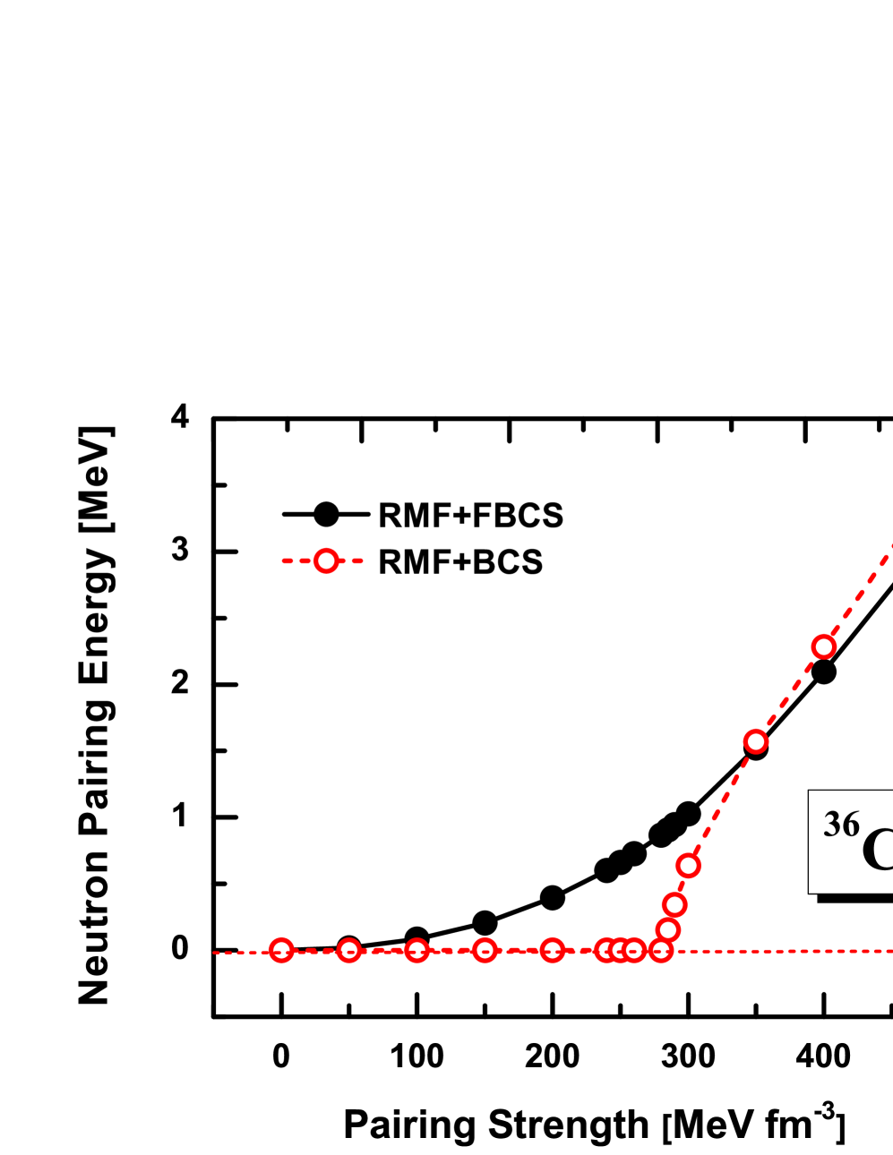
Figure 1: (Color online) Neutron pairing energy of ³⁶Ca as a function of the pairing strength.

Now we proceed to study the whole calcium isotopic chain from ³²Ca to ⁷⁴Ca. Two issues of particular interest are the magnitude of the pairing correlation and how it evolves as a function of the neutron (mass) number. One can define many different quantities for such a purpose P.Ring and P.Schuck (1980). Here we use the pairing energy defined in Eq. (17). In Fig. 2, we compare the neutron pairing energy of the calcium isotopes ^32-74Ca obtained from the RMF+FBCS and RMF+BCS calculations with pairing strengths $V_{0}=300$ MeV fm^-3 and $V_{0}=400$ MeV fm^-3, respectively. It is clear that the neutron pairing energies obtained with different pairing strengths show almost the same pattern. Particularly interesting is that at $N=14,20,28,32$ and 40, the neutron pairing energy is smaller than that of their neighbors in the RMF+FBCS model. The same scenario occurs in the RMF+BCS model except for $N=32$ with $V_{0}=300$ MeV fm^-3 where the pairing energy vanishes. This shows that not only the conventional magic numbers $N=20$, $28$, but also $N=14$, $40$, and to a less extent, $N=32$ shows some kind of “magicity”, which seems to agree with Refs Gade et al. (2006); Wienholtz et al. (2013); Grasso (2014); Li et al. (2016).

Figure 2: Neutron pairing energies of the calcium isotopes as a function of the neutron number with pairing strengths V₀=300 MeV fm^-3 and V₀=400 MeV fm^-3, respectively. The results from the RMF+FBCS model (empty columns) are compared with those from the RMF+BCS model (shaded columns).

Figure 3: Same as Fig. 2, but for the proton pairing energies.

In Fig. 3, we show the proton pairing energies of the calcium isotopes as a function of the neutron number. It can be seen that the RMF+FBCS pairing energies are still not zero, even for the proton magic number $Z=20$, which behave differently from those in the RMF+BCS calculations. Furthermore, the proton pairing energies vary lowly as a function of the neutron number, but the magnitude of this variation is small.

VI GROUND-STATE PROPERTIES OF CALCIUM ISOTOPES

In this section, we study how the bulk ground-state properties of the calcium isotopes can be described in the RMF+FBCS and RMF+BCS models. The pairing strength is fixed at $V_{0}=350$ MeV fm^-3 in the RMF+BCS model and that in the RMF+FBCS model is fixed at $V_{0}=274$ MeV fm^-3 by fitting to the odd-even mass differences of the whole calcium isotopic chain, defined as the following P.Ring and P.Schuck (1980); A.Bohr and Mottelson (1998):

$$\Delta^{(3)}(N,Z)=B(N-1,Z)-2B(N,Z)+B(N+1,Z).$$ (23)

Firstly, we examine the two-neutron separation energy defined as the following:

$$S_{2N}(Z,N)=B(Z,N)-B(Z,N-2),$$ (24)

where $B(Z,N)$ is the binding energy of a nucleus with proton number $Z$ and neutron number $N$. In the upper panel of Fig. 4, the two-neutron separation energies obtained from both models are compared with their experimental counterparts Huang et al. (2017). While in the lower panel, the deviations of the theoretical two neutron separation energies from their experimental counterparts are shown. One can easily see that except for $N=36$ and 38, the results of both methods agree with data quite well. It seems that the $N=40$ magicity effect is overestimated in the RMF model.

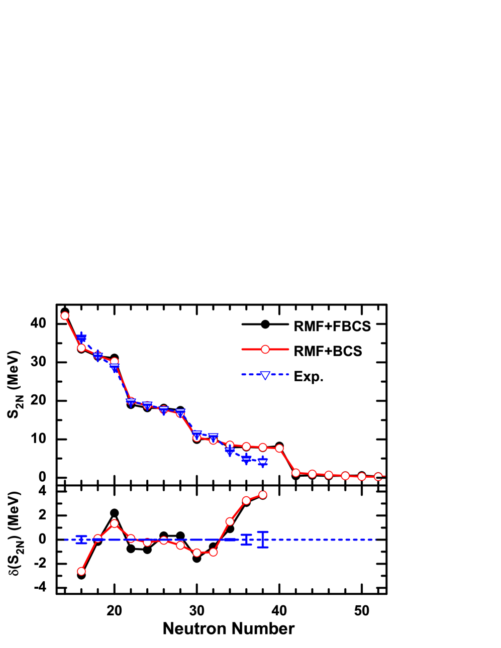
Figure 4: (Color online) Theoretical and experimental Huang et al. (2017) two-neutron separation energies S_2N of the calcium isotopes and the difference between them, defined as $\delta(S_{2N})$=$S_{2N}$(th)$-S_{2N}$(exp).

A closer look at the two-neutron separation energies of ⁴⁸Ca, ⁵⁰Ca, ⁵²Ca and ⁵⁴Ca in Fig. 5 reveals that the experimental sharp drop from ⁵²Ca to ⁵⁴Ca is better reproduced in the RMF+FBCS model. The same scenario is seen in the inset of Fig. 5 where there is a sharp drop from ⁷⁰Ca to ⁷²Ca in the RMF+FBCS model.

In Ref. Hinohara and Nazarewicz (2016), the pairing rotational moment of inertia is suggested to be an excellent pairing indicator, because odd-mass nuclei could contain the contribution from time-odd fields and better be avoided. The pairing rotational moment of inertia is proportional to the inverse of the two-nucleon shell gap indicator $\Delta_{2N}$ Lunney et al. (2003):

$$\Delta_{2N}(Z,N)=2B(Z,N)-B(Z,N+2)-B(Z,N-2)$$ (25)

In Fig. 6, the two-neutron shell gaps of the calcium isotopes and the deviations from their experimental counterparts are plotted as a function of the neutron number. It is seen that the RMF+BCS model provides a slightly better description of the experimental data, especially for ⁴⁰Ca and ⁴⁸Ca. This can be easily understood from the definition of $\Delta_{2N}$. In the BCS method the pairing correlation is only effective on open-shell nuclei and reduces the two-neutron shell gaps of magic nuclei (compared with pure mean field models or the FBCS method).

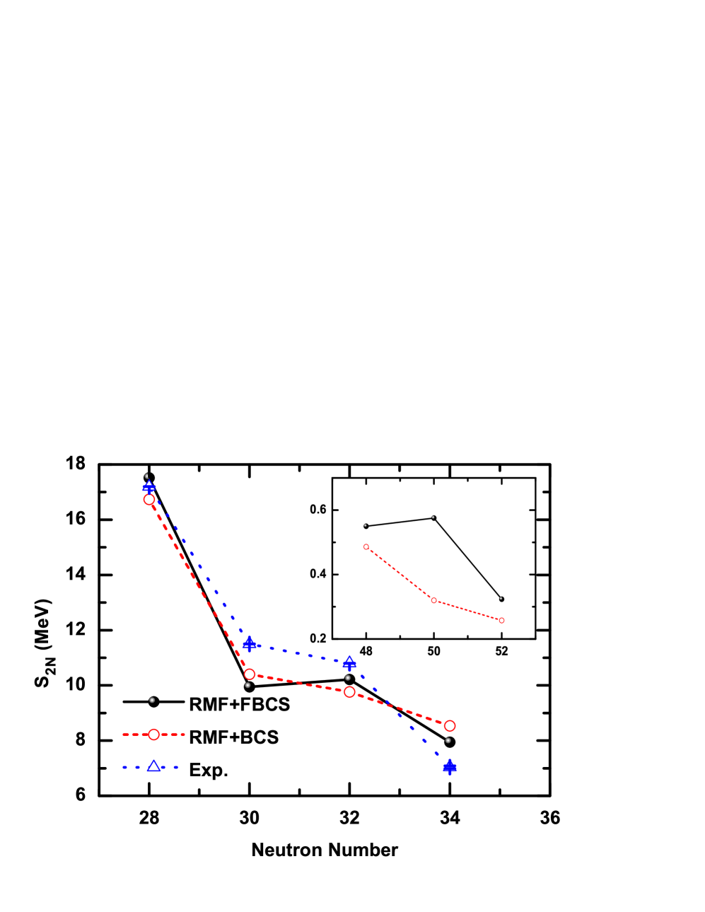
Figure 5: (Color online) Two-neutron separation energies of ⁴⁸Ca, ⁵⁰Ca, ⁵²Ca, and ⁵⁴Ca. The insert shows those of the ⁶⁸Ca, ⁷⁰Ca, and ⁷²Ca.

From the studies of the two-neutron separation energies and two-neutron gaps of the calcium isotopes, it seems that the RMF+BCS calculations are of similar quality or even slightly better than the RMF+FBCS calculations. This finding is not surprising. It is closely related to how we obtained the RMF parameters. The NL3 RMF parameterization is fitted to the ground-state properties of 10 magic or even-even nuclei Lalazissis et al. (1997). That is to say, from the very beginning, we only expect the residual pairing correlation to make open-shell nuclei more bound but leave closed-shell nuclei unchanged. The BCS and Bogoliubov methods are perfect candidates to achieve this as we can easily see in Fig. 3, though they break the gauge symmetry of particle number. In contrary, the FBCS method makes closed-shell nuclei more bound than what the BCS or Bogoliubov method does and leaves open-shell nuclei more or less unchanged. Therefore, it is quite natural that no significant improvement has been observed. To really appreciate the FBCS method, in particular to improve the agreement with the experimental data, the mean-field effective force has to be readjusted to leave room for incorporating these higher-order correlations Heenen et al. (2001). Due to the present strategy used to fit the RMF parameters, at least part of the pairing effect for magic nuclei has been compensated by artificially large magic number effects at the order of several MeV

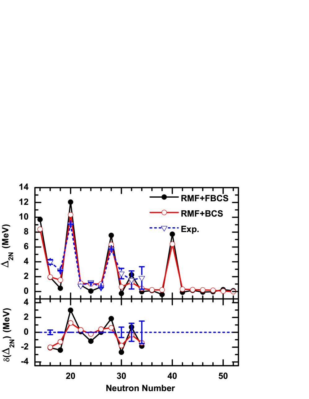
Figure 6: (Color online) Two-neutron gaps of the calcium isotopes and the differences between theoretical and experimental values Huang et al. (2017) as a function of the neutron number.

In addition to the binding energies and related quantities, one can study the root mean square (r.m.s.) radii as well as the deformations of the calcium isotopes. We found that they turn out to be similar in both the RMF+BCS and RMF+FBCS models and therefore refrain from showing them explicitly. On the other hand, we notice that close to the neutron drip line $N\geq 50$, the r.m.s. radii in the RMF+BCS model are slightly larger than those in the RMF+FBCS model, at the order of 0.05 fm. However, because of the harmonic oscillator basis adopted, we do not expect that either of our methods can properly describe the r.m.s. radii or the density distributions close to the neutron drip line. Nevertheless, we notice that the RMF+BCS and RMF+FBCS models can sometime change the occupation probability of certain single particle levels close to the Fermi surface, and thus modify the density distributions. When the continuum states are more properly treated, this may have some impact on the spatial distributions of drip line nuclei. To illustrate this point, we investigate ⁵⁴Ca in detail below.

In the upper panel of Fig. 7, we plot the potential energy surface of ⁵⁴Ca as a function of the quadrupole deformation parameter $\beta_{20}$. The curves obtained in the two models look quite similar, both yielding a minimum at $\beta_{20}=0$, but the RMF+FBCS energy at large deformations becomes larger. In the lower panel of Fig. 7, the neutron r.m.s. radius of ⁵⁴Ca is also shown as a function of $\beta_{20}$. Surprisingly, we see a bump developed in the center of the RMF+FBCS curve, different from the RMF+BCS case. 

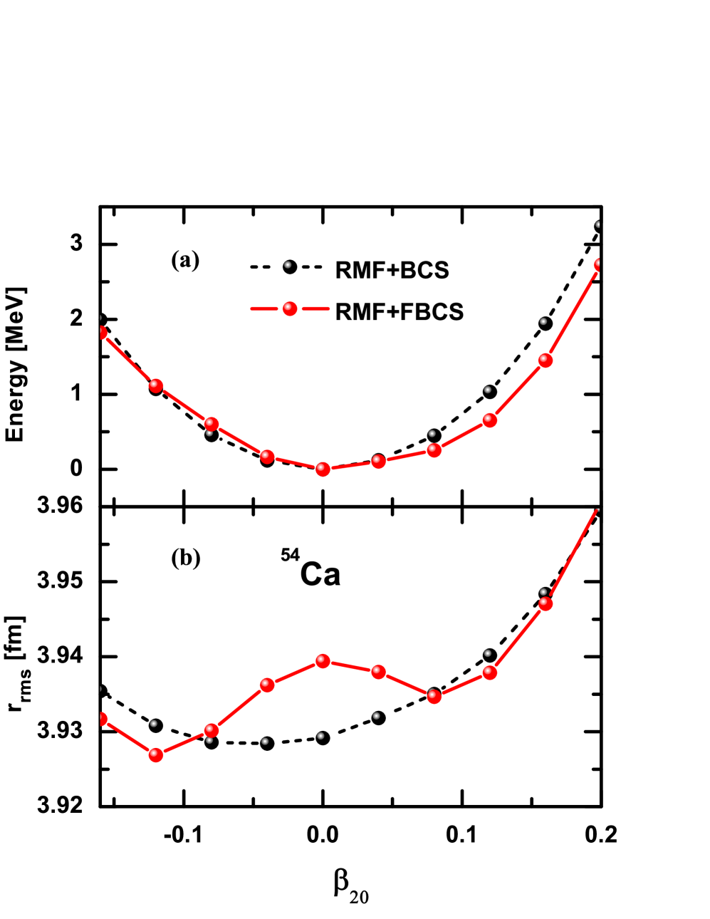
Figure 7: (Color online) Potential energy surface and root mean square radius of ⁵⁴Ca as a function of the deformation parameter $\beta_{20}$ obtained in the RMF+BCS (dashed line) model and the RMF+FBCS (solid line) model.

Since the binding energy at $\beta_{20}=0$ is similar to each other, such a difference can only originate from the different occupation probabilities of the single particle states close to the Fermi surface. This is indeed the case as shown in Fig. 8. We see that the occupation probability of the neutron $2p_{1/2}$ state in the RMF+ FBCS is much larger than that of the RMF+BCS model. In the latter, more particles are scattered to the neutron $1f_{5/2}$ orbit. This explains why at $\beta_{20}=0$, the RMF+BCS and RMF+FBCS models predict a similar binding energy, but a different neutron r.m.s. radius.

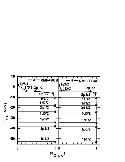
Figure 8: (Color online) Occupation probabilities of the neutron single particle levels of ⁵⁴Ca obtained in the RMF+BCS model (left) and the RMF+FBCS model (right).

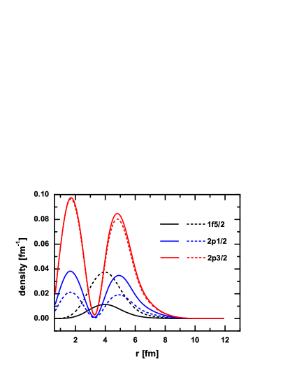
Figure 9: (Color online) Neutron density of the $1f_{5/2}$, $2p_{1/2}$, and $2p_{3/2}$ orbits of ⁵⁴Ca calculated in the RMF+FBCS (solid lines) and RMF+BCS (dashed lines) models.

In Fig. 9, we plot the density distributions of the neutron1f_5/2, 2p_1/2 and 2p_3/2 orbits. The Nilsson quantum numbers are those of the dominant component in the expansion of the wave function in terms of the axial harmonic oscillator basis. Clearly, in the two methods, the relative contributions from the $2p_{1/2}$ and $1f_{5/2}$ orbits are quite different. In the RMF+FBCS model, the contribution from the $2p_{1/2}$ orbit, which extends farther away from the center, is larger than that from the $1f_{5/2}$ orbit. While in the RMF+BCS model, the opposite is true. These are the reasons behind the seemingly unusual behavior observed in Fig. 8.

VII SUMMARY

We have formulated a particle number conserving BCS method, the so-called FBCS method, in the relativistic mean field model. It is shown the RMF+FBCS model can properly describe the weak pairing limit. A detailed study of the calcium isotopes reveals that the RMF+FBCS results for the two-neutron separation energies and two-neutron gaps are similar to those of the RMF+BCS calculations; and also the density distributions are roughly the same in both calculations (therefore not shown). Overall we do not find essential improvement in the description of the ground state properties of the calcium isotopes.

On the other hand, we notice that the neutron r.m.s radii at the neutron drip lines can be somewhat larger in the RMF+BCS model than in the RMF+FBCS model. In addition, our study showed that the FBCS method can change the occupation probability of certain single particle orbitals around the Fermi surface and therefore affect the neutron r.m.s radius. For the case of ⁵⁴Ca, the increase of the radius is only about 0.02 fm, but this can be larger for more neutron rich nuclei with similar configurations. However, due to the incorrect asymptotic behavior of the harmonic oscillator wave functions, the expansion in a localized HO basis is not appropriate for the description of drip line nuclei Zhou et al. (2003), particular for their density distributions. To treat the continuum more properly, one may solve the RMF model in coordinate space Sandulescu et al. (2003); Meng (1998) or adopt the Woods-Saxon basis  Zhou et al. (2003, 2010). Implementing a particle number conserving BCS approach or Bogoliubov approach in such models and study its impact on drip line nuclei is of great interest both experimentally and theoretically. Such works are in progress.