Asymptotic analysis of drug dissolution in two layers having widely differing diffusion coefficients

Abstract

This paper is concerned with a diffusion-controlled moving-boundary problem in drug dissolution, in which the moving front passes from one medium to another for which the diffusion coefficient is many orders of magnitude smaller. It has been shown in an earlier paper that a similarity solution exists while the front is passing through the first layer, but that this breaks down in the second layer. Asymptotic methods are used to understand what is happening in the second layer. Although this necessitates numerical computation, one interesting outcome is that only one calculation is required, no matter what the diffusion coefficient is for the second layer.

1 Introduction

Moving boundary problems arise in many industrial applications and, as a result, they have been studied extensively in the mathematical literature ([8, 2, 3]). When the problem is well characterised by a one-dimensional system of equations, analytical solutions are often readily obtained. For example, if the system comprises a one-dimensional diffusion equation with appropriate initial and boundary conditions, as well as a Stefan condition to track the position of the moving boundary, then it can often be shown that the problem is self-similar, and through a similarity reduction one may convert the original system to a system of ordinary differential equations. Some discussion of the analytical solution of moving boundary problems arising in diffusive systems can be found in [1].

However, it is not always the case that such a similarity structure exists for all time and often one has to resort to seeking a numerical solution using an appropriate numerical method: for example, a front-tracking finite difference scheme ([1]). In this context, a recent development, which is exploited in this work, is to analyze the governing partial differential equations for small time, determine if there is a similarity solution and, if there is, use it as an initial condition for the subsequent computation, which is performed in terms of the similarity variables, rather than the original physical variables; in particular, this approach is of importance for maintaining the accuracy of a numerical scheme in problems where the initial thickness of the domain of interest is zero ([5, 6, 7]), as will be the case in this work.

Whilst a common type of moving boundary problem often involves phase change, as in [5, 6, 7], an arguably less common type is where there is no phase change involved, but the front in question passes from one medium into another; in this situation also, there can be no hope of a similarity solution that is valid for all time. An example of an application where precisely this problem arises is presented in the recent publication by [9]; a particular characteristic of this problem is that the diffusion coefficient of the second medium is several orders of magnitude smaller than that of the first.

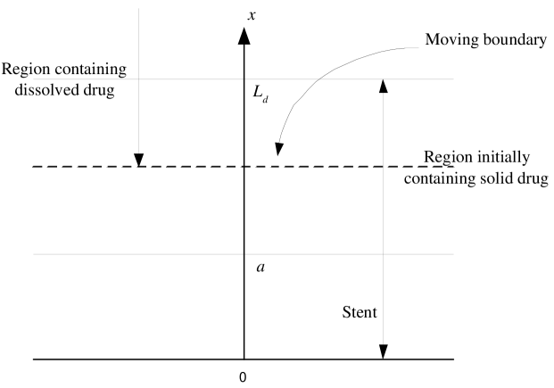
Figure 1: Schematic showing the problem considered by [9]. The region $0<x<L_{d}$ initially contains drug at uniform concentration $c_{0}$. For $t>0$, drug dissolves on a moving front (where the concentration is identically $c_{s}$, the solubility of the drug), starting at $x=L_{d}$. Drug dissolution is complete when the moving boundary tracks back to $x=0$. Dissolved drug diffuses out of the system into a release medium which is considered to be infinite. The diffusion coefficient of the dissolved drug in the region $0<x<a$ is much smaller than that in the region $x>a$.

[9] investigated the drug release from polymer-free coronary stents with microporous surfaces. The investigation was both experimental and theoretical. As part of the theoretical analysis, the following one-dimensional diffusion problem arose:

$$\frac{\partial c}{\partial t}=\frac{\partial}{\partial x}\left(D\left(x\right)\frac{\partial c}{\partial x}\right),\qquad x>s\left(t\right),\text{ }t>0,$$ (1.1)

$$c =c_{s},\quad-D\left(x\right)\frac{\partial c}{\partial x}=\frac{\mathrm{d}s}{\mathrm{d}t}(c_{s}-c_{0})\quad\text{at }x=s\left(t\right),t>0,$$ (1.2)

$$c \rightarrow 0\quad\text{as \ }x\rightarrow\infty,\text{ }t>0,$$ (1.3)

$$s\left(0\right)=L_{d},\quad c\left(x,0\right)=0\quad\text{for }x>L_{d}.$$ (1.4)

Here, $c$ represents the concentration of the drug, $s\left(t\right)$ a free surface between the dissolved and undissolved drug, $L_{d}$ denotes the thickness of the drug layer initially, which occupies the region $0<x<L_{d}$, $a<L_{d}$ denotes the mean position of the microporous region (also containing drug), $c_{s}$ the solubility of the drug and $c_{0}$ the initial constant concentration for $x<L_{d}.$ The spatially dependent diffusion coefficient is

$$D\left(x\right)=\left\{\begin{array}[c]{ll}D_{e}\left(<D_{w}\right)&\text{if }0<x\leq a_{-}\\ D_{w}&\text{if }x\geq a_{+}\end{array}\right..$$ (1.5)

The problem given by (1.1-1.5) gives rise to a two-stage release of drug (Figure 1). In Stage 1, the drug dissolves on a moving front in the region $a<x<L_{d}$ and diffuses out of the system. In Stage 2, the moving boundary has tracked back to $x=a$ and the drug then proceeds to dissolve from the rough surface region where it is released at a slower rate. For Stage 1 ($s\left(t\right)>a$), [9] wrote down an analytical solution, the derivation of which may be found in [4]. The solution is given by

$$s\left(t\right)=L_{d}-\theta\sqrt{t},\quad c\left(x,t\right)=\frac{c_{s}\text{erfc}\left(\frac{x-L_{d}}{2\sqrt{D_{w}t}}\right)}{\text{erfc}\left(-\frac{\theta}{2\sqrt{D_{w}}}\right)},\quad L_{d}-\theta\sqrt{t}<x<\infty,\text{ \ }0<t<t_{a},$$ (1.6)

where $\theta$ is determined by

$$\frac{\theta}{2\sqrt{D_{w}}}\exp\left(\frac{\theta^{2}}{4D_{w}}\right)\text{erfc}\left(-\frac{\theta}{2\sqrt{D_{w}}}\right)=\frac{1}{\sqrt{\pi}}\frac{c_{s}}{c_{0}-c_{s}}.$$ (1.7)

The solution is valid until $t=t_{a},$ whereupon $s\left(t_{a}\right)=a,$ so that

$$t_{a}=\frac{\left(L_{d}-a\right)^{2}}{\theta^{2}}.$$ (1.8)

Furthermore, at $t=t_{a},$

$$c\left(x,t_{a}\right)=c_{a}\left(x\right)=\frac{c_{s}\text{erfc}\left(\frac{x-L_{d}}{2\sqrt{D_{w}t_{a}}}\right)}{\text{erfc}\left(-\frac{\theta}{2\sqrt{D_{w}}}\right)},\quad a\leq x<\infty.$$ (1.9)

For Stage 2, a numerical procedure was employed.

In this paper, we will be concerned with the release of drug from the system during Stage 2. In particular, we adopt an asymptotic approach to derive approximate solutions for this phase of release. In Section 2, we start by presenting the equations that represent Stage 2 of the release. We then outline our asymptotic argument. In Section 3, we provide results including comparisons with the numerical solutions obtained by [9].

2 Stage 2 $\left(s\left(t\right)<a\right)$

The Stage 2 problem when $t>t_{a}$ may then be formulated in dimensional form as:

$$\frac{\partial c}{\partial t} =\frac{\partial}{\partial x}\left(D_{w}\frac{\partial c}{\partial x}\right),\qquad a<x<\infty,\quad t>t_{a},$$ (2.10)

$$\frac{\partial c}{\partial t} =\frac{\partial}{\partial x}\left(D_{e}\frac{\partial c}{\partial x}\right),\qquad s(t)<x<a,\quad t>t_{a},$$ (2.11)

$$c =c_{s},\quad-D_{e}\frac{\partial c}{\partial x}=\frac{\mathrm{d}s}{\mathrm{d}t}(c_{s}-c_{0}),\quad\text{at }x=s\left(t\right),$$ (2.12)

$$c \rightarrow 0,\quad\text{as }x\rightarrow\infty,$$ (2.13)

$$s\left(t_{a}\right) =a,\quad c\left(x,t_{a}\right)=c_{a}\left(x\right),\quad x\geq a.$$ (2.14)

In addition, we require

$$\left[c\right]_{-}^{+} =0\quad\text{at }x=a,$$ (2.15)

$$\left(D_{e}\frac{\partial c}{\partial x}\right)_{-} =\left(D_{w}\frac{\partial c}{\partial x}\right)_{+}\quad\text{at }x=a.$$ (2.16)

We non-dimensionalize the problem by setting

$$X=\frac{x}{a},\quad T=\frac{t-t_{a}}{a^{2}/D_{e}},\quad S=\frac{s}{a},\quad C=\frac{c}{c_{s}},\quad C_{a}=\frac{c_{a}}{c_{s}}.$$ (2.17)

This gives

$$\delta\frac{\partial C}{\partial T} =\frac{\partial^{2}C}{\partial X^{2}},\qquad 1<X<\infty,\quad T>0,$$ (2.18)

$$\frac{\partial C}{\partial T} =\frac{\partial^{2}C}{\partial X^{2}},\qquad S(T)<X<1,\quad T>0,$$ (2.19)

$$C =1,\quad-\frac{\partial C}{\partial X}=\frac{\mathrm{d}S}{\mathrm{d}T}(1-\frac{c_{0}}{c_{s}}),\quad\text{at }X=S\left(T\right),$$ (2.20)

$$C \rightarrow 0,\quad\text{as }X\rightarrow\infty,$$ (2.21)

$$S\left(0\right) =1,\quad C\left(X,0\right)=C_{a}\left(X\right),\quad X\geq 1,$$ (2.22)

where $\delta=D_{e}/D_{w}\ll 1,$ as in [9], and

$$C_{a}\left(X\right)=\frac{\text{erfc}\left(\frac{aX-L_{d}}{2\sqrt{D_{w}t_{a}}}\right)}{\text{erfc}\left(-\frac{\theta}{2\sqrt{D_{w}}}\right)}.$$ (2.23)

In addition, we have

$$\left[C\right]_{-}^{+} =0\quad\text{at }X=1,$$ (2.24)

$$\delta\left(\frac{\partial C}{\partial X}\right)_{-} =\left(\frac{\partial C}{\partial X}\right)_{+}\quad\text{at }X=1.$$ (2.25)

We have

$$\frac{\partial^{2}C}{\partial X^{2}} \approx 0,\quad 0<X<\infty,$$ (2.26)

$$C \rightarrow 0,\quad\text{as }X\rightarrow\infty,$$ (2.27)

$$\left(\frac{\partial C}{\partial X}\right)_{+} \approx\;0\quad\text{at }X=1,$$ (2.28)

which would require $C\equiv 0,$ for $X>1.$ For $X<1,$ we would have

$$\frac{\partial C}{\partial T} =\frac{\partial^{2}C}{\partial X^{2}},\qquad S(T)<X<1,\quad T>0,$$ (2.29)

$$C =1,\quad-\frac{\partial C}{\partial X}=\frac{\mathrm{d}S}{\mathrm{d}T}(1-\frac{c_{0}}{c_{s}}),\quad\text{at }X=S\left(T\right).$$ (2.30)

Also, (2.24) would imply

$$C=0\text{ at }X=1.$$

In fact, this cannot hold for all time, since $C=1$ at $X=1$ at $T=0,$ i.e. in dimensional form, $c=c_{s}$ when $x=s\left(t_{a}\right)=a.$

2.1 Asymptotic argument

The above suggests that we must try to retain the term on the left-hand side of (2.18), which can be achieved if $T\sim\delta.$ This will mean that the left-hand side of (2.19) will be large, and would need to be balanced by the right-hand side, indicating that $1-X,$ i.e. the width of the lower region, must be of an appropriately small width. Thus, we suppose that $1-X\sim\left[X\right],$ where $\left[X\right]\ll 1,$ and is still to be determined. Thus, with

$$1-X=\left[X\right]\tilde{X},\quad 1-S=\left[X\right]\tilde{S},\quad T=\delta\tilde{T},$$ (2.31)

we have

$$\frac{\partial C}{\partial\tilde{T}} =\frac{\partial^{2}C}{\partial X^{2}},\qquad 1<X<\infty,\quad\tilde{T}>0,$$ (2.32)

$$\frac{\left[X\right]^{2}}{\delta}\frac{\partial C}{\partial\tilde{T}} =\frac{\partial^{2}C}{\partial\tilde{X}^{2}},\qquad\tilde{X}>0,\quad\tilde{T}>0,$$ (2.33)

subject to

$$C \rightarrow 0\quad\text{as }X\rightarrow\infty,$$ (2.34)

$$C =1,\quad-\frac{\partial C}{\partial\tilde{X}}=\frac{\left[X\right]^{2}}{\delta}\frac{\mathrm{d}\tilde{S}}{\mathrm{d}\tilde{T}}(1-\frac{c_{0}}{c_{s}}),\quad\text{at }\tilde{X}=\tilde{S}\left(\tilde{T}\right),$$ (2.35)

$$\tilde{S} =0,\quad C=C_{a}\left(X\right),\quad\text{at }\tilde{T}=0,\text{ }X>1\left(\tilde{X}<0\right).$$ (2.36)

In addition, we have

$$\left[C\right]_{-}^{+} =0\quad\text{at }X=1,\left(\tilde{X}=0\right)$$ (2.37)

$$-\frac{\delta}{\left[X\right]}\left(\frac{\partial C}{\partial\tilde{X}}\right)_{\tilde{X}=0} =\left(\frac{\partial C}{\partial X}\right)_{X=1}.$$ (2.38)

We must now choose $\left[X\right]$ so that (2.32)-(2.38) constitute a self-consistent system. There are basically only two possibilities: $\left[X\right]\sim\delta$ and $\left[X\right]\sim\delta^{1/2}.$ We try these in turn.

2.1.1 $\left[X\right]\sim\delta$

Equation (2.33) gives

$$\frac{\partial^{2}C}{\partial\tilde{X}^{2}}=0,$$ (2.39)

subject to, from (2.35),

$$C=1,\quad\frac{\partial C}{\partial\tilde{X}}=0,\quad\text{at }\tilde{X}=\tilde{S}\left(\tilde{T}\right)$$ (2.40)

and

$$\left[C\right]_{-}^{+} =0\quad\text{at }X=1,$$ (2.41)

$$-\left(\frac{\partial C}{\partial\tilde{X}}\right)_{\tilde{X}=0} =\left(\frac{\partial C}{\partial X}\right)_{X=1}.$$ (2.42)

Thus, (2.39) and (2.40) give just $C\equiv 1$ for $X<1,$ which means that (2.41) and (2.42) would become

$$C =1\quad\text{at }X=1,$$ (2.43)

$$\left(\frac{\partial C}{\partial X}\right)_{X=1} =0.$$ (2.44)

Clearly what we have obtained is not self-consistent: $C$ for $X>1$ must satisfy two boundary conditions, (2.43) and (2.44), at $X=1,$ which is clearly not possible, and $\tilde{S}\left(\tilde{T}\right)$ remains undetermined.

2.1.2 $\left[X\right]\sim\delta^{1/2}$

With $\left[X\right]\sim\delta^{1/2},$ we have

$$\frac{\partial C}{\partial\tilde{T}}=\frac{\partial^{2}C}{\partial X^{2}},\qquad 1<X<\infty,\quad\tilde{T}>0,$$ (2.45)

subject to

$$C\rightarrow 0,\quad\text{as }X\rightarrow\infty,$$ (2.46)

and, from (2.38),

$$\frac{\partial C}{\partial X}=0\quad\text{at }X=1.$$ (2.47)

Also, (2.33) becomes

$$\frac{\partial C}{\partial\tilde{T}}=\frac{\partial^{2}C}{\partial\tilde{X}^{2}},\qquad\tilde{X}>0,\quad\tilde{T}>0,$$ (2.48)

subject to

$$C =C_{+}\left(\tilde{T}\right)\quad\text{at }\tilde{X}=0,$$ (2.49)

$$C =1,\quad-\frac{\partial C}{\partial\tilde{X}}=\frac{\mathrm{d}\tilde{S}}{\mathrm{d}\tilde{T}}(1-\frac{c_{0}}{c_{s}}),\quad\text{at }\tilde{X}=\tilde{S}\left(\tilde{T}\right),$$ (2.50)

where

$$C_{+}\left(\tilde{T}\right)=C\left(X=1_{+},\tilde{T}\right).$$ (2.51)

Note that $C_{+}\left(0\right)=1,$ i.e. $c\left(a,t_{a}\right)=c_{s}.$

We observe that the problem for $X>1$ (i.e. $x>a$) decouples from that for $X<1$ ($x<a$); we now solve these in turn.

2.2 $X\geq 1$

First, we solve the problem for $X\geq 1,\tilde{T}\geq 0,$ corresponding to $x\geq a,t\geq t_{a}.$ From Section 2.1.2, the problem at hand is

$$\frac{\partial C}{\partial\tilde{T}}=\frac{\partial^{2}C}{\partial X^{2}},$$ (2.52)

subject to

$$\frac{\partial C}{\partial X} =0\quad\text{at }X=1,$$ (2.53)

$$C \rightarrow 0\quad\text{as }X\rightarrow\infty,$$ (2.54)

$$C =C_{a}\left(X\right)\quad\text{at }\tilde{T}=0,$$ (2.55)

Setting $\xi=X-1,$ we have

$$\frac{\partial C}{\partial\tilde{T}}=\frac{\partial^{2}C}{\partial\xi^{2}},$$ (2.56)

subject to

$$\frac{\partial C}{\partial\xi} =0\quad\text{at }\xi=0,$$ (2.57)

$$C \rightarrow 0\quad\text{as }\xi\rightarrow\infty,$$ (2.58)

$$C =C_{a}\left(\xi\right)\quad\text{at }\tilde{T}=0,$$ (2.59)

where

$$C_{a}\left(\xi\right)=\frac{\text{erfc}\left(\frac{a\left(1+\xi\right)-L_{d}}{2\sqrt{D_{w}t_{a}}}\right)}{\text{erfc}\left(-\frac{\theta}{2\sqrt{D_{w}}}\right)}.$$ (2.60)

Thence, using Fourier transforms, we obtain

$$C\left(\xi,\tilde{T}\right)=\frac{1}{2\sqrt{\pi\tilde{T}}}\int_{0}^{\infty}C_{a}\left(X^{\prime}\right)\left\{\exp\left(-\frac{\left(\xi-X^{\prime}\right)^{2}}{4\tilde{T}}\right)+\exp\left(-\frac{\left(\xi+X^{\prime}\right)^{2}}{4\tilde{T}}\right)\right\}\mathrm{d}X^{\prime}.$$ (2.61)

Before we can tackle the second problem (i.e. the case $X<1),$ we shall require $C_{+}\left(\tilde{T}\right)=C\left(\xi=0,\tilde{T}\right)$ for condition (2.49), i.e.

$$C_{+}\left(\tilde{T}\right)=\frac{1}{\sqrt{\pi\tilde{T}}}\int_{0}^{\infty}C_{a}\left(X^{\prime}\right)\exp\left(-\frac{X^{\prime^{2}}}{4\tilde{T}}\right)\mathrm{d}X^{\prime}.$$ (2.62)

Putting $z=X^{\prime}/2\sqrt{\tilde{T}},$ we have

$$C_{+}\left(\tilde{T}\right) =\frac{2}{\sqrt{\pi}}\int_{0}^{\infty}C_{a}\left(2z\sqrt{\tilde{T}}\right)e^{-z^{2}}\mathrm{d}z$$

$$=C_{a}\left(0\right)+\frac{2\sqrt{\tilde{T}}}{\sqrt{\pi}}\frac{\mathrm{d}C_{a}}{\mathrm{d}\xi}\left(0\right)+O\left(\tilde{T}\right),$$ (2.63)

where we have used a Taylor series expansion for $C_{a}$ about $z=0.$ Now, on using (2.60) and recalling equation (1.8), we note that $C_{a}\left(0\right)=1$ and that

$$\frac{\mathrm{d}C_{a}}{\mathrm{d}\xi}\left(0\right)=-\frac{a}{\sqrt{\pi D_{w}t_{a}}}\frac{\text{exp}\left(-\frac{\left(a-L_{d}\right)^{2}}{4D_{w}t_{a}}\right)}{\text{erfc}\left(-\frac{\theta}{2\sqrt{D_{w}}}\right)}.$$

So, we have, for small $\tilde{T},$

$$C_{+}\left(\tilde{T}\right)=1-\left\{\frac{2a}{\pi\sqrt{D_{w}t_{a}}}\frac{\text{exp}\left(-\frac{\left(a-L_{d}\right)^{2}}{4D_{w}t_{a}}\right)}{\text{erfc}\left(-\frac{\theta}{2\sqrt{D_{w}}}\right)}\right\}\sqrt{\tilde{T}}+O\left(\tilde{T}\right).$$ (2.64)

However, to determine $C\left(0,\tilde{T}\right)$ for all $\tilde{T},$ we need to revert to (2.62) with $z=X^{\prime}/2\sqrt{\tilde{T}},$ which gives

$$C_{+}\left(\tilde{T}\right)=\frac{2}{\sqrt{\pi}\text{erfc}\left(-\frac{\theta}{2\sqrt{D_{w}}}\right)}\int_{0}^{\infty}\text{erfc}\left(f\left(z,\tilde{T}\right)\right)e^{-z^{2}}\mathrm{d}z,$$ (2.65)

where

$$f\left(z,\tilde{T}\right)=\frac{a\left(1+2z\sqrt{\tilde{T}}\right)-L_{d}}{2\sqrt{D_{w}t_{a}}}.$$

Differentiating with respect to $\tilde{T},$ we have

$$\frac{\mathrm{d}C_{+}}{\mathrm{d}\tilde{T}}=-\frac{2a}{\pi\text{erfc}\left(-\frac{\theta}{2\sqrt{D_{w}}}\right)\sqrt{D_{w}t_{a}\tilde{T}}}\int_{0}^{\infty}ze^{-\left(z^{2}+f^{2}\left(z,\tilde{T}\right)\right)}\mathrm{d}z.$$ (2.66)

Rearranging the argument in the exponential in (2.66), we have

$$z^{2}+\frac{\left(2az\sqrt{\tilde{T}}+a-L_{d}\right)^{2}}{4D_{w}t_{a}}=\mathcal{A}\left(\tilde{T}\right)\left\{\left(z+\mathcal{B}\left(\tilde{T}\right)\right)^{2}+\mathcal{C}\left(\tilde{T}\right)\right\},$$

where

$$\mathcal{A}\left(\tilde{T}\right) =1+\frac{a^{2}\tilde{T}}{D_{w}t_{a}},$$ (2.67)

$$\mathcal{B}\left(\tilde{T}\right) =\frac{\left[\frac{\left(a-L_{d}\right)a\sqrt{\tilde{T}}}{D_{w}t_{a}}\right]}{2\left(1+\frac{a^{2}\tilde{T}}{D_{w}t_{a}}\right)},$$ (2.68)

$$\mathcal{C}\left(\tilde{T}\right) =\frac{\frac{\left(a-L_{d}\right)^{2}}{4D_{w}t_{a}}}{\left(1+\frac{a^{2}\tilde{T}}{D_{w}t_{a}}\right)}-\frac{\left[\frac{\left(a-L_{d}\right)a\sqrt{\tilde{T}}}{D_{w}t_{a}}\right]^{2}}{4\left(1+\frac{a^{2}\tilde{T}}{D_{w}t_{a}}\right)^{2}};$$ (2.69)

it is now possible to write the integral in (2.66) in the form

$$\int_{0}^{\infty}ze^{-\left\{\mathcal{A}\left(\tilde{T}\right)\left[\left(z+\mathcal{B}\left(\tilde{T}\right)\right)^{2}+\mathcal{C}\left(\tilde{T}\right)\right]\right\}}\mathrm{d}z.$$ (2.70)

Next, with $\zeta=z+\mathcal{B}\left(\tilde{T}\right)$ and later $\xi=\mathcal{A}^{1/2}\left(\tilde{T}\right)\zeta,$ we have

$$\int_{0}^{\infty}ze^{-\mathcal{A}\left(\tilde{T}\right)\left[\left(z+\mathcal{B}\left(\tilde{T}\right)\right)^{2}+\mathcal{C}\left(\tilde{T}\right)\right]}\mathrm{d}z$$

$$=\frac{1}{2}e^{-\mathcal{A}\left(\tilde{T}\right)\mathcal{C}\left(\tilde{T}\right)}\left\{\frac{e^{-\mathcal{A}\left(\tilde{T}\right)\mathcal{B}^{2}\left(\tilde{T}\right)}}{\mathcal{A}\left(\tilde{T}\right)}-\frac{\pi^{1/2}\mathcal{B}\left(\tilde{T}\right)}{\mathcal{A}^{1/2}\left(\tilde{T}\right)}\text{erfc}\left(\mathcal{A}^{1/2}\left(\tilde{T}\right)\mathcal{B}\left(\tilde{T}\right)\right)\right\}.$$ (2.71)

Hence, we have the following first-order ordinary differential equation (ODE) for $C_{+}\left(\tilde{T}\right):$

$$\frac{\mathrm{d}C_{+}}{\mathrm{d}\tilde{T}}=-\frac{ae^{-\mathcal{A}\left(\tilde{T}\right)\mathcal{C}\left(\tilde{T}\right)}}{\pi\text{erfc}\left(-\frac{\theta}{2\sqrt{D_{w}}}\right)\sqrt{D_{w}t_{a}}\sqrt{\tilde{T}}}\left\{\frac{e^{-\mathcal{A}\left(\tilde{T}\right)\mathcal{B}^{2}\left(\tilde{T}\right)}}{\mathcal{A}\left(\tilde{T}\right)}-\frac{\pi^{1/2}\mathcal{B}\left(\tilde{T}\right)}{\mathcal{A}^{1/2}\left(\tilde{T}\right)}\text{erfc}\left(\mathcal{A}^{1/2}\left(\tilde{T}\right)\mathcal{B}\left(\tilde{T}\right)\right)\right\},$$ (2.72)

subject to

$$C_{+}=1\quad\text{at }\tilde{T}=0.$$ (2.73)

Checking $\mathcal{A}\left(\tilde{T}\right),\mathcal{B}\left(\tilde{T}\right),\mathcal{C}\left(\tilde{T}\right)$ in the limit as $\tilde{T}\rightarrow 0,$ we have

$$\mathcal{A}\left(0\right)=1,\quad\mathcal{B}\left(0\right)=0,\quad\mathcal{C}\left(0\right)=\frac{\left(a-L_{d}\right)^{2}}{4D_{w}t_{a}},$$ (2.74)

so that

$$\frac{\mathrm{d}C_{+}}{\mathrm{d}\tilde{T}}\sim\left(-\frac{ae^{-\left(a-L_{d}\right)^{2}/4D_{w}t_{a}}}{\pi\text{erfc}\left(-\frac{\theta}{2\sqrt{D_{w}}}\right)\sqrt{D_{w}t_{a}}}\right)\frac{1}{\sqrt{\tilde{T}}}.$$ (2.75)

2.3 $X<1$

For this region, we require to solve (2.48)-(2.51). Note that, from the solution for $X>1,$ we have already found in (2.64) that, for small $\tilde{T},$

$$C_{+}\left(\tilde{T}\right)-1\sim\tilde{T}^{1/2}.$$ (2.76)

Moreover, at $\tilde{T}=0,$ the region that we are solving in, i.e. $0<\tilde{X}<\tilde{S}\left(\tilde{T}\right),$ has zero width, which suggests that it may be appropriate to proceed in terms of similarity or similarity-like variables. For this purpose, we set

$$C-1=\tilde{T}^{1/2}F\left(\eta,\tilde{T}\right),\qquad\eta=\frac{\tilde{X}}{\tilde{S}\left(\tilde{T}\right)},$$ (2.77)

so that equation (2.48) becomes

$$\frac{\tilde{S}^{2}\left(\tilde{T}\right)F}{2\tilde{T}}+\left(\tilde{S}^{2}\left(\tilde{T}\right)\frac{\partial F}{\partial\tilde{T}}-\tilde{S}\left(\tilde{T}\right)\frac{\mathrm{d}\tilde{S}}{\mathrm{d}\tilde{T}}\eta\frac{\partial F}{\partial\eta}\right)=\frac{\partial^{2}F}{\partial\eta^{2}},$$ (2.78)

subject to

$$1+\tilde{T}^{1/2}F =C_{+}\left(\tilde{T}\right)\quad\text{at }\eta=0,$$ (2.79)

$$F =0\quad\text{at }\eta=1,$$ (2.80)

$$-\frac{\partial F}{\partial\eta} =\frac{\tilde{S}\left(\tilde{T}\right)}{\tilde{T}^{1/2}}\frac{\mathrm{d}\tilde{S}}{\mathrm{d}\tilde{T}}(1-\frac{c_{0}}{c_{s}})\quad\text{at }\eta=1.$$ (2.81)

It is now required that (2.78)-(2.81) behave in a self-consistent manner as $\tilde{T}\rightarrow 0;$ by this, we mean that we should obtain an ODE, subject to the requisite number of boundary conditions.

To consider this systematically, start with equation (2.78) and suppose that we try to retain as many terms on the left-hand side as possible as $\tilde{T}\rightarrow 0;$ this can be done if

$$\tilde{S}\left(\tilde{T}\right)\frac{\mathrm{d}\tilde{S}}{\mathrm{d}\tilde{T}}\sim 1,$$ (2.82)

which implies that $\tilde{S}\sim\tilde{T}^{1/2}$ and there is clearly a sensible balance of leading order terms in (2.78) as $\tilde{T}\rightarrow 0$. However, the right-hand side of equation (2.81) would become unbounded as $\tilde{T}\rightarrow 0,$ and hence (2.82) does not lead to overall self-consistency in this limit. Note also that if we try with

$$\tilde{S}\left(\tilde{T}\right)\frac{\mathrm{d}\tilde{S}}{\mathrm{d}\tilde{T}}\gg 1,$$

instead of (2.82), then the left-hand side of (2.78) dominates the right-hand side, and it will not be possible to satisfy all of the boundary conditions as $\tilde{T}\rightarrow 0.$ The only remaining possibility is if

$$\tilde{S}\left(\tilde{T}\right)\frac{\mathrm{d}\tilde{S}}{\mathrm{d}\tilde{T}}\ll 1.$$ (2.83)

To pin the behaviour down more precisely, we turn to (2.81), which suggests that

$$\frac{\tilde{S}\left(\tilde{T}\right)}{\tilde{T}^{1/2}}\frac{\mathrm{d}\tilde{S}}{\mathrm{d}\tilde{T}}\sim 1,$$ (2.84)

in order to balance with the term on the left-hand side. In this case, we obtain $\tilde{S}\left(\tilde{T}\right)\sim\tilde{T}^{3/4},$ which ensures a sensible leading-order balance in (2.78) and (2.81), noting also that (2.83) is fulfilled, since

$$\tilde{S}\left(\tilde{T}\right)\frac{\mathrm{d}\tilde{S}}{\mathrm{d}\tilde{T}}\sim\tilde{T}^{1/2}.$$

Setting $\tilde{S}\left(\tilde{T}\right)=\lambda\tilde{T}^{3/4}+..,$ where $\lambda$ is a positive constant to be determined, equation (2.78) becomes, in the limit as $\tilde{T}\rightarrow 0,$

$$\frac{\mathrm{d}^{2}F_{0}}{\mathrm{d}\eta^{2}}=0,$$ (2.85)

where

$$F_{0}\left(\eta\right):=\lim_{\tilde{T}\rightarrow 0}F\left(\eta,\tilde{T}\right).$$ (2.86)

subject to

$$F_{0} =\mu\quad\text{at }\eta=0,$$ (2.87)

$$F_{0} =0\quad\text{at }\eta=1,$$ (2.88)

$$-\frac{\mathrm{d}F_{0}}{\mathrm{d}\eta} =\frac{3}{4}\lambda^{2}(1-\frac{c_{0}}{c_{s}})\quad\text{at }\eta=1,$$ (2.89)

where $\mu$ is a constant given by

$$\mu=\lim_{\tilde{T}\rightarrow 0}\frac{\left(C\right)_{X=1}-1}{\tilde{T}^{1/2}}.$$ (2.90)

Note that $\mu$ can be determined, and we will do so shortly, from the solution for $X>1.$ Thus, solving (2.85) subject to (2.87)-(2.89) gives

$$F_{0}\left(\eta\right)=\mu\left(1-\eta\right),$$ (2.91)

with

$$\mu=\frac{3}{4}\lambda^{2}(1-\frac{c_{0}}{c_{s}}),$$ (2.92)

i.e.

$$\lambda=\pm\left(\frac{4\mu}{3(1-c_{0}/c_{s})}\right)^{1/2}.$$ (2.93)

Clearly, we need to take the positive sign to ensure that $\tilde{S}$ increases, i.e. $S$ decreases. Also, since $c_{0}>c_{s},$ it is clear that we will need $\mu<0;$ we return to this point shortly.

Note also that it is possible to determine $\mu$ without solving (2.52)-(2.55). Near $X=1,$ we have

$$C_{a}=1+\left(X-1\right)\left(\frac{\mathrm{d}C_{a}}{\mathrm{d}X}\right)_{X=1}+...$$ (2.94)

Now,

$$C_{a}\left(X\right)=\frac{1+\text{erf}\left(\frac{L_{d}-aX}{2\sqrt{D_{w}t_{a}}}\right)}{\text{erfc}\left(-\frac{\theta}{2\sqrt{D_{w}}}\right)},$$ (2.95)

whence

$$\alpha:=\left(\frac{\mathrm{d}C_{a}}{\mathrm{d}X}\right)_{X=1}=-\frac{a\exp\left(-\frac{\left(L_{d}-a\right)^{2}}{4D_{w}t_{a}}\right)}{\sqrt{\pi D_{w}t_{a}}\text{erfc}\left(-\frac{\theta}{2\sqrt{D_{w}}}\right)}.$$ (2.96)

We consider the small and positive $X-1$ and small $\tilde{T}$ behaviour of (2.52)-(2.55) by setting $\xi=X-1,$ as after (2.55), and

$$C=1+\tilde{T}^{1/2}G\left(\zeta,\tilde{T}\right),\quad\zeta=\xi/\tilde{T}^{1/2}.$$ (2.97)

Equation (2.52) becomes

$$\tilde{T}\frac{\partial G}{\partial\tilde{T}}+\frac{G}{2}-\frac{\zeta}{2}\frac{\partial G}{\partial\zeta}=\frac{\partial^{2}G}{\partial\zeta^{2}}.$$ (2.98)

Now, in the limit as $\tilde{T}\rightarrow 0,$ (2.98) becomes

$$\frac{G_{0}}{2}-\frac{\zeta}{2}\frac{\mathrm{d}G_{0}}{\mathrm{d}\zeta}=\frac{\mathrm{d}^{2}G_{0}}{\mathrm{d}\zeta^{2}},$$ (2.99)

where

$$G_{0}\left(\zeta\right):=\lim_{\tilde{T}\rightarrow 0}G\left(\zeta,\tilde{T}\right).$$ (2.100)

Equation (2.99) has the general solution

$$G_{0}=K_{1}\zeta+K_{2}\left(\pi\zeta\operatorname{erf}\left(\frac{\zeta}{2}\right)+2\sqrt{\pi}\exp\left(-\frac{\zeta^{2}}{4}\right)\right),$$ (2.101)

where $K_{1}$ and $K_{2}$ are constants to be determined. Clearly, (2.99) must have two boundary conditions. One of these comes from (2.53), and is

$$\frac{\mathrm{d}G_{0}}{\mathrm{d}\zeta}=0\quad\text{at }\zeta=0.$$ (2.102)

The other comes from matching $G_{0}$ as $\zeta\rightarrow\infty$ to $C_{a}$ and is

$$\frac{\mathrm{d}G_{0}}{\mathrm{d}\zeta}\rightarrow\alpha\quad\text{as }\zeta\rightarrow\infty.$$ (2.103)

Since

$$\frac{\mathrm{d}G_{0}}{\mathrm{d}\zeta}=K_{1}+K_{2}\pi\operatorname{erf}\left(\frac{\zeta}{2}\right),$$ (2.104)

we quickly see that

$$K_{1}=0,\quad K_{2}=\frac{\alpha}{\pi},$$ (2.105)

whence

$$G_{0}=\alpha\left(\zeta\operatorname{erf}\left(\frac{\zeta}{2}\right)+\frac{2}{\sqrt{\pi}}\exp\left(-\frac{\zeta^{2}}{4}\right)\right);$$ (2.106)

ultimately, this leads to

$$\mu=G_{0}\left(0\right)=\frac{2\alpha}{\pi^{1/2}}.$$ (2.107)

Finally, recall from the discussion after equation (2.93) that we needed $\mu<0.$ Now, equation (2.107) implies that we will need $\alpha<0;$ from equation (2.96), we see that this will clearly be the case.

3 Results

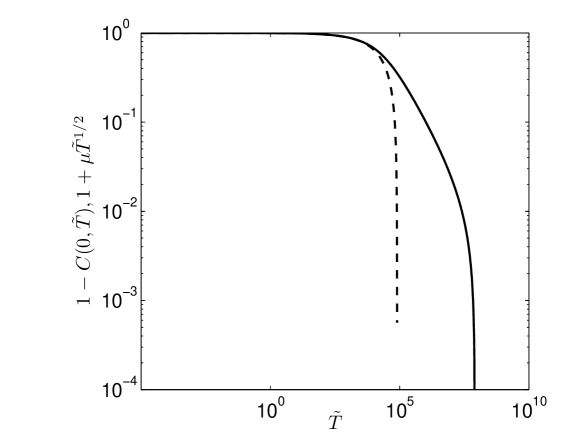
Figure 2: $1-C\left(0,\tilde{T}\right)$ (solid line) and $1+\mu\tilde{T}^{1/2}$ (dashed line) vs. $\tilde{T}$

The main numerical task is to solve equation (2.78), subject to (2.79)-(2.81); this constitutes a moving boundary problem for $F$ and $\tilde{S}.$ However, (2.79) contains $C_{+}\left(\tilde{T}\right),$ which must itself be solved for numerically via the first-order ODE (2.72), subject to (2.73). To illustrate our ideas, we will vary the value of $D_{e},$ so as to see the effect of $\delta,$and select the following parameters from [9]: $L_{d}=10^{-5}$ m, $a=0.2L_{d},$ $D_{w}=5\times 10^{-11}$ m²s${}^{-1},$ $c_{0}/c_{s}=50.$

However, before presenting the results, we note first that we are ultimately interested in determining the time at which the front reaches $x=0;$ this corresponds to the time at which $\tilde{S}=1/\delta^{1/2}.$ Whilst this will, of course, depend on the value of $\delta,$ we observe that $c_{s}-c\left(a,t\right),$ and hence $1-C\left(\tilde{X}=0,\tilde{T}\right),$ i.e. $1-C_{+}\left(\tilde{T}\right)$, will be independent of $\delta;$ this is evident since there is no $\delta$ in either equation (2.72) or (2.73). Thus, it makes sense to look at $1-C\left(0,\tilde{T}\right)$ vs. $\tilde{T},$ ahead of considering the solutions for $\tilde{S}$ and $C\left(X,\tilde{T}\right).$ Thus, Fig. 2 shows a log-log plot for $1-C\left(0,\tilde{T}\right)$ vs. $\tilde{T},$ as well $1+\mu\tilde{T}^{1/2}$ vs. $\tilde{T};$ the second of these is the small-time approximation for $1-C\left(0,\tilde{T}\right)$ derived in Section 2.3 and makes use of the form for $C$ in (2.97) and (2.107). We see that this approximation works quite well until $\tilde{T}\sim 10^{4},$ after which the two curves diverge.

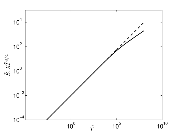
Figure 3: $\tilde{S}$ (solid line, computed) and $\lambda\tilde{T}^{3/4}$ (dashed line) vs. $\tilde{T}.$ Note that the computation has been stopped at $\tilde{T}=10^{8};$ at this stage $\tilde{S}$ $\approx 9823,$ which implies that $\delta\approx 10^{-8}.$ In more detail, with $\bar{S}=1/\delta^{1/2},$ we have $\delta=1/9823^{2}=$ 1.0364$\times 10^{-8}.$

Next, Fig. 3 shows $\tilde{S}$ vs. $\tilde{T},$ as well as $\lambda\tilde{T}^{3/4}$ vs. $\tilde{T};$ the latter of these is also from the small-time approximation, as indicated between equations (2.84) and (2.85). Whilst this result does not depend on $\delta$ either$,\$we have stopped the computation when $\tilde{S}$ reaches $O\left(10^{4}\right)$, with a view to exploring the results when $\delta\geq 10^{-8};$ this covers the range in $\delta$ considered in [9]. Here also, we see that the two curves follow each other until $\tilde{T}\sim 10^{4},$ at which point $\tilde{S}\sim 10^{2}$. This would mean that, for 10${}^{-4}\leq\delta\ll 1,$ a preliminary estimate for $\tilde{T}$ of when $\tilde{S}=1/\delta^{1/2},$ which we denote by $\tilde{T}_{stop},$ would be given by

$$\lambda\tilde{T}_{stop}^{3/4}\approx\frac{1}{\delta^{1/2}},$$ (3.108)

giving $\tilde{T}_{stop}\approx\left(\lambda\delta^{1/2}\right)^{-4/3}.$ In actual time, this amounts to

$$t_{stop}:=a^{2}\delta\tilde{T}_{stop}/D_{e}\left(=a^{2}\tilde{T}_{stop}/D_{w}\right),$$ (3.109)

where $t_{stop}$ is the time taken for the front to move from $X=1$ to $X=0,$ i.e. $x=a$ to $x=0.$

However, the values for $\delta$ used in [9] lie outside of this range - they are smaller - and any attempt to use equation (3.108) can thus be expected to underestimate the value of $t_{stop}.$ Instead, in Table 1, we compare the values of $t_{stop}$ as given by the solid line in Fig. 3, which were obtained from the solution of (2.78)-(2.81), and as estimated from Fig. 3 in [9], for different values of $\delta$. As can be seen, the qualitative and quantitative agreement is very good.

$\delta$	$t_{stop}\left[\text{days}\right]$
	Fig. 3	[9]
$5\times 10^{-7}$	$\sim$46.4	$\sim$46.5
$10^{-6}$	$\sim$23.8	$\sim$23
$5\times 10^{-6}$	$\sim$4.97	$\sim$5
$10^{-5}$	$\sim$2.6	$\sim$2.5

Table 1: $t_{stop},$ as calculated in two different ways for four values of $\delta.$

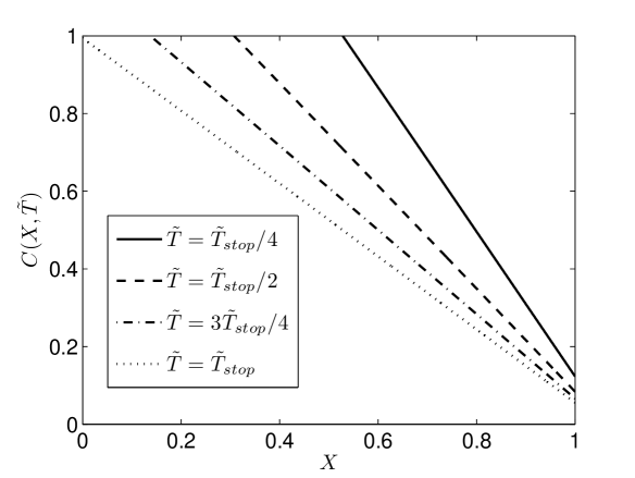
Figure 4: $C$ vs. $X$ for four different values of $\tilde{T}$ for $\delta=10^{-5}$ .  $\tilde{T}_{stop}$ corresponds to $t_{stop}=$2.6 days.

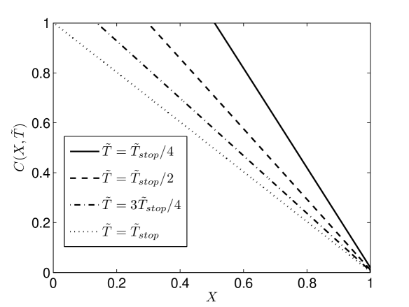
Figure 5: $C$ vs. $X$ for four different values of $\tilde{T}$ for $\delta=5\times 10^{-7}$ .  $\tilde{T}_{stop}$ corresponds to $t_{stop}=$46.4 days.

An interesting observation now arises: if $D_{w},$ $L_{d}/a$ and $c_{0}/c_{s}$ are fixed, only one computation, i.e. the one that was already carried out to determine the profile for $\tilde{S}$ for $\tilde{T}$ as great as 10⁸ already and which generated the results for Fig. 3, is required to find the solution for $C\left(X,\tilde{T}\right),$ which comes from the solution for $F$ via equation (2.77), for any value of $\delta!$ This is as opposed to having to carry out a new computation on each occasion that $D_{e},$ and hence $\delta,$ is changed, as was done in [9]. To see this, we show in Figs. 4 and 5 $C$ as a function of $X$ for $\tilde{S}\left(\tilde{T}\right)\leq X\leq 1$ for four different values of $\tilde{T}$ for $\delta=10^{-5}$ and 5$\times$10${}^{-7},$ respectively; note that, in these figures, the concentration profile at $\tilde{T}=0,$ corresponding to $t=t_{a},$ consists of a point that is located at $C=1$ and $X=1$ but which then become a curve - a line, as it turns out - that moves down and to the left with time. In both figures, $X$ is related to the independent variables of the domain in which the computations were carried out, $\eta$ and $\tilde{T},$ by

$$X=1-\delta^{1/2}\eta\tilde{S}\left(\tilde{T}\right),$$

as can be seen by tracking back through the substitutions in equations (2.17), (2.31) and (2.77).

References

- [1] J. Crank. Free and moving boundary problems. New York: Oxford University Press Inc., 1984.
- [2] E. Hansen and P. Hougaard. On a moving boundary problem from biomechanics. IMA J. Appl. Maths, 13:385–398, 1974.
- [3] F. Liu and D. McElwain. A computationally efficient solution technique for moving-boundary problems in finite media. IMA J. Appl. Maths, 59:71–84, 1997.
- [4] S. McGinty, T. T. N. Vo, M. Meere, S. McKee, and C. McCormick. Some design considerations for polymer-free drug-eluting stents: A mathematical approach. Acta Biomaterialia, 18:213–225, 2015.
- [5] S. L. Mitchell and M. Vynnycky. Finite-difference methods with increased accuracy and correct initialization for one-dimensional Stefan problems. Appl. Math. Comp., 215:1609–1621, 2009.
- [6] S. L. Mitchell and M. Vynnycky. On the numerical solution of two-phase Stefan problems with heat-flux boundary conditions. J. Comp. Appl. Maths, 264:49–64, 2014.
- [7] S. L. Mitchell and M. Vynnycky. On the accurate numerical solution of a two-phase Stefan problem with phase formation and depletion. J. Comp. Appl. Maths, 300:259–274, 2016.
- [8] R. D. Passo and P. D. Mottoni. On a moving boundary problem aristing in fluidized bed combustion. IMA J. Appl. Maths, 43:101–126, 1989.
- [9] T. T. N. Vo, S. Morgan, C. McCormick, S. McGinty, S. McKee, and M. Meere. Modelling drug release from polymer-free coronary stents with microporous surfaces. Accepted for publication in Int. J. Pharm. DOI:10.1016/j.ijpharm.2017.12.007, 2018.