Driven particle flux through a membrane: Two-scale asymptotics of a diffusion equation with polynomial drift

Abstract

Diffusion of particles through an heterogenous obstacle line is modeled as a two-dimensional diffusion problem with a one–directional nonlinear convective drift and is examined using two-scale asymptotic analysis. At the scale where the structure of heterogeneities is observable the obstacle line has an inherent thickness. Assuming the heterogeneity to be made of an array of periodically arranged microstructures (e.g. impenetrable solid rectangles), two scaling regimes are identified: the characteristic size of the microstructure is either significantly smaller than the thickness of the obstacle line or it is of the same order of magnitude. We scale up the convection-diffusion model and compute the effective diffusion and drift tensorial coefficients for both scaling regimes. The upscaling procedure combines ideas of two-scale asymptotics homogenization with dimension reduction arguments. Consequences of these results for the construction of more general transmission boundary conditions are discussed. We numerically illustrate the behavior of the upscaled membrane in the finite thickness regime and apply it to describe the transport of CO₂ through paperboard.

MSC Classification: 35B27, 76M50, 76M45,

Keywords: convection-diffusion, upscaling, dimension reduction, derivation of transmission boundary conditions

Appunti:

1 Introduction

The study of the physics of interfaces has known a great impulse in the last decades [23], mainly motivated by the study of surfaces separating two different phases. Interface fluctuations, controlled by surface tension, have been studied with the methods of statistical mechanics, in particular those borrowed from the theory of equilibrium critical phenomena. Membrane–like interfaces, namely, surfaces made of a different kind of molecules with respect to those forming the medium, do not need to separate regions of space filled with different phases, but they exhibit wide fluctuations, too, due to the smallness of their surface tension. In particular, depending on the temperature, they can undergo a phase transition between a flat and a crumpled phase [4].

In this paper we investigate flat static (not fluctuating) membranes separating two regions of space and crossed by a fluid. This is the typical setup one is interested in when studying membrane filtration. Traditionally, membrane filtration is one of the most common methods for purifying fluids; see e.g. [17] and references cited therein. Furthermore, recent advances in conductive and mass transport through a composite medium have led to increased interest in the process of mixed-matrix membrane separation. In such cases, small particles of a microporous material, identified as a filler, are dispersed in a dense nonporous polymer material, identified as a matrix, and then processed into a thin composite layer, identified as a membrane. The objective is that the filler, chosen for its high adsorption affinity or transport rate for a molecular species of interest, improves the efficacy of the matrix in membrane-mediated separation [26]. Depending on pore sizes and level of microscopic activity, one also encounters the so-called enhanced matrix diffusion [28].

Our main motivation is to develop multiscale mathematical modelling strategies of transport processes that can describe, over several space scales, how internal structural features of the filler and local defects affect the permeability of the material, perceived as a thin long permeable membrane. As concrete applications we have in mind the transport of O₂ and CO₂ molecules through packaging materials (paperboard) as well as the dynamics of human crowds through barrier-like heterogeneous environments (active particles walking inside geometries with obstacles).

We study the diffusion of particles through such a thin heterogeneous membrane under a one–directional nonlinear drift. Using the mean–field equation

$$\frac{\partial u}{\partial t}-d_{1}\frac{\partial^{2}u}{\partial x_{1}^{2}}-d_{2}\frac{\partial^{2}u}{\partial x_{2}^{2}}=-b\frac{\partial}{\partial x_{1}}[u(1-u)]+f(x),$$ (1.1)

with $b>0$, which is found in the hydrodynamic limit of the two–dimensional random walk with simple exclusion and drift along the $x_{1}$-direction (for details, see [5]), we study the possibility to upscale the system and to compute the effective transport coefficients accounting for the presence of the membrane, adding analytic results to our simulation study [6].

In [5, 6] the same problem is addressed in a microscopic setup. A lattice model, known as simple exclusion model, is considered on a two–dimensional strip of $\mathbb{Z}^{2}$. There, particles move randomly on the strip with the constraint that at most one particle at a time can occupy the sites of the lattice. Particles move choosing at random one of the four neighboring sites and a drift is introduced in the dynamics so that one of the four direction is possibly more probable. This model is a generalization of the celebrated TASEP (total asymmetric simple exclusion model) which is a one–dimensional simple exclusion model in which particles move to the right at random times [10].

In this framework, the equation (1.1) is derived in the macroscopic diffusive limit, i.e., when the space and the drift are rescaled with a small parameter and, correspondingly, the time is rescaled with the square of the same parameter. In [5] we have reported a useful heuristic derivation of this equation which, in the one–dimensional case, was rigorously proven in [11] (see, also, [20] for an account of the more recent techniques developed in the framework of hydrodynamic limit theory). In particular, this heuristic computation shows that the two diffusion coefficients can be different as a consequence of the fact that at the microscopic level the probability of a particle to move horizontally or vertically can differ. Moreover, and this is much more important in our context, the peculiar structure of the transport term on the right hand side is related to the probability of a particle performing a move, which the simple exclusion might prevent. Consequently, the factor $u$ comes from the probability to find a particle at a given site and the factor $1-u$ accounts for the probability that the site where the particle tries to move to is indeed empty. Thus, we can summarize this discussion saying that the peculiar form of the right hand side of equation (1.1) is, at the microscopic level, connected to the hard–core repulsion of the molecules.

We stress that the model we have in mind is (1.1), but the techniques that will be developed in this article will apply to a much more general transport term obtained by substituting $u(1-u)$ with a general polynomial in terms of $u$.

For a special scaling regime, we perform a simultaneous homogenization asymptotics and dimension reduction, allowing us not only to replace the heterogeneous membrane by an homogeneous obstacle line, but also to provide the effective transmission conditions needed to complete the upscaled model equations. The heterogeneities we account for in this context are assumed to be arranged periodically, but the same methodology can be adapted to cover also the locally periodic case. Additionally, we investigate also the effect of diffusion correlations and cross-diffusion (diagonal vs. full diffusion tensors) on the structure of the upscaled equations. We observe that in the case of the infinitely thin upscaled membrane the structure of the limit equations is unchanged, while in the case of the finite-length upscaled membrane the presence of the off-diagonal terms does not permit the use of closed form representations of oscillations in terms of cell functions. Furthermore, it is worth mentioning that the clogging of the membrane cannot be achieved with our model. Local clogging can eventually be reached by allowing the boundaries of the microstructures to evolve freely. As working techniques, we employ scaling arguments as well as two-scale homogenization asymptotic expansions to guess the structure of the model equations and the corresponding effective transport coefficients. As a long term plan, we would like to see whether infinitely-thin periodic membrane models can be used to give insight in the nonlinear structure of localized singularities arising in reaction terms connected to quenching structures; see for instance the settings from [8] and [9]. The question here is what a microscopic membrane would model look like so that it gives rise to production terms by reaction of the form $\eta(r,s)=k\frac{r}{s^{\gamma}}$ in a certain asymptotic regime, where $k>0,0<\gamma\leq 1$ for $r,s\in[0,\infty]$ for coupled systems of semi-linear reaction-diffusion equations (cf. [7]).

The research presented in this article pursues a formal asymptotics route; it follows the thread of the original mathematical analysis work by M. Neuss-Radu and W. Jäger in [24] by adding to the discussion the presence of nonlinear transport terms and is remotely related to our work on filtration combustion through heterogeneous thin layers; compare [19]. Recent follow-up (mathematical analysis) works of [24] are reported in [2, 15, 16] (where the authors apply the concept of two-scale boundary layer convergence to the corresponding setting). Strongly connected scenarios to the transport-through-membranes problem are the theoretical estimation of the effective interfacial resistance of regular rough surfaces (cf- [12], e.g.) and the upscaling of reaction, diffusion, and flow processes in porous media with thin fissures (cf. [3, 27], e.g.).

What makes our study peculiar and innovative is the combination of the heterogeneous structure of the space region where particles move and the presence of the transport term on the right-hand side in the evolution equation (1.1). Indeed, our results extend to a more general model assuming the transport term to be the $x_{1}$-derivative of a polynomial of the field $u$ with a finite arbitrary large degree. The main finding of this study can be summarized as follows:

• We deduced the structure of the formal asymptotic expansions which are behind the concept of two-scale boundary layer convergence from [24]; this structure can be further employed to construct corrector estimates to justify the upscaling and to provide convergence rates.

• We derived the structure of the upscaled transmission conditions across the obstacle line with the corresponding jumps in both transport fluxes and concentrations expressed in terms of the (local) physics taking place inside the microstructures (heterogeneities) of the membrane.

• Using finite element approximations of our model equations implemented in FEniCS ([1]), we numerically illustrate the behavior of the upscaled membrane in the finite thickness regime. We simulate the basic membrane scenario using a reference parameter set corresponding to the penetration of gaseous CO₂ through a porous paper sheet. This gives confidence that our model equations and their implementation can be used in practical applications and, in principle, can be extended to cover more complex membrane microstructures than the locally periodic regime.

The article is organized as follows: In Section 2 we present the equations of our mean-field model as well as the membrane geometry. After a suitable scaling, we point out two relevant asymptotic regimes in terms of a small parameter $\varepsilon$ which incorporates the periodicity and selected size effects of the internal structure of the membrane. Section 3 contains the derivation of the finite thickness upscaled membrane model, while in Section 4 we consider the more delicate case of the upscaling of the infinitely-thin membrane. Here the two-scale homogenization asymptotics is performed simultaneously with a dimension reduction procedure – a non-standard singular perturbation problem. We numerically illustrate in Section 5 the behavior of the upscaled membrane in the finite thickness regime. Finally, in Section 6 we present our conclusions.

2 The model

Let $\ell,h>0$ and consider the two–dimensional strip $[-\ell/2,\ell/2]\times[0,h]$, say that $\ell$ and $h$ are, respectively, its horizontal and vertical side lengths. Partition the strip into the blocks $\omega_{\textrm{l}}=[-\ell/2,-w/2]\times[0,h]$, $\omega_{\textrm{m}}=[-w/2,w/2]\times[0,h]$, $\omega_{\textrm{r}}=[w/2,\ell/2]\times[0,h]$, and call $\omega_{\textrm{m}}$ the membrane. Let $0<\eta\leq h$ and $\varepsilon=2\eta/\ell$. We partition the membrane into rectangular cells $\omega_{\textrm{c}}^{i}=(-w/2,w/2)\times((i-1)\eta,i\eta)\cap(0,h)$ with $i$ running from one to the smallest integer larger than or equal to $h/\eta$. In each cell consider an impenetrable disk, called obstacle, with center in the center of the cell and diameter $O(\varepsilon)$ in the limit $\varepsilon\to 0$. Denote by $\omega_{\textrm{o}}$ the union of all the obstacles.

We denote by $\gamma_{\textrm{v}}$ and $\gamma_{\textrm{h}}$, the vertical and horizontal boundaries of the strip, by $\gamma_{\textrm{o}}$ the boundary of the obstacle region $\omega_{\textrm{o}}$ and by $\gamma_{\textrm{i}}$ the boundary of the region $\omega_{\textrm{i}}$ for $\textrm{i}=\textrm{l,m,r}$. The external normal direction to a closed curve is denoted here by $n$.

Figure 2.1: Schematic representation of the model geometry.

We let $\omega=(\omega_{\textrm{l}}\cup\omega_{\textrm{r}}\cup\omega_{\textrm{m}})\setminus\omega_{\textrm{o}}$ and $f:\omega\to{\mathbb{R}}$ be a real function. Fixing the parameters $d_{1},d_{2}>0$, we consider the differential problem

$$\frac{\partial u}{\partial t}-d_{1}\frac{\partial^{2}u}{\partial x_{1}^{2}}-d_{2}\frac{\partial^{2}u}{\partial x_{2}^{2}}=-\frac{\partial}{\partial x_{1}}bu(1-u)+f(x)\quad\mbox{in}\,\,\omega,$$ (2.2)

endowed with the homogeneous Neumann boundary conditions

$$\Big{(}d_{1}\frac{\partial u}{\partial x_{1}}-bu(1-u),d_{2}\frac{\partial u}{\partial x_{2}}\Big{)}\cdot n=0\;\;\;\textrm{ on }\gamma_{\textrm{h}}\cup\gamma_{\textrm{o}},$$ (2.3)

as well as with the Dirichlet conditions

$$u(x,t)=u_{\textrm{l}}\;\;\textrm{ on }\gamma_{\textrm{v}}\cap\gamma_{\textrm{l}}\;\;\textrm{ and }\;\;u(x,t)=u_{\textrm{r}}\;\;\textrm{ on }\gamma_{\textrm{v}}\cap\gamma_{\textrm{r}}$$ (2.4)

for any $t\geq 0$, where $u_{\textrm{l}},u_{\textrm{r}}\in{\mathbb{R}}$. As initial condition we take

$$u(x,0)=v(x)\;\;\textrm{ on }\omega.$$ (2.5)

2.1 The non–dimensional model

It is useful to introduce dimensionless variables

$$X=(X_{1},X_{2})=\Big{(}\frac{2x_{1}}{\ell},\frac{2x_{2}}{\ell}\Big{)}\;\;\textrm{ and }\;\;T=\frac{t}{\tau},\;$$ (2.6)

where $\tau$ is a fixed positive real.

Using (2.6), the original strip is mapped to $[-1,1]\times[0,2h/\ell]$, which is partitioned into $\Omega_{\textrm{l}}=[-1,-w/\ell]\times[0,2h/\ell]$, $\Omega_{\textrm{m}}=[-w/\ell,w/\ell]\times[0,2h/\ell]$, and $\Omega_{\textrm{r}}=[w/\ell,1]\times[0,2h/\ell]$. The cells are mapped to $\Omega_{\textrm{c}}^{i}=(-w/\ell,w/\ell)\times((i-1)\varepsilon,i\varepsilon)\cap(0,2h/\ell)$, where we recall that $\varepsilon=2\eta/\ell$. In the new variables, we denote by $\Omega_{\textrm{o}}$ the region occupied by the obstacle and by $\Gamma_{\textrm{v}}$, $\Gamma_{\textrm{h}}$, $\Gamma_{\textrm{l}}$, $\Gamma_{\textrm{m}}$, $\Gamma_{\textrm{r}}$, and $\Gamma_{\textrm{o}}$ the boundaries introduced above.

Figure 2.2: Schematic representation of the dimensionless model geometry.

It is convenient to set

$$U(X,T)=u\Big{(}\frac{\ell X}{2},\tau T\Big{)},\;V(X)=v\Big{(}\frac{\ell X}{2}\Big{)},\;F(X)=\tau f\Big{(}\frac{\ell X_{1}}{2},\frac{\ell X_{2}}{2}\Big{)}$$ (2.7)

and rewrite the model (2.2) as follows

$$\frac{\partial U}{\partial T}+\nabla\cdot J=F$$ (2.8)

in $\Omega=(\Omega_{\textrm{l}}\cup\Omega_{\textrm{r}}\cup\Omega_{\textrm{m}})\setminus\Omega_{\textrm{o}}$, where we introduced the flux

$$J=-D(\nabla U+G(U))\;,$$ (2.9)

with the derivatives in $\nabla$ taken with respect to the dimensionless variables $X_{1},X_{2}$, and let

$$D=\left(\begin{array}[]{cc}D_{1}&0\\ 0&D_{2}\end{array}\right),\;D_{1}=\frac{4\tau d_{1}}{\ell^{2}},\;D_{2}=\frac{4\tau d_{2}}{\ell^{2}},\;\textrm{ and }\;G(U)=\left(\begin{array}[]{c}g(U)\\ 0\end{array}\right),\;\;$$ (2.10)

with $g(U)=\ell p(U)/(2d_{1})$, where $p(U)=-bU(1-U)$ – a choice that makes (2.9) to correspond precisely to the setting discussed in [6].

The derivations done in this paper cover the more general case:

$$D=\left(\begin{array}[]{cc}D_{11}&D_{12}\\ D_{21}&D_{22}\end{array}\right),\;\;G(U)=\left(\begin{array}[]{c}g(U)\\ 0\end{array}\right),\;\;\textrm{ and }\;p(U)\textrm{ an arbitrary polynomial}.$$ (2.11)

To fix ideas, we take $p(U)=\sum_{n=1}^{k}a_{n}U^{n}$, where $a_{n}\in\mathbb{R}$. If not mentioned otherwise, in the rest of the paper $D$ is a full matrix as indicated in (2.11).

For any $T\geq 0$, problem (2.8) is endowed with the Dirichlet boundary conditions

$$U(X,T)=u_{\textrm{l}}\;\;\textrm{ on }\Gamma_{\textrm{v}}\cap\Gamma_{\textrm{l}}\;\;\textrm{ and }\;\;U(X,T)=u_{\textrm{r}}\;\;\textrm{ on }\Gamma_{\textrm{v}}\cap\Gamma_{\textrm{r}},$$ (2.12)

the Neumann boundary conditions

$$J\cdot n=0\quad\mbox{on}\,\,\Gamma_{\textrm{h}}\cup\Gamma_{\textrm{o}},$$ (2.13)

and the initial condition

$$U(X,0)=V(X)\;\;\textrm{ in }\Omega.$$ (2.14)

3 Derivation of the finite-thickness upscaled membrane model

In this section, we use a two-scale homogenization approach to average the membrane’s internal structure and then to derive the corresponding upscaled equation for the mass transport as well as the effective transport coefficient. If the diffusion matrix is diagonal, then we point out explicitly the structure of the corresponding tortuosity tensor.

3.1 Two-scale expansions

We look for effective equations in the limit in which the height of the cells tends to zero and its number is increased so that the total height of the cells equals that of the whole strip. Due to the periodic micro–structure of the membrane $\Omega_{\textrm{m}}$, with vertical spatial period $\varepsilon=2\eta/\ell$, it is reasonable to attack the problem expanding the unknown function $U$ in the membrane region as

$$U(X,T)=\sum_{n=0}^{\infty}\varepsilon^{n}U^{\textrm{m}}_{n}(X,Y_{2},T)\;\;\;\;\;\;\;\textrm{in }\Omega_{\textrm{m}},$$ (3.15)

where $Y_{2}=X_{2}/\varepsilon$ and the functions $U^{\textrm{m}}_{n}$ are $Y_{2}-$periodic functions.

By abusing slightly the notation, we understand in (2.8)

$$\nabla=\nabla_{X}+\frac{1}{\varepsilon}\nabla_{Y_{2}}\;\;\textrm{with }\nabla_{X}=\left(\begin{array}[]{c}\frac{\partial}{\partial X_{1}}\\ \frac{\partial}{\partial X_{2}}\end{array}\right)\;\;\textrm{and }\nabla_{Y_{2}}=\left(\begin{array}[]{c}0\\ \frac{\partial}{\partial Y_{2}}\end{array}\right)\;.$$

We now compute the various terms appearing in (2.8) in the different regions of $\Omega$. We have

$$\frac{\partial U}{\partial T}=\sum_{n=0}^{\infty}\varepsilon^{n}\frac{\partial U^{\textrm{m}}_{n}}{\partial T}\;\;\textrm{ and }\;\;\frac{\partial U}{\partial X_{1}}=\sum_{n=0}^{\infty}\varepsilon^{n}\frac{\partial U^{\textrm{m}}_{n}}{\partial X_{1}}\;\;\;\;\;\;\;\textrm{ in }\Omega_{\textrm{m}}.$$ (3.16)

For handling the terms involving the gradient $\nabla$, we have to distinguish the regions $\Omega_{\textrm{l}}$, $\Omega_{\textrm{m}}$, and $\Omega_{\textrm{r}}$. In $\Omega_{\textrm{l}}$ and $\Omega_{\textrm{r}}$ we simply have $\nabla U(X,T)=\nabla U_{0}^{l}(X,T)$ in $\Omega_{l}$ and $\nabla U(X,T)=\nabla U_{0}^{r}(X,T)$ in $\Omega_{r}$. Instead of $\nabla U_{0}^{l}$ and $\nabla U_{0}^{r}$, we will use $\nabla U^{l}$ and $\nabla U^{r}$, respectively.

In $\Omega_{\textrm{m}}$, the computation of the gradient reads

$$\begin{split}\nabla U=&\nabla\sum_{n=0}^{\infty}\varepsilon^{n}U^{\textrm{m}}_{n}=\sum_{n=0}^{\infty}\varepsilon^{n}\nabla_{X}U^{\textrm{m}}_{n}+\sum_{n=0}^{\infty}\varepsilon^{n}\frac{1}{\varepsilon}\nabla_{Y_{2}}U^{\textrm{m}}_{n}\\ =&\frac{1}{\varepsilon}\nabla_{Y_{2}}U^{\textrm{m}}_{0}+\sum_{n=0}^{\infty}\varepsilon^{n}(\nabla_{X}U^{\textrm{m}}_{n}+\nabla_{Y_{2}}U^{\textrm{m}}_{n+1}).\\ \end{split}$$ (3.17)

Hence, it yields

$$\begin{array}[]{rcl}\nabla\cdot D\nabla U&\!\!=&\!\!{\displaystyle\frac{1}{\varepsilon^{2}}\nabla_{Y_{2}}\cdot D\nabla_{Y_{2}}U^{\textrm{m}}_{0}+\frac{1}{\varepsilon}\nabla_{X}\cdot D\nabla_{Y_{2}}U^{\textrm{m}}_{0}}\\ &\!\!&\!\!{\displaystyle+\sum_{n=0}^{\infty}\varepsilon^{n}\Big{[}\nabla_{X}\cdot D\nabla_{X}U^{\textrm{m}}_{n}+\nabla_{X}\cdot D\nabla_{Y_{2}}U^{\textrm{m}}_{n+1}+\frac{1}{\varepsilon}\nabla_{Y_{2}}\cdot D\nabla_{X}U^{\textrm{m}}_{n}}\\ &\!\!&\!\!{\displaystyle\phantom{+\sum_{n=0}^{\infty}\varepsilon^{n}\Big{[}}+\frac{1}{\varepsilon}\nabla_{Y_{2}}\cdot D\nabla_{Y_{2}}U^{\textrm{m}}_{n+1}\Big{]}}\\ &\!\!=&\!\!{\displaystyle\frac{1}{\varepsilon^{2}}\nabla_{Y_{2}}\cdot D\nabla_{Y_{2}}U^{\textrm{m}}_{0}+\frac{1}{\varepsilon}[\nabla_{X}\cdot D\nabla_{Y_{2}}U^{\textrm{m}}_{0}+\nabla_{Y_{2}}\cdot D\nabla_{X}U^{\textrm{m}}_{0}}\\ &\!\!&\!\!{\displaystyle\phantom{\frac{1}{\varepsilon^{2}}\nabla_{Y_{2}}\cdot D\nabla_{Y_{2}}U^{\textrm{m}}_{0}+\frac{1}{\varepsilon}[}+\nabla_{Y_{2}}\cdot D\nabla_{Y_{2}}U^{\textrm{m}}_{1}]}\\ &\!\!&\!\!{\displaystyle+\sum_{n=0}^{\infty}\varepsilon^{n}[\nabla_{X}\cdot D\nabla_{X}U^{\textrm{m}}_{n}+\nabla_{X}\cdot D\nabla_{Y_{2}}U^{\textrm{m}}_{n+1}+\nabla_{Y_{2}}\cdot D\nabla_{X}U^{\textrm{m}}_{n+1}}\\ &\!\!&\!\!{\displaystyle\phantom{+\sum_{n=0}^{\infty}\varepsilon^{n}[}+\nabla_{Y_{2}}\cdot D\nabla_{Y_{2}}U^{\textrm{m}}_{n+2}].}\end{array}$$ (3.18)

Moreover, we have

$$DG(U)=\left(\begin{array}[]{c}D_{1}g(U)\\ 0\\ \end{array}\right)=DG(U^{\textrm{m}}_{0})+\varepsilon D\left(\begin{array}[]{c}U^{\textrm{m}}_{1}\sum_{n=1}^{k}nb_{n}(U^{\textrm{m}}_{0})^{n-1}\\ 0\\ \end{array}\right)+o(\varepsilon).$$ (3.19)

It is worth noting already at this stage that if the matrix $D$ is diagonal, then (3.19) reduces to

$$\nabla\cdot DG(U)=\nabla_{X}\cdot DG(U^{\textrm{m}}_{0})+o(1)\;\;.$$ (3.20)

We consider now the equation inside the membrane region $\Omega_{\textrm{m}}$ at the lowest order $\varepsilon^{-2}$ and we find

$$\nabla_{Y_{2}}\cdot D\nabla_{Y_{2}}U^{\textrm{m}}_{0}=0.$$ (3.21)

By expanding $J$ and by collecting the lowest $\varepsilon$ order, we get the Neumann boundary condition

$$(-D\nabla_{Y_{2}}U^{\textrm{m}}_{0})\cdot n=0\quad\mbox{on}\,\,(\Gamma_{\textrm{o}}\cup\Gamma_{\textrm{h}})\cap\Omega_{\textrm{m}}$$ (3.22)

and the following transmission boundary conditions:

$$U^{\textrm{m}}_{0}(X,T)=U^{\textrm{l}}_{0}(X,T)\quad\mbox{on}\,\,\Gamma_{\textrm{l}}\cap\Gamma_{\textrm{m}}\;\;\textrm{ and }\;\;U^{\textrm{m}}_{0}(X,T)=U^{\textrm{r}}_{0}(X,T)\quad\mbox{on}\,\,\Gamma_{\textrm{r}}\cap\Gamma_{\textrm{m}}$$

as well as

$$-D(\nabla U^{\textrm{l}}+G(U^{\textrm{l}}))\cdot n=-D(\nabla U^{\textrm{m}}_{0}+G(U^{\textrm{m}}_{0}))\mbox{ at }\Gamma_{\textrm{l}}\cap\Gamma_{\textrm{m}},$$ (3.23)

$$-D(\nabla U^{\textrm{r}}+G(U^{\textrm{r}}))\cdot n=-D(\nabla U^{\textrm{m}}_{0}+G(U^{\textrm{m}}_{0}))\mbox{ at }\Gamma_{\textrm{r}}\cap\Gamma_{\textrm{m}},$$ (3.24)

for any $T\geq 0$.

We recall that $U^{\textrm{m}}_{0}$ is $Y_{2}-$periodic. Based on (3.21) and (3.22), we claim that $U^{\textrm{m}}_{0}$ is independent of $Y_{2}$, i.e. $U^{\textrm{m}}_{0}=U^{\textrm{m}}_{0}(X,T)$.

At the order $\varepsilon^{-1}$, using that $U^{\textrm{m}}_{0}$ does not depend on $Y_{2}$, we get the equation

$$\nabla_{Y_{2}}\cdot D\nabla_{Y_{2}}U^{\textrm{m}}_{1}=-\nabla_{Y_{2}}\cdot D\nabla_{X}U^{\textrm{m}}_{0}$$ (3.25)

with Neumann boundary condition (2.13) at order $\varepsilon^{0}$ in (3.17) and (3.19)

$$-D\nabla_{Y_{2}}U^{\textrm{m}}_{1}\cdot n=D\nabla_{X}U^{\textrm{m}}_{0}\cdot n+DG(U^{\textrm{m}}_{0})\cdot n\mbox{ on }\Gamma_{h}\cup\Gamma_{o}.$$ (3.26)

Recall that $U^{\textrm{m}}_{1}$ is $Y_{2}-$periodic.

3.2 $D$ diagonal matrix

If $D$ is a diagonal matrix, then the structure of (3.25) allows us to assume that

$$U^{\textrm{m}}_{1}=W(Y_{2})\cdot\left[\nabla_{X}U^{\textrm{m}}_{0}+G(U^{\textrm{m}}_{0})\right],$$ (3.27)

where $W(Y_{2})$ is a vector with $Y_{2}-$periodic components. We will refer to $W(Y_{2})$ as cell function. Substituting now the expression (3.27) in (3.25), we get

$$\nabla_{Y_{2}}\cdot D\nabla_{Y_{2}}W(Y_{2})\cdot\left[\nabla_{X}U^{\textrm{m}}_{0}+G(U^{\textrm{m}}_{0})\right]=-\nabla_{Y_{2}}\cdot D\cdot\left[\nabla_{X}U^{\textrm{m}}_{0}+G(U^{\textrm{m}}_{0})\right],$$

while substituting the same expression now in (3.26) leads to

$$-D\nabla_{Y_{2}}W(Y_{2})\cdot\left[\nabla_{X}U^{\textrm{m}}_{0}+G(U^{\textrm{m}}_{0})\right]\cdot n=D\left[\nabla_{X}U^{\textrm{m}}_{0}+G(U^{\textrm{m}}_{0})\right]\cdot n.$$

Now, we can introduce the following cell problems: find the $Y_{2}$-periodic cell function $W=(w_{1},w_{2})^{T}$ satisfying the following elliptic partial differential equations:

$$\nabla_{Y_{2}}\cdot(D\nabla_{Y_{2}}w_{j}(Y_{2}))=-\nabla_{Y_{2}}\cdot De_{j},$$ (3.28)

$$\nabla_{Y_{2}}w_{j}\cdot n=0\mbox{ on }\Gamma_{h}\cup\Gamma_{o},$$ (3.29)

for $j=1,2.$ In (3.28), we use the coordinate vectors $e_{1}=(1\ \ 0)^{T}$ and $e_{2}=(0\ \ 1)^{T}$. We point out that (3.28) can be written explicitly as $\frac{\partial}{\partial Y_{2}}\left(D_{22}\frac{\partial w_{1}}{\partial Y_{2}}\right)=0$ and $\frac{\partial}{\partial Y_{2}}\left[D_{22}\left(1+\frac{\partial w_{1}}{\partial Y_{2}}\right)\right]=0$, which in the absence of the internal heterogeneity can be solved analytically; see Proposition 3.3, p. 13 in [18].

For $U^{\textrm{m}}_{2}$, taking into account (3.16), (3.18), and (3.20), at the order $\varepsilon^{0}$, we have the following equation

$$\begin{split}\frac{\partial U^{\textrm{m}}_{0}}{\partial T}-[&\nabla_{X}\cdot D\nabla_{X}U^{\textrm{m}}_{0}+\nabla_{X}\cdot D\nabla_{Y_{2}}U^{\textrm{m}}_{1}\\ &+\nabla_{Y_{2}}\cdot D\nabla_{X}U^{\textrm{m}}_{1}+\nabla_{Y_{2}}\cdot D\nabla_{Y_{2}}U^{\textrm{m}}_{2}+\nabla_{X}\cdot DG(U^{\textrm{m}}_{0})]=F\end{split}$$ (3.30)

satisfying as boundary condition (2.13) across $(\Gamma_{\textrm{o}}\cup\Gamma_{\textrm{h}})\cap\Omega_{\textrm{m}}$

$$-D\left[\nabla_{X}U^{\textrm{m}}_{1}+\nabla_{Y_{2}}U^{\textrm{m}}_{2}+\left(\begin{array}[]{c}U_{1}^{\textrm{m}}\sum_{n=0}^{k}b_{n}n(U^{\textrm{m}}_{0})^{n-1}\\ 0\end{array}\right)\right]\cdot n=0,$$ (3.31)

obtained by using the order $\varepsilon$ of the expansions (3.17) and (3.19).

Integrating (3.30) with respect to $Y_{2}$ over a cell, say on the set $Z=[0,2\eta/\ell]$, using the divergence theorem with respect to the variable $Y_{2}$ and (3.27), we have

$$\begin{split}\int_{Z}\frac{\partial U^{\textrm{m}}_{0}}{\partial T}\textrm{d}Y_{2}&-\nabla_{X}\cdot\!\int_{Z}D\nabla_{X}U^{\textrm{m}}_{0}\textrm{d}Y_{2}-\nabla_{X}\cdot\!\int_{Z}D\nabla_{Y_{2}}\left[W(Y_{2})\cdot\left(\nabla_{X}U_{0}^{\textrm{m}}+G(U^{\textrm{m}}_{0})\right)\right]\textrm{d}Y_{2}\\ &-\nabla_{X}\cdot\!\int_{Z}DG(U^{\textrm{m}}_{0})\textrm{d}Y_{2}-\!\int_{Z}\nabla_{Y_{2}}\cdot D\nabla_{X}U_{1}^{\textrm{m}}\textrm{d}Y_{2}=\!\int_{Z}F\textrm{d}Y_{2}+\!\int_{\partial Z}D\nabla_{Y_{2}}U_{2}^{\textrm{m}}\cdot n\textrm{d}\sigma.\end{split}$$

Notice that the last term in the above equation is noting but the differences between the values of the function $D\nabla_{Y_{2}}U_{2}^{\textrm{m}}\cdot n$ evaluated at the extremes $2\eta/\ell$ and $0$ of the integration interval. In that term $n$ is the external normal to the horizontal parts of the boundary of the elementary cell, in particular it is a vertical unit vector. Hence, by using (3.31), we obtain

$$\begin{split}\int_{Z}\frac{\partial U^{\textrm{m}}_{0}}{\partial T}\textrm{d}Y_{2}&-\nabla_{X}\cdot\!\int_{Z}D\nabla_{X}U^{\textrm{m}}_{0}\textrm{d}Y_{2}-\nabla_{X}\cdot\!\int_{Z}D\nabla_{Y_{2}}\left[W(Y_{2})\cdot\left(\nabla_{X}U_{0}^{\textrm{m}}+G(U^{\textrm{m}}_{0})\right)\right]\textrm{d}Y_{2}\\ &-\nabla_{X}\cdot\!\int_{Z}DG(U^{\textrm{m}}_{0})\textrm{d}Y_{2}-\!\int_{Z}\nabla_{Y_{2}}\cdot D\nabla_{X}U_{1}^{\textrm{m}}\textrm{d}Y_{2}=\!\int_{Z}F\textrm{d}Y_{2}-\!\int_{\partial Z}D\nabla_{X}U_{1}^{\textrm{m}}\cdot n\textrm{d}\sigma.\end{split}$$

By the divergence theorem, the last term of the left–hand side cancels the last term of the right–hand side. Thus, we get

$$\begin{split}\int_{Z}\frac{\partial U^{\textrm{m}}_{0}}{\partial T}\textrm{d}Y_{2}&-\nabla_{X}\cdot\int_{Z}D[\nabla_{X}U^{\textrm{m}}_{0}+G(U^{\textrm{m}}_{0})]\textrm{d}Y_{2}-\nabla_{X}\cdot\int_{Z}D\nabla_{Y_{2}}\left[W(Y_{2})\cdot\left(\nabla_{X}U_{0}^{\textrm{m}}+G(U^{\textrm{m}}_{0})\right)\right]\textrm{d}Y_{2}\\ &=\int_{Z}F\textrm{d}Y_{2}\;\;.\end{split}$$

Recalling that $U^{\textrm{m}}_{0}$ does not depend on $Y_{2}$, we finally get

$$\frac{\partial U^{\textrm{m}}_{0}}{\partial T}-\nabla_{X}\cdot\left[\frac{1}{|Z|}\int_{Z}D\left(\mathbb{I}+\left(\begin{array}[]{cc}0&0\\ \frac{\partial w_{1}}{\partial Y_{2}}&\frac{\partial w_{2}}{\partial Y_{2}}\end{array}\right)\right)\textrm{d}Y_{2}\right]\left(\nabla_{X}U^{\textrm{m}}_{0}+G(U^{\textrm{m}}_{0})\right)=\frac{1}{|Z|}\int_{Z}F\textrm{d}Y_{2}.$$ (3.32)

We refer to the coefficient

$$\mathbb{D}:=\frac{1}{|Z|}\int_{Z}D\left(\mathbb{I}+\left(\begin{array}[]{cc}0&0\\ \frac{\partial w_{1}}{\partial Y_{2}}&\frac{\partial w_{2}}{\partial Y_{2}}\end{array}\right)\right)\textrm{d}Y_{2}$$ (3.33)

as effective transport coefficient.

The upscaled equation (3.32) for the zero term of the expansion has the same structure as the original equation (2.8). The source term $F$ on the right–hand side is replaced by its average over the cell on the $Y_{2}$. The diffusion matrix is replaced by its average over the cell on the $Y_{2}$ variable weighted by the function

$$\mathbb{I}+\left(\begin{array}[]{cc}0&0\\ \frac{\partial w_{1}}{\partial Y_{2}}&\frac{\partial w_{2}}{\partial Y_{2}}\end{array}\right),$$

which is referred to as tortuosity tensor in the porous media literature; we refer the reader to the review paper [19] for a discussion done in terms of this tortuosity tensor of the role played by microscopic anisotropies in understanding macroscopically a smoldering combustion scenario.

Summarizing, the upscaled model equation reads:

Find $U_{0}^{\textrm{m}}(X,Y_{1},T)$ satisfying

$$\frac{\partial U^{\textrm{m}}_{0}}{\partial T}-\nabla_{X}\cdot\left[\frac{1}{|Z|}\int_{Z}D\left(\mathbb{I}+\left(\begin{array}[]{cc}0&0\\ \frac{\partial w_{1}}{\partial Y_{2}}&\frac{\partial w_{2}}{\partial Y_{2}}\end{array}\right)\right)\textrm{d}Y_{2}\right]\left(\nabla_{X}U^{\textrm{m}}_{0}+G(U^{\textrm{m}}_{0})\right)=\frac{1}{|Z|}\int_{Z}F\textrm{d}Y_{2}.$$ (3.34)

$$U_{0}^{\textrm{m}}=U^{\textrm{l}},-D(\nabla U^{\textrm{l}}+G(U^{\textrm{l}}))\cdot n=-D(\nabla_{X}U^{\textrm{m}}_{0}+G(U^{\textrm{m}}_{0}))\cdot n\mbox{ at }\Gamma_{\textrm{l}}\cap\Gamma_{\textrm{m}},$$ (3.35)

$$U_{0}^{\textrm{m}}=U^{\textrm{r}},-D(\nabla U^{\textrm{r}}+G(U^{\textrm{r}}))\cdot n=-D(\nabla_{X}U^{\textrm{m}}_{0}+G(U^{\textrm{m}}_{0}))\cdot n\mbox{ at }\Gamma_{\textrm{r}}\cap\Gamma_{\textrm{m}},$$ (3.36)

together with the initial condition

$$U_{0}^{\textrm{m}}(T=0)=V^{\textrm{m}}(X,Y_{1}).$$ (3.37)

Using the transmission conditions at $\Gamma_{\textrm{l}}$ and $\Gamma_{\textrm{r}}$, the information in $\Omega_{\textrm{m}}$ is now linked (in a well-posed way) with equation (2.8) posed in $\Omega_{\textrm{l}}$ and $\Omega_{\textrm{r}}$, respectively.

3.3 $D$ full matrix

If $D$ is a genuine full matrix, then $U_{1}^{m}$ cannot be expressed in a convenient closed form in terms of cell functions. In this case, the resulting upscaled system of equations reads:

Find ($U_{0}^{\textrm{m}}(X,T),U_{1}^{\textrm{m}}(X,Y_{1},Y_{2},T)$) satisfying the following system of equations:

$$\frac{\partial U^{\textrm{m}}_{0}}{\partial T}-\nabla_{X}\cdot\frac{1}{|Z|}\int_{Z}D[\nabla_{X}U^{\textrm{m}}_{0}+G(U^{\textrm{m}}_{0})]\textrm{d}Y_{2}-\nabla_{X}\cdot\frac{1}{|Z|}\int_{Z}D\nabla_{Y_{2}}U_{1}^{m}\textrm{d}Y_{2}=\frac{1}{|Z|}\int_{Z}F\textrm{d}Y_{2}$$ (3.38)

coupled with

$$\nabla_{Y_{2}}\cdot D\nabla_{Y_{2}}U^{\textrm{m}}_{1}=-\nabla_{Y_{2}}\cdot D\nabla_{X}U^{\textrm{m}}_{0},$$ (3.39)

provided the following boundary conditions are given

$$-D\nabla_{Y_{2}}U^{\textrm{m}}_{1}\cdot n=D\nabla_{X}U^{\textrm{m}}_{0}\cdot n+DG(U^{\textrm{m}}_{0})\cdot n\mbox{ on }\Gamma_{h}\cup\Gamma_{o},$$ (3.40)

$$U^{\textrm{m}}_{1}\mbox{ is }Y_{2}-\mbox{periodic},$$ (3.41)

$$U_{0}^{\textrm{m}}=U^{\textrm{l}},-D(\nabla U^{\textrm{l}}+G(U^{\textrm{l}}))\cdot n=-D(\nabla_{X}U^{\textrm{m}}_{0}+\nabla_{Y_{2}}U_{1}^{\textrm{m}}+G(U^{\textrm{m}}_{0}))\cdot n\mbox{ at }\Gamma_{\textrm{l}}\cap\Gamma_{\textrm{m}},$$ (3.42)

$$U_{0}^{\textrm{m}}=U^{\textrm{r}},-D(\nabla U^{\textrm{r}}+G(U^{\textrm{r}}))\cdot n=-D(\nabla_{X}U^{\textrm{m}}_{0}+\nabla_{Y_{2}}U_{1}^{m}+G(U^{\textrm{m}}_{0}))\cdot n\mbox{ at }\Gamma_{\textrm{r}}\cap\Gamma_{\textrm{m}},$$ (3.43)

together with the initial condition

$$U_{0}^{\textrm{m}}(T=0)=V^{\textrm{m}}(X,Y_{1}).$$ (3.44)

As in the previous section, using the transmission conditions at $\Gamma_{\textrm{l}}$ and $\Gamma_{\textrm{r}}$, the information in $\Omega_{\textrm{m}}$ is now linked (in a well-posed way) with equation (2.8) posed in $\Omega_{\textrm{l}}$ and $\Omega_{\textrm{r}}$, respectively.

4 Derivation of the infinitely-thin upscaled membrane model

We look for the effective model in the limit in which both the width and the height of the cells tends to zero and its number is increased so that the total height of the cells equals that of the whole strip. In this limit the evolutive equation inside the membrane must be replaced by a matching condition between the solutions of the problems in the left and the right regions $\Omega_{\textrm{l}}$ and $\Omega_{\textrm{r}}$. In this case, the upscaling procedure needs to be combined with a singular perturbation ansatz; see [13] for a remotely related case.

4.1 Two-scale layer expansions

We consider the geometry introduced in Section 2.1 and assume $w=2\eta$, so that the membrane is the region $[-2\eta/\ell,2\eta/\ell]\times[0,2h/\ell]$ (see Figure 2.2). Recalling the relation $\varepsilon=2\eta/\ell$, in the homogenization limit $\varepsilon\to 0$ the membrane shrinks to an infinitesimal wide separating surface. The equations in $\Omega_{\textrm{l}}$ and $\Omega_{\textrm{r}}$ are as in Section 2.1, see equations (2.8)–(2.10). More precisely, we have

$$\frac{\partial U^{\textrm{i}}}{\partial T}+\nabla\cdot J^{\textrm{i}}=F^{\textrm{i}}\;\textrm{ in }\;\Omega_{\textrm{i}}\;\textrm{ with }\;J^{\textrm{i}}=-D^{\textrm{i}}(\nabla U^{\textrm{i}}+G(U^{\textrm{i}}))\;\textrm{ for i}=\textrm{l,r},$$ (4.45)

where $F^{\textrm{l}}:[-1,-\varepsilon]\to\mathbb{R}$, $F^{\textrm{r}}:[\varepsilon,+1]\to\mathbb{R}$, $D^{\textrm{i}}$ a general real $2\times 2$ matrix, and

$$G(U)=\left(\begin{array}[]{c}g(U)\\ 0\\ \end{array}\right)$$ (4.46)

with $g(U)=\sum_{n=1}^{k}b_{n}U^{n}$ where $b_{n}$ are real coefficients. In the membrane $\Omega_{\textrm{m}}\setminus\Omega_{\textrm{o}}$, we consider the equation

$$\frac{1}{\varepsilon}\frac{\partial U^{\textrm{m}}}{\partial T}+\nabla\cdot J^{\textrm{m}}=\frac{1}{\varepsilon}F^{\textrm{m}}\Big{(}\frac{X_{1}}{\varepsilon},X_{2}\Big{)}$$ (4.47)

with $F^{\textrm{m}}:[-1,+1]\times[0,2h/\ell]\to\mathbb{R}$ and the flux $J^{\textrm{m}}$ defined as

$$J^{\textrm{m}}=-D^{\textrm{m}}\Big{(}\frac{X_{1}}{\varepsilon},X_{2}\Big{)}(\varepsilon\nabla U^{\textrm{m}}+G(U^{\textrm{m}}))\;,$$ (4.48)

where $D^{\textrm{m}}$ is a $2\times 2$ square matrix

$$D^{\textrm{m}}=\left(\begin{array}[]{cc}D^{\textrm{m}}_{11}&D^{\textrm{m}}_{12}\\ D^{\textrm{m}}_{21}&D^{\textrm{m}}_{22}\end{array}\right).\;$$

These equations are endowed with the Dirichlet boundary conditions

$$U^{\textrm{l}}(X,T)=u_{\textrm{l}}\;\;\textrm{ on }\Gamma_{\textrm{v}}\cap\Gamma_{\textrm{l}}\;\;\textrm{ and }\;\;U^{\textrm{r}}(X,T)=u_{\textrm{r}}\;\;\textrm{ on }\Gamma_{\textrm{v}}\cap\Gamma_{\textrm{r}}$$ (4.49)

for any $T\geq 0$, the initial condition

$$U^{\textrm{i}}(X,0)=V^{\textrm{i}}(X)\;\textrm{ in }\Omega_{\textrm{i}}\;\;\textrm{ for i}=\textrm{l,r}\;\;\textrm{ and }\;U^{\textrm{m}}(X,0)=V^{\textrm{m}}(X)\;\;\textrm{ in }\Omega_{\textrm{m}}\setminus\Omega_{\textrm{o}},$$ (4.50)

the Neumann boundary conditions

$$J^{\textrm{i}}(X,T)\cdot n=0\;\textrm{ on }\Gamma_{\textrm{h}}\cap\Omega_{\textrm{i}}\;\;\textrm{ for i}=\textrm{l,r}\;\;\textrm{ and }\;J^{\textrm{m}}(X,T)\cdot n=0\;\;\textrm{ on }(\Gamma_{\textrm{h}}\cap\Omega_{\textrm{m}})\cup\Gamma_{\textrm{o}}$$ (4.51)

for any $T\geq 0$, the continuity (linear transmission) conditions

$$U^{\textrm{i}}(X,T)=U^{\textrm{m}}(X,T)\;\textrm{ and }\;J^{\textrm{i}}(X,T)\cdot n=J^{\textrm{m}}(X,T)\cdot n\quad\mbox{on}\,\,\Gamma_{\textrm{i}}\cap\Gamma_{\textrm{m}}\;\textrm{ for i}=\textrm{l,r}\;$$ (4.52)

for any $T\geq 0$, where in the last equation $n$ is the horizontal unit vector pointing to the left on $\Gamma_{\textrm{l}}$ and to the right on $\Gamma_{\textrm{r}}$.

Inside the membrane we use the same two–scale expansion as the one introduced in the Section 3, namely we take

$$U^{\textrm{m}}(X,T)=\sum_{n=0}^{\infty}\varepsilon^{n}U^{\textrm{m}}_{n}(X,y_{2},T)\;\;\;\textrm{in }\Omega_{\textrm{m}},$$ (4.53)

where $y_{2}=X_{2}/\varepsilon$ and the functions $U^{\textrm{i}}_{n}$, with $\textrm{i}=\textrm{l,m,r}$, are $y_{2}-$periodic functions. Since the domain where the two-scale expansion is defined vanishes as $\varepsilon\to 0$, we refer to (4.53) as two–scale layer expansion. We claim that this expansion discovers formally precisely the limit point of the two-scale convergence for thin homogeneous layers (as presented cf. Definition 4.1 in [24]).

We define the new variables

$$z_{1}=\frac{X_{1}}{\varepsilon}\;\;\textrm{ and }\;\;z_{2}=X_{2},$$ (4.54)

and, abusing the notation (recall, indeed, that small $u$ had a different meaning in Section 2), we set

$$u^{\textrm{m}}(z,T)=U^{\textrm{m}}(\varepsilon z_{1},z_{2},T)$$ (4.55)

for the original functions and

$$u^{\textrm{m}}_{n}(z,y_{2},T)=U^{\textrm{m}}_{n}(\varepsilon z_{1},z_{2},y_{2},T)$$ (4.56)

for the perturbative terms $n\geq 0$.

It is immediate to deduce the following derivation rules with respect to the new variables. We let

$$\nabla_{z_{1}}=\left(\begin{array}[]{c}\frac{\partial}{\partial z_{1}}\\ 0\end{array}\right),\;\;\nabla_{z_{2}}=\left(\begin{array}[]{c}0\\ \frac{\partial}{\partial z_{2}}\end{array}\right),\;\;\textrm{ and }\;\;\nabla_{y_{2}}=\left(\begin{array}[]{c}0\\ \frac{\partial}{\partial y_{2}}\end{array}\right)$$ (4.57)

and prove

$$\nabla U^{\textrm{m}}_{n}=\frac{1}{\varepsilon}\nabla_{z_{1}}u^{\textrm{m}}_{n}+\nabla_{z_{2}}u^{\textrm{m}}_{n}+\frac{1}{\varepsilon}\nabla_{y_{2}}u^{\textrm{m}}_{n}\;\;\textrm{ for }n\geq 0.$$ (4.58)

Firstly, we note that the first term $\varepsilon^{0}$ in the expansion of $J^{\textrm{m}}$ is

$$J^{\textrm{m}}=-D^{\textrm{m}}\nabla_{z_{1}}u_{0}^{\textrm{m}}-D^{\textrm{m}}\nabla_{y_{2}}u_{0}^{\textrm{m}}-\left(\begin{array}[]{c}D_{11}^{\textrm{m}}g(u^{\textrm{m}}_{0})\\ D_{21}^{\textrm{m}}g(u^{\textrm{m}}_{0})\end{array}\right)+o(1)\;\;.$$ (4.59)

Hence, expanding the equation (4.47) in the region $\Omega_{\textrm{m}}\setminus\Omega_{\textrm{o}}$ and taking into account the order $\varepsilon^{-1}$ we get the following equation

$$\begin{split}\frac{\partial u_{0}^{\textrm{m}}}{\partial T}&-\left[\nabla_{z_{1}}\cdot D^{\textrm{m}}\nabla_{z_{1}}u_{0}^{\textrm{m}}+\nabla_{y_{2}}\cdot D^{\textrm{m}}\nabla_{y_{2}}u_{0}^{\textrm{m}}+\nabla_{z_{1}}\cdot D^{\textrm{m}}\nabla_{y_{2}}u_{0}^{\textrm{m}}+\nabla_{y_{2}}\cdot D^{\textrm{m}}\nabla_{z_{1}}u_{0}^{\textrm{m}}\right]\\ &-\frac{\partial}{\partial z_{1}}(D^{\textrm{m}}_{11}g(u_{0}^{\textrm{m}}))-\frac{\partial}{\partial y_{2}}(D^{\textrm{m}}_{21}g(u_{0}^{\textrm{m}}))=F^{\textrm{m}}.\end{split}$$ (4.60)

We remark that in the limit $\varepsilon\to 0$ the function $u^{\textrm{m}}_{0}$ will depend only on $T$, $z_{2}$, and $y_{2}$, that is to say the dependence on $z_{1}$ will be lost. One can see this effect in the last equation, if one rescales the variables back to $X_{1}=\varepsilon z_{1}$. Consequently, three terms will be proportional to $\varepsilon$. Hence, the limit function $u_{0}^{\textrm{m}}$ will have to solve the equation

$$\frac{\partial u_{0}^{\textrm{m}}}{\partial T}-\nabla_{y_{2}}\cdot D^{\textrm{m}}\nabla_{y_{2}}u_{0}^{\textrm{m}}-\frac{\partial}{\partial y_{2}}(D^{\textrm{m}}_{21}g(u_{0}^{\textrm{m}}))=F^{\textrm{m}},$$

which can be rewritten as

$$\frac{\partial u_{0}^{\textrm{m}}}{\partial T}-\nabla_{y_{2}}\cdot D^{\textrm{m}}[\nabla_{y_{2}}u_{0}^{\textrm{m}}+G(u_{0}^{\textrm{m}})]=F^{\textrm{m}}$$ (4.61)

for any $X_{2}$. The limit function $u^{\textrm{m}}_{0}$ is periodic in $y_{2}$ and has to satisfy the conditions

$$u^{\textrm{m}}_{0}(z_{2},y_{2},T)=U^{\textrm{i}}(0,z_{2},T)\textrm{ for i}=\textrm{l,r}\textrm{ and }u^{\textrm{m}}_{0}(z_{2},y_{2},0)=V^{\textrm{m}}(X_{1},z_{2}).$$ (4.62)

In the limit $\varepsilon\to 0$ the functions $U^{\textrm{i}}$, with $\textrm{i}=\textrm{l,r}$ will solve the equations (4.45) with the conditions (4.49), (4.50) (first equation), and (4.51) (first equation). Moreover, the matching conditions (4.52) will provide as with a jump condition on the flux associated to the limit solutions $U^{\textrm{i}}$. Indeed, we first note that at order $\varepsilon^{0}$, using (4.59), the matching condition (4.52) (second equation) can be written as

$$-D^{\textrm{l}}\left(\nabla U^{\textrm{l}}+G(U^{\textrm{l}})\right)\cdot n=D^{\textrm{m}}_{11}\frac{\partial u^{\textrm{m}}_{0}}{\partial z_{1}}+D^{\textrm{m}}_{12}\frac{\partial u^{\textrm{m}}_{0}}{\partial y_{2}}+D^{\textrm{m}}_{11}g(u^{\textrm{m}}_{0})$$ (4.63)

and

$$-D^{\textrm{r}}(\nabla U^{\textrm{r}}+G(U^{\textrm{r}}))\cdot n=-D^{\textrm{m}}_{11}\frac{\partial u^{\textrm{m}}_{0}}{\partial z_{1}}-D^{\textrm{m}}_{12}\frac{\partial u^{\textrm{m}}_{0}}{\partial y_{2}}-D^{\textrm{m}}_{11}g(u^{\textrm{m}}_{0}).$$ (4.64)

It is worth noting that equations (4.63) and (4.64) complete the system of upscaled equations; compare e.g. how Corollary 7.1 in [24] proves a similar statement. These conditions emphasize that the macroscopic flux is obtained by averaging the corresponding microscopic flux.

4.2 Summary of the upscaled equations

The resulting upscaled problem corresponding to this asymptotic regime is:

Find the triplet $(U^{\textrm{l}},u^{\textrm{m}}_{0},U^{\textrm{r}})$ satisfying the following set of equations:

$$\frac{\partial U^{\textrm{i}}}{\partial T}+\nabla\cdot[-D^{\textrm{i}}(\nabla U^{\textrm{i}}+G(U^{\textrm{i}}))]=F^{\textrm{i}}\;\textrm{ in }\;\Omega_{\textrm{i}},i=\textrm{l},\textrm{r},$$ (4.65)

$$\frac{\partial u_{0}^{\textrm{m}}}{\partial T}-\nabla_{y_{2}}\cdot D^{\textrm{m}}[\nabla_{y_{2}}u_{0}^{\textrm{m}}+G(u_{0}^{\textrm{m}})]=F^{\textrm{m}},$$ (4.66)

$$u^{\textrm{m}}_{0}\mbox{ is periodic in }y_{2}$$ (4.67)

$$u^{\textrm{m}}_{0}(z_{2},y_{2},T)=U^{\textrm{i}}(0,z_{2},T)\textrm{ for i}=\textrm{l,r}\textrm{ and }u^{\textrm{m}}_{0}(z_{2},y_{2},0)=V^{\textrm{m}}(X_{1},z_{2})$$ (4.68)

$$-D^{\textrm{l}}(\nabla U^{\textrm{l}}+G(U^{\textrm{l}})\cdot n=D^{\textrm{m}}_{11}\frac{\partial u^{\textrm{m}}_{0}}{\partial z_{1}}+D^{\textrm{m}}_{12}\frac{\partial u^{\textrm{m}}_{0}}{\partial y_{2}}+D^{\textrm{m}}_{11}g(u^{\textrm{m}}_{0}),$$ (4.69)

$$-D^{\textrm{r}}(\nabla U^{\textrm{r}}+G(U^{\textrm{r}}))\cdot n=-D^{\textrm{m}}_{11}\frac{\partial u^{\textrm{m}}_{0}}{\partial z_{1}}-D^{\textrm{m}}_{12}\frac{\partial u^{\textrm{m}}_{0}}{\partial y_{2}}-D^{\textrm{m}}_{11}g(u^{\textrm{m}}_{0}),$$ (4.70)

$$U^{\textrm{l}}(X,T)=u_{\textrm{l}}\;\;\textrm{ on }\Gamma_{\textrm{v}}\cap\Gamma_{\textrm{l}}\;\;\textrm{ and }\;\;U^{\textrm{r}}(X,T)=u_{\textrm{r}}\;\;\textrm{ on }\Gamma_{\textrm{v}}\cap\Gamma_{\textrm{r}},$$ (4.71)

$$J^{\textrm{i}}(X,T)\cdot n=0\;\textrm{ on }\Gamma_{\textrm{h}}\cap\Omega_{\textrm{i}}\;\;\textrm{ for i}=\textrm{l,r},$$ (4.72)

$$U^{\textrm{i}}(X,0)=V^{\textrm{i}}(X)\;\textrm{ in }\Omega_{\textrm{i}}\;\;\textrm{ for i}=\textrm{l,r}.$$ (4.73)

4.3 Further remarks

In what follows, we deduce alternative transmission relations across the membrane, recovering expected structures as if one would have applied two-scale layer convergence arguments as indicated in [24].

Integrating the equation (4.60) with respect to $z_{1}$ we get

$$\begin{split}\int_{-1}^{1}&\frac{\partial u_{0}^{\textrm{m}}}{\partial T}\textrm{d}z_{1}-\left[D^{\textrm{m}}_{11}\frac{\partial u^{\textrm{m}}_{0}}{\partial z_{1}}\right]_{z_{1}=-1}^{z_{1}=+1}-\nabla_{y_{2}}\cdot\int_{-1}^{1}\!\!\!D^{\textrm{m}}\nabla_{y_{2}}u_{0}^{\textrm{m}}\textrm{d}z_{1}-\left[D^{\textrm{m}}_{12}\frac{\partial u^{\textrm{m}}_{0}}{\partial y_{2}}\right]_{z_{1}=-1}^{z_{1}=+1}\\ &-\nabla_{y_{2}}\cdot\int_{-1}^{1}\!\!\!D^{\textrm{m}}\nabla_{z_{1}}u_{0}^{\textrm{m}}\textrm{d}z_{1}-\left[D_{11}^{\textrm{m}}g(u_{0}^{\textrm{m}})\right]_{z_{1}=-1}^{z_{1}=1}-\int_{-1}^{1}\frac{\partial}{\partial y_{2}}(D^{\textrm{m}}_{21}g(u_{0}^{\textrm{m}}))\textrm{d}z_{1}=\int_{-1}^{1}F^{\textrm{m}}\textrm{d}z_{1}.\end{split}$$

By (4.63) and (4.64) we get

$$\begin{split}\int_{-1}^{1}&\frac{\partial u_{0}^{\textrm{m}}}{\partial T}\textrm{d}z_{1}-\nabla_{y_{2}}\cdot\int_{-1}^{1}\!\!\!D^{\textrm{m}}\nabla_{y_{2}}u_{0}^{\textrm{m}}\textrm{d}z_{1}-\nabla_{y_{2}}\cdot\int_{-1}^{1}\!\!\!D^{\textrm{m}}\nabla_{z_{1}}u_{0}^{\textrm{m}}\textrm{d}z_{1}\\ &-\int_{-1}^{1}\frac{\partial}{\partial y_{2}}(D^{\textrm{m}}_{21}g(u_{0}^{\textrm{m}}))\textrm{d}z_{1}-D^{\textrm{r}}\nabla U^{\textrm{r}}\cdot n\big{|}_{z_{1}=+1}-D^{\textrm{l}}\nabla U^{\textrm{l}}\cdot n\big{|}_{z_{1}=-1}=\int_{-1}^{1}F^{\textrm{m}}\textrm{d}z_{1}.\end{split}$$

Now we integrate with respect to $y_{2}$ and we obtain

$$\begin{split}\int_{0}^{1}\int_{-1}^{1}&\frac{\partial u_{0}^{\textrm{m}}}{\partial T}\textrm{d}y_{2}\textrm{d}z_{1}-\int_{-1}^{1}\left[D^{\textrm{m}}_{22}\frac{\partial u^{\textrm{m}}_{0}}{\partial y_{2}}\right]_{y_{2}=0}^{y_{2}=1}\textrm{d}z_{1}-\int_{-1}^{1}\left[D^{\textrm{m}}_{21}\frac{\partial u^{\textrm{m}}_{0}}{\partial z_{1}}\right]_{y_{2}=0}^{y_{2}=1}\textrm{d}z_{1}\\ &-\int_{-1}^{1}\left[D^{\textrm{m}}_{21}g(u_{0}^{\textrm{m}})\right]_{y_{2}=0}^{y_{2}=1}\textrm{d}z_{1}-\int_{0}^{1}\int_{-1}^{1}\frac{\partial}{\partial y_{2}}(D^{\textrm{m}}_{21}g(u_{0}^{\textrm{m}}))\textrm{d}y_{2}\textrm{d}z_{1}\\ &-\int_{0}^{1}\Big{[}D^{\textrm{r}}\nabla U^{\textrm{r}}\cdot n\big{|}_{z_{1}=+1}+D^{\textrm{l}}\nabla U^{\textrm{l}}\cdot n\big{|}_{z_{1}=-1}\Big{]}\textrm{d}y_{2}=\int_{0}^{1}\int_{-1}^{1}F^{\textrm{m}}\textrm{d}y_{2}\textrm{d}z_{1}.\end{split}$$

Now, we note that the second equation in (4.51) yields

$$D^{\textrm{m}}_{21}\frac{\partial u^{\textrm{m}}_{0}}{\partial z_{1}}+D^{\textrm{m}}_{22}\frac{\partial u^{\textrm{m}}_{0}}{\partial y_{2}}+D^{\textrm{m}}_{21}g(u^{\textrm{m}}_{0})=0$$

on $\Gamma_{\textrm{h}}\cap\Omega_{\textrm{m}}$. Recalling that $D^{\textrm{m}}$ and $u^{\textrm{m}}_{0}$ are $y_{2}$–periodic functions, we find the aforementioned jump condition

$$\int_{0}^{1}\Big{[}D^{\textrm{r}}\nabla U^{\textrm{r}}\cdot n\big{|}_{z_{1}=+1}+D^{\textrm{l}}\nabla U^{\textrm{l}}\cdot n\big{|}_{z_{1}=-1}\Big{]}\textrm{d}y_{2}=\!\int_{0}^{1}\!\!\int_{-1}^{1}\Bigg{[}\frac{\partial u_{0}^{\textrm{m}}}{\partial T}-\frac{\partial}{\partial y_{2}}(D^{\textrm{m}}_{21}g(u_{0}^{\textrm{m}}))-F^{\textrm{m}}\Bigg{]}\textrm{d}y_{2}\textrm{d}z_{1}.$$

The relations (4.63) and (4.64) provide direct access to the jump in the flux of matter when crossing the membrane. Interestingly from a modeling point of view, we can also obtain a quantitative description of the jump in concentrations across the reduced membrane, say $\Gamma$; the situation is somehow similar to the case described in Theorem 2.4 in [24];

5 Numerical illustration of the finite-thickness upscaled membrane

We numerically illustrate the behavior of the finite-thickness upscaled membrane derived in Section 3. To fix a scenario, we imagine diffusion and drift of a mass concentration of gaseous CO₂ supposed to cross a membrane with finite thickness.

Experimental values of CO₂ in cells have been estimated at $d=$3.5\text{\,}{\mathrm{cm}}^{2}\text{\,}{\mathrm{s}}^{-1}$$ (cf. [22]). We choose diffusion coefficients around this value, i.e. $d_{1}=$10\text{\,}{\mathrm{cm}}^{2}\text{\,}{\mathrm{s}}^{-1}$$ and $d_{2}=$1\text{\,}{\mathrm{cm}}^{2}\text{\,}{\mathrm{s}}^{-1}$$, letting horizontal diffusion dominate the process. We choose the non-linear transport term from (1.1) with $b=2$. Initially, there is no mass present, i.e. $u(t=0)=0$. We fix the inflow of the left boundary by choosing $u_{r}=$5.8\text{\times}{10}^{-5}\text{\,}\mathrm{g}\text{\,}{\mathrm{cm}}^{-3}$$ according to [22] and let $u_{l}=0$. The geometry has the following dimensions: $l=$1\text{\,}\mathrm{cm}$$, $h=$0.4\text{\,}\mathrm{cm}$$, $w=$0.25\text{\,}\mathrm{cm}$$.

As $D_{22}$ lies in $L^{\infty}(\Omega_{\rm m}\text{-}\Omega_{\rm o})$, solving the parameter-dependent ODEs

$$\frac{\partial}{\partial Y_{2}}\left(D_{22}(Y_{1},Y_{2})\frac{\partial w_{1}}{\partial Y_{2}}\right)=0$$ (5.74)

and

$$\frac{\partial}{\partial Y_{2}}\left[D_{22}(Y_{1},Y_{2})\left(1+\frac{\partial w_{2}}{\partial Y_{2}}\right)\right]=0,$$ (5.75)

is rather delicate since it involves distributions localized along $\partial\Omega_{\rm o}$. To handle this issue, one needs a convenient regularization of the ”contrast jump”. It is worth also noting that, based on (5.74)-(5.75), the coefficient $D_{11}$ plays no role in the construction of the cell functions. Instead of smoothing the contrast, we suggest the following regularization: Take $\delta=\mathcal{O}(\eta)$. Find ($w_{1},w_{2}$) such that

$$\delta\frac{\partial}{\partial Y_{1}}(D_{11}(Y_{1},Y_{2})\frac{\partial}{\partial Y_{1}}w_{1})+\frac{\partial}{\partial Y_{2}}(D_{22}(Y_{1},Y_{2})\frac{\partial}{\partial Y_{2}}w_{1}) = -\sqrt{\delta}\frac{\partial}{\partial Y_{1}}D_{11}(Y_{1},Y_{2}),$$ (5.76)

$$\delta\frac{\partial}{\partial Y_{1}}(D_{11}(Y_{1},Y_{2})\frac{\partial}{\partial Y_{1}}w_{2})+\frac{\partial}{\partial Y_{2}}(D_{22}(Y_{1},Y_{2})\frac{\partial}{\partial Y_{2}}w_{2}) = -\frac{\partial}{\partial Y_{2}}D_{22}(Y_{1},Y_{2}).$$ (5.77)

These formulations are obtained based on (3.28) by interpreting $\nabla_{Y_{2}}$ as $\left(\begin{array}[]{c}\sqrt{\delta}\frac{\partial}{\partial y_{1}}\\ \frac{\partial}{\partial y_{2}}\end{array}\right)$ instead of $\nabla_{Y_{2}}=\left(\begin{array}[]{c}0\\ \frac{\partial}{\partial y_{2}}\end{array}\right)$. The boundary conditions needed to complete the regularized problem are described in (3.29). This procedure appears to work well for symmetric obstacles. Note that both problems (5.76) and (5.77) are singular perturbations of linear elliptic PDEs. The convergence $\delta\to 0$ can be made rigorous in terms of weak solutions via a weak convergence procedure using symmetry restrictions and dimension reduction arguments.

To solve the cell problems (5.76) and (5.77) (with corresponding boundary conditions), we use a FEM scheme implemented in FEniCS. The cell problem and macroscopic equations are solved on a triangular mesh with quadratic basis functions. We illustrate the behavior of the cell functions in Figure 5.3.

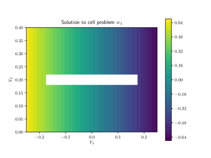
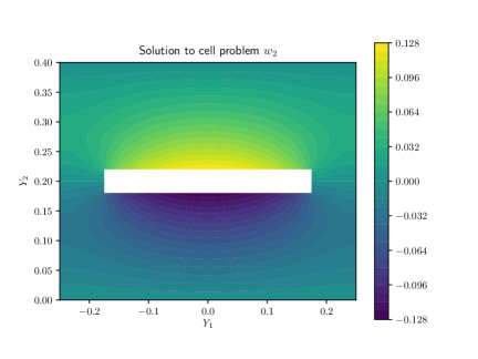
Figure 5.3: Cell functions profiles: $w_{1}$ (left) and $w_{2}$ (right).

The explicit appearance of the variable $Y_{1}$ in (3.34)–(3.37) needs to be removed by integrating the system of equations with respect to the $Y_{1}$ variable. Using the transmission conditions at $\Gamma_{\textrm{l}}$ and $\Gamma_{\textrm{r}}$, the information in $\Omega_{\textrm{m}}$ is now linked (in a well-posed way) with equation (2.8) posed in $\Omega_{\textrm{l}}$ and $\Omega_{\textrm{r}}$, respectively. The numerical approximations of the cell functions can now be used to compute the effective diffusion tensor

$$\mathbb{D}^{\star}:=\left(\begin{array}[]{cc}D_{11}^{\star}&D_{12}^{\star}\\ D_{21}^{\star}&D_{22}^{\star}\end{array}\right)=D\left(\mathbb{I}+\left(\begin{array}[]{cc}0&0\\ \frac{\partial w_{1}}{\partial Y_{2}}&\frac{\partial w_{2}}{\partial Y_{2}}\end{array}\right)\right),$$ (5.78)

and hence, FEM approximations of the upscaled diffusion-drift equation can be reached. Note that $D^{-1}\mathbb{D}^{\star}$ is the so-called membrane tortuosity tensor. Typical macroscopic concentration profiles are shown in Figure 5.4. For the chosen parameter regime, one can see that the membrane is usually permeable. Interestingly, the efficiency of the transport through the membrane reduces when increasing the strength of the drift $b$. Figure 5.4 (right) is obtained via turning the diagonal matrix $\mathbb{D}^{\star}$ into a full matrix by adding diffusion correlations. The off-diagonal entries are small $D_{12}\star=-0.05$ and $D_{21}^{\star}=+0.05$. Combined with a polynomial drift (of type $bu(1-u)$ with $b=54$) this causes some sort of anisotropic clogging.

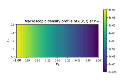
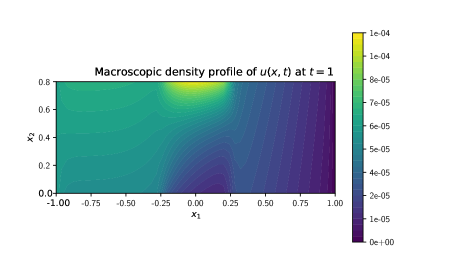
Figure 5.4: Typical macroscopic diffusion profiles. Left: A moderate permeability regime; Right: Increased barrier regime exhibiting a nearly empty membrane. Interestingly, the membrane starts to behave like a barrier only in the high drift regime (i.e. for large $b$).

Although the finite-thickness membrane scaling is rather standard (in the sense that the structure of the upscaled coefficients was foreseeable), Figure 5.5 (left) points out an outstanding opportunity: The numerical example shows that changing the aspect ratio of the rectangular obstacle can be used as tool to optimize the membrane performance (in the spirit of shape optimization). This inspired the following key question: Is such non-monotonic behavior specific to the choice of rectangles as microstructures, or is it actually generic?

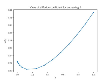
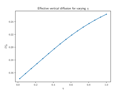
Figure 5.5: Non-monotonicity of $D_{22}^{\star}$ with respect to $\delta$, as arising in (5.76)–(5.77). Stability of $D_{22}^{\star}$ with respect to the height of the periodic cell $\eta$.

To answer this question, intensive simulations involving a large variety of shapes of microstructures need to be performed, but this is a problem by itself. For instance, the possibility of ”concentration trapping” needs to be studied by, for instance, carefully considering the effect of the curvature of the micro-boundaries on the macroscopic outflux. We will address this issue somewhere else. At this moment, relying on the stability with respect to changes in $\eta$ shown in Figure 5.5 (right), we only speculate that the answer to the question is affirmative. If this were true, then, somewhat similarly to the work done in [17], one can start thinking of optimizing filtration processes by searching for best-suitable microstructure shapes. This would be a useful tool for a number of engineering applications. What the finite membrane scaling is concerned, the optimization problem is straightforward, since it can be linked exclusively to the structure of the cell problem. For the second scaling instead, i.e. for the infinitely-thin upscaled membrane model, the optimization problem is not easily accessible. Here, any route towards optimizing filtration needs to take into account the structure of the limit two-scale model with nonlinear transmission condition; see (4.65)–(4.73).

6 Discussion

Starting from a mean-field limit of a totally asymmetric simple exclusion process (TASEP), we have investigated the problem of diffusion and non-linear drift through a composite membrane in two specific scaling regimes. We have obtained upscaled model equations for the finite-length membrane as well as for the infinitely-thin membrane. We can explicitly see how the membrane microstructure affects the resulting upscaled equations and the entries of the tensorial effective transport coefficients and our simulations show that these effects are visible at the macroscale. From the perspective of material design, we have seen that at least what concerns the penetration of CO₂ through paper, there are parameter options that can be used to optimize the membrane performance by carefully exploring the effect of the choice of the microstructure shapes on the effective transport fluxes.

To gain additional confidence in the model equations further investigations are needed. Two directions are more prominent:

(i) The upscaling needs to be made mathematically rigorous. We foresee that the two-scale convergence and boundary layer working techniques from [24] can be adapted to our scenario, provided one can handle the passage to the homogenization limit in the non-linear drift terms in both scalings. Additionally, the knowledge of the asymptotic expansions behind the singular perturbation (dimension reduction)–homogenization procedure can potentially be used to derive convergence rates for the involved limiting processes.

(ii) The stochastic particle simulations from [6] need to be extended from the one-barrier-case to the thin composite case. Then the stationary concentration profiles and the particles residence time can be compared with findings based on the finite element approximations of the upscaled model (both single and two-scale). We have chosen to include solid rectangles as microstructures precisely so that the comparison between the lattice model and the upscaled evolution equations becomes possible. Such comparison would shed light not only on transport matters through thin porous layers (like gaseous O₂ and CO₂ through paper), but would also bring understanding on the effect the knowledge of the heterogeneous environments has on the stochastic dynamics of active particles (agents).

Acknowledgments.

AM and ENMC thank Prof. Rutger van Santen (Eindhoven) for fruitful discussions that have initiated this investigation. AM acknowledges a partial financial support from NWO-MPE ”Theoretical estimates of heat losses in geothermal wells” (grant No.657.014.004). ENMC thanks FFABR 2017 financial support.

References

• [1] M. S. Alnaes, J. Blechta, J. Hake, A. Johansson, B. Kehlet, A. Logg, C. Richardson, J. Ring, M. E. Rognes, G. N. Wells, The FEniCS Project Version 1.5, Archive of Numerical Software, vol. 3, 2015.
• [2] G. Allaire, M. Briane, R. Brizzi, Y. Capdeboscq, “Two asymptotic models for arrays of underground waste containers”. Applicable Analysis 88, 10-11, 1145–1467 (2009).
• [3] B. Amaziane, L. Pankratov, V. Prytula, “Homogenization of one phase flow in a highly heterogeneous porous medium including a thin layer”. Asmptotic Analysis 70, 51–86 (2010).
• [4] E.N.M. Cirillo, G. Gonnella, A. Pelizzola, ”Folding transitions of the triangular lattice in a discrete three-dimensional space.” Phys. Rev. E 53, 3253 (1996).
• [5] E.N.M. Cirillo, O. Krehel, A. Muntean, R. van Santen, A. Sengar, “Residence time estimates for asymmetric simple exclusion dynamics on strips.” Physica A 442, 436–457 (2016).
• [6] E.N.M. Cirillo, O. Krehel, A. Muntean, R. van Santen, ”A lattice model of reduced jamming by barrier.” Physical Review E 94, 042115 (2016).
• [7] I. de Bonis, A. Muntean, ”Esistence of weak solutions to a nonlinear reaction-diffusion system with singular sources”. Electronic Journal of Differential Equations, 202 (2017).
• [8] I. de Bonis, L. M. De Cave, ”Degenerate parabolic equations with singular lower order terms”. Differential and Integral Equations 27 (9-10), 949–976 (2014).
• [9] I. de Bonis, D. Giachetti, ”Nonnegative solutions for a class of singular parabolic problems involving p-Laplacian”. Asymptotic Analysis 91 (2), 147–183 (2015).
• [10] B. Derrida, S.A. Janowsky, J.L. Lebowitz, E.R. Speer, ”Exact solution of the totally asymmetric simple exclusion process: shock profiles.” J. Stat. Phys. 73, 813–842 (1993).
• [11] A. De Masi, E. Presutti, E. Scacciatelli, ”The weakly asymmetric simple exclusion process.” Annales de l’I.H.P., section B 25, 1–38 (1989).
• [12] P. Donato, A. Piatnitski, ”On the effective interfacial resistance through rough surfaces”. Comm. Pure Appl. Analysis 9, 5, 1295–1310 (2010).
• [13] H. Ene, B. Vernescu, ”Homogenization of a singular perturbation problem”. Rev. Roumaine Math. Pures Appl. 30, 815–822 (1985).
• [14] E. R. Ijioma, A. Muntean, T. Ogawa, ”Effect of material anisotropy on the fingering instability in reverse smoldering combustion”. International Journal of Heat and Mass Transfer 81, 924–938 (2015).
• [15] M. Gahn, M. Neuss-Radu, P. Knabner, ”Derivation of an effective model for metabolic processes in living cells including substrate channeling”. Vietnam J. Math. 45, 5, 265–293 (2017).
• [16] M. Gahn, M. Neuss-Radu, P. Knabner, ”Derivation of effective transmission conditions for domains separated by a membrane for different scalings of membrane diffusivity”. DCDS Ser. S. 10, 4, 773–797 (2017).
• [17] J. G. Herterich, Q. Xu, R. W. Field, D. Vella, I. M. Griffiths, ”Optimizing the operation of a direct-flow filtration device”. J. Eng. Math. 104, 195–211 (2017).
• [18] U. Hornung, ”Homogenization and Porous Media”. vol. 6, Interdiscipinary and Applied Mathematics, Springer Verlag, 1997.
• [19] E.R. Ijioma, T. Ogawa, A. Muntean, T. Fatima, ”Homogenization and dimension reduction of filtration combustion in heterogeneous thin layers”. Networks and Heterogeneous Media 9, 4, 709–737 (2014).
• [20] C. Kipnis, C. Landim, ”Scaling Limits of Interacting Particle Systems”, Springer–Verlag, Berlin Heidelberg (1999).
• [21] G. A. Martinez-Hemosila, B. Mesic, J. E. Bronlund. ”A review of thermoplastic composites vapour permeability models: Applicability for barrier dispersion coatings”. Packag. Technol. Sc., 28, 565–578 (2015).
• [22] A. Muntean, M. Böhm, J. Kropp. ”Moving carbonation fronts in concrete: A moving-sharp-interface approach”. Chem. Eng. Sci., 66, 538–547 (2011).
• [23] D.R. Nelson, T. Piran, S. Weinberg, ”Statistical Mechanics of Membranes and Surfaces”, (World Scientific, Singapore, second edition, 2004).
• [24] M. Neuss–Radu, W. Jäger, ”Effective transmission conditions for reaction-diffusion processes in domains separated by an interface”. SIAM Journal of Mathematical Analysis 9, 4, 709–737 (2007).
• [25] A. Nyflött, L. Axrup, G. Carlson, L. Järnstrom, M. Lestelius, E. Moons, T. Wahlström, ”Influence of kaolin addition on the dynamics of oxygen mass transport in polyvinyl alcohol dispersion coatings”. Coating - Nordic Pulp & Paper Research Journal 30, 3, (2015).
• [26] C. Pozrikidis, D. M. Ford, ”Conductive transport through a mixed-matrix membrane”. J. Eng. Math. 105, 189–202 (2017).
• [27] H. Zhao, Z. Yao, ”Effective models of the Navier-Stokes flow in porous media with a thin fissure”. J. Math. Anal. Appl. 387, 542–555 (2012).
• [28] K. Sato, K. Fujimoto, M. Nakata, N. Shikazono, ”Evidence for enhanced matrix diffusion in geological environment”. Journal of the Physical Society of Japan, 82, 014901 (2013).